Statistical thresholds for Tensor PCA

Abstract.

We study the statistical limits of testing and estimation for a rank one deformation of a Gaussian random tensor. We compute the sharp thresholds for hypothesis testing and estimation by maximum likelihood and show that they are the same. Furthermore, we find that the maximum likelihood estimator achieves the maximal correlation with the planted vector among measurable estimators above the estimation threshold. In this setting, the maximum likelihood estimator exhibits a discontinuous BBP-type transition: below the critical threshold the estimator is orthogonal to the planted vector, but above the critical threshold, it achieves positive correlation which is uniformly bounded away from zero.

1. Introduction

Suppose that we are given an observation, $Y$, which is a $k$-tensor of rank $1$ in dimension $N$ subject to additive Gaussian noise. That is,

$$Y=\lambda\sqrt{N}X^{\otimes k}+W,$$ (1.1)

where $X\in\mathbb{S}^{N-1}$, the unit sphere in $\mathbb{R}^{N}$, $W$ is an i.i.d. Gaussian $k$-tensor with $W_{i_{1}\ldots i_{k}}\sim\mathcal{N}(0,1)$, and $\lambda\geq 0$ is called the signal-to-noise ratio. Throughout this paper, we assume that $X$ is drawn from an uninformative prior, namely the uniform distribution on $\mathbb{S}^{N-1}$. We study the fundamental limits of two natural statistical tasks. The first task is that of hypothesis testing: for what range of $\lambda$ is it statistically possible to distinguish the law of $W$, the null hypothesis, from the law of $Y$, the alternative? The second task is one of estimation: for what range of $\lambda$ does the maximum likelihood estimator of X, $\widehat{x}^{\rm ML}_{\lambda}(Y)$, achieve asymptotically positive inner product with $X$?

When $k=2$, this amounts to hypothesis testing and estimation for the well-known spiked matrix model. Here, maximum likelihood estimation corresponds to computing the top eigenvector of $Y$. This problem was proposed as a natural statistical model of principal component analysis [34]. It is a fundamental result of random matrix theory that there is a critical threshold below which the spectral theory of $Y$ and $W$ are asymptotically equivalent, but above which the maximum likelihood estimator achieves asymptotically positive inner product with $X$—called the correlation of the estimator with $X$—where the correlation increases continuously from $0$ to $1$ as $\lambda$ tends to infinity after $N$ [25, 6, 51, 7, 26, 17, 13]. This transition is called the BBP transition after the authors of [6] and has received a tremendous amount of attention in the random matrix theory community. Far richer information is also known, such as universality, large deviations, and fluctuation theorems. For a small sample of work in this direction, see [43, 12, 15, 14]. More recently, it has been shown that the BBP transition is also the transition for hypothesis testing [47]. See also [23, 9, 53, 8, 39, 40, 2] for analyses of the testing and estimation problem with different prior distributions.

Our goal in this paper is to understand the case $k\geq 3$, which is called the spiked tensor problem. This was introduced [54] as a natural generalization of the above to testing and estimation problems where the data has more than two indices or requires higher moments, which occurs throughout data science [42, 24, 3]. In this setting, it is known that there is an order 1 lower bound on the threshold for hypothesis testing which is asymptotically tight in $k$ [54, 52] and an order 1 upper bound on the threshold for estimation via the maximum likelihood [47, 52]. On the other hand, if one imposes a more informative, product prior distribution, i.e., $X\sim\mu_{0}^{\otimes N}$ for some $\mu_{0}\in\Pr(\mathbb{R})$, the threshold for minimal mean-square error estimation (MMSE) has been computed exactly [38, 41, 10] as has the threshold for hypothesis testing under the additional assumption that $\mu_{0}$ is compactly supported [52, 19, 20]. We note that by a standard approximation argument (see Proposition 5.8 below), the results of [41, 10] also imply a sharp threshold $\lambda_{c}$ for which the MMSE achieves non-trivial correlation for the uniform prior considered here.

The authors of [11] and [55] began a deep geometric approach to studying this problem by studying the geometry of the sub-level sets of the log-likelihood function. In [11], the authors compute the (normalized) logarithm of the expected number of local minima below a certain energy level via the Kac-Rice approach and show that there is a transition at a point $\lambda_{s}$ such that for $\lambda<\lambda_{s}$ this is negative for any strictly positive correlation, and for $\lambda>\lambda_{s}$ it has a zero with correlation bounded away from zero. The work [55] study the (normalized) logarithm of the (random) number of local minima via a novel (but non rigorous) replica theoretic approach. In particular, they predict that this problem exhibits a much more dramatic transition than the BBP transition. They argued that there are in fact two transitions for the log-likelihood, called $\lambda_{s}$ and $\lambda_{c}$. First, for $\lambda<\lambda_{s}$, all local maxima of the log-likelihood only achieve asymptotically vanishing correlation. For $\lambda_{s}<\lambda<\lambda_{c}$, there is a local maximum of the log-likelihood with non-trivial correlation but the maximum likelihood estimator still has vanishing correlation. Finally, for $\lambda_{c}<\lambda$ the maximum likelihood estimator has strictly positive correlation. In particular, if we let $m(\lambda)$, denote the limiting value of the correlation of the maximum likelihood estimator and $X$, they predict that $m(\lambda)$ has a jump discontinuity at $\lambda_{c}$. Finally, they predict that $\lambda_{c}$ should correspond to the hypothesis testing threshold. We verify several of these predictions.

We obtain here the sharp threshold for hypothesis testing and estimation by maximum likelihood and show that they are equal to $\lambda_{c}$. Furthermore, we compute the asymptotic correlation between $\widehat{x}^{\rm ML}_{\lambda}$ and $X$, $(\widehat{x}^{\rm ML}_{\lambda},X)$, where $(\cdot,\cdot)$ denotes the Euclidean inner product. We find that the maximum likelihood estimator achieves the maximal correlation among measurable estimators, and that it is discontinuous at $\lambda_{c}$. This is in contrast to the matrix setting ($k=2)$, where this transition is continuous. As a consequence of these results, the threshold $\lambda_{c}$ is also the threshold for multiple hypothesis testing: the maximum likelihood is able to distinguish between all of the hypotheses $\lambda>\lambda_{c}$. Finally, as a consequence of our arguments, we compute the maximum of the log-likelihood for fixed correlation $m$, call it $E_{\lambda}(m)$, and find that, for $\lambda_{s}<\lambda<\lambda_{c}$, $E_{\lambda}(m)$ has a local maximum at some $m_{s}>0$.

These testing and estimation problems have received a tremendous amount of attention recently as they are expected to be an extreme example of statistical problems that admit a statistical-to-algorithmic gap: the thresholds for estimation and detection are both order $1$ in $N$; on the other hand, the thresholds for efficient testing and estimation are expected to diverge polynomially in $N$, $\lambda_{\mathrm{alg}}=O(N^{\alpha})$. Indeed, this problem is known to be NP-hard for all $\lambda$ [30]. Sharp algorithmic thresholds have been shown for semi-definite and spectral relaxations of the maximum likelihood problem [32, 31, 35] as well as optimization of the likelihood itself via Langevin dynamics [4]. Upper bounds have also been obtained for message passing and power iteration [54], as well as gradient descent [4]. Our work complements these results by providing sharp statistical thresholds for maximum likelihood estimation and hypothesis testing.

Let us now discuss our main results and methods. We begin this paper by computing the sharp threshold for hypothesis testing. There have been two approaches to this in the literature to date. One is by a modified second moment method [47, 52], which yields sharp results in the limit that $k$ tends to infinity after $N$. The other approach, which we take here, is to control the fluctuations of the log-likelihood and yields sharp results for finite $k$. The key idea behind this approach is to prove a correspondence between the statistical threshold for hypothesis testing and a phase transition, called the “replica symmetry breaking” transition, in a corresponding statistical physics problem. For more on this connection see Section 2 below.

Previous approaches to making this connection precise apply to the bounded i.i.d. prior setting [38, 52, 19, 20]. There one may apply a techincal, inductive argument of Talagrand [57] related to the “cavity method” [44] to control these fluctuations. This approach uses the boundedness and product assumption on $\mu_{0}$ in an essential way, neither of which hold in our setting (though we note here the work [49] which applies for $\lambda$ sufficiently small). Our main technical contribution in this direction is a simpler, large deviations based approach which allows us to obtain the sharp threshold without using the cavity method. This argument applies with little modification to the product prior setting as well, though we do not investigate this here. For more on this see Remark 1.3.

We then turn to computing the threshold for maximum likelihood estimation. We begin by directly computing the almost sure limit of the normalized maximum likelihood, which is an immediate consequence of the results of [33, 21]. Combining this with of the results of [41] (and a standard approximation argument), we then obtain a sharp estimate for the correlation between the MLE and $X$ for $\lambda>\lambda_{c}$ and find that it matches that of the Bayes-optimal estimator, confirming a prediction from [28]. The fact that the MLE has non-trivial correlation down to the information-theoretic threshold $\lambda_{c}$ is surprising in this setting as it is not expected to be true for all prior distributions. See, e.g., [27].

1.1. Main results

Let us begin by stating our first result regarding hypothesis testing. Consider an observation $Y$ of a random tensor. Let $P_{\lambda}^{N}$ denote the law of (1.1). The null hypothesis is then $P_{0}^{N}$ and the alternative $P_{\lambda}^{N}$. Define for $t\in[0,1)$,

$$f_{\lambda}(t)=\lambda^{2}t^{k}+\log(1-t)+t$$ (1.2)

and let

$$\lambda_{c}=\sup\Big{\{}\lambda\geq 0\,\Big{|}\,\sup_{t\in[0,1)}f_{\lambda}(t)\leq 0\Big{\}}.$$ (1.3)

Our goal is to show that $P_{\lambda}^{N}$ and $P_{0}^{N}$ are mutually contiguous when $\lambda<\lambda_{c}$ and that for $\lambda>\lambda_{c}$ there is a sequence of tests $T_{N}$ which asymptotically distinguish these distributions. More precisely, we obtain the following stronger result regarding the total variation distance between these hypotheses which we state in the case $k$ even for simplicity.

Theorem 1.1.

For $k\geq 6$ even,

$$\lim_{N\to\infty}d_{TV}(P_{0}^{N},P_{\lambda}^{N})=\begin{cases}0&\text{if}\quad\lambda<\lambda_{c}\\ 1&\text{if}\quad\lambda>\lambda_{c}.\end{cases}$$

The preceding result shows us that the transition for hypothesis testing occurs at $\lambda_{c}$. Let us now turn to the corresponding results regarding maximum likelihood estimation.

It is straightforward to show that maximizing the log-likelihood is equivalent to maximizing $(Y,x^{\otimes k})$ over the sphere, $x\in\mathbb{S}^{N-1}$. The maximum likelihood estimator (MLE) $\widehat{x}^{\rm ML}_{\lambda}$ is then defined as

$$\widehat{x}^{\rm ML}_{\lambda}=\operatorname{arg\,max}_{x\in\mathbb{S}^{N-1}}(Y,x^{\otimes k}).$$ (1.4)

Our second result is that the preceding transition is also the transition for which maximum likelihood estimation yields an estimator which achieves positive correlation with $X$.

Let $q_{*}(\lambda)$ be defined by

$$q_{*}(\lambda)=\begin{cases}0&\text{if}\quad\lambda<\lambda_{c}\\ \operatorname{arg\,max}_{t\in[0,1)}f_{\lambda}(t)&\text{if}\quad\lambda>\lambda_{c}.\end{cases}$$ (1.5)

As shown in Lemma A.4, the function $f_{\lambda}$ admits a unique positive maximizer on $[0,1)$ when $\lambda>\lambda_{c}$, so that this is well-defined. Let $z_{k}$ denote the unique zero on $(0,+\infty)$ of

$$\varphi_{k}(z)=\frac{1+z}{z^{2}}\log(1+z)-\frac{1}{z}-\frac{1}{k}.$$ (1.6)

Finally, let

$${\rm GS}_{k}=\frac{\sqrt{k}}{\sqrt{1+z_{k}}}\left(1+\frac{z_{k}}{k}\right).$$ (1.7)

We then have the following.

Theorem 1.2.

Let $\lambda\geq 0$ and $k\geq 3$. The following limit holds almost surely

$$\lim_{N\to\infty}\frac{1}{\sqrt{N}}\max_{x\in\mathbb{S}^{N-1}}\big{(}x^{\otimes k},Y\big{)}\ =\ \begin{cases}{\rm GS}_{k}&\text{if}\ \ \lambda\leq\lambda_{c}\\ \displaystyle\sqrt{k}\frac{1+\lambda^{2}q_{*}(\lambda)^{k-1}}{\sqrt{1+\lambda^{2}kq_{*}(\lambda)^{k-1}}}&\text{if}\ \ \lambda>\lambda_{c}.\end{cases}$$ (1.8)

Furthermore, we have that for $\lambda\neq\lambda_{c}$

$$\lim_{N\to\infty}\Big{|}\big{(}\widehat{x}_{\lambda}^{\rm ML},X\big{)}\Big{|}=\sqrt{q_{*}(\lambda)}.$$ (1.9)

As a consequence of Corollary 5.9, the maximum likelihood estimator achieves maximal correlation. Unlike the case $k=2$, the transition in $q_{*}(\lambda)$ is not continuous. See Figure 1.1.

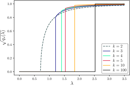
Figure 1.1. Asymptotic correlation $\lim\limits_{N\to\infty}\frac{1}{N}|\langle\widehat{x}^{\rm ML}_{\lambda},X\rangle|=\sqrt{q_{*}(\lambda)}$ as a function of the signal-to-noise ratio $\lambda$, for different values of $k$.

Let us pause for a moment to comment on the importance of the assumption that the prior is a uniform spherical prior, as opposed to, e.g., a bounded i.i.d. prior as in earlier works.

Remark 1.3.

The argument for the main hypothesis testing result Theorem 1.1 does not use in an essential way the spherical nature of the prior. The key idea is to show that a certain rate function has a locally quadratic lower bound near its zero, implying a CLT-type upper bound on fluctuations of the corresponding random variable. This estimate extends to rather broad families of problems which satisfy the “positive replicon eigenvalue” condition. See [5] for more on this condition and how it implies such bounds. However, the sphericity assumption is used in an essential way in the estimation section. The point here is that the variational problem that arises in the spherical setting has a very explicit form. As a result, one can obtain exact expressions for the transition as well as the optimizers. Using these exact expressions, we can verify that the maximum likelihood estimator is information-theoretically optimal, which plays a vital role in our argument. One can obtain a corresponding variational representation for other priors, but the variational problem is in general substantially less transparent.

Regarding the second threshold

While the regime $\lambda_{s}<\lambda<\lambda_{c}$ and the expected transition at $\lambda_{s}$ are not relevant for testing and estimation, it has a natural interpretation from the perspective of the landscape of the maximum likelihood. In [11, 55], this is explained in terms of the complexity. There is also an explanation in terms of the optimization of the maximum likelihood. We end this section with a brief discussion of this phase. Let $\lambda_{s}$ be given by

$$\lambda_{s}=\sqrt{\frac{(k-1)^{k-1}}{k(k-2)^{k-2}}}.$$ (1.10)

Consider the constrained maximum likelihood,

$$E_{\lambda}(m)=\lim_{N\to\infty}\frac{1}{N}\max_{x\in\mathbb{S}^{N-1},\,(X,x)=m}\Big{\{}\lambda N(X,x)^{k}+\sqrt{N}(W,x^{\otimes k})\Big{\}}.$$ (1.11)

This limit exists and is given by an explicit variational problem (see (5.5) below). For $\lambda>\lambda_{s}$, let ${\sqrt{q_{s}(\lambda)}}$ be the (unique) positive, strict local maximum of $f_{\lambda}$. By Lemma A.4, this is well-defined and satisfies $q_{s}(\lambda)=q_{*}(\lambda)$ for $\lambda>\lambda_{c}$. In [55], it is argued by the replica method that $E_{\lambda}(m)$ has a local maximum at $\sqrt{q_{s}(\lambda)}$ for all $\lambda>\lambda_{s}$. Establishing this rigorously is a key step in our proof of Theorem 1.2. In particular, we prove the following.

Proposition 1.4.

For $\lambda>\lambda_{s}$, the function $E_{\lambda}$ has a strict local maximum at ${\sqrt{q_{s}(\lambda)}}$. It is a global maximum of $E_{\lambda}$ if and only if $\lambda\geq\lambda_{c}$. For $\lambda\leq\lambda_{c}$ the global minimum of $E_{\lambda}$ is achieved at $m=0$.

The proof of this result immediately follows by combining Lemma 5.6 with Lemmas A.4–A.5 below.

It is easy to verify (by direct differentiation) that the map $\lambda\mapsto E_{\lambda}({\sqrt{q_{s}(\lambda)}})$ is strictly increasing on $(\lambda_{s},+\infty)$. We have also that $E_{\lambda_{c}}(\sqrt{q_{s}(\lambda_{c})})={\rm GS}_{k}$ by Lemma 5.6 and Lemma A.5, so we get that for $\lambda_{s}<\lambda<\lambda_{c}$ the strict local maximum at $\sqrt{q_{s}(\lambda)}$ has $E_{\lambda}(\sqrt{q_{s}(\lambda)})$ strictly less than the maximum likelihood. In fact, (5.5) can be solved numerically, as it can be shown that one may reduce this variational problem, in the setting we consider here, to a two-parameter family of problems in three real variables. This is discussed in Remark 5.10 below. In particular, see Figure 1.2 for an illustration of these two transitions in the case $k=4$.

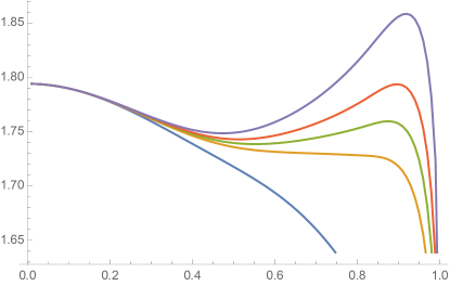
Figure 1.2. Asymptotic constrained maximum likelihood $E_{\lambda}(m)$ for $p=4$ with $\lambda=1,1.299,1.35,1.405,1.5$. Here $\lambda_{s}\approx 1.299$ and $\lambda_{c}\approx 1.405$. For $\lambda<\lambda_{s}$, the function is (numerically) seen to be monotone. A secondary maximum occurs at the transition $\lambda=\lambda_{s}$. This local maximum is bounded away from $m=0$. Finally, at the information theoretic threshold $\lambda_{c}$, the maximum likelihood is now maximized at this second point.

Let us now compare this with the complexity based approach in [11, 55]. In [11], the authors computed the expected number of local maxima of a fixed likelihood and correlation (called the annealed 0-complexity) on the exponential in $N$ scale. They showed that for $\lambda<\lambda_{s}$ this expectation scales like $O(e^{-cN})$ for correlations $q>0$, and $O(\exp(cN))$ for a suitable range of likelihoods when $q=0$, whereas for $\lambda_{s}<\lambda$, the show that at $q_{s}$, the logarithm of this quantity is $o(N)$. Furthermore, they find that once $\lambda>\lambda_{c}$, this exponent is maximized at a value of likelihood that is larger than the value for correlation $q=0$. While this argument does not show that this behavior is typical, it was argued in [55], via a novel (but non-rigorous) replica method, that the same result holds for the log-number of local maxima (called the quenched $0$-complexity) with high probability. In contrast, in this paper we bypass the analysis of critical points and instead obtain a similar picture by directly computing the almost sure limit of the constrained maximum likelihood, .

Acknolwedgements

A.J. would like to thank G. Ben Arous for encouraging the preparation of this paper. A.J. and L.M. would like to thank the organizers of the BIRS workshop “Spin Glasses and Related Topics” where part of this research was conducted. This work was conducted while A.J. was supported by NSF OISE-1604232 and P.L. was partially supported by the NSF Graduate Research Fellowship Program under grant DGE-1144152.

2. Proof of Theorem 1.1 and connection to spin glasses

In this section, we prove Theorem 1.1. In particular, we connect the phase transition for the hypothesis testing problem to a phase transition in a class of models from statistical physics, which is proved in the remaining sections.

Let us begin by explaining this connection. First note that the null hypothesis is a centered Gaussian distribution on the space of $k$-tensors in $\mathbb{R}^{N}$, whereas the alternative corresponds to one with a random mean $\lambda\sqrt{N}X^{\otimes k}$. Thus by Gaussian change of density, the likelihood ratio, $dP_{\lambda}/dP_{0}$, satisfies

$$L(Y)=\frac{dP_{\lambda}}{dP_{0}}(Y)=\int\exp\left(\lambda\sqrt{N}(Y,x^{\otimes k})-N\frac{\lambda^{2}}{2}\right)dx,$$

where $dx$ denotes the uniform measure on $\mathbb{S}^{N-1}$. Observe that the total variation distance satisfies

$$d_{TV}(P_{\lambda},P_{0})=\mathbb{E}_{P_{0}}\left((1-L(Y))\mathbbm{1}_{\{L(Y)\leq 1\}}\right)=\int_{0}^{1}P_{0}(L(Y)\leq s)ds.$$ (2.1)

We will show that this probability tends to zero almost everywhere when $\lambda<\lambda_{c}$.

Let us now make the following change of notation, motivated by statistical physics. For $x\in\mathbb{S}^{N-1}$ and ${\lambda}\geq 0$, define

$$H(x)=\sqrt{N}(W,x^{\otimes k}),\quad Z({\lambda})=\int\exp(-{\lambda}H(x))\,dx.$$ (2.2)

We view $H$ as a function on $\mathbb{S}^{N-1}$, which is called the Hamiltonian of the spherical ${k}$-spin glass model in the statistical physics literature [22]. The log-likelihood ratio then has an interpretation in terms of what is called a “free energy” in the statistical physics literature. More precisely, define the free energy at temperature ${\lambda}$ for the spherical ${k}$-spin model by

$$F_{N}({\lambda})=\frac{1}{N}\log Z_{N}({\lambda})$$ (2.3)

and observe that under the null hypothesis,

$$\frac{1}{N}\log L(Y)=F_{N}(\lambda)-\frac{\lambda^{2}}{2}.$$ (2.4)

The key conceptual step in our proof is to connect the phase transition for hypothesis testing to what is called the “replica symmetry breaking” transition in statistical physics. While it is not within the scope of this paper to provide a complete description of this transition, we note that one expects this transition to be reflected in the limiting properties of $F_{N}$: if $\lambda$ is small $F_{N}$ should fluctuate around $\lambda^{2}/2$, but for large $\lambda$ it should be much smaller than $\lambda^{2}/2$. A sharp transition is expected to occur at $\lambda_{c}$. For an in-depth discussion of replica symmetry breaking transitions see [44]. In the remainder of this section we reduce the proof of our main result to the proof that the phase transition for the fluctuations of $F_{N}$ does in fact occur at $\lambda_{c}$. We then prove this phase transition exists in the next two sections.

Let us turn to this reduction. By (2.1) and the equivalence noted above,

$$d_{TV}(P_{0},P_{\lambda})=\int_{0}^{1}P_{0}\left(F_{N}(\lambda)-\frac{\lambda^{2}}{2}<\frac{\log(x)}{N}\right)dx.$$ (2.5)

We have the following theorem of Talagrand, which we state in a weak form for the sake of exposition. Here and in the following, unless otherwise specified $\mathbb{P}$ and $\mathbb{E}$ will always denote integration with respect to the law of the Gaussian random tensor $W$.

Theorem 2.1 (Talagrand [56]).

For every ${\lambda}>0$, $\mathbb{E}F_{N}({\lambda})$ is a convergent sequence. Furthermore,

$$\lim_{N\to\infty}\mathbb{E}F_{N}\leq\frac{{\lambda}^{2}}{2},$$

with equality if and only if ${\lambda}\leq\lambda_{c}$.

With this in hand, it suffices to show the following.

Theorem 2.2.

For $k\geq 4$ even, $\epsilon>0$ and ${\lambda}<\lambda_{c}$, there is a constant $C>0$ such that for every $N\geq 1$ and $x>0$,

$$\mathbb{P}\left(\left|F_{N}({\lambda})-\frac{{\lambda}^{2}}{2}\right|>\frac{x}{N}\right)\leq C\frac{1}{x^{2}N^{{\frac{k-4}{4}}-\epsilon}}.$$

Proof.

The proof of this theorem will constitute the next two sections. Let us begin by making the following elementary observations, which will reduce the theorem to certain fluctuation theorems. To this end, observe that by Chebyshev’s inequality,

$$\mathbb{P}\left(\left|F_{N}({\lambda})-\frac{{\lambda}^{2}}{2}\right|>\eta/N\right)\leq\frac{N^{2}}{\eta^{2}}\left(\operatorname{Var}(F_{N})+\left(\mathbb{E}F_{N}-\frac{{\lambda}^{2}}{2}\right)^{2}\right).$$ (2.6)

The key point in the following will be to quantify the rate of convergence in Talagrand’s theorem when $\lambda<\lambda_{c}$. This rate of convergence will also allow us to control the variance of $F_{N}$. More precisely, in the subsequent sections we will prove the following two theorems.

Theorem 2.3.

Fix $k\geq 4$ even and ${\lambda}<\lambda_{c}$. For any $\epsilon>0$ there is a $C({\lambda},\epsilon)>0$ such that for $N\geq 1$

$$\left|\mathbb{E}F_{N}-\frac{{\lambda}^{2}}{2}\right|\leq CN^{-{k/4}+\epsilon}.$$

Theorem 2.4.

Fix $k\geq 4$ even. For ${\lambda}<\lambda_{c}$ and $\epsilon>0$, for $N\geq 1$

$$\operatorname{Var}(F_{N})\leq\frac{C({\lambda})}{N^{{k/4}+1-\epsilon}}.$$

The desired result then follows upon combining Theorem 2.3 and Theorem 2.4 with (2.6). ∎

We can now prove the main theorem.

Proof of Theorem 1.1.

Suppose first that $\lambda<\lambda_{c}$. Then by Theorem 2.2 combined with (2.5), the total variation distance vanishes for $k\geq 6$ even.

Suppose now that $\lambda>\lambda_{c}$. Note

$$\mathbb{P}(F_{N}\leq\mathbb{E}F_{N}-\epsilon)\leq\exp(-N\epsilon^{2}/2)$$

by Gaussian concentration (see, e.g., [16, Theorem 5.6]). By Jensen’s inequality $\mathbb{E}F_{N}(\lambda)\leq\lambda^{2}/2$, and by Talagrand’s theorem, we know that

$$\mathbb{E}F_{N}\to F\neq{\lambda}^{2}/2,$$

so for some $\epsilon>0$,

$$\lim_{N\to\infty}\mathbb{P}(F_{N}(\lambda)-\frac{\lambda^{2}}{2}<-\epsilon)=1.$$

The desired result then follows by using this to lower bound the right side of (2.5). ∎

3. Rate of convergence of the mean and Decay of variance.

In this section, we prove Theorem 2.3. In the following we will make frequent use of the measure

$$\pi_{{\lambda}}(dx)\propto\exp(-{\lambda}H(x))\,dx$$

where $H$ is as in (2.2) and $0<{\lambda}$. We call this the Gibbs measure, which we normalize to be a probability measure. Observe that this normalization constant is given exactly by $\log Z({\lambda})$. Here and in the remaining sections, we will let $\left\langle\cdot\right\rangle$ denote expectation with respect to the (random) measure $\pi_{{\lambda}}$. We will suppress the dependence on ${\lambda}$ whenever it is unambiguous as it will always be fixed. Throughout this section, $\lambda$ will always be fixed and less than $\lambda_{c}$. It will also be useful to define the quantity

$$F_{2,N}(u,\eta;{{\lambda}})=\frac{1}{N}\log\int\int_{\lvert\lvert(x,y)\rvert-u\rvert<\eta}\exp(-{\lambda}H(x)-{\lambda}H(y))\,dx\,dy,$$

where $(x,y)$ denotes the Euclidean inner product. Evidently this is related to the large deviations rate function for the event $(x,y)\approx u$. To simplify notation, for $X^{1},X^{2}\sim\pi_{{\lambda}}$, we let

$$R_{12}=(X^{1},X^{2}).$$

The starting point for our analysis is the estimate of the rate of convergence of $\mathbb{E}F_{N}$ to ${\lambda}^{2}/2$.

Proof of Theorem 2.3.

In the following, let

$$\psi({\lambda})=\frac{{\lambda}^{2}}{2}-\mathbb{E}F_{N}.$$

By Jensen’s inequality, $\psi({\lambda})\geq 0$.

Let us now turn to an upper bound. Recall $H$ from (2.2). Observe that $H$ is centered and has covariance

$$\mathbb{E}H(x^{1})H(x^{2})=N(x^{1},x^{2})^{k}.$$

It then follows that

$$\frac{d}{d{\lambda}}\psi({\lambda})={\lambda}-\frac{1}{N}\mathbb{E}\left\langle H\right\rangle={{\lambda}}\mathbb{E}\left\langle R_{12}^{k}\right\rangle,$$

where the first equality is by definition of the Gibbs measure and the second follows by Gaussian integration by parts for Gibbs expectations, (A.6). We now claim that

$$\frac{d}{d{\lambda}}\psi({\lambda})={{\lambda}}\mathbb{E}\left\langle R_{12}^{k}\right\rangle\leq C\psi({\lambda})+\frac{C}{N^{{k/4-k\delta/2}}}.$$ (3.1)

for some constant $C>0$ and $\delta>0$ sufficiently small. With this claim in hand, we may apply Gronwall’s inequality and the lower bound from above to obtain

$$0 \leq\psi({\lambda})\leq\left(\psi(0)+\frac{1}{N^{k/2-k\delta}}\right)\exp\left(C{\lambda}\right)=\frac{C({\lambda})}{N^{{k/2-k\delta/2}}},$$

as desired. Let us now turn to the proof of this claim.

Observe that the maps $W\mapsto F_{2,N}(u,\frac{1}{N};{\lambda})$ and $W\mapsto F_{N}({\lambda})$ are uniformly ${{\lambda}}/\sqrt{N}$-Lipschitz, so that Gaussian concentration of measure (see for instance [16], Theorem 5.6) implies that there are constants $C,c{>0}$ depending only on $\lambda$ and $k$ such that for any $\delta\in(0,1/2)$, with probability at least $1-C\exp(-cN^{2\delta}),$

$$F_{2,N}(u,\frac{1}{N};{\lambda})-\mathbb{E}F_{2,N}(u,\frac{1}{N};{\lambda})\leq\frac{1}{N^{1/2-\delta}},\qquad F_{N}({\lambda})-\mathbb{E}F_{N}({\lambda})\leq\frac{1}{N^{1/2-\delta}}.$$

Thus, on this event, call it $A(u,\delta)$,

$$\frac{1}{N}\log\pi^{\otimes 2}\left(\lvert R_{12}\rvert\in(u-\frac{1}{N},u+\frac{1}{N})\right) =F_{2,N}(u,\frac{1}{N},{\lambda})-2F_{N}({\lambda}).$$ (3.2)

$$\leq 2\left(\frac{{\lambda}^{2}}{2}-\mathbb{E}F_{N}({\lambda})\right)+\left(\mathbb{E}F_{2,N}(u,\frac{1}{N},{{\lambda}})-{\lambda}^{2}\right)+\frac{C}{N^{1/2-\delta}}.$$

As we shall show in Corollary 4.4, for every $\delta>0$ there is some $c>0$ such that for $N\geq 1$ and for all $N^{-1/2+\delta}\leq u\leq 1$;

$$\mathbb{E}F_{2,N}(u,\frac{1}{N},{{\lambda}})-{\lambda}^{2}\leq-cu^{2}.$$

Let

$$v=\frac{1}{c}\left(2\psi({\lambda})+\frac{C}{N^{1/2-\delta}}+\frac{1}{\sqrt{N}}\right).$$

Then for $u^{2}\geq v$, on $A(u,\delta)$,

$$\pi^{\otimes 2}(|R_{12}|\in(u-\frac{1}{N},u+\frac{1}{N}))\leq\exp(-\sqrt{N}).$$ (3.3)

Consequently, if we take $\{u_{i}\}_{i=1}^{L}$ to be the centers of a partition of the interval $[v,1]$ into intervals of size $2/N$ , then if we let $A(\delta)=\cap_{i}A(u_{i},\delta)$,

$$\mathbb{E}\left\langle R_{12}^{k}\right\rangle \leq\mathbb{E}\left(\left\langle R_{12}^{k}\mathbbm{1}_{R_{12}^{2}>v}\right\rangle\mathbbm{1}_{A(\delta)}\right)+\mathbb{E}\left(\left\langle R_{12}^{k}\mathbbm{1}_{R_{12}^{2}\leq v}\right\rangle\mathbbm{1}_{A(\delta)}\right)+Ne^{-cN^{{2}\delta}}.$$

$$\leq N\exp(-\sqrt{N})+v^{{k/2}}+Ne^{-cN^{{2}\delta}},$$

where we use that $L\leq N$. From this it follows, by the inequality $(x+y)^{k}\leq 2^{k-1}(x^{k}+y^{k})$, that

$$\mathbb{E}\left\langle R_{12}^{k}\right\rangle\leq C\left(\psi({\lambda})^{k}+\frac{1}{N^{{k/4-k\delta/2}}}\right)$$ (3.4)

for some $C>0$, $\delta$ small enough and $N\geq 1$. The claim (3.1) then follows since $\psi(\lambda)\leq\lambda_{c}^{2}$ for all $\lambda\leq\lambda_{c}$. For this last claim, observe that $\mathbb{E}F_{N}(\lambda)$ is convex in $\lambda$ with $\mathbb{E}F_{N}(0)=0$ and right derivative $\frac{d}{d\lambda}\mathbb{E}F_{N}(0^{+})=0$, so that $\mathbb{E}F_{N}\geq 0$. As a result, $\psi(\lambda)\leq\lambda^{2}\leq\lambda_{c}^{2}$. ∎

Notice that by the above argument, we also have the following.

Corollary 3.1.

For any $k\geq 4$ even and ${\lambda}<\lambda_{c}$ and $\eta>0$, there is a $C({\lambda},\eta)>0$ such that for $N$ sufficiently large,

$$\mathbb{E}\left\langle\lvert R_{12}\rvert^{k}\right\rangle\leq\frac{C({\lambda}{,\eta})}{N^{{k/4-k\eta/2}}}.$$

Proof.

By Theorem 2.3, we have, for $N$ large enough,

$$\psi({\lambda})\leq\frac{C({\lambda}{,\eta})}{N^{{k/4-k\eta/2}}}.$$

Combining this with (3.1) yields the desired inequality. ∎

We are now in a position to prove the variance decay.

Proof of Theorem 2.4.

By the Gaussian Poincaré inequality (see for instance [16, Theorem 3.20]),

$$\operatorname{Var}(F_{N}({\lambda})) \leq\frac{1}{N^{2}}\mathbb{E}\sum_{1\leq i_{1},\ldots,i_{k}\leq N}\left(\partial_{W_{i_{1}\ldots i_{k}}}\log Z({\lambda})\right)^{2}=\frac{{\lambda}^{2}}{N}\mathbb{E}\sum_{1\leq i_{1},\ldots,i_{k}\leq N}\left\langle x_{i_{1}}\cdots x_{i_{k}}\right\rangle^{2}=\frac{{\lambda}^{2}}{N}\mathbb{E}\left\langle R_{12}^{k}\right\rangle$$

The result then follows by combining this with Corollary 3.1. ∎

4. The Parisi functional and large deviations

The main technical tool we need is a bound on the following expected value, which is related to large deviations of $\lvert R_{12}\rvert$ from its mean:

$$\mathbb{E}\frac{1}{N}\log\pi^{\otimes 2}(\lvert R_{12}\rvert\in(u-\eta,u+\eta))=\mathbb{E}F_{2,N}(u,\eta)-2\mathbb{E}F_{N}.$$

We relate the quantities $\mathbb{E}F_{2,N}(u,\eta)$ and $\mathbb{E}F_{N}$ to explicit Parisi-type formulas. In the following, let $\xi(t)=\lambda^{2}t^{k}$ and $\theta(t)=t\xi^{\prime}(t)-\xi(t)$. For $u,\Lambda\in[0,1]$ and $m\in[1,2]$, define

$$\mathcal{P}(u,m,\Lambda) =\xi(1)+(1-m)\theta(u)-\Lambda u+\frac{1}{m}\log\frac{1+\xi^{\prime}(u)-\Lambda}{1+(1-m)\xi^{\prime}(u)-\Lambda}$$ (4.1)

$$-\frac{1}{2}\left(\log(1+\xi^{\prime}(u)+\Lambda)+\log(1+\xi^{\prime}(u)-\Lambda)\right).$$ (4.2)

Then we have the following from [56]. See also [50, 37] for alternative presentations.

Theorem 4.1.

For $k\geq 2$ even, there exists a constant $C(k)>0$ such that for every $N\geq 1$, $\eta>0$, $m\in[1,2]$, $\Lambda\in[0,1]$, and $0<u<1$, we have

$$\mathbb{E}F_{2,N}(u,\eta;\lambda) \leq\mathcal{P}(u,m,\Lambda)+\mathcal{R}$$ (4.3)

where $|\mathcal{R}|\leq C\eta+\frac{C\log N}{N}$.

Proof.

We first observe that by symmetry of $H(x)$, it suffices to prove the same estimate for

$$\tilde{F}_{2,N}(u,\eta)=\frac{1}{N}\log\pi^{\otimes 2}(R_{12}\in(u-\eta,u+\eta)).$$

We apply [50, Eq. 2.22] with the choice of parameters

$$Q^{0}=Q^{1}=Q^{2}=0,\quad Q^{3}=\left(\begin{array}[]{cc}u&u\\ u&u\end{array}\right),\quad Q^{4}=\left(\begin{array}[]{cc}1&u\\ u&1\end{array}\right),$$

$$\mathbf{m}=(0,1/2,m/2,1),\quad A_{3}=\left(\begin{array}[]{cc}1+\xi^{\prime}(u)&-\Lambda\\ -\Lambda&1+\xi^{\prime}(u)\end{array}\right),$$ (4.4)

to obtain

$$\mathbb{E}{\tilde{F}}_{2,N}(u,\eta)\leq\mathcal{P}(u,m,\Lambda)+\mathcal{R},$$

where the error term $\mathcal{R}$ in [50, Eq. 2.22] satisfies

$$\mathcal{R}={C\eta}-2\left(\frac{1}{N}\log\mathbb{P}\left(\sum_{i=1}^{N}X_{i}^{2}\geq N\right)+\frac{b-1-\log b}{2}\right),$$

where $b=(1+\xi^{\prime}(u))$, the $X_{i}$ are i.i.d. gaussian random variables with variance $1/b$, as given in [50, Eq. 2.14], and $C>0$ is universal. Using the elementary bound of Lemma A.7, it follows that $\mathcal{|}R|\leq C\left(\eta+\frac{\log N}{N}\right)$. Modifying $C$ appropriately yields the desired. ∎

Lemma 4.2.

For $k\geq 4$ even, $\lambda<\lambda_{c}$ and $\epsilon>0$, there are constants $C,c>0$ such that for every $N\geq 1$, and $c>u\geq N^{-1/2+\epsilon}$, we have

$$\mathbb{E}F_{2,N}\left(u,\frac{1}{N}{;\lambda}\right)\leq\lambda^{2}-Cu^{2}.$$

Proof.

Observe that $\mathcal{P}(u,1,\Lambda)$ is $C^{2}$ in $(u,\Lambda)$ and $(0,0)$ is a critical point with Hessian

$$\operatorname{Hess}({\mathcal{P}})(0,0)=\left(\begin{array}[]{cc}0&-1\\ -1&{1}\end{array}\right).$$

This has an eigenvector of the form $(1,x)$ for some $x>0$ with strictly negative eigenvalue $-\mu<0$. It follows that for $(u,\Lambda)=(u,ux)$ we have

$$\mathcal{P}(u,1,ux)\leq\mathcal{P}(0,1,0)-Ku^{2}=\lambda^{2}-Ku^{2}$$

for $u\leq c$ for some $K,c>0$ independent of $N$. Combining this with (4.3), we obtain

$$\mathbb{E}F_{2,N}(u,\eta{;\lambda})\leq\lambda^{2}-Ku^{2}+C\left(\eta+\frac{\log N}{N}\right).$$

If we choose $\eta=1/N$ and decrease $K$, the result follows since $u^{2}\geq N^{-1+\epsilon}>\log N/N$ for $\epsilon>0$ and $N\geq 1$. ∎

Lemma 4.3.

For $\lambda<\lambda_{c}$ and $\epsilon>0$, there are $K,C>0$ such that for every $u>\epsilon$, and $N\geq 1$

$$\mathbb{E}F_{2,N}(u,\frac{1}{N})\leq\lambda^{2}-K+C\cdot\frac{\log N}{N}.$$

Proof.

Notice that

$$\frac{d}{dm}\bigg{|}_{m=1}\mathcal{P}(s,m,0) =-(s\xi^{\prime}(s)-\xi(s))+\xi^{\prime}(s)-\log(1+\xi^{\prime}(s)){=\phi_{\lambda}(s),}$$

where $\phi_{\lambda}$ is defined by (A.1). By Lemma A.4 we have $\phi_{\lambda}(s)<0$ for all $\lambda<\lambda_{c}$ and $s\in(0,1]$.

Note that $\mathcal{P}(u,1,0)=\lambda^{2}$. Thus for every $0<u\leq 1$, $\mathcal{P}(u,m,{0})<\lambda^{2}$ for some $m>1$. Observe that $\Phi(u)=\inf_{m}\mathcal{P}(u,m,0)$ is upper-semicontinuous. Thus for any $\epsilon>0$, there exists $K(\epsilon){>0}$ such that for all $u\in[\epsilon,1]$,

$$\Phi(u)<\lambda^{2}-K(\epsilon).$$

In particular, for such $u$, it follows that

$$\mathbb{E}F_{2,N}(u,{\frac{1}{N}})\leq\lambda^{2}-K(\epsilon)+C\left(\frac{\log N}{N}\right)$$

for $u>\epsilon$, which implies the desired result. ∎

Combining these two results, we obtain the following.

Corollary 4.4.

For $\lambda<\lambda_{c}$ and $\epsilon>0$ sufficiently small, there is a $c>0$ such that for $N\geq 1$,

$$\mathbb{E}F_{2,N}(u,\frac{1}{N};\lambda)\leq\lambda^{2}-cu^{2},$$

for all $N^{-1/2+\epsilon}<u\leq 1$.

Proof.

Fix $\lambda$ and $\epsilon>0$. By Lemma 4.2, there is some $c_{1},c_{2}>0$ such that for all $N\geq 1$ and $N^{-1/2+\epsilon}<u<c_{1}$,

$$\mathbb{E}F_{2,N}(u,\eta)\leq\lambda^{2}-c_{2}u^{2}$$

Now for $c_{1}<u<1$, let $K(c_{1})$ be as in Lemma 4.3. Then $K(c_{1})u^{2}<K(c_{1})$, so that, if we take $c=\min\{c_{2},K(c_{1})\}$ the result follows. ∎

5. Estimation

In this section, we prove Theorem 1.2. We begin by providing a lower bound for the maximum likelihood for every $\lambda\geq 0$ using results on the ground state of the mixed $p$-spin model recently proved in [33, 21]. We then use the information-theoretic bound on the maximal correlation achievable by any estimator from [41] to obtain the matching upper bound. We end by proving the desired result for the correlation $(\widehat{x}^{\rm ML}_{\lambda},X)$. In the remainder of this paper, for ease of notation, we let

$$H_{\lambda}(x)=H(x)+\lambda N(x,X)^{k},$$ (5.1)

where $H(x)$ is as in (2.2).

5.1. Variational formula for the ground state of the mixed $p$-spin model

We begin by recalling the following variational formula for the ground state of the mixed $p$-spin model. Consider the Gaussian process indexed by $x\in\mathbb{S}^{N-1}$:

$$Y_{N}(x)={\sqrt{N}}\sum_{p\geq 1}a_{p}\sum_{1\leq i_{1},\dots,i_{p}\leq N}g_{i_{1},\dots,i_{p}}x_{i_{1}}\dots x_{i_{p}},$$

where $g_{i_{1},\ldots,i_{p}}$ are i.i.d. standard Gaussian random variables and $\sum_{p\geq 1}2^{p}a_{p}^{2}<\infty$. The covariance of $Y_{N}$ is given by

$$\mathbb{E}\big{[}Y_{N}(x)Y_{N}(y)\big{]}={N}\xi((x,y)),$$

where $\xi(t)=\sum_{p\geq 1}a_{p}^{{2}}t^{p}.$ Let $\mathcal{C}$ denote the subset of $C([0,1])$ of functions that are positive, non-increasing and concave. For any $h\geq 0$, we let $P_{h}:\mathcal{C}\to\mathbb{R}$ be

$$P_{h}(\phi)=\int\xi^{\prime\prime}(x)\phi(x)+\frac{1}{\phi(x)}dx+(h^{2}+\xi^{\prime}(0))\phi(0).$$

Set

$$\mathcal{G}(\xi,h)=\frac{1}{2}\min_{\phi\in\mathcal{C}}P_{h}(\phi).$$ (5.2)

Let us recall the following variational formula. For $x\in\mathbb{S}^{N-1}$, we write $x=(x_{1},\dots,x_{N})$.

Theorem 5.1 ([21, 33]).

For all $h\geq 0$,

$${\lim_{N\to\infty}\frac{1}{N}\max_{x\in\mathbb{S}^{N-1}}\Big{\{}Y_{N}(x)+h\sqrt{N}\sum_{i=1}^{N}x_{i}\Big{\}}}=\mathcal{G}(\xi,h),$$

almost surely and in $L^{1}$.

Remark 5.2.

While the results of [21, 33] are stated with $\xi^{\prime}(0)=0$, they still hold when $\xi^{\prime}(0)>0$ by replacing $\xi\mapsto\xi(t)-\xi^{\prime}(0)t$ and $h^{2}\mapsto h^{2}+\xi^{\prime}(0)$ . To see this, simply note that the Crisanti-Sommers formula still holds in this setting by the main result of [18]. The reformulation from [33, Eq. (1.0.1)] is then changed by this replacement by simply repeating the integration by parts argument from [33, Lemma 6.1.1]. From here the arguments are unchanged under the above replacement.

5.2. The lower bound

By Borell’s inequality, the constrained maximum likelihood (1.11) concentrates around its mean with sub-Gaussian tails. In particular, combining this with Borell-Cantelli we see that

$$E_{\lambda}(m)=\lim_{N\to\infty}\frac{1}{N}\mathbb{E}\Big{[}\max_{x\in\mathbb{S}^{N-1},\,(x,X)=m}\Big{\{}\lambda N(x,X)^{k}+H(x)\Big{\}}\Big{]}.$$ (5.3)

Clearly, $\varliminf\frac{1}{N}\mathbb{E}\big{[}\max_{\mathbb{S}^{N-1}}H_{\lambda}\big{]}\geq E_{\lambda}(m)$ for all $m\in[-1,1]$. Recall the definition of $\lambda_{s}$ from (1.10) and $q_{s}(\lambda)$, see, e.g., Lemma A.4. If we apply this for $\lambda>\lambda_{s}$ and $m=\sqrt{q_{s}(\lambda)}>\sqrt{1-\frac{1}{k-1}}$ (by Lemma A.4), Lemma 5.6 below will immediately yield the following lower bound.

Lemma 5.3.

For all $\lambda>\lambda_{s}$,

$$\varliminf_{N\to\infty}\mathbb{E}\Big{[}\frac{1}{N}\max_{x\in\mathbb{S}^{N-1}}H_{\lambda}(x)\Big{]}\geq\sqrt{k}\frac{1+\lambda^{2}q_{s}(\lambda)^{k-1}}{\sqrt{1+\lambda^{2}kq_{s}(\lambda)^{k-1}}}.$$ (5.4)

We now turn to the proof of Lemma 5.6. We begin by observing the following explicit representation for $E_{\lambda}$.

Lemma 5.4.

For all $m\in[-1,1]$ the limit in (1.11) exists and

$$E_{\lambda}(m)={\lambda m^{k}}+\mathcal{G}(\xi_{m},0),$$ (5.5)

where $\xi_{m}(t)=(m^{2}+(1-m^{2})t)^{k}-m^{2k}$.

Proof.

We begin by observing that by rotational invariance,

$$\frac{1}{N}\mathbb{E}\Big{[}\max_{x\in\mathbb{S}^{N-1},\,(x,X)=m}\Big{\{}\lambda N(x,X)^{k}+H(x)\Big{\}}\Big{]}=\lambda m^{k}+\frac{1}{N}\mathbb{E}\Big{[}\max_{x\in\mathbb{S}^{N-1},\,x_{1}=m}H(x)\Big{]}.$$

Let $x\in\mathbb{S}^{N-1}$ such that $x_{1}=m$. Then

$$H(x)\stackrel{{\scriptstyle(d)}}{{=}}\sqrt{N}m^{k}g_{1,\dots,1}+\sqrt{N}\sum_{j=0}^{k-1}\binom{k}{j}^{1/2}m^{j}\sum_{2\leq i_{1},\dots,i_{k-j}\leq N}g_{i_{1},\dots,i_{k-j}}x_{i_{1}}\dots x_{i_{k-j}},$$

where $\big{(}(g_{i_{1},\dots,i_{p}})_{1\leq i_{1},\dots,i_{p}\leq N}\big{)}_{p\leq k}$ are i.i.d.
standard Gaussians.

So that $\mathbb{E}\big{[}\max_{x\in\mathbb{S}^{N-1},\,x_{1}=m}H(x)\big{]}=\mathbb{E}\big{[}\max_{x\in\mathbb{S}^{N-2}}H_{m}(x)\big{]}$, where $H_{m}$ is given by:

$$H_{m}(x)=\sqrt{N}\sum_{j=0}^{k-1}\binom{k}{j}^{1/2}m^{j}(1-m^{2})^{(k-j)/2}\sum_{1\leq i_{1},\dots,i_{k-j}\leq N-1}g_{i_{1},\dots,i_{k-j}}x_{i_{1}}\dots x_{i_{k-j}}.$$

The function $H_{m}$ is a Gaussian process with covariance

$$\mathbb{E}\big{[}H_{m}(x)H_{m}(y)\big{]}=N\xi_{m}((x,y)),$$

where $\xi_{m}$ is given by

$$\xi_{m}(t)=\sum_{j=0}^{k-1}\binom{k}{j}m^{2j}(1-m^{2})^{k-j}t^{k-j}=(m^{2}+(1-m^{2})t)^{k}-m^{2k}.$$ (5.6)

We conclude using Theorem 5.1 to obtain the result. ∎

We now observe that for $m$ large enough, this formula has a particularly simple form.

Lemma 5.5.

For all $|m|\geq\sqrt{1-\frac{1}{k-1}}$ we have:

$$E_{\lambda}(m)=\lambda m^{k}+\sqrt{k(1-m^{2})}.$$ (5.7)

Proof.

In the setting of Theorem 5.1 it was also shown in [33, 21] that if $\xi^{\prime}(1)+h^{2}\geq\xi^{\prime\prime}(1)$ then $\mathcal{G}(\xi,h)=\sqrt{\xi^{\prime}(1)+h^{2}}$. Since

$$\xi_{m}^{\prime}(t) =k(1-m^{2})(m^{2}+(1-m^{2})t)^{k-1}$$

$$\xi_{m}^{\prime\prime}(t) =k(k-1)(1-m^{2})^{2}(m^{2}+(1-m^{2})t)^{k-2},$$

the condition $\xi_{m}^{\prime}(1)\geq\xi_{m}^{\prime\prime}(1)$ corresponds to $(k-1)(1-m^{2})\leq 1$, i.e. $|m|\geq\sqrt{1-\frac{1}{k-1}}$. When this holds, we get that

$$E_{\lambda}(m)=\lambda m^{k}+\mathcal{G}(\xi_{m},0)=\sqrt{\xi_{m}^{\prime}(1)}=\lambda m^{k}+\sqrt{k(1-m^{2})}$$

by (5.5). ∎

We end with the desired explicit formula for $E_{\lambda}(\sqrt{q}_{s}(\lambda))$.

Lemma 5.6.

For all $\lambda>\lambda_{s}$, $\sqrt{q_{s}(\lambda)}$ is a local maximizer of $E_{\lambda}$ and if we write $x(\lambda)=\lambda^{2}kq_{s}^{k-1}(\lambda)$,

$$E_{\lambda}\big{(}\sqrt{q_{s}(\lambda)}\big{)}=\frac{\sqrt{k}}{\sqrt{1+x(\lambda)}}\Big{(}1+\frac{x(\lambda)}{k}\Big{)}.$$

Proof.

Differentiating the expression (5.7) for $m\geq\sqrt{1-\frac{1}{k-1}}$ yields

$$E_{\lambda}^{\prime}(m) =\lambda km^{k-1}-\frac{\sqrt{k}m}{\sqrt{1-m^{2}}}=k\frac{1}{1-m^{2}}\Big{(}\lambda km^{k-1}+\frac{\sqrt{k}m}{\sqrt{1-m^{2}}}\Big{)}^{-1}\Big{(}\lambda^{2}km^{2k-2}-\lambda^{2}km^{2k}-m^{2}\Big{)}$$

so that the functions $\phi_{\lambda}$, $f_{\lambda}$ and $m^{2}\mapsto E_{\lambda}(m)$ have precisely the same monoticity on $[1-\frac{1}{k-1},1)$ (recall the expression of the derivatives $f_{\lambda}^{\prime}$ and $\phi_{\lambda}^{\prime}$ given by (A.3)). Lemma A.4 gives that $q_{s}(\lambda)$ is a local maximum of $f_{\lambda}$ and $\phi_{\lambda}$ for $\lambda>\lambda_{s}$, $\sqrt{q_{s}(\lambda)}$ is therefore a local maximum of $E_{\lambda}$.

Let us now compute $E_{\lambda}(\sqrt{q_{s}(\lambda)})$. By Lemma A.4, $q_{s}(\lambda)=\frac{x(\lambda)}{1+x(\lambda)}$. Consequently,

$$E_{\lambda}(q_{s}(\lambda)^{1/2}) =\lambda q_{s}(\lambda)^{k/2}+\sqrt{k(1-q_{s}(\lambda))}=\frac{\sqrt{k}}{\sqrt{1+x(\lambda)}}\Big{(}1+\frac{x(\lambda)}{k}\Big{)}.\qed$$

5.3. The upper bound

We prove here the upper bound.

Lemma 5.7.

For all $\lambda\geq 0$,

$$\varlimsup_{N\to\infty}\mathbb{E}\Big{[}\frac{1}{N}\max_{x\in\mathbb{S}^{N-1}}H_{\lambda}(x)\Big{]}\leq{\rm GS}_{k}+\int_{0}^{\lambda}q_{*}(t)^{k/2}\,dt.$$ (5.8)

We defer the proof of this momentarily to observe the following information-theoretic bounds which will be useful in its proof.

Proposition 5.8.

Assume that $X$ is uniformly distributed over $\mathbb{S}^{N-1}$, independently from $W$. Then for all $\lambda\in(0,+\infty)\setminus\{\lambda_{c}\}$

$$\lim_{N\to\infty}\mathbb{E}\Big{[}\Big{\|}X^{\otimes k}-\mathbb{E}\big{[}X^{\otimes k}\big{|}Y\big{]}\Big{\|}^{2}\Big{]}=1-q_{*}(\lambda)^{k}.$$

This result follows from [41, 10] by approximating the uniform measure on $\mathbb{S}^{N}$ by an i.i.d. Gaussian measure. For the completeness, we provide a proof in Appendix A.3. As a consequence of this, we have the following.

Corollary 5.9.

Assume that $X$ is uniformly distributed over $\mathbb{S}^{N-1}$, independently from $W$. Then for all measurable functions $\widehat{x}:(\mathbb{R}^{N})^{\otimes k}\to\mathbb{S}^{N-1}$ and for all $\lambda\neq\lambda_{c}$ we have

$$\varlimsup_{N\to\infty}\mathbb{E}\Big{[}\big{(}\widehat{x}(Y),X\big{)}^{k}\Big{]}\leq q_{*}(\lambda)^{k/2}.$$

Proof.

Compute

$$\mathbb{E}\Big{[}\Big{\|}X^{\otimes k}-\big{(}\sqrt{q_{*}(\lambda)}\widehat{x}(Y)\big{)}^{\otimes k}\Big{\|}^{2}\Big{]} =\mathbb{E}\big{[}\big{\|}X^{\otimes k}\big{\|}^{2}\big{]}+q_{*}(\lambda)^{k}\mathbb{E}\big{[}\big{\|}\widehat{x}(Y)^{\otimes k}\big{\|}^{2}\big{]}-2q_{*}(\lambda)^{k/2}\mathbb{E}\Big{[}\big{(}\widehat{x}(Y),X\big{)}^{k}\Big{]}$$

$$=1+q_{*}(\lambda)^{k}-2q_{*}(\lambda)^{k/2}\mathbb{E}\Big{[}\big{(}\widehat{x}(Y),X\big{)}^{k}\Big{]}.$$

Recall that the posterior mean, $\mathbb{E}(X^{\otimes k}|Y)$, uniquely achieves the minimal mean squared error over all square-integrable tensor-valued estimators, $\widehat{T}(Y)$, for $X^{\otimes k}$. The proposition follows then from Proposition 5.8 which gives

$$\varliminf_{N\to\infty}\mathbb{E}\Big{[}\Big{\|}X^{\otimes k}-\big{(}\sqrt{q_{*}(\lambda)}\widehat{x}(Y)\big{)}^{\otimes k}\Big{\|}^{2}\Big{]}\geq\varliminf_{N\to\infty}\mathbb{E}\Big{[}\Big{\|}X^{\otimes k}-\mathbb{E}\big{[}X^{\otimes k}\big{|}Y\big{]}\Big{\|}^{2}\Big{]}=1-q_{*}(\lambda)^{k}.\qed$$

With this in hand we may now prove Lemma 5.7.

Proof of Lemma 5.7.

By Proposition A.1 and an application of an envelope-type theorem (see, e.g., Proposition A.3), the map $\lambda\mapsto\frac{1}{N}\mathbb{E}\big{[}\max_{\mathbb{S}^{N-1}}H_{\lambda}(x)\big{]}$ is differentiable for $\lambda\geq 0$, with derivative

$$\frac{\partial}{\partial\lambda}\mathbb{E}\Big{[}\frac{1}{N}\max_{x\in\mathbb{S}^{N-1}}H_{\lambda}(x)\Big{]}=\mathbb{E}\Big{[}{(\widehat{x}_{\lambda}^{\rm ML},X)^{k}\Big{]}.}$$ (5.9)

By [33, 21] we know that $\frac{1}{N}\mathbb{E}[\max_{\mathbb{S}^{N-1}}H_{0}\big{]}\rightarrow{\rm GS}_{k}$. The reverse Fatou lemma gives then

$$\varlimsup_{N\to\infty}\mathbb{E}\Big{[}\frac{1}{N}\max_{x\in\mathbb{S}^{N-1}}H_{\lambda}(x)\Big{]}\leq\int_{0}^{\lambda}\varlimsup_{N\to\infty}\mathbb{E}\Big{[}\big{(}\widehat{x}_{\gamma}^{\rm ML},X\big{)}^{k}\Big{]}\,d\gamma+{\rm GS}_{k}\leq\int_{0}^{\lambda}q_{*}(\gamma)^{k/2}\,d\gamma+{\rm GS}_{k},$$

where the second inequality follows from Corollary 5.9. ∎

5.4. Proof of first part of Theorem 1.2

By an elementary but tedious calculation (see Lemma A.6) the right sides of (5.4) and (5.8) are equal for $\lambda\geq\lambda_{c}$ (recall that $q_{*}(\lambda)=q_{s}(\lambda)$ for such $\lambda$). Thus for all $\lambda>\lambda_{c}$,

$$\mathbb{E}\Big{[}\frac{1}{N}\max_{x\in\mathbb{S}^{N-1}}H_{\lambda}(x)\Big{]}\xrightarrow[N\to\infty]{}\sqrt{k}\frac{1+\lambda^{2}q_{*}(\lambda)^{k-1}}{\sqrt{1+\lambda^{2}kq_{*}(\lambda)^{k-1}}}.$$ (5.10)

We will now prove that for $\lambda\leq\lambda_{c}$, $\widebar{M}_{N}(\lambda)\xrightarrow[N\to\infty]{}{\rm GS}_{k}$, where $\widebar{M}_{N}(\lambda)$ is defined by

$$\widebar{M}_{N}(\lambda)=\mathbb{E}\left[\frac{1}{N}\max_{x\in\mathbb{S}^{N-1}}H_{\lambda}(x)\right].$$

Notice that $\widebar{M}_{N}(\lambda)$ is convex as an expectation of a maximum of linear functions. By (5.9), it follows that $\widebar{M}_{N}^{\prime}(0^{+})\geq 0$. (When $k$ is odd, we use rotational invariance to see that it is in fact zero.) Consequently, $\widebar{M}_{N}$ is non-decreasing on $[0,+\infty)$.

By [33, 21] (see Theorem 5.1), $\lim_{N\to\infty}\widebar{M}_{N}(0)={\rm GS}_{k}$. By (5.10) and Lemma A.6,

$$\lim_{\lambda\to\lambda_{c}^{+}}\lim_{N\to\infty}\widebar{M}_{N}(\lambda)={\rm GS}_{k}.$$

Consequently, we obtain that for all $\lambda\in[0,\lambda_{c}]$, $\lim_{N\to\infty}\widebar{M}_{N}(\lambda)={\rm GS}_{k}$.

The almost sure convergence of (1.8) follows then from the convergence of the expectation $\widebar{M}_{N}(\lambda)$, combined with Borell’s inequality for suprema of Gaussian processes (see for instance [16, Theorem 5.8]) and the Borel-Cantelli Lemma.∎

Remark 5.10.

By (5.5) , $E_{\lambda}$ is given by a variational problem over the space $\mathcal{C}$. We first observe that one can easily solve this variational problem numerically due to the following simple reductions. First note that if we let $\xi_{m}$ be as in (5.6), then $(1/\sqrt{\xi_{m}^{\prime\prime}})^{\prime\prime}$ is strictly positive, where the prime denotes differentiation in $t$. Thus by [33, Theorem 1.2.4], the minimizer $\phi$ must be of the form $\phi(s)=\int_{s}^{1}d\nu_{s}$ where $\nu_{s}=\theta_{1}\delta_{a}+\theta_{2}\delta_{b}$, where $a,b\in[0,1]$ and $\theta_{i}\geq 0$. Thus the variational problem (5.5) is a variational problem over 4 parameters which can be solved numerically. These observations then rigorously justify the starting point of the discussion in [55, Section 4], namely the “RS” and “1RSB” calculation in [55, Sect. 4.B] in the regime they analyize, called the “$T=0$” regime there. We refer the reader there for a more in-depth discussion, see [55, Sect. 4.C].

5.5. Proof of second part of Theorem 1.2

We now turn to the second part of Theorem 1.2, namely (1.9). Let $M_{N}(\lambda)$ denote

$$M_{N}(\lambda)=\frac{1}{N}\max_{x\in\mathbb{S}^{N-1}}H_{\lambda}(x).$$

Fix $\lambda>0$. By (1.8) and Lemma A.6

$$\lim_{N\to\infty}M_{N}(\lambda)=\ell(\lambda)=\begin{cases}{\rm GS}_{k}&\text{if}\quad\lambda\leq\lambda_{c}\\ {\rm GS}_{k}+\int_{0}^{\lambda}q_{*}(\gamma)^{k/2}\,d\gamma&\text{if}\quad\lambda>\lambda_{c}.\end{cases}$$

Let $\lambda\in(0,+\infty)\setminus\{\lambda_{c}\}$. By Proposition A.1 and the Milgrom-Segal envelope theorem (see Proposition A.3), $M_{N}$ is differentiable in $\lambda$ with derivative

$$M_{N}^{\prime}(\lambda)=\big{(}\widehat{x}^{\rm ML}_{\lambda},X\big{)}^{k},$$

almost surely. As $M_{N}$ is convex in $\lambda$ (it is a maximum of linear functions), we see that for any $0<h<\lambda$,

$$\frac{M_{N}(\lambda-h)-M_{N}(\lambda)}{h}\leq M_{N}^{\prime}(\lambda)\leq\frac{M_{N}(\lambda+h)-M_{N}(\lambda)}{h}.$$

By taking the $N\to\infty$ limit, we get that almost surely

$$\frac{\ell(\lambda-h)-\ell(\lambda)}{h}\leq\varliminf_{N\to\infty}(\widehat{x}^{\rm ML}_{\lambda},X)^{k}\leq\varlimsup_{N\to\infty}(\widehat{x}^{\rm ML}_{\lambda},X)^{k}\leq\frac{\ell(\lambda+h)-\ell(\lambda)}{h}.$$ (5.11)

Since $\ell$ is differentiable for $\lambda\neq\lambda_{c}$, we may take $h\to 0$ to obtain $\lim_{N\to\infty}(\widehat{x}^{\rm ML}_{\lambda},X)^{k}=q_{*}(\lambda)^{k/2}$ almost surely, which proves (1.9).∎

Appendix A Appendix

A.1. Uniqueness of minimizers and envelope theorems

This section gathers some basic lemmas that will be useful for the analysis.

Proposition A.1.

Recall the definition (5.1) of $H_{\lambda}$. We have the following

• If $k$ is odd, then $H_{\lambda}$ has almost surely one unique maximizer over $\mathbb{S}^{N-1}$.

• If $k$ is even, then $H_{\lambda}$ has almost surely two maximizers over $\mathbb{S}^{N-1}$, $x^{*}$ and $-x^{*}$.

Proof.

We note the following basic fact from the theory of Gaussian processes, see, e.g.  [36].

Lemma A.2.

Let $(Z(t))_{t\in T}$ be a Gaussian process indexed by a compact metric space $T$ such that $t\mapsto Z(t)$ is continuous almost surely. If the intrinsic quasi-metric, $d(s,t)^{2}=\operatorname{Var}\big{(}Z(s)-Z(t)\big{)}$, is a metric, i.e., $d(s,t)\neq 0$ for $s\neq t$, then $Z$ admits a unique maximizer on $T$ almost surely.

Observe $H_{\lambda}$ is continuous on the compact $\mathbb{S}^{N-1}$. For $x_{1},x_{2}\in\mathbb{S}^{N-1}$, we have

$$\operatorname{Var}\big{(}H_{\lambda}(x^{1})-H_{\lambda}(x^{2})\big{)}=2N\big{(}1-(x^{1},x^{2})^{k}\big{)}.$$

If $k$ is odd, then the proposition follows directly from the Lemma. If $k$ is even, we apply the Lemma on the quotient space $\mathbb{S}^{N-1}/\sim$ where $\sim$ denotes the equivalence relation defined by $x^{1}\sim x^{2}\Leftrightarrow\big{(}x^{1}=x^{2}\ \text{or}\ x^{1}=-x^{2}\big{)}$. ∎

We recall the following envelope theorem of Milgrom and Segal [45]. Let $X$ be a set of parameters and consider a function $f:X\times[0,1]\to\mathbb{R}$. Define, for $t\in[0,1]$

$$V(t) =\sup_{x\in X}f(x,t)\,,$$

$$X^{*}(t) =\big{\{}x\in X\,\big{|}\,f(x,t)=V(t)\big{\}}\,.$$

Proposition A.3 (Corollary 4 from [45] ).

Suppose that $X$ is nonempty and compact. Suppose that for all $t\in[0,1]$, $f(\cdot,t)$ is continuous. Suppose also that $f$ admits a partial derivative $f_{t}$ with respect to $t$ that is continuous in $(x,t)$ over $X\times[0,1]$. Then

• $\displaystyle V^{\prime}(t^{+})=\max_{x^{*}\in X^{*}(t)}f_{t}(x^{*},t)$ for all $t\in[0,1)$ and $\displaystyle V^{\prime}(t^{-})=\min_{x^{*}\in X^{*}(t)}f_{t}(x^{*},t)$ for all $t\in(0,1]$.

• $V$ is differentiable at $t\in(0,1)$ is and only if  $\displaystyle\Big{\{}f_{t}(x^{*},t)\,\Big{|}\,x^{*}\in X^{*}(t)\Big{\}}$ is a singleton. In that case $V^{\prime}(t)=f_{t}(x^{*},t)$ for all $x^{*}\in X^{*}(t)$.

A.2. Study of the asymptotic equations

Define, for all $q\in[0,1]$

$$\phi_{\lambda}(q)=\lambda^{2}kq^{k-1}-\log(1+\lambda^{2}kq^{k-1})-\lambda^{2}(k-1)q^{k}.$$ (A.1)

Lemma A.4.

We have for all $\lambda>0$,

$$\max_{q\in[0,1)}f_{\lambda}(q)=\max_{q\in[0,1]}\phi_{\lambda}(q)$$

Furthermore, if we let $\lambda_{s}=\sqrt{\frac{(k-1)^{k-1}}{k(k-2)^{k-2}}}$:

• For $\lambda<\lambda_{s}$, then the functions $f_{\lambda}$ and $\phi_{\lambda}$ are decreasing on $[0,1)$.

• For $\lambda>\lambda_{s}$, the functions $f_{\lambda}$ and $\phi_{\lambda}$ have a strict local minimum at $q_{u}(\lambda)$ and a strict local maximum at $q_{s}(\lambda)$ where $0<q_{u}<\frac{k-2}{k-1}<q_{s}<1$, and both functions are strictly monotone on the intervals $(0,q_{u})$, $(q_{u},q_{s})$ and $(q_{s},1)$. Moreover, $q_{s}(\lambda)$ is strictly increasing in $\lambda$ and satisfies:

  $$q_{s}(\lambda)=\frac{\lambda^{2}kq_{s}(\lambda)^{k-1}}{1+\lambda^{2}kq_{s}(\lambda)^{k-1}}\,.$$ (A.2)

Finally, for $\lambda>\lambda_{c}$, $q_{*}(\lambda)=q_{s}(\lambda)$ is the unique maximizer of $f_{\lambda}$ and $\phi_{\lambda}$ over $[0,1)$.

Proof.

We have for $q\in[0,1)$

$$\phi_{\lambda}^{\prime}(q)=\frac{k(k-1)\lambda^{2}q^{k-1}}{1+\lambda^{2}kq^{k-1}}h(q)\qquad\text{and}\qquad f_{\lambda}^{\prime}(q)=\frac{h(q)}{1-q}$$ (A.3)

where $h(q)=\lambda^{2}kq^{k-1}-\lambda^{2}kq^{k}-q$. It suffices therefore to study the variations of $f_{\lambda}$. Notice also that

$$\phi_{\lambda}(q)=f_{\lambda}(q)+h(q)-\log(1+h(q)).$$

Since $f_{\lambda}^{\prime}(q)=0$ implies $h(q)=0$, this implies that

$$\max_{q\in[0,1]}\phi_{\lambda}(q)=\max_{q\in[0,1)}f_{\lambda}(q)$$

and that these maxima are achieved at the same points. Let us now study the sign of the polynomial $h(q)$:

$$h(q)=qk\lambda^{2}\big{(}q^{k-2}-q^{k-1}-\frac{1}{k\lambda^{2}}\big{)}.$$ (A.4)

One verifies easily that the polynomial $q^{k-2}-q^{k-1}$ achives its maximum at $\frac{k-2}{k-1}$ and that the value of this maximum is $\frac{(k-2)^{k-2}}{(k-1)^{k-1}}$. We get that for $\lambda<\lambda_{s}$, $h^{\prime}(q)<0$ for all $q>0$. For $\lambda>\lambda_{s}$ we get that $h$ admits exactly 3 zeros on $\mathbb{R}$: $0<q_{u}(\lambda)<q_{s}(\lambda)<1$. Since the maximum of $h$ is achieved at $\frac{k-2}{k-1}$ we get that $q_{u}(\lambda)<\frac{k-2}{k-1}<q_{s}(\lambda)$. $q_{u}<q_{s}$ are the positive roots of $q^{k-2}-q^{k-1}=\frac{1}{k\lambda^{2}}$: $q_{u}$ is therefore strictly decreasing and $q_{s}$ is strictly increasing in $\lambda$. This proves the two points of the lemma; (A.2) simply follows from the fact that $h(q_{s}(\lambda))=0$. The last statement of Lemma A.4 is then an immediate consequence of the definition of $\lambda_{c}$. ∎

Recall that $z_{k}$ is defined as the unique zero of $\varphi_{k}(z)=\frac{1+z}{z^{2}}\log(1+z)-\frac{1}{z}-\frac{1}{k}$ on $(0,+\infty)$.

Lemma A.5.

The mapping $\lambda\mapsto q_{s}(\lambda)$ is $\mathcal{C}^{\infty}$ on $(\lambda_{s},+\infty)$. Moreover $\lambda^{2}kq_{s}(\lambda_{c})^{k-1}=z_{k}$.

Proof.

The first part follows from a straightforward application of the implicit function theorem.

We get in particular that the mapping $\lambda\mapsto q_{s}(\lambda)$ is continuous for $\lambda>\lambda_{s}$. So by definition of $\lambda_{c}$ and Lemma A.4, $\phi_{\lambda_{c}}(q_{s}(\lambda_{c}))=0$. Let us write $x=\lambda^{2}kq_{s}(\lambda_{c})^{k-1}$.

$$0=\phi_{\lambda_{c}}(q_{s}(\lambda_{c}))=x-\log(1+x)-\frac{k-1}{k}xq_{s}(\lambda_{c})=x-\log(1+x)-\frac{k-1}{k}\frac{x^{2}}{1+x}\,,$$

because $q_{s}(\lambda_{c})=\frac{x}{1+x}$ (see (A.2)). This gives that $\varphi_{k}(x)=0$ and thus $x=z_{k}$. ∎

Lemma A.6.

Let $\lambda>\lambda_{c}$ and write $x(\lambda)=\lambda^{2}kq_{s}(\lambda)^{k-1}$. Then we have

$$\frac{\sqrt{k}}{\sqrt{1+x(\lambda)}}\Big{(}1+\frac{x(\lambda)}{k}\Big{)}={\rm GS}_{k}+\int_{\lambda_{c}}^{\lambda}q_{s}(\gamma)^{k/2}d\gamma\,.$$

Proof.

Let us write $g(\lambda)=\frac{\sqrt{k}}{\sqrt{1+x(\lambda)}}\big{(}1+\frac{x(\lambda)}{k}\big{)}$. By Lemma 5.6, $\sqrt{q_{s}(\lambda)}$ is a local maximizer of $E_{\lambda}$ and thus a critical point of $E_{\lambda}$. This gives

$$g^{\prime}(\lambda)=\partial_{\lambda}\Big{[}E_{\lambda}(\sqrt{q_{s}(\lambda)})\Big{]}=\partial_{\lambda}E_{\lambda}(\sqrt{q_{s}(\lambda)})=q_{s}(\lambda)^{k/2}.$$

The lemma follows then from the fact that $x(\lambda_{c})=z_{k}$ by Lemma A.5 and the definition (1.7) of ${\rm GS}_{k}$. ∎

A.3. Proof of Proposition 5.8

For $P_{0}$ a probability distribution over $(\mathbb{R}^{N})^{\otimes k}$ with finite second moment, we define the free energy

$$F_{P_{0}}(\gamma)=\frac{1}{N}\mathbb{E}\log\int P_{0}(dx)\exp\Big{(}\sqrt{\gamma N}(x,W)+{\gamma}N(x,X_{0})-\frac{1}{2}{\gamma}N\|x\|^{2}\Big{)}$$

where $X_{0}\sim P_{0}$ and ${W}_{i_{1},\dots,i_{k}}\sim\mathcal{N}(0,1)$ are independent. Proposition A.1 from [46] states that for two probability distributions $P_{1}$, $P_{2}$ on $(\mathbb{R}^{N})^{\otimes k}$ with finite second moment, we have

$$\big{|}F_{P_{1}}(\gamma)-F_{P_{2}}(\gamma)\big{|}\leq\frac{\gamma}{2}\Big{(}\sqrt{\mathbb{E}_{P_{1}}\|X_{1}\|^{2}}+\sqrt{\mathbb{E}_{P_{2}}\|X_{2}\|^{2}}\Big{)}W_{2}(P_{1},P_{2}),$$

where $W_{2}(P_{1},P_{2})$ denotes the Wasserstein distance of order $2$ between $P_{1}$ and $P_{2}$. Let $\mu_{N}$ be the distribution of $X^{\otimes k}$ when $X\sim{\rm Unif}(\mathbb{S}^{N-1})$ and let $\nu_{N}$ be the distribution of $X^{\otimes k}$ when $X\sim{\mathcal{N}(0,\frac{1}{N}Id_{N})}$. Let us compute a bound on $W_{2}(\mu_{N},\nu_{N})$. Let $X$ be drawn uniformly over $\mathbb{S}^{N-1}$, and $G\sim{\mathcal{N}(0,Id)}$, independently from $X$. Then $(X^{\otimes k},(\|G\|X/\sqrt{N})^{\otimes k})$ is a coupling of $\mu_{N}$ and $\nu_{N}$, so that, by definition $W_{2}$,

$$W_{2}(\mu_{N},\nu_{N})^{2}\leq\mathbb{E}\big{\|}X^{\otimes k}-\big{(}X\|G\|/\sqrt{N}\big{)}^{\otimes k}\big{\|}^{2}=\mathbb{E}\Big{[}\Big{(}\Big{(}\frac{1}{N}\sum_{i=1}^{N}G_{i}^{2}\Big{)}^{k/2}-1\Big{)}^{2}\Big{]}$$

where we use that $\mathbb{E}\lvert\lvert X\rvert\rvert^{k}=1$. By the law of large numbers, it then follows that

$$\lim_{N\to\infty}\lvert F_{\mu_{N}}(\gamma)-F_{\nu_{N}}(\gamma)\rvert\to 0.$$

Recall the definition (A.1) of $\phi_{\lambda}(q)$ and define $L(\gamma)=\frac{1}{2}\max_{q\in[0,1]}\phi_{{\sqrt{\gamma}}}(q)=\frac{1}{2}\max_{q\in[0,1)}f_{{\sqrt{\gamma}}}(q)$, where the equality comes from Lemma A.4. Now, [41, Theorem 1] gives that for all $\lambda\geq 0$, $F_{\nu_{N}}(\gamma)\rightarrow L(\gamma)$ as $N\rightarrow\infty$, which implies $F_{\mu_{N}}(\gamma)\rightarrow L(\gamma)$.

The “I-MMSE Theorem” from [29] (see [46, Proposition 1.4] for a statement of this result closer to the notations used here) gives that $\gamma\mapsto F_{\mu_{N}}(\gamma)$ is convex and differentiable over $[0,+\infty)$ and

$$F_{\mu_{N}}^{\prime}(\lambda^{2})=\frac{1}{2}\left(1-\mathbb{E}\Big{[}\big{\|}X^{\otimes k}-\mathbb{E}\big{[}X^{\otimes k}\big{|}Y\big{]}\big{\|}^{2}\Big{]}\right).$$

By Griffith’s lemma for convex functions, $F_{\mu_{N}}^{\prime}$ converges to $L^{\prime}$ for each $\lambda>0$ at which $L$ is differentiable. For $\gamma<\lambda_{c}^{2}$, $L(\gamma)=0$, so $L$ is differentiable on $(0,\lambda_{c}^{2})$ with derivative equal to $0$. For $\gamma>\lambda_{c}^{2}$, we know by Lemma A.4 that $f_{{\sqrt{\gamma}}}$ admits a unique maximizer $q_{*}({\sqrt{\gamma}})$ on $[0,1]$. Proposition A.3 gives that $L$ is differentiable at $\gamma$ with derivative

$$L^{\prime}(\gamma) =\frac{1}{2}(\partial_{\gamma}f_{\sqrt{\gamma}})(q_{*}(\sqrt{\gamma}))=\frac{1}{2}q_{*}(\sqrt{\gamma})^{k}.$$

We conclude that

$$\lim_{N\to\infty}\frac{1}{2}\left(1-\mathbb{E}\Big{[}\big{\|}X^{\otimes k}-\mathbb{E}\big{[}X^{\otimes k}\big{|}Y\big{]}\big{\|}^{2}\Big{]}\right)=\lim_{N\to\infty}F_{\mu_{N}}^{\prime}(\lambda^{2})=\begin{cases}0&\text{if}\ \ \lambda<\lambda_{c}\\ \frac{1}{2}q_{*}(\lambda)^{k}&\text{if}\ \ \lambda>\lambda_{c}.\end{cases}\qed$$

A.4. Elementary lemmas

We collect here the following elementary lemmas which are used in the above.

Lemma A.7.

Let $\{X_{i}\}$ be standard normal random variables, and let $S_{N}=\frac{1}{bN}\sum_{i=1}^{N}{X^{2}_{i}}.$ There is a $C>0$ such that for $N\geq 1$ and $b>1$ (possibly varying in $N$),

$$\frac{1}{N}\log\mathbb{P}(S_{N}\geq 1)\geq-\frac{1}{2}(b-1-\log b)-\frac{2\log b}{N}-C\cdot\frac{\log N}{N}.$$ (A.5)

Proof.

If we let $K=N/2$, then

$$\mathbb{P}(S_{N}\geq 1)=\frac{1}{\Gamma(K)}\int_{bK}^{\infty}y^{K-1}e^{-y}\,dy.$$

In the integrand, we may bound $y^{K-1}\geq(bK)^{K-1}$, yielding

$$\mathbb{P}(S_{N}\geq 1)\geq\frac{(bK)^{K-1}}{\Gamma(K)}\int_{bK}^{\infty}e^{-y}\,dy=\frac{(bK)^{K-1}}{\Gamma(K)}e^{-bK}.$$

By Stirling’s approximation, it then follows that

$$\frac{1}{K}\log\mathbb{P}(S_{N}\geq 1) {\geq}-(b-1-\log b)-\frac{\log b}{K}{-}C\cdot\frac{\log K}{K},$$

for some $C>0$ from which the result follows. ∎

The following result is an elementary consequence of Gaussian integration by parts. For a proof in the discrete setting, see, e.g., [48, Lemma 1.1]. The proof in our setting then follows by an elementary approximation argument.

Lemma A.8.

Let $a(x)$ and $b(x)$ be centered Gaussian processes on $\mathbb{S}^{N-1}$ for any $N\geq 1$, with smooth covariances, continuous mutual covariance

$$C(x^{1},x^{2})=\mathbb{E}a(x^{1})b(x^{2}),$$

which is assumed to be smooth and such that $\mathbb{E}\max a(x)$ is finite. Then if we let ${\pi(dx)=\exp(b(x)){dx}/Z}$, where $Z$ is chosen so that this is a probability measure,

$$\mathbb{E}\int a(x)\,d\pi=\mathbb{E}\int\int C(x^{1},x^{1})-C(x^{1},x^{2})\,d\pi^{\otimes 2}$$ (A.6)

Proof.

By the assumption on the covariances, the processes $a(x)$ and $b(x)$ are a.s. smooth [1]. By the law of large numbers, there is a collection of points $(y^{\ell})\in\mathbb{S}^{N-1}$, such that the empirical measure

$$\mathcal{E}_{n}=\frac{1}{n}\sum_{\ell=1}^{n}\delta_{y^{\ell}}$$

converges weak-* to the uniform measure. Evidently, if we let

$$\pi_{n}=\frac{\sum_{\ell=1}^{n}\exp(b(y^{\ell}))\delta_{y^{\ell}}}{\sum_{\ell=1}^{n}\exp(b(y^{\ell}))},$$

then $\pi_{n}\to\pi$ weak-* a.s. By Gaussian integration by parts, [48, Lemma 1.1],

$$\mathbb{E}\int a(x)d\pi_{n}=\mathbb{E}\int\int C(x^{1},x^{1})-C(x^{1},x^{2})d\pi_{n}^{\otimes 2}.$$

Since, $\max a(x)$, has bounded mean. The result then follows by applying the dominated convergence theorem to each side of this equality. ∎

References

• [1] Robert J. Adler and Jonathan E. Taylor, Random fields and geometry, Springer Monographs in Mathematics, Springer, New York, 2007. MR 2319516
• [2] Ahmed El Alaoui, Florent Krzakala, and Michael I Jordan, Finite size corrections and likelihood ratio fluctuations in the spiked wigner model, arXiv preprint arXiv:1710.02903 (2017).
• [3] Animashree Anandkumar, Rong Ge, Daniel Hsu, Sham M Kakade, and Matus Telgarsky, Tensor decompositions for learning latent variable models, The Journal of Machine Learning Research 15 (2014), no. 1, 2773–2832.
• [4] Gerard Ben Arous, Reza Gheissari, and Aukosh Jagannath, Algorithmic thresholds for tensor pca, arXiv preprint arXiv:1808.00921 (2018).
• [5] Gérard Ben Arous and Aukosh Jagannath, Spectral gap estimates in mean field spin glasses, Communications in Mathematical Physics 361 (2018), no. 1, 1–52.
• [6] Jinho Baik, Gérard Ben Arous, and Sandrine Péché, Phase transition of the largest eigenvalue for nonnull complex sample covariance matrices, Annals of Probability (2005), 1643–1697.
• [7] Jinho Baik and Jack W Silverstein, Eigenvalues of large sample covariance matrices of spiked population models, Journal of Multivariate Analysis 97 (2006), no. 6, 1382–1408.
• [8] Jess Banks, Cristopher Moore, Roman Vershynin, Nicolas Verzelen, and Jiaming Xu, Information-theoretic bounds and phase transitions in clustering, sparse pca, and submatrix localization, Information Theory (ISIT), 2017 IEEE International Symposium on, IEEE, 2017, pp. 1137–1141.
• [9] Jean Barbier, Mohamad Dia, Nicolas Macris, Florent Krzakala, Thibault Lesieur, and Lenka Zdeborová, Mutual information for symmetric rank-one matrix estimation: A proof of the replica formula, Advances in Neural Information Processing Systems, 2016, pp. 424–432.
• [10] Jean Barbier and Nicolas Macris, The stochastic interpolation method: A simple scheme to prove replica formulas in bayesian inference, arXiv preprint arXiv:1705.02780 (2017).
• [11] Gerard Ben Arous, Song Mei, Andrea Montanari, and Mihai Nica, The landscape of the spiked tensor model, arXiv preprint arXiv:1711.05424 (2017).
• [12] F. Benaych-Georges, A. Guionnet, and M. Maida, Large deviations of the extreme eigenvalues of random deformations of matrices, Probability Theory and Related Fields 154 (2012), no. 3, 703–751.
• [13] Florent Benaych-Georges and Raj Rao Nadakuditi, The eigenvalues and eigenvectors of finite, low rank perturbations of large random matrices, Advances in Mathematics 227 (2011), no. 1, 494–521.
• [14] Alex Bloemendal, Antti Knowles, Horng-Tzer Yau, and Jun Yin, On the principal components of sample covariance matrices, Probability theory and related fields 164 (2016), no. 1-2, 459–552.
• [15] Alex Bloemendal and Bálint Virág, Limits of spiked random matrices i, Probability Theory and Related Fields 156 (2013), no. 3-4, 795–825.
• [16] Stéphane Boucheron, Gábor Lugosi, and Pascal Massart, Concentration inequalities: A nonasymptotic theory of independence, Oxford university press, 2013.
• [17] Mireille Capitaine, Catherine Donati-Martin, and Delphine Féral, The largest eigenvalues of finite rank deformation of large wigner matrices: convergence and nonuniversality of the fluctuations, The Annals of Probability (2009), 1–47.
• [18] Wei-Kuo Chen, The Aizenman-Sims-Starr scheme and Parisi formula for mixed $p$-spin spherical models, Electron. J. Probab. 18 (2013), no. 94, 14. MR 3126577
• [19] by same author, Phase transition in the spiked random tensor with rademacher prior, arXiv preprint arXiv:1712.01777 (2017).
• [20] Wei-Kuo Chen, Madeline Handschy, and Gilad Lerman, Phase transition in random tensors with multiple spikes, arXiv preprint arXiv:1809.06790 (2018).
• [21] Wei-Kuo Chen and Arnab Sen, Parisi formula, disorder chaos and fluctuation for the ground state energy in the spherical mixed p-spin models, Communications in Mathematical Physics 350 (2017), no. 1, 129–173.
• [22] Andrea Crisanti and H-J Sommers, The sphericalp-spin interaction spin glass model: the statics, Zeitschrift für Physik B Condensed Matter 87 (1992), no. 3, 341–354.
• [23] Yash Deshpande, Emmanuel Abbe, and Andrea Montanari, Asymptotic mutual information for the balanced binary stochastic block model, Information and Inference: A Journal of the IMA 6 (2016), no. 2, 125–170.
• [24] Olivier Duchenne, Francis Bach, In-So Kweon, and Jean Ponce, A tensor-based algorithm for high-order graph matching, IEEE transactions on pattern analysis and machine intelligence 33 (2011), no. 12, 2383–2395.
• [25] SF Edwards and Raymund C Jones, The eigenvalue spectrum of a large symmetric random matrix, Journal of Physics A: Mathematical and General 9 (1976), no. 10, 1595.
• [26] Delphine Féral and Sandrine Péché, The largest eigenvalue of rank one deformation of large wigner matrices, Communications in mathematical physics 272 (2007), no. 1, 185–228.
• [27] Peter Gillin, Hidetoshi Nishimori, and David Sherrington, Multispin ising spin glasses with ferromagnetic interactions, Journal of Physics A: Mathematical and General 34 (2001), no. 14, 2949.
• [28] Peter Gillin and David Sherrington, $p>2$ spin glasses with first-order ferromagnetic transitions, Journal of Physics A: Mathematical and General 33 (2000), no. 16, 3081.
• [29] Dongning Guo, Shlomo Shamai, and Sergio Verdú, Mutual information and minimum mean-square error in gaussian channels, IEEE Transactions on Information Theory 51 (2005), no. 4, 1261–1282.
• [30] Christopher J. Hillar and Lek-Heng Lim, Most tensor problems are np-hard, J. ACM 60 (2013), no. 6, 45:1–45:39.
• [31] Samuel B Hopkins, Tselil Schramm, Jonathan Shi, and David Steurer, Fast spectral algorithms from sum-of-squares proofs: tensor decomposition and planted sparse vectors, Proceedings of the forty-eighth annual ACM symposium on Theory of Computing, ACM, 2016, pp. 178–191.
• [32] Samuel B Hopkins, Jonathan Shi, and David Steurer, Tensor principal component analysis via sum-of-square proofs, Conference on Learning Theory, 2015, pp. 956–1006.
• [33] Aukosh Jagannath and Ian Tobasco, Low temperature asymptotics of spherical mean field spin glasses, Communications in Mathematical Physics 352 (2017), no. 3, 979–1017.
• [34] Iain M Johnstone, On the distribution of the largest eigenvalue in principal components analysis, Annals of statistics (2001), 295–327.
• [35] Chiheon Kim, Afonso S Bandeira, and Michel X Goemans, Community detection in hypergraphs, spiked tensor models, and sum-of-squares, Sampling Theory and Applications (SampTA), 2017 International Conference on, IEEE, 2017, pp. 124–128.
• [36] Jeankyung Kim, David Pollard, et al., Cube root asymptotics, The Annals of Statistics 18 (1990), no. 1, 191–219.
• [37] Justin Ko, Free energy of multiple systems of spherical spin glasses with constrained overlaps, arXiv preprint arXiv:1806.09772 (2018).
• [38] Satish Babu Korada and Nicolas Macris, Exact solution of the gauge symmetric p-spin glass model on a complete graph, Journal of Statistical Physics 136 (2009), no. 2, 205–230.
• [39] Marc Lelarge and Léo Miolane, Fundamental limits of symmetric low-rank matrix estimation, Probability Theory and Related Fields (2018).
• [40] Thibault Lesieur, Florent Krzakala, and Lenka Zdeborová, Constrained low-rank matrix estimation: phase transitions, approximate message passing and applications, Journal of Statistical Mechanics: Theory and Experiment 2017 (2017), no. 7, 073403.
• [41] Thibault Lesieur, Léo Miolane, Marc Lelarge, Florent Krzakala, and Lenka Zdeborová, Statistical and computational phase transitions in spiked tensor estimation, 2017 IEEE International Symposium on Information Theory (ISIT) (2017), 511–515.
• [42] Nan Li and Baoxin Li, Tensor completion for on-board compression of hyperspectral images, Image Processing (ICIP), 2010 17th IEEE International Conference on, IEEE, 2010, pp. 517–520.
• [43] Mylène Maida, Large deviations for the largest eigenvalue of rank one deformations of gaussian ensembles, Electronic Journal of Probability 12 (2007), 1131–1150.
• [44] Marc Mézard, Giorgio Parisi, and Miguel Virasoro, Spin glass theory and beyond: An introduction to the replica method and its applications, vol. 9, World Scientific Publishing Co Inc, 1987.
• [45] Paul Milgrom and Ilya Segal, Envelope theorems for arbitrary choice sets, Econometrica 70 (2002), no. 2, 583–601.
• [46] Léo Miolane, Phase transitions in spiked matrix estimation: information-theoretic analysis, arXiv preprint arXiv:1806.04343 (2018).
• [47] Andrea Montanari, Daniel Reichman, and Ofer Zeitouni, On the limitation of spectral methods: From the gaussian hidden clique problem to rank-one perturbations of gaussian tensors, Advances in Neural Information Processing Systems, 2015, pp. 217–225.
• [48] Dmitry Panchenko, The sherrington-kirkpatrick model, Springer, 2013.
• [49] Dmitry Panchenko et al., Cavity method in the spherical sk model, Ann. Inst. Henri Poincaré Probab. Stat 45 (2009), no. 4, 1020–1047.
• [50] Dmitry Panchenko and Michel Talagrand, On the overlap in the multiple spherical sk models, Ann. Probab. 35 (2007), no. 6, 2321–2355.
• [51] Sandrine Péché, The largest eigenvalue of small rank perturbations of hermitian random matrices, Probability Theory and Related Fields 134 (2006), no. 1, 127–173.
• [52] Amelia Perry, Alexander S Wein, and Afonso S Bandeira, Statistical limits of spiked tensor models, arXiv preprint arXiv:1612.07728 (2016).
• [53] Amelia Perry, Alexander S Wein, Afonso S Bandeira, and Ankur Moitra, Optimality and sub-optimality of pca for spiked random matrices and synchronization, arXiv preprint arXiv:1609.05573 (2016).
• [54] Emile Richard and Andrea Montanari, A statistical model for tensor pca, Advances in Neural Information Processing Systems, 2014, pp. 2897–2905.
• [55] Valentina Ros, Gérard Ben Arous, Giulio Biroli, and Chiara Cammarota, Complex energy landscapes in spiked-tensor and simple glassy models: ruggedness, arrangements of local minima and phase transitions, arXiv preprint (2018), https://arxiv.org/abs/1804.02686.
• [56] Michel Talagrand, Free energy of the spherical mean field model, Probab. Theory Related Fields 134 (2006), no. 3, 339–382. MR 2226885 (2007i:82034)
• [57] by same author, Mean field models for spin glasses: Volume i: Basic examples, vol. 54, Springer Science & Business Media, 2010.