Wannier-Orbital theory and ARPES for the quasi-1D conductor LiMo₆O₁₇.
Part I: Six-band $t_{2g}$ Hamiltonian.

Abstract

In this and the two following papers, we present the results of a combined study by density-functional (LDA) band theory and angle-resolved photoemission spectroscopy (ARPES) of lithium purple bronze, Li_1xMo₆O₁₇. This material is particularly notable for its unusually robust quasi-one-dimensional (quasi-1D) behavior. The band structure, in a large energy window around the Fermi energy, is basically 2D and formed by three Mo $t_{2g}$-like extended Wannier orbitals (WOs), each one giving rise to a 1D band running at a 120^∘ angle to the two others. A structural ”dimerization” from $\mathbf{c}/2$ to $\mathbf{c}$ gaps the $xz$ and $yz$ bands while leaving the $xy$ bands metallic in the gap but resonantly coupled to the gap edges and, hence, to the two other directions. The resulting complex shape of the quasi-1D Fermi surface (FS), verified by our ARPES, thus depends strongly on the Fermi energy position in the gap, implying a great sensitivity to Li stoichiometry of properties dependent on the FS, such as FS nesting or superconductivity. The theory is verified in detail by the recognition and application of an ARPES selection rule that enables, for the first time, the separation in ARPES spectra of the two barely split $xy$ bands and the observation of their complex split FS. The strong resonances prevent either a two-band tight-binding (TB) model or a related real-space ladder picture from giving a valid description of the low-energy electronic structure. Down to a temperature of 6 K we find no evidence for a theoretically expected downward renormalization of perpendicular single particle hopping due to LL fluctuations in the quasi-1D chains. This paper I introduces the material, motivates our study, summarizes the Nth-order muffin-tin orbital (NMTO) method that we use, analyzes the crystal structure and the basic electronic structure, and presents our NMTO calculation of the $t_{2g}$ low-energy WOs and the resulting tight-binding (TB) Hamiltonian for the six lowest energy bands, only the four lowest being occupied. Thus this paper sets the theoretical framework and nomenclature for the following two papers.

Abstract

This is the second paper of a series of three papers presenting a combined study by band theory and angle-resolved photoemission spectroscopy (ARPES) of lithium purple bronze. The $t_{2g}$ Wannier Orbitals (WOs) and resulting six-band tight-binding (TB) Hamiltonian found in paper I are here used to develop a theory of the ARPES intensity variations, including a selection rule whose validity relies on the smallness of and the cancellation between the displacement- and inversion-dimerizations of the zig-zag chains (ribbons) in regions of the final-state wavevector, $\mathbf{\kappa}$. We then present the ARPES results for the band structure of the four occupied $t_{2g}$-bands (gapped $xz$, $yz$, and split metallic $xy$). A detailed comparison to the theory validates the selection rule. We present the Fermi surface (FS) as seen directly in the raw ARPES data, both parallel and perpendicular (using photon-energy dependence) to the sample surface, and show that the selection rule can enable separation of the barely split and highly quasi-one-dimensional $xy$-bands. We adjust the energy of the $xy$ WO energy by 0.1 eV ($\approx\frac{1}{4}$ of the gap) with respect to that of the gapped $xz$ and $yz$ WOs and, in a second step, fine-tune merely 7 out of the more than 40 TB parameters to achieve an excellent fit to the ARPES bands lying more than 0.15 eV below the Fermi level. So doing then also gives nearly perfect agreement closer to the Fermi level.

Abstract

This is the third paper of a series of three papers presenting a combined study by band theory and angle-resolved photoemission spectroscopy (ARPES) of lithium purple bronze. The first paper laid the foundation for the theory, and the second paper discussed a general comparison between theory and experiment, including deriving an ARPES selection rule. The present paper III focuses in detail on the two metallic, quasi-1D $xy$-like bands left in the 0.4 eV dimerization gap between the $xz$ and $yz$ valence and conduction (V&C) bands. The hybridizations with the latter change the perpendicular dispersions of –and splitting between– the resulting $\widetilde{xy}$ bands. The edges of the $\genfrac{}{}{0.0pt}{}{\mathrm{V}}{\mathrm{C}}$ bands, in particular, push resonance peaks $\genfrac{}{}{0.0pt}{}{\mathrm{up}}{\mathrm{down}}$ in the $\widetilde{xy}$ bands which are now described by a two-band Hamiltonian (121) whose two first terms consist of the pure $xy$-block of the six-band TB Hamiltonian, I Eq. (56), and whose 4 following terms describe the resonant coupling to (i.e., indirect hopping via) the V&C bands. The two-band Hamiltonian extends the selection rule derived in the previous paper to the hybridized $\widetilde{xy}$ bands, which enables, for the first time, extracting the split quasi-1D Fermi surface (FS) from the raw ARPES data. The complex shape of the FS, verified in detail by our ARPES, depends strongly on the Fermi energy position in the gap, implying a great sensitivity to Li stoichiometry of properties dependent on the FS, such as FS nesting or superconductivity. The strong resonances prevent either a two-band TB model or a related real-space ladder picture from giving a valid description of the low-energy electronic structure. Down to a temperature of 6 K, we find no evidence for a theoretically expected downward renormalization of perpendicular single-particle hopping due to LL fluctuations in the quasi-1D chains.

I Introduction

The present paper (I) and its two companion papers (II and III) are devoted to a detailed study of the band structure of the lithium purple bronze (LiPB) LiMo₆O₁₇, combining angle-resolved photoemission spectroscopy (ARPES) and Wannier function band theory using the Nth-order muffin-tin orbital method (NMTO). Since its discovery [1] and structure determination [2] LiPB has been heavily studied as a quasi-1D material [4, 5, 6, 7, 8, 9, 10, 11]. Thus, it is notable as an unusually good and interesting example of the non-Fermi liquid (non-FL) properties exhibited by one-dimensional (1D) interacting electron systems, such as in the exactly solvable Tomonaga-Luttinger (TL) model [12, 13] or in the more generalized notion of the Luttinger Liquid (LL) [14]. A highly non-intuitive example of such non-FL properties is that the energy ($E$) dependence of the momentum ($\kappa$) integrated single-particle spectral function, which would give simply the one-electron density of states in a non-interacting system, goes to zero upon approaching the Fermi-energy ($E_{F}$) as a power law $\left(E_{F}-E\right)^{\alpha}$, with $\alpha$ interpreted as the anomalous exponent of the TL model.

FIG. 1 reproduces angle-integrated data from a previous photoemission study [3], showing this unusual property for LiPB for the spectral function below $E_{F}$, as probed by ARPES. The spectra for $\kappa$-integration along the quasi-1D direction, for temperatures $T$=4 K and 30 K and resolution 5 meV, are well described by a power law with $\alpha$=0.7 over at least 40 meV, compared to the Fermi edge of a $T$=4 K gold reference spectrum. Also, scanning tunneling spectroscopy [15], which probes the spectral function on both sides of $E_{F}$, shows the power law ”V-shape” down to 4 K . It is then equally non-intuitive in the TL model that, nonetheless, the underlying band-structure Fermi momentum $k_{F}$ and thus, the Fermi surface (FS) remains well-defined [16]. Paper III presents a detailed determination of the FS for LiPB.

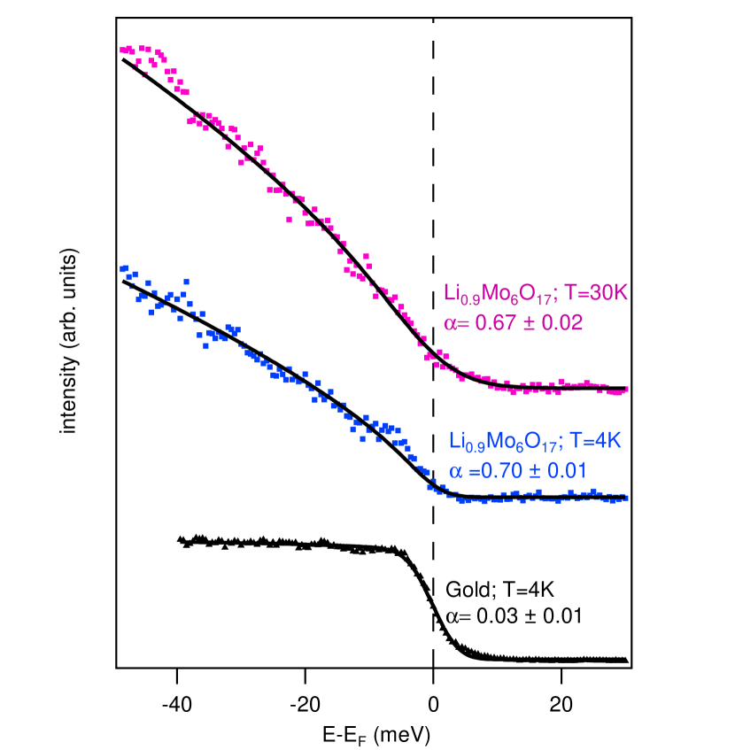
Figure 1: Angle integrated photoemission spectra of lithium purple bronze for $T$=4 and 30 K taken with a resolution of 5 meV with photon energy $h\nu$=8.4  eV [3]. For reference, a gold spectrum with the same settings is also shown. All the spectra are generally well fitted by the TL-model lineshape, showing for LiMo₆O₁₇ a value of $\alpha\approx 0.7$. In Ref. 3, it was deemed ambiguous whether a very noisy feature around 5 meV in the fit residuals is intrinsic or arises from some systematic experimental error. The gold spectrum fits well with $\alpha$ essentially zero, corresponding mathematically to a Fermi edge.

The band structure and, in particular, the magnitude(s) of the transverse hoppings ($t_{\perp}$) between its 1D chains, and the resulting FS, are especially interesting and important for LiPB. The general theoretical expectation [14] is that, for $T$ decreasing below a scale set by $t_{\perp}$, LL behavior is unstable against dimensional crossover from 1D to some sort of 3D Fermi-liquid (FL) behavior, typically by a phase transition to some 3D ordered state like a charge or spin density wave (CDW or SDW). Band calculations to date suggest values of $t_{\perp}$=20 meV (232 K) and yet the data of FIG. 1 indicate that its non-FL 1D properties likely last until the material goes superconducting (SC) at $T_{SC}$=1.9 K. Indeed other properties of LiPB, albeit novel and interesting, exhibit no clear evidence for dimensional crossover above $T_{SC}$ [3]. However, theory [14] also suggests that LL fluctuations on the chains can strongly suppress the single-particle hopping and consequently the crossover $T$. For example, in the case of one chain per primitive cell and hopping only to the nearest chain, the suppression of $t_{\perp}$ is by the factor $(t_{\perp}/t)^{\alpha/(1-\alpha)}$, where $t\gg t_{\perp}$ is the hopping along the chains. For a typical band-theory value of $\left|t\right|$=0.8 eV [17] and the value of $\alpha$=0.7 cited above, one obtains $t_{\mathrm{eff}\,\perp}$ = 4$\,\mu$eV or 0.04 K, even smaller than $T_{SC}$.. Such a small value might thus account for the exceptional stability of 1D physics in this material, and should be manifest in the low-$T$ single-particle electronic structure. However, up to now, the transverse hopping and resulting FS have never been measured experimentally or characterized theoretically as fully as is needed and possible.

There is additional motivation for our study. As described in detail further below, LiPB is complex in having two approximately 1D bands associated with there being two equivalent chains (and two formula units) per primitive cell, each half filled for stoichiometric LiMo₆O₁₇. Thus most LiPB theories to date [17, 4, 5, 6, 7, 9, 10, 11] have modeled the quasi-1D electrons as a lattice of pairs of chains regarded as ladders, with simple tight-binding (TB) $t_{\perp}$ and $t_{\perp}^{\prime}$ parameters for nearest neighbor intra- and inter-ladder hopping, respectively. So it is of great interest to check the validity of the ladder picture, which involves the relative magnitudes of the perpendicular hoppings within and between primitive cells. These hoppings determine the perpendicular dispersion and splitting of the two bands forming the FS. Of particular interest is the normal state FS giving rise to SC. The FS also gives the clearest experimental access to the details of the transverse hoppings.

Another motivation is to demonstrate the use of the NMTO method for creating chemically meaningful Wannier functions –in the present case Wannier orbitals (WOs) centered on Mo1, the only octahedrally fully coordinated molybdenum (Sect. III.1)– and their TB Hamiltonian, and to establish them as important tools for predicting and interpreting the ARPES data. As summarized in more detail below, like the study in Ref. 19, our theory uses the local density-functional approximation (DFT-LDA) to derive a set of localized Wannier functions, which, however, in our case, is complete in the sense that it contains all three Mo1 4$d\,t_{2g}$-like orbitals per formula unit, and thereby spans the occupied as well as the lowest empty bands. The two quasi-1D metallic bands are $xy$-like and situated in a 0.4 eV gap between valence bands formed by the $xz$ and $yz$ WOs, bonding between the ladder rungs, and conduction bands formed by the same WOs, but antibonding between rungs. After integrating out the $xz$ and $yz$ degrees of freedom (in Paper III), our theory leads to the conclusions, that the effective transverse couplings between the two quasi-1D bands cannot be described by a simple TB model, and also that they have very long range, making ladders ill-defined. In this respect all previous TB ladder models are very unrealistic.

The theory also leads to a selection rule (in Paper II) that enables the two barely split quasi-1D bands to be separated in the ARPES spectra near $E_{F}$ for the first time. The split and warped FS obtained thereby in ARPES at 6 K is in excellent agreement with the predicted FS, giving a detailed confirmation of the theory (Paper III). This means that the predicted LL renormalization of the perpendicular hoppings with decreased temperature does not occur, and so cannot be the origin of the robustness of the LiPB 1D behavior. We can also infer that the LDA FS is the normal state FS relevant for theories [6, 7, 9, 20, 21] of the SC. We note that the occurrence of SC is sample dependent [22], and, in this context, that the details of the theoretical FS shape are extremely sensitive to the position of $E_{F}$, which is controlled by the Li-content (or the content of oxygen vacancies). For our samples, the $E_{F}$ position indicates that they are very nearly stoichiometric, which is the circumstance found in theory to give the most 1D FS. Although we have not explicitly verified SC for our samples, these findings are consistent with the hypothesis that SC has a 1D origin and that the absence of SC in some samples may be linked to sample stoichiometry through the sensitivity of the FS. Finally, although $T$ dependence was not a particular focus of the experiments, we find the same FS at 30K, implying that a mysterious resistivity upturn below $T_{M}\approx$ 25K is not likely to be associated with a gross change in electronic structure [3].

Before proceeding we emphasize that our purpose is not merely to present the numerical results of yet another DFT-LDA calculation for LiPB. Rather, DFT-LDA is a tool to implement the overall program described in the three papers. We use it to obtain chemically meaningful NMTO WOs, which, in turn, we use to gain new insight into how the numerical results come about. The central theory result is a portable six-band analytic TB Hamiltonian to describe the low-energy band structure. The agreement of its eigenvalues with the ARPES band structure is already generally good using LDA parameter values and can be made excellent by some additional adjustments, showing that its functional forms are faithful to the physics. Further, along with its underlying WOs, it can be used to understand the complex ARPES intensity variations in unprecedented detail, in particular the selection rule already mentioned. Ultimately the combination of new theory insight and ARPES experiment yields new knowledge of the details of the Fermi surface and the magnitude and range of the perpendicular hopping for the two metallic bands.

In the remainder of this introductory section, we give a more detailed overview of the theory relative to previous work, and describe the division of content between the three papers.

The basic band structure in the vicinity of $E_{F}$ has been known for many years from pioneering TB calculations based on the semi-empirical extended-Hückel method [24]. There are two approximately 1D-bands dispersing across $E_{F}$, associated with there being two equivalent chains of Mo atoms having a zigzag arrangement (zig-Mo1-zag-Mo4-zig), and two formula units per primitive cell. The two bands have Mo 4$d_{xy}$ character and for stoichiometric LiMo₆O₁₇ they are half-filled. There are also two filled bands not far below $E_{F}$.

Quantitatively correct band structures require charge-self-consistent DFT calculations, not a small task for a transition-metal oxide with 48 atoms per cell, so it took nearly twenty years for the first self-consistent DFT (LDA) band structure to appear [25] and another six for the second [26]. Both calculations were performed with the linear muffin-tin orbital method (LMTO) in the atomic-spheres approximation. Such LDA-LMTO band structures provided guidance for the TB band-structure parameters used in early many-body models [4, 17]. Higher-resolution low-temperature ARPES data and more accurate NMTO calculations show agreement even on the details [27] of the filled bands.

An alternative TB model [19] has been derived by first using the highly accurate full-potential linear augmented-plane-wave (LAPW) method to perform a charge self-consistent DFT (LDA) calculation of the band structure over a wide energy range, and then projecting from it a set of four so-called maximally localized Wannier functions, which describe the two quasi-1D bands and the two valence bands. The Wannier functions of this model are therefore not atomic, but essentially the bonding linear combination of those on Mo1 and Mo4, and the integral for hopping between these $xy$-bond orbitals is only about half the one for hopping between the atomic orbitals considered in the TB models previously used [4, 17]. The study of Nuss and Aichhorn [19] also provides a simplified two-band TB Hamiltonian by folding the two occupied $xz$ and $yz$ bands down into the two $xy$ bands, thereby becoming $\widetilde{xy}$ bands, and fitting their hybridization such as to modify the $t_{\perp}$ parameters. The result is said to be in good agreement with those discussed in Ref. 17.

For the theory of the present paper and its two companion papers, early results of which were given in Ref. [27], we need and provide an improved 3D visualization of the crystal structure, with an associated wording (Sect. III of the present paper): ribbons containing Mo1, Mo2, Mo4, and Mo5 for zigzag chains and bi-ribbons for ladders, and an overview of the electronic structure (Sect. IV below). In the theory, we perform an LDA Wannier-function calculation with the new full-potential version [28] of the NMTO method. We obtain the set of all three (per formula unit) Mo1$\,4d\,t_{2g}$ WOs, not only the $xy$ orbitals, but also the $xz$ and $yz$ orbitals. Also the latter form 1D bands, but with primitive translations $(\mathbf{c\pm b})/2$ until the dimerization to $\mathbf{c\pm b}$ gaps them around $E_{F}$. Indeed (Sect. III.1 below), the structural reason why LiPB is 1D while (most) other Mo bronzes are 2D [29, 30, 31, 32] is exactly this $c/2$ to $c$ dimerization of the ribbons (zigzag chains) into bi-ribbons (the two zigzag chains are not related by translation). Note that this dimerization of the $xz$ and $yz$ bands causing them to gap at $2k_{F}$ is distinct from the $b/2$ to $b$ dimerization causing the $xy$ bands to gap at $4k_{F}$ –and which we neglect, as did Nuss and Aichhorn (Sect. III.2 below). Hybridization between the resulting valence and conduction bands and the metallic $xy$ bands induces striking $k_{\perp}$=$k_{c}$-dependent features (FIG. 7 below, FIG.s II 20 and 24 (c2), and FIG. s III 27 and 32). These features depend strongly on the energy position in the gap. Therefore the resulting FS warping and splitting also has features that depend strongly on the value of $E_{F}$, as set by the effective Li stoichiometry. Furthermore, this $E_{F}$ dependence of the perpendicular dispersion cannot be captured with a Wannier basis which in addition the metallic $xy$ orbitals contain only the occupied $xz$ and $yz$ orbitals [19]. We, therefore, include WOs which account not only for the valence but also for the conduction bands, leading to a very accurate and yet portable (i.e. analytical) $t_{2g}$ six-band TB Hamiltonian. Subsequent analytical Löwdin downfolding to a two-band Hamiltonian, which has resonance- rather than TB form, enables a new and detailed understanding of all the various microscopic contributions to the perpendicular dispersion, and their relation to the crystal structure and to the FS.

The details of the theoretical method including all six Mo1 $t_{2g}$ WOs and their TB Hamiltonian are presented in Sect.s II, V, and VI of this Paper I. The theory of the ARPES intensity variations and its application to LiPB are presented in Sect. IX of the following Paper II, and the details of the downfolded two-band Hamiltonian and the resulting FS are presented in Paper III. The theory is validated in detail by new higher resolution ARPES experiments for two different samples, down to temperatures of 6 K and 30 K. The data and the analysis results are presented at appropriate places in the course of the presentation of the theory in the three papers. As found previously [27, 19] there is very good general agreement with LDA dispersions up to 150 meV below $E_{F}$. Refinement of the LDA-derived parameters of the six-band Hamiltonian yields an accurate and detailed description of the ARPES low-energy band structure (Sect. XI in Paper II), including the striking features of the $xy$-like bands and the associated distinctive FS features (FIG. 32 in Paper III). As mentioned already, the direct observation of these features, not identified in our previous ARPES studies, is enabled by the recognition and application of a selection rule (Sect. IX.2.1 in Paper II) according to which the $c$-axis dimerization gaps the energy bands, but –for a range of photon energies– has negligible effects on the ARPES intensities.

II NMTO Method

The electronic-structure calculations were performed for the stoichiometric crystal with the structure determined for LiMo₆O₁₇ [2]. Doping –which is small due to the opposing effects of Li intercalation and O deficiencies– was treated in the rigid-band approximation.

For the DFT-LDA [33] calculations, including the generation of Wannier functions and their TB Hamiltonian, for the Kohn-Sham [34] one-electron energies, $E_{j}^{\mathbf{k}}$, and eigenvectors, $u_{Rlm,j}^{\mathbf{k}}$, we used the recently developed self consistent full-potential version [28] of the $N$th-order –also called 3rd-generation$-$ muffin-tin orbital (NMTO) method [35, 36], a descendant [37] of the classical linear muffin-tin orbital (LMTO) method [38][39]. Since NMTOs were hitherto generated for overlapping MT potentials imported from self-consistent LMTO-ASA or linear augmented plane wave (LAPW) calculations [40, 41, 42, 43, 44, 45, 46, 47, 48, 49, 50] rather than self consistently in full-potential calculations, and since NMTO Wannier orbitals (WOs) are generated in a very different way than maximally localized Wannier functions [51], making them useful for many-body calculations also for $d$- and $f$-electron atoms at low-symmetry positions, here follows a concise description of our method as applied to LiPB. More complete and pedagogical accounts of the formalism may be found e.g. in Ref.s [36, 37] and [52].

As illustrated in Chart (1) we first generate the full potential, $V\left(\mathbf{r}\right),$ by charge self-consistent LDA calculation using a relatively large basis set, $\chi_{Rlm}^{\mathbf{k}}\left(\mathbf{r}\right),$ consisting of the Bloch sums of the two Li 2$s$ NMTOs per primitive cell, of all 60 Mo 4$d$ NMTOs, of all 136 O 2$s$ and 2$p$ NMTOs, plus 138 1$s$ NMTOs on the interstitial sites (E) with MT radii exceeding 1 Bohr radius. The resulting number of 336 NMTOs/cell is smaller than the number of LMTOs [25, 26] – and an order of magnitude smaller than the number of LAPWs [19] needed for LiPB.

Calculating $V\left(\mathbf{r}\right)$ and $v_{R}\left(\left|\mathbf{r-R}\right|\right)$ self-consistently

using the LDA with the basis of 336 NMTOs/cell:

$$H_{Rlm,R^{\prime}l^{\prime}m^{\prime}}^{\mathbf{k}}\,\&\,O_{Rlm,R^{\prime}l^{\prime}m^{\prime}}^{\mathbf{k}}$$

(2) (2)

(1)

After each iteration towards self-consistency, $V\left(\mathbf{r}\right)$ is least-squares fitted to an overlapping MT potential (OMTP) [53], which is a constant, the MT zero, plus a superposition of spherically symmetric potential wells, $\sum_{R}v_{R}\left(\left|\mathbf{r-R}\right|\right),$ centered at the atoms and larger interstitials. The ranges of the potential wells, the MT radii $s_{R},$ were chosen to overlap by 25%. Specifically: $s_{\mathrm{Li}}$=2.87, $s_{\mathrm{Mo}}$=2.34-2.55, $s_{\mathrm{O}}$=1.72-1.89, and $s_{\mathrm{E}}$=1.03-2.48 Bohr radii. The overlaps considerably improve the fit to the full potential and reduce the MT discontinuities of the potential and, hence, the curvatures of the basis functions. The OMTP is used to generate the NMTO basis set for the next iteration towards charge self consistency and –this being reached– to generate the massively downfolded basis set consisting of the 6 Bloch sums of the Mo1 4$d\left(t_{2g}\right)$ NMTOs which –after symmetrical orthonormalization and Fourier transformation (FT) (9) back to real space [see Chart (2)]– becomes the set of WOs describing the 6 bands around the Fermi level. The full potential, $V\left(\mathbf{r}\right),$ enables us to accurately include in the 6-band TB Hamiltonian crystal-field terms, such as the one between the $xy$- and the $xz$- or the $yz$ WOs which decisively influence the resonance peak in the metallic $xy$-like band [see Sect. XIV.2.6 in Paper III].

Constructing the 6 WOs and their TB Hamiltonian:

$$v_{R}\left(\left|\mathbf{r-R}\right|\right)$$ From (1)

and Eq. (6)

FT

FT

(2)

We now describe the construction (3) of the NMTOs which is more complex than that of e.g. LAPWs, but achieves order(s)-of-magnitude reduction in the size of the basis-set. Admittedly, some understanding of solid-state chemistry is required to use NMTOs efficiently to generate WO sets, but they can provide insights not usually obtained by use of plane-wave sets and projection of maximally localized Wannier functions [51].

Constructing the NMTO set:

Hard-sphere sites & radii: $$\mathbf{R,~{}}a_{R}$$

OMTP wells & radii: 

Energy mesh: 

Radial wave functions: 

Phase shifts: 

Partial waves: 

Screened spherical waves: 

Screened structure (or slope) matrix: 

Kinked partial waves: Eq. (4)

Kink matrix:  Eq. (5)

Downfolding from to Eq. (6)

Green matrix:

Lagrange matrix: 

NMTOs: Eq. (7)

Overlap matrix: 

Hamiltonian matrix: 

(3)

For each MT well, $v_{R}\left(r\right),$ and energy, $E,$ on a $(N+1)$ point mesh, the radial Schrödinger equations for $l$=$0,..,l_{R\,\max}$ are integrated outwards from the origin to the MT radius, $s_{R},$ thus yielding the radial functions, $\varphi_{Rl}\left(E,r\right),$ and their phase-shifts, $\eta_{Rl}\left(E\right),$ which due to the centrifugal term vanish for all $l\geq l_{\max}\left(R\right)$. Continuing the integration smoothly inwards –this time over the MT zero– yields the phase-shifted free waves, $\varphi_{Rl}^{o}\left(E,r\right),$ which we truncate at and inside the so-called hard sphere with radius, $a_{R}\approx 0.65s_{R}.$ The differences, $\varphi_{Rl}\left(E,r\right)-\varphi_{Rl}^{o}\left(E,r\right),$ often referred to as tongues, tend smoothly to zero when going outside the MT sphere, and jump discontinuously to $\varphi_{Rl}\left(E,r\right)$ when going inside the hard sphere. After multiplication by the appropriate cubic harmonic, $Y_{lm}\left(\mathbf{\hat{r}}\right),$ these discontinuous and tongued partial waves will be used together with the screened spherical waves (SSWs), $\psi_{Rlm}\left(E,\mathbf{r}\right),$ to be defined below, to form a set of kinked partial waves (KPWs), $\phi_{Rlm}\left(E,\mathbf{r}\right),$ analogous to Slater’s augmented plane waves (APWs), and –eventually– of smooth and energy-independent NMTOs [see Eq.s (4) and 7]. Partial waves with the same $Rlm$ as one of the NMTOs in the basis set are called active ($A$) and the remaining partial waves with non-zero phase shifts passive. Since $l_{\max}\left(R\right)\,$=$\,4,\,3,\,3,$ and $2$ for $R=$ Mo, O, Li, and E, the vast majority of partial waves are passive.

In order to combine the many partial waves to the set of KPWs, we first form the set of tail- or envelope functions, $\psi_{Rlm}\left(E,\mathbf{r}\right),$ also called screened spherical waves (SSWs): They are wave-equation solutions that satisfy the boundary conditions that any cubic-harmonic projection around any site, $\hat{P}_{R^{\prime}l^{\prime}m^{\prime}}\left(r_{R^{\prime}}\right)\psi_{Rlm}\left(E,\mathbf{r}\right),$ has a node at the hard-sphere radius if $R^{\prime}l^{\prime}m^{\prime}$ is active and differs from $Rlm,$ and has the proper phase shift, $\eta_{R^{\prime}l^{\prime}}\left(E\right),$ if $R^{\prime}l^{\prime}m^{\prime}$ is passive. This node condition is what makes the SSW localized –and the more, the larger the basis set, i.e. the number of active channels. The input to a screening calculation (see Sect. 3.3 in Ref. [52] or II.B in Ref. [28]) is the energy, the hard-sphere structure, and the passive phase shifts. The output is the screened structure- or slope matrix whose element, $S_{R^{\prime}l^{\prime}m^{\prime},Rlm}\left(E\right),$ gives the slope of $\psi_{Rlm}\left(E,\mathbf{r}\right)$ at the hard sphere in the active $R^{\prime}l^{\prime}m^{\prime}$ channel. The set of screened spherical waves is then augmented by the partial waves to become the basis set of KPWs (see e.g. FIG.s 4-6 in Ref. [52]):

$$\phi_{Rlm}\left(E,\mathbf{r}\right)=\psi_{Rlm}\left(E,\mathbf{r}\right)+\left[\varphi_{Rl}\left(E,r\right)-\varphi_{Rl}^{o}\left(E,r\right)\right]Y_{lm}\left(\mathbf{\hat{r}}\right).$$ (4)

The KPW, $\phi_{Rlm}\left(E,\mathbf{r}\right),$ has a head formed by the active partial wave with the same $Rlm,$ plus passive waves, and a tail which inside the other MT spheres is formed solely by passive partial waves. Hence, all active projections of $\phi_{Rlm}\left(E,\mathbf{r}\right)$, except its own, vanish. Such a KPW is localized, everywhere continuous, and everywhere a solution of Schrödinger’s equation for the MT potential –except at all hard spheres where it has kinks in the active channels. The kink, $K_{R^{\prime}l^{\prime}m^{\prime},Rlm}\left(E\right),$ at the hard sphere in channel $R^{\prime}l^{\prime}m^{\prime}$ is

$$S_{R^{\prime}l^{\prime}m^{\prime},Rlm}\left(E\right)-\delta_{R^{\prime}l^{\prime}m^{\prime},Rlm}\left.\frac{\partial\ln\varphi_{Rl}^{o}\left(E,r\right)}{\partial\ln r}\right|_{a_{R}}.$$ (5)

This kink matrix also equals the MT Hamiltonian minus the energy, i.e. the kinetic energy, in the KPW representation: $K\left(E\right)=$ $\left\langle\phi\left(E\right)\left|-\Delta+\sum_{R}v_{R}-E\right|\phi\left(E\right)\right\rangle$. Any linear combination of KPWs with the property that the kinks from all heads and tails cancel, is smooth and therefore, by construction, a solution with energy $E$ of Schrödinger’s equation for the OMTP –except for the tongues sticking into neighboring MT spheres and thereby causing errors of merely 2nd and higher order in the potential overlap. This kink-cancelation condition gives rise to the screened Korringa, Kohn, Rostoker (KKR) secular equations of band theory: $K\left(E\right)u=0$.

Downfolding of a large to a small set of KPWs corresponds to changing the phase shifts in the channels to be downfolded (denoted $I$ for ”integrated out”) from those of hard spheres, $\eta_{A}\left(E\right),$ to the proper phase shifts, $\eta_{Rl}\left(E\right),$ and is performed on the kink matrix (5). For example is the kink matrix for the set of 6 KPWs in terms of the blocks of the kink matrix for the 336 set:

$$K_{AA}^{6}\left(E\right)=K_{AA}^{336}\left(E\right)-K_{AI}^{336}\left(E\right)K_{II}^{336}\left(E\right)^{-1}K_{IA}^{336}\left(E\right).$$ (6)

Note, that this downfolding, which is done prior to N-ization (7) [see Chart (3)], makes the resulting NMTO set far better localized and far more accurate than the set obtained by standard Löwdin downfolding of a basis of energy-independent orbitals, e.g. LMTOs [60], Slater type obitals [61], or NMTOs, followed by linearization of the energy dependence of the denominators (e.g. Eq. (121) in Paper III).

For a Hamiltonian formulation of the band-structure problem, we need a basis set of energy-independent smooth functions analogous to the well-known linear APWs (LAPWs) and MTOs (LMTOs) [38]. This set [35, 36][37] is arrived at by $N$th-order polynomial interpolation (Lagrange) in the Hilbert space of KPWs with energies at a chosen mesh of $N+1$ energies, $E_{0},..,E_{N}:$

$$\chi_{R^{\prime}l^{\prime}m^{\prime}}\left(\mathbf{r}\right)=\sum_{\nu=0}^{N}\sum_{Rlm}^{\mathrm{active}}\phi_{Rlm}\left(E_{\nu},\mathbf{r}\right)\,L_{Rlm,R^{\prime}l^{\prime}m^{\prime}}\left(E_{\nu}\right).$$ (7)

Here, $\chi_{R^{\prime}l^{\prime}m^{\prime}}\left(\mathbf{r}\right)$ is a member of the active set of NMTOs and $L\left(E_{\nu}\right)$ is the matrix of Lagrange coefficients, which is given by the kink matrix (5) evaluated at the points of the energy mesh. For an NMTO, the kinks at the hard spheres are reduced to discontinuities of the (2N+1)st derivatives and for a quadratic (N=2) MTO (QMTO), as used for LiPB, this means that the 4 lowest radial derivatives are continuous, i.e. the QMTO is ”supersmooth”. Also the MT-Hamiltonian- and overlap matrices in the NMTO representation, $H=$ $\left\langle\chi\left|-\Delta+\sum_{R}v_{R}\right|\chi\right\rangle$ and $O=$ $\left\langle\chi\mid\chi\right\rangle,$ are given by the kink matrix and its first energy derivative evaluated at the energy mesh –or more conveniently– as divided differences of its inverse, the Green matrix $G\left(E\right)\equiv K\left(E\right)^{-1}$ [see Eq.s (91), (94), and (95) in Ref. [37]].

The NMTO set may be arbitrarily small and, nevertheless, span the exact solutions at the N+1 chosen energies of Schrödinger’s equation for the MT potential to 1st order in the potential overlap. Specifically, a set with $n$ NMTOs (per cell) yields $n$ eigenfunctions and eigenvalues (energy bands), $E,$ whose errors are proportional to respectively $\left(E-E_{0}\right)..\left(E-E_{N}\right)$ and $\left(E-E_{0}\right)^{2}..\left(E-E_{N}\right)^{2}.$ The choice of NMTO set, i.e. which orbitals to place on which atoms, merely determines the prefactors of these errors and the range of the orbitals. But only with chemically sound choices, will the delocalization of the KPWs, caused by the N-ization in Eq. (7), be negligible.

In order to explain this, we now consider the simple example of NaCl-structured NiO: Placing the three $p$-orbitals on every O, the five $d$-orbitals on every Ni, and letting the energy mesh span the 10 eV region of the $pd$-bands, generates a basis set of eight atomic-like NMTOs yielding the eight $pd$-bands and wave functions (see FIG.s 2 and 4 in Ref. [50] and FIG.$\,7$ top in Ref. [52]). Placing merely the three $p$-orbitals on every O and letting the mesh span the 5 eV region of the O $p$-bands, generates a basis set, consisting of O $p$-like NMTOs with bonding $d$-like tails on the Ni neighbors, which yields accurate $p$-bands and wave functions (FIG.$\,7$ bottom in Ref. [52]). Placing, instead, the five $d$-orbitals on every Ni and letting the mesh span the 4 eV region of the Ni $d$-bands, generates a basis set of Ni $d$-like NMTOs which have antibonding $p$-like tails on the O neighbors and yields accurate $d$-bands and wave functions (FIG.$\,7$ center in Ref. [52]). With the five $d$-orbitals on Ni, but a mesh spanning the three O $p$-bands, we get three $d\left(t_{2g}\right)$-like Ni NMTOs, $xy,$ $xz,$ and $yz,$ with large $pd\pi$-bonding $p$-tails on the four O neighbors in the plane of the $t_{2g}$-orbital, plus the two $d\left(e_{g}\right)$-like Ni NMTOs with huge $pd\sigma$-bonding tails – on the two apical oxygens for $3z^{2}-1,$ and on the four oxygens in the $xy$ plane for $x^{2}-y^{2}$. These fairly delocalized Ni $d$-NMTOs clearly exhibit the Ni-O bonding, but they form a schizophrenic basis set which yields the three O $p$-bands connected across the $pd$-gap to two of the five Ni $d$-bands by steep ”ghost” bands.

This example indicates how the NMTO method can be used to explore covalent interactions in complex materials. Other examples may be found in Refs. [40, 41, 42, 43, 44, 45, 46, 47, 48, 49, 50]. Note that the fewer the bands to be picked out of a manifold, i.e. the more diluted the basis set, the more extended are its orbitals because the set is required to solve Schrödingers equation in all space. The increased extent leads to an (exponentially) increased energy dependence of the KPWs and that requires using NMTOs with a finer energy mesh. As a consequence, the smaller the set, the more complicated its orbitals.

Generalized Wannier functions are finally obtained by orthonormalization of the corresponding NMTO set [see Chart (2)]. Symmetrical orthonormalization yields the set of Wannier functions, which we refer to as Wannier orbitals (WOs) because they are atom-centered with specific orbital characters. The localization of these WOs hinges on the fact that each KPW in the set vanishes (with a kink) inside the hard sphere of any other KPW in the set. This condition essentially maximizes the on-site and minimizes the off-site Coulomb integrals and has the same spirit as the condition of minimizing the spread, $\left\langle\chi\left|\left|\mathbf{r-\Re}\right|^{2}\right|\chi\right\rangle,$ used to define the maximally localized Wannier functions [51].

For LiPB, we used quadratic N(=2)MTOs and for the large-basis-set calculation chose the three energies $E_{\nu}$=$\pm 1$ and 0 Ry with respect to the MT zero, i.e. $-22,$ $-8$ and $6$ eV with respect to the center of the gap, which is approximately the Fermi level (see FIG. 3). For the six-orbital calculation, we took $E_{\nu}$=$-0.8,$ $-0.4,$ and $0.2$ eV with respect to the center of the gap (see FIG. 22 in Paper II).

For the low-energy electronic structure of LiMo₆O₁₇ we need to pick from the sixty Mo 4$d$ bands above the O 2$p$ – Mo 4$d$ gap (see FIG. 3) a conveniently small and yet separable set of bands around the Fermi level. In this case, where no visible gap separates such bands from the rest of an upwards-extending continuum, the NMTO method is uniquely suited for picking a subset of bands for which the Wannier set is intelligible and as localized as possible. This direct generation of WOs (through trial and error by inspecting the resulting bands like we discussed above for NiO) differs from the procedures for projecting localized Wannier functions from the Bloch functions of the computed band structure by judiciously choosing their phases [62, 63] or by minimizing the spread [51][19]. We shall return to it in Sect. V after the crystal structure and the basic electronic structure of LiPB has been discussed.

Since the resulting set of six NMTOs may have a fairly long range, all LDA calculations were performed in the representation of Bloch sums,

$$\chi_{Rm}\left(\mathbf{k,r}\right)\equiv\sum\nolimits_{\mathbf{T}}\chi_{Rm}\left(\mathbf{r-T}\right)e^{2\pi i\mathbf{k\cdot T}},$$ (8)

of orbitals translated by the appropriate lattice vector, $\mathbf{T.}$ Specifically, the screening of the structure matrix was done $\mathbf{k}$-by-$\mathbf{k.}$ In order to obtain printable WOs –obtained by symmetrical orthonormalization of the NMTOs– and a portable Hamiltonian whose $H_{R^{\prime}m^{\prime},\,R+T\,m}$ element is the integral for hopping between the WOs centered at respectively $\mathbf{R}^{\prime}$ and $\mathbf{R+T,}$ we need to Fourier transform back to real space:

$$H_{R^{\prime}m^{\prime},\,R+T\,m}=\left|\mathbf{a\cdot b\times c}\right|\int_{\mathrm{BZ}}d^{3}k\,e^{-2\pi i\mathbf{k\cdot T}}H_{R^{\prime}m^{\prime},\,R\,m}\left(\mathbf{k}\right).$$ (9)

Here, the integral with its prefactor is the average over the BZ, as is appropriate when the localized orbital is normalized to unity. Moreover, $H_{Rm^{\prime},\,Rm}$ is the energy of the orbital when $m$=$m^{\prime},$ and the crystal-field term when $m\neq m^{\prime}$. The Hamiltonian (9), truncated after $\left|\mathbf{R-R}^{\prime}-\mathbf{T}\right|$ exceeds some distance, the lattice constant $a$ for LiPB, we shall refer to as the tight-binding (TB) Hamiltonian (Sect$\,.\,$VI). This truncation makes its energy-band eigenvalues more smooth and wavy than those of $H_{R^{\prime}m^{\prime},\,R\,m}\left(\mathbf{k}\right).$

To the MT Hamiltonian, we finally add the second-order correction for the tongue-overlap and the full-potential perturbation [37, 64]. Products of NMTOs –as needed for evaluation of matrix elements and the charge density– are evaluated as products of partial waves limited to their MT spheres plus products of screened spherical waves [37, 52]. The latter are smooth functions and are interpolated across the interstitial from their first three radial derivatives at the hard sphere [28]. In order to make it trivial to solve Poisson’s equation, this interpolation uses spherical waves which –in order to make the matching at the hard spheres explicitly– are screened to have all phase shifts with $l\leq 4$ equal to those of hard spheres.

The band structure obtained from our full-potential LDA calculation with the large NMTO basis set agrees well with LDA and GGA control calculations performed with the LAPW method. We did not include the spin-orbit coupling in the NMTO calculation, but did so with the LAPW method and show the result in Paper II FIG. 23 together with the LDA TB bands.

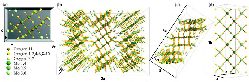
Figure 2: Crystal structure of LiMo₆O₁₇. Li (not shown) is intercalated in the hollows near light-green Mo and light-yellow O atoms. (a) primitive cell spanned by the translation vectors $\mathbf{a},$ $\mathbf{b},$ and $\mathbf{c.}$ Whereas $\mathbf{b}$ is orthogonal to both $\mathbf{c}$ and $\mathbf{a,}$ the latter has a one-per-cent component along $\mathbf{c.}$ The relative lengths of the translation vectors are: $a/b\approx 2.31$ and $c/b\approx\sqrt{3}.$ The primitive cell contains two strings: (Mo3) - Mo2 - Mo1 - Mo4 - Mo5 - (Mo6) and the inverted one: (MO6) - MO5 - MO4 - MO1 - MO2 - (MO3). When we need to distinguish between two equivalent sites (related by inversion), we use upper-case letters for the one in the upper string. Together, the two strings form a bi-string. (b) a 3$\times$3$\times$3 supercell showing $bc$-slabs translated by $\pm\mathbf{a}$. The slabs are separated by Mo3 and Mo6 (light green). (c) A single slab, rotated such that six-fold coordinated Mo (green and dark green) have their bonds to O in the vertical, $z,$ and two horizontal, $x$ and $y,$ directions Eq. (12). Oriented this way, see also Chart (14), the slab forms a staircase running up the $c$-direction, i.e. with the steps translated by $\mathbf{c.}$ A single step is a bi-ribbon formed by translating a bi-string infinitely many times by $\mathbf{b}$. The midpoint between Mo1 and a nearest MO1 in the same bi-ribbon is a center of inversion. The planes perpendicular to $\mathbf{b}$ containing Mo1 and Mo5, as well as those containing Mo4 and Mo2, are mirror planes. The sequence along the vertical, almost straight lines along $\mathbf{z}$ is: (MO6) - Mo5 - MO2 - Mo1 - MO4 - (Mo3) and Li intercalates between the Mo₃O₄ tetrahedron and the MO₃O₄ tetrahedron right above it [2]. (d) 4 primitive cells along $b$ of a single ribbon. Along its center runs the dark-green ${}_{\text{Mo1}}\diagup^{\text{Mo4}}$ zigzag chain. Parallel herewith and shifted by $\mathbf{z}$ [see (c) and Chart (15)] is the partner ribbon with its ${}_{\text{MO4}}\diagup^{\text{MO1}}$ zigzag chain [see also FIG. 1 in Ref. [25]].

III Crystal structure

The crystal structure of LiPB was determined at room temperature and described by Onoda et al [2]. As shown in FIG. 2, there are two LiMo₆O₁₇ units in the primitive cell spanned by the translations $\mathbf{a},$ $\mathbf{b},$ and $\mathbf{c}$ shown in (a). Whereas $\mathbf{b}$ is orthogonal to both $\mathbf{c}$ and $\mathbf{a,}$ the latter has a tiny component along $\mathbf{c.}$ The relative lengths of the primitive translation vectors are: $a/b\approx 2.311$ and $c/b\approx 1.720,$ with $b=5.523\,\mathring{A}.$ We note that in much of the literature, especially experimental papers, an alternate axis labeling [1] is used with the definitions of $a$ and $c$ interchanged. Here we follow Onoda et al. [2]. Since $\mathbf{a},$ $\mathbf{b},$ and $\mathbf{c}$ are nearly orthogonal, so are the primitive translations, $\mathbf{a}^{\ast},$ $\mathbf{b}^{\ast},$ and $\mathbf{c}^{\ast},$ of the reciprocal lattice. They are defined by:

$$\left(\begin{array}[]{ccc}\mathbf{a\cdot a}^{\ast}&\mathbf{a\cdot b}^{\ast}&\mathbf{a\cdot c}^{\ast}\\ \mathbf{b\cdot a}^{\ast}&\mathbf{b\cdot b}^{\ast}&\mathbf{b\cdot c}^{\ast}\\ \mathbf{c\cdot a}^{\ast}&\mathbf{c\cdot b}^{\ast}&\mathbf{c\cdot c}^{\ast}\end{array}\right)\equiv\left(\begin{array}[]{ccc}1&0&0\\ 0&1&0\\ 0&0&1\end{array}\right),$$ (10)

where we use the crystallographic definition of the scale of reciprocal space without the factor $2\pi$ on the right-hand side used in the solid-state definition. The former is traditionally used in diffraction and the latter in spectroscopy. In this paper, we use the crystallographic definition unless otherwise stated. The top of FIG. 3 shows half the Brillouin-zone (BZ) with origin at $\mathrm{\Gamma}$ and spanned by $\pm\frac{\mathbf{a}^{\ast}}{2}$ (B), $\mathbf{\pm}\frac{\mathbf{b}^{\ast}}{2}$ (Y), and $\pm\frac{\mathbf{c}^{\ast}}{2}$ (Z). The Bloch vector,

$$\mathbf{k}=\,k_{a}\mathbf{a}^{\ast}+k_{b}\mathbf{b}^{\ast}+k_{c}\mathbf{c}^{\ast},$$ (11)

is specified by its dimensionless $\left(k_{a},k_{b},k_{c}\right)$-components which, according to Eq.s (10) and (11), are the projections of $\mathbf{k}$ onto respectively $\mathbf{a}$, $\mathbf{b}$, and $\mathbf{c,}$ or equivalently: they are the projections onto the respective directions in units of $a^{-1}$, $b^{-1}$, and $c^{-1}$. Occasionally, we shall use the solid-state definition where the $k$ components are the same, but $\mathbf{a}^{\ast}$, $\mathbf{b}^{\ast}$, $\mathbf{c}^{\ast}$, and $\mathbf{k}$ are $2\pi$ larger, e.g. the Fermi vector for stoichiometric LiPB has length $(\pi/2)b^{-1}=0.2844$ Å^-1 instead of $(1/4)b^{-1}$.

The most relevant symmetry points have $k_{a}$=$0,$ and are: $\left(k_{b},k_{c}\right)$=$\mathrm{Z}\left(0,\frac{1}{2}\right),$ $\mathrm{Y}\left(\frac{1}{2},0\right),$ $\mathrm{\Gamma}\left(0,0\right),$ $\mathrm{C}\left(\frac{1}{2},\frac{1}{2}\right),$ $\mathrm{W}\left(\frac{1}{2},\frac{1}{4}\right),$ $\mathrm{\Lambda}\left(0,\frac{1}{4}\right),$ plus their equivalents. Higher BZs are shifted by reciprocal lattice vectors, $\mathbf{G,}$ which means that $k_{a},$ $k_{b},$ and $k_{c}$ are shifted by integers, which we name respectively $L,$ $M,$ and $N$ and shall use in Sect. VI, and in Sect.s IX.2.1, and X.3 in Paper II.

A simplifying –hitherto overlooked– approximate view of the complicated structure in FIG. 2 is that all Mo atoms are on a lattice spanned by the primitive translations:

$$\frac{\mathbf{c+a}}{6}\mp\frac{\mathbf{b}}{2}\equiv\genfrac{}{}{0.0pt}{}{\mathbf{x}}{\mathbf{y}}\quad\mathrm{and\quad}\frac{\mathbf{c}}{2}\mathrm{-}\frac{\mathbf{c+a}}{6}\equiv\mathbf{z}\,.$$ (12)

These are orthogonal to within a few degrees and their lengths, 3.82 Å, are equal to within 0.3%. This means that all 12 Mo atoms approximately form a simple cubic lattice, 12 times finer than the proper lattice. In FIG. 2 (c), the structure is turned to have $\mathbf{z}$ in the vertical direction, and $\mathbf{x}$ and $\mathbf{y}$ in the horizontal plane. This view is useful for understanding the structure, the computed Wannier orbitals and the measured ARPES, but should not be overstretched. Using for instance the inverse to the transformation (12),

$$\mathbf{a}=2\left(\mathbf{x+y-z}\right),\;\mathbf{b=y-x,\;c}=\mathbf{x+y}+2\mathbf{z,}$$ (13)

and assuming the $xyz$ system to be orthonormal leads to: $a=2\sqrt{3},$ $b=\sqrt{2},$ and $c=\sqrt{6}$ times 3.82 Å, which are wrong by respectively $+$3.7, $-$2.2, and $-$2.1 per cent.

As specified in FIG. 2 (a), of the twelve Mo sites in the primitive cell, six are inequivalent. Four of these (dark-green Mo1 and Mo4, and green Mo2 and Mo5) are six-fold coordinated with oxygen (dark yellow and yellow) in the $\pm x$, $\pm y$, and $\pm z$ directions and form a network of corner-sharing MoO₆ octahedra. We shall call them octahedral molybdenums. The remaining two types of Mo (light-green Mo3 and Mo6) are four-fold coordinated with oxygen (yellow and light yellow). The latter, tetrahedrally coordinated Mo atoms (light green, set in parentheses in the following) form double layers, which separate the network of corner-sharing MoO₆ octahedra into slabs. The crystals cleave between slabs.

Such a slab has the form of a staircase with steps of bi-ribbons stacked with period $\mathbf{c}$ as seen in FIG. 2 (c). Schematically, this is:

$$\begin{array}[]{cc}&\\ &\\ \mathbf{c}&\nearrow\\ \mathbf{a}&\searrow\\ \mathbf{z}&\uparrow\\ &\\ &\end{array}\,\framebox{{\hbox{\begin{array}[]{ccccccccc}\mathbf{2}&1&\mathbf{4}&5&&&\mathbf{2}&1&\mathbf{4}\\ \mathbf{1}&2&&&\mathbf{5}&4&\mathbf{1}&2&\\ \mathbf{4}&5&&&\mathbf{2}&1&\mathbf{4}&5&\\ &&\mathbf{5}&4&\mathbf{1}&2&&&\mathbf{5}\\ &&\mathbf{2}&1&\mathbf{4}&5&&&\mathbf{2}\\ \mathbf{5}&4&\mathbf{1}&2&&&\mathbf{5}&4&\mathbf{1}\\ \mathbf{2}&1&\mathbf{4}&5&&&\mathbf{2}&1&\mathbf{4}\end{array}}}},$$ (14)

where the octahedral molybdenums lying in the same $ac$-plane are either normal- or bold-faced. The distance between such $ac$-planes is $\frac{\mathbf{b}}{2}.$ A single ribbon is four octahedral molybdenums wide and, as seen here:

$${\begin{array}[]{cc}&\\ \mathbf{b}&\uparrow\\ \mathbf{c+a}&\longrightarrow\\ \mathbf{y}&\nearrow\\ \mathbf{x}&\searrow\\ &\end{array}}\,{\begin{array}[]{cc}\mathrm{Mo:}&\mathrm{MO:}\\ \framebox{$\begin{array}[]{cccccc}&2&&4&&\\ &&1&&5&\\ &2&&4&&\\ &&1&&5&\\ &2&&4&&\\ &&1&&5&\end{array}$}&\,\framebox{$\begin{array}[]{cccccc}&5&&1&&\\ &&4&&2&\\ &5&&1&&\\ &&4&&2&\\ &5&&1&&\\ &&4&&2&\end{array}$}\end{array}},$$ (15)

and in FIG.s 2 (c) and (d), extends indefinitely in the $b$-direction and lies in the horizontal $xy$-plane containing the vectors $\mathbf{b=y-x}$ and $\mathbf{c+a=}$ $3(\mathbf{x+y})$. The lower half of a bi-ribbon, seen in the left-hand panel of Chart (15), consist of (Mo3) - Mo2 - Mo1 - Mo4 - Mo5 - (Mo6) strings separated by $\mathbf{b}$ and can be taken either as a zigzag line changing translation between $\mathbf{y}$ and $\mathbf{x,}$ and thus running along $\mathbf{c+a}$, or as a nearly straight line running along $\mathbf{x,}$ or as one running along $\mathbf{y}$ [see (d) and (15)]. In the following, we shall refer to these as respectively $\left(\mathbf{c+a}\right)$-zigzag, $\mathbf{x}$-, and $\mathbf{y}$ strings.

The upper ribbon is shown to the right in Chart (15). Its Mo sequence, (MO6) - MO5 - MO4 - MO1 - MO2 - (MO3), is inverted such that e.g. MO4 is on top of Mo1. When we need to distinguish between two equivalent sites related by inversion in their midpoint –a center of inversion for the entire crystal– we use upper-case letters for the one in the upper ribbon.

Note that the $\left(\mathbf{c+a}\right)$-zigzag string is different from –and perpendicular to– the $\diagdown_{\text{Mo1}}\diagup^{\text{Mo4}}\diagdown$ zigzag chain along $\mathbf{b},$ the backbone of the electronic 1D $xy$-band shown in FIG. 1 of Ref. [25] together with its partner $\diagdown_{\text{MO4}}\diagup^{\text{MO1}}\diagdown$ in the upper ribbon.

III.1 $c$-dimerization

The vectors from Mo1 to its two nearest MO1 neighbors inside and outside the bi-ribbon are respectively $\frac{\mathbf{c\pm b}}{2}-\mathbf{d}$ and $-\left(\frac{\mathbf{c\pm b}}{2}+\mathbf{d}\right)$ where

$$\mathbf{d}=0.012\mathbf{a}+0.033\mathbf{c}$$ (16)

is the displacement dimerization. Hence, the distances measured along $\mathbf{c}$ from a ribbon to its neighbors inside and outside the bi-ribbon are respectively 6.6% smaller and 6.6% larger than the average distance $\frac{c}{2}.$

Due to the stacking (14) into a staircase of bi-ribbons, Mo4 differs from Mo1, and Mo5 differs from Mo2, in having no neighbor belonging to the next bi-ribbon, i.e., they have only one octahedral Mo neighbor along $z.$ As seen in Charts (14) and (15), Mo1 has six, Mo4 five, Mo2 four, and Mo5 three nearest Mo neighbors which are octahedrally coordinated with oxygen.

In the next section, we shall explain –and later demonstrate by computation and experiment– that the six lowest energy bands are described by the six planar $t_{2g}$ Wannier orbitals (WOs), $w_{m}\left(\mathbf{r}\right)$ and $W_{m}\left(\mathbf{r}\right)$ $\left(m\mathrm{=}xy,xz,yz\right),$ centered on respectively Mo1 and on MO1. These sites, separated by $\frac{\mathbf{c+b}}{2}-\mathbf{d,}$ are special in having a full nearest-neighbor shell of octahedral molybdenums and therefore best preserve the $t_{2g}$ symmetry of the WO and are least sensitive to the steps of the staircase, the second cause for the dimerization. Such a WO (FIG. 9) spreads substantially onto the four nearest Mo neighbors in the orbital’s plane with amplitudes falling in the same order as the above-mentioned Mo coordination of those neighbors. As a result of this, and the smallness of the displacement dimerization (16), the two $t_{2g,m}$ WOs are approximately related by half a lattice translation:

$$W_{m}\left(\mathbf{r-}\frac{\mathbf{c+b}}{2}\right)~{}\approx~{}w_{m}\left(\mathbf{r}\right).$$ (17)

However, the exact relation is:

$$W_{m}\left(\mathbf{r-}\frac{\mathbf{c+b}}{2}+\mathbf{d}\right)=w_{m}\left(-\mathbf{r}\right),$$ (18)

and its differences, $W_{m}\left(\mathbf{r-}\frac{\mathbf{c+b}}{2}+\mathbf{d}\right)-W_{m}\left(\mathbf{r-}\frac{\mathbf{c+b}}{2}\right)$ and $w_{m}\left(-\mathbf{r}\right)-w_{m}\left(\mathbf{r}\right),$ to the approximate relation (17) will be referred to as respectively the displacement- and the inversion dimerization.

A consequence of the approximate translational equivalence (17), which may be seen to hold far better for the $xy$- than for the $xz$- and $yz$ WOs, is that the low-energy band structure, $E_{j}\left(\mathbf{k}\right)$ with $j$=1-6 (e.g. FIG. 6), approximately consists of 3 bands, $E_{m}\left(\mathbf{k}\right),$ one with each $m$-character, and extending in a double zone of the sparse reciprocal sublattice spanned by

$$\left(\mathbf{a}^{\ast},\,\mathbf{c}^{\ast}+\mathbf{b}^{\ast},\,\mathbf{c}^{\ast}-\mathbf{b}^{\ast}\right).$$ (19)

This is the reciprocal of the un-dimerized lattice spanned by

$$\left(\mathbf{a,}\,\frac{\mathbf{c+b}}{2},\,\frac{\mathbf{c-b}}{2}\right)=\left(\mathbf{a,\,y+z},\,\mathbf{x+z}\right)$$ (20)

with only one LiMo₆O₁₇ unit per primitive cell. The two last translations (20), we shall call pseudo translations. If expression (17) were true, the $E_{m}\left(\mathbf{k}\right)$ band would be equivalent to the one translated by (any odd number times) $-\mathbf{c}^{\ast},$ e.g. with $E_{m}\left(\mathbf{k+c}^{\ast}\right),$ but the presence of the inversion- and displacement dimerizations, (18) and (16), cause these two bands to gap where they cross, i.e. at the boundaries of the small zones. The resulting band structure is periodic in the proper (small) zone, corresponding to the proper primitive cell with two LiMo₆O₁₇ units, and has six continuous bands, two for each $m,$ of which the lower is approximately $E_{m}\left(\mathbf{k}\right)$ and the higher is approximately $E_{m}\left(\mathbf{k+c}^{\ast}\right)$ in the odd-numbered zones; and the other way around in the even-numbered zones. As we shall see in Paper II, ARPES approximately sees only the $E_{m}\left(\mathbf{k}\right)$-like band, i.e. both bands, but separated in zones, and this will allow us to resolve the splitting and the perpendicular dispersion of the two quasi-1D bands in the gap.

The un-dimerized lattice has one LiMo₆O₁₇ unit per primitive cell and is spanned by the primitive translations (20) where, on the right-hand side, we have used the approximate relation (13). This shows that the un-dimerized lattice is 2D and hexagonal in the planes perpendicular to $\mathbf{a.}$ This is the structure of the purple bronzes isoelectronic with LiPB, NaMo₆O₁₇ and KMo₆O${}_{17},$ where CDW fluctuations with wavevector $\mathbf{c}^{\ast}$ have been observed below 120 K and have been explained as driven by the simultaneous gapping of the 1D $xz$- and the $yz$ Fermi-surface (FS) sheets by one and the same nesting vector, $\mathbf{c}^{\ast}$ [30, 65]. The lattice reciprocal to the un-dimerized one is spanned by (19), and its BZ is the double zone of the dimerized structure, i.e. that of LiPB shown in FIG. 8. Hence, we may consider the structure of quasi-1D LiPB as the CDW dimerization of quasi-2D Na- or KPB, whose electronic structure consists of the 1D $xy$-, $yz$-, and $xz$-bands dispersing at 120^∘ relatively to each other in the plane perpendicular to $\mathbf{a}$. The reason why not also the $xy$ FS sheets gap away is that relation (17) holds much better for the $xy$ WOs than for the $xz$ and $yz$ WOs.

For comparison with Charts (14) and (15), the un-dimerized slab is:

$$\begin{array}[]{cc}&\\ &\\ \mathbf{c}&\nearrow\\ \mathbf{a}&\searrow\\ \mathbf{z}&\uparrow\\ &\\ &\end{array}\,\framebox{{\hbox{\begin{array}[]{ccccccccc}\mathbf{4}&1&\mathbf{2}&&&5&\mathbf{4}&1&\mathbf{2}\\ \mathbf{1}&2&&&\mathbf{5}&4&\mathbf{1}&2&\\ \mathbf{4}&&&5&\mathbf{4}&1&\mathbf{2}&&\\ &&\mathbf{5}&4&\mathbf{1}&2&&&\mathbf{5}\\ &5&\mathbf{4}&1&\mathbf{2}&&&5&\mathbf{4}\\ \mathbf{5}&4&\mathbf{1}&2&&&\mathbf{5}&4&\mathbf{1}\\ \mathbf{4}&1&\mathbf{2}&&&5&\mathbf{4}&1&\mathbf{2}\end{array}}}},$$ (21)

where the steps of the staircase are smoothed out to a ramp, and the two ribbons are identical:

$${\begin{array}[]{cc}&\\ \mathbf{b}&\uparrow\\ \mathbf{c+a}&\longrightarrow\\ \mathbf{y}&\nearrow\\ \mathbf{x}&\searrow\\ &\end{array}}{\begin{array}[]{cc}\mathrm{Mo:}&\mathrm{MO:}\\ \,\framebox{$\begin{array}[]{cccccc}&&4&&2&\\ &5&&1&&\\ &&4&&2&\\ &5&&1&&\\ &&4&&2&\\ &5&&1&&\end{array}$}&\framebox{$\begin{array}[]{cccccc}&&5&&1&\\ &&&4&&2\\ &&5&&1&\\ &&&4&&2\\ &&5&&1&\\ &&&4&&2\end{array}$}\end{array}}$$ (22)

III.2 $b$-dimerization

An unrelated and different dimerization is the one known from the description of the 1D band structure as two, approximately 4 eV broad, $\frac{1}{4}$-filled $xy$ bands [FIG. 3 and Eq.s (23)-(24)] running on zigzag chains along $\mathbf{b}$ [24,25] and with the nearest neighbor Mo1-Mo4 hopping integral $t\sim-1$ eV. In this view, Mo1 and Mo4 are inequivalent because of a dimerization from $\frac{\mathbf{b}}{2}$ to $\mathbf{b}$. In reciprocal space, this dimerization is from $2\mathbf{b}^{\ast}$ to $\mathbf{b}^{\ast}$ and causes gaps at $k_{b}=\pm\frac{1}{2}\approx\pm 2k_{F}$ which separate the broad $xy$ bands into two lower $\frac{1}{2}$-filled and two higher empty bands. The two latter bands will not be described by our set of six WOs, which are essentially Mo1-Mo4 bonding orbitals (FIG. 9), but would require the inclusion of also Mo1-Mo4 anti-bonding orbitals, thus leading to a basis set unpractically large for our purpose of understanding the photoemission from the occupied bands.

IV Basic electronic structure

Shortly after the structural determination, Whangbo and Canadell [24] used the extended Hückel method to calculate and explain the basic electronic structure, but it took almost twenty years before a charge-self-consistent calculation could be performed. This was done by Popović and Satpathy [25] who used the LDA-DFT and the LMTO method. In the following, we shall explain and expand on these works using the insights gained from the view of the structure given in the previous section and from the results of the WO calculations to be presented in Sect.s V and VI.

In FIG. 3, we show the LDA energy bands over a range of $\pm 9$ eV around the Fermi level, together with their density of states projected onto O (green) and onto tetrahedrally- (blue) and octahedrally- (red) coordinated Mo. The bands between $-8$ and $-2$ eV have predominantly O $2p$ character and those extending upwards from $B\sim-$0.7 eV predominantly Mo $4d$ character and, above +0.8 eV, also Mo $5s$ and $5p$ characters. The states in the O $2p$ band are bonding linear combinations with Mo $5s,5p,$ and $4d$ orbitals, the more bonding, the lower their energy. The states in the Mo $4d$ band are anti-bonding linear combinations with O $2s$ and $2p$ orbitals; the more anti-bonding, the higher their energy.

The 2 eV gap between the O $2p$-like and Mo $4d$-like bands is –for the purpose of counting– ionic with Li donating one and Mo six electrons to- and O acquiring two electrons from the Mo$\,4d$-like bands above the gap, which thereby hold 2$\left(1+6\times 6-17\times 2\right)$ $=6$ electrons per 2(LiMo₆O₁₇). Had this charge been spread uniformly over all molybdenums, this would correspond to a Mo $d^{0.5}$ occupation.

Figure 3: The top shows half ($k_{c}\geq 0$) the (1st) Brillouin-zone of LiMo₆O₁₇ with the labeling of the symmetry points for P2₁/m obtained from the Bilbao crystal server [66]. The most relevant symmetry points have $k_{a}$=$0$ and are: $\left(k_{b},k_{c}\right)$=$\mathrm{\Gamma}\left(0,0\right),$ $\mathrm{Y}\left(\frac{1}{2},0\right),$ $\mathrm{W}\left(\frac{1}{2},\frac{1}{4}\right),$ $\mathrm{C}\left(\frac{1}{2},\frac{1}{2}\right),$ $\mathrm{Z}\left(0,\frac{1}{2}\right),$ $\mathrm{\Lambda}\left(0,\frac{1}{4}\right),$ and their equivalents. Below is the LDA band-structure calculated with the large basis set of 336 NMTOs (left) and its partial densities of states (right) over a wide energy range. The zero of energy is the Fermi level of the stoichiometric compound.

The $4d$ orbitals forming the most anti-bonding and bonding states with O are the $e_{g}$ orbitals, $3z^{2}-1$ and $x^{2}-y^{2},$ on the octahedrally coordinated Mo because their lobes point towards the two O neighbors along $z$ and the four O neighbors in the $xy$ plane, respectively, and thereby form $pd\sigma$ bonds and anti-bonds. Not only the $e_{g}$ orbitals on the octahedrally coordinated Mo, but all $4d$ orbitals ($t$ and $e)$ on the tetrahedrally coordinated Mo form filled bonding and empty anti-bonding states with their O neighbors, and thereby contributing to the stability of the crystal. However, as seen from the projected densities of states in FIG. 3, none of them contribute to the LDA bands within an eV around the Fermi level, which are the ones of our primary interest. So as long as there are no additional perturbations or correlations with energies in excess of this, which is assumed in the $\frac{1}{2}$-filled models, the Mo $t$ and $e$ orbitals are uninteresting for the low-energy electronics, and so are the Li $2s$ orbitals which contribute two bands several eV above the Fermi level, mix a bit with the oxygen states several eV below $E_{F}$, and donate their two electrons to them. Due to the Pauli principle, changing the Li content (doping) will change the position of the Fermi level, which is inside the Mo $t_{2g}$ bands.

Although the MoO₄ tetrahedra do not contribute any electrons near the Fermi level, their arrangement in double layers perpendicular to $\mathbf{a,}$ separating the staircases of corner-sharing octahedra, has an important impact on the low-energy electronic structure: It suppresses the hopping between the low-energy orbitals across the double layer to the extent that we shall neglect it in our TB model for the six lowest bands.

IV.1 The $t_{2g}$ bands

The remaining $4d$ orbitals on octahedrally coordinated Mo are the $t_{2g}$ orbitals, $xy,$ $xz,$ and $yz,$ whose lobes point between the four O neighbors in respectively the $xy,$ $xz,$ and $yz$ planes and therefore form relatively weak $pd\pi$ bonds and antibonds, e.g. $\mathrm{Mo}\,xy\pm\mathrm{O}\,y$ on the $\frac{\mathbf{x}}{2}$ bond. Whereas the bonds are dominated by oxygen and form bands that are part of the O $2p$ continuum below about $-4$ eV, the antibonds are dominated by Mo and form $4\times 2\times 3=24$ bands which extend from $+3.0~{}$eV down to the bottom of the Mo $4d$ continuum at $-$0.7 eV. This spread in energy is conventionally described as due to hopping between dressed Mo$\,t_{2g}$ orbitals, where the dressing consists of the $pd\pi$ anti-bonding tails on the four oxygens in the plane of the orbital. Since the dressed orbitals are planar, the strongest hoppings are between like $t_{2g}$ orbitals which are nearest neighbors in the same plane, e.g. as seen in the right-hand panel of FIG. 5 between the dressed $xy$ orbital on Mo1${}_{\text{{o}}}$ and those on Mo4${}_{\mathbf{x}},$ Mo4_y, Mo2${}_{\mathbf{-x}},$ and Mo2_-y , or as seen in the left-hand panel between the dressed $yz$ orbital on Mo1_o and those on Mo4${}_{\mathbf{y}},$ Mo4_z, Mo2${}_{\mathbf{-y}},$ and Mo2_-z. These hoppings are $dd\pi$-like and of magnitude $t=-1~{}$eV.

The main dispersion of the $xy$ band is, therefore, in the direction of the $xy$ lobe pointing along $\mathbf{y-x}=\mathbf{b,}$ that of the $yz$ band is in the direction of the $yz$ lobe pointing along $\mathbf{y+z=}\frac{\mathbf{c+b}}{2}\mathbf{\ }$(see left-hand FIG. 5), and that of the $xz$ band is in the direction of the $xz$ lobe pointing along the $\mathbf{x+z=}\frac{\mathbf{c-b}}{2};$ see Charts (14) and (15)

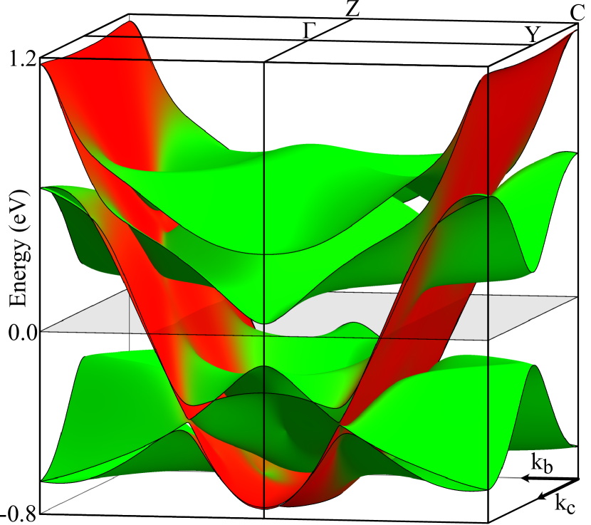
Figure 4: LDA $t_{2g}$ energy band structure and Fermi level of LiPB at half filling. Red and green colors indicate respectively $xy$ and $xz/yz$ characters. The energy region is from 0.8 eV below to 1.2 eV above $E_{F}$ (see FIG.  3) and the $\mathbf{k}$-space region is the BZ (see FIG.  8). The LDA TB parameters listed in Tables (43)-(47) were used, like in FIG.  22 (a) in Paper II.

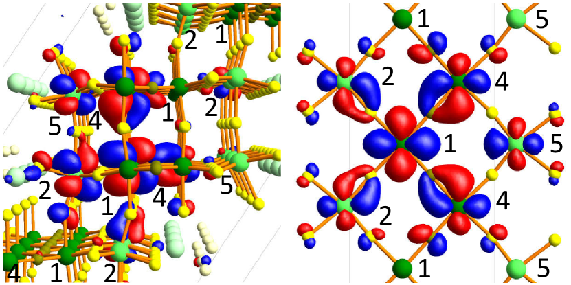
Figure 5: Left: $yz$ standing-wave state with $k_{c}+k_{b}=$ $\pm\frac{1}{2}$ which behaves like $\cos 2\pi\frac{1}{2}\left(r_{c}+r_{b}\right).$ View along $\mathbf{b}$ as in FIG. 2 (c) and Chart (14). Right: $xy$ standing-wave state with $\left|k_{b}\right|=$ $\frac{1}{4}\sim k_{F}$ which behaves like $\cos 2\pi\frac{1}{4}r_{b}.$ View along $-\mathbf{z\sim a-c}$ as in (d) and Chart (15). The sign of a lobe is indicated by its color. See also FIG. 9 with caption. As explained in Sect. VI, these figures are identical with those shown in FIG.  9 of the $yz$ and $xy$ Wannier Orbitals (WOs) on site 1. The $xy$ WO has a halo consisting of $xy$ partial waves on the four nearest Mo-neighbor sites, 4 and 2, plus a weaker one on the next-nearest Mo-neighbor site 5. The $yz$ WO has a halo consisting of $yz$ patial waves (of unequal magnitude) on the two nearest-Mo neighbor sites 4, plus weaker ones on Mo2 and 5.

IV.1.1 The four $xy$ bands.

The right-hand panel of FIG. 5 shows the $xy$ standing-wave state with $\left|k_{b}\right|$=$\frac{1}{4}\sim k_{F}$ which behaves like $\cos 2\pi k_{b}\mathbf{b}^{\ast}\mathbf{\cdot b}r_{b}\equiv$ $\cos 2\pi\frac{1}{4}r_{b},$ i.e. is even around the $\mathbf{c+a}$ line through Mo1 and Mo5 and has nodes at the Mo1-Mo5 lines translated by $\pm\mathbf{b}$. Here, the orientation is like in FIG. 2 (d) with the Mo numbering given in the left-hand panel of Chart (15). We see that the amplitudes of the dressed $xy$ orbitals are largest at Mo1 and decrease in the order Mo4, Mo2, and Mo5, thus following the decrease of the Mo coordination mentioned in Sect. III.1. The dressed orbitals on the four nearest neighbors (Mo4 at $x$ and $y,$ and Mo2 at $-x$ and $-y$) anti-bond to the central orbital, i.e. nearest-neighbor lobes have different colors. This is the reason why the overlap from the neighboring dressed $xy$ orbital weakens the O $y$ (or $x$) amplitude on the common oxygen such that its contour merges with that of the weaker Mo neighbor. Hence, O $p$ is $pd\pi$ anti-bonding with Mo1$\,xy$ and bonding with Mo4$\,xy$ and Mo2$\,xy.$ The net result is $pd\pi$ non-bonding, essentially.

The $xy$ band disperses almost exclusively in the $\mathbf{b}$ direction, and now, we imagine going to the $xy$ state with $\left|k_{b}\right|$=$\frac{3}{4}$=$\frac{1}{4}\left[\mathrm{mod}\frac{1}{2}\right]$ and energy $\sim$2.8 eV above $E_{F},$ i.e. to the state in the next $xy$ band. Here, the signs (colors) of the dressed $xy$ orbitals on the four nearest neighbors (Mo4 and Mo2) will have changed, whereby the overlaps on the common oxygens shared with Mo1 will have their amplitudes enhanced and the O$\,y$ (or $x$) contour will be separated by a node, not only from the stronger Mo1-$xy$ contour, but also from the weaker Mo4-$xy$ (or Mo2-$xy)$ contour. In the following, we shall refer to the $xy$ band with the lower/higher energy as the Mo1-Mo4 bonding/anti-bonding band, although both of these bands are $pd\pi$ non- or anti-bonding; but the one with the lower energy has fewer $pd\pi$ nodes.

The dressed $xy$ orbitals lie in the plane of a ribbon, and those along the infinite zigzag chain, $\overset{\mathbf{-x}}{\rightarrow}$ Mo1 $\overset{\mathbf{y}}{\rightarrow}$ Mo4 $\overset{\mathbf{-x}}{\rightarrow}$, with pseudo translation $\frac{\mathbf{y-x}}{2}\mathrm{=}\frac{\mathbf{b}}{2}$ form the well-known [24][25][17] quasi-1D band with dispersion:

$$\varepsilon_{xy}\left(\mathbf{k}\right)\sim 2t\cos\left(2\pi\mathbf{k}\cdot\frac{\mathbf{b}}{2}\right)=2t\cos\pi k_{b},$$ (23)

where $t\sim-1~{}$eV. Since $\mathbf{b,}$ and not $\frac{\mathbf{b}}{2},$ is the proper lattice translation because Mo1 and Mo4 are not equivalent, the band must be folded from the large BZ bound by the midplanes $\left(k_{b}\text{=}\pm\text{1}\right)$ of the reciprocal-lattice vectors $\pm 2\mathbf{b}^{\ast},$ into the proper, small BZ bound by the midplanes $\left(k_{b}=\pm\frac{1}{2}\right)$ of $\pm\mathbf{b}^{\ast}$ whereby it becomes $-2t\cos\pi k_{b}.$ An equivalent prescription –more useful than BZ-folding, as we shall see below for the bonding $yz$ and $xz$ bands,– is to say that if $\mathbf{k}$ must be limited to the proper, small BZ, then we must also consider the band,

$$\varepsilon_{xy}\left(\mathbf{k+b}^{\ast}\right)\sim 2t\cos\left[\pi\left(k_{b}+1\right)\right]=-2t\cos\pi k_{b},$$ (24)

translated by the proper reciprocal lattice vector, $-\mathbf{b}^{\ast}.$ Finally, the inequivalence of –or ”dimerization into”– Mo1 and Mo4, couples the $xy\left(\mathbf{k}\right)$ and $xy\left(\mathbf{k+b}^{\ast}\right)$ bands, and where they are degenerate –which is for $\left|k_{b}\right|$=$\frac{1}{2},$ i.e. at the boundaries of the proper BZ (YC)– they are gapped by $\pm$0.3 eV. Since this gap is relatively large, the $xy\left(\mathbf{k}\right)$ band is bonding and the $xy\left(\mathbf{k+b}^{\ast}\right)$ band anti-bonding between Mo1 and Mo4 for $\mathbf{k}$ inside the proper BZ. The latter, empty $xy$ band, which extends from approximately 1.7 to 3.4 eV above $E_{F},$ we shall neglect in the bulk of the present papers, as was already mentioned in Sect. III.2.

Degenerate and parallel with the Mo1-Mo4 bonding and anti-bonding $xy$ bands running along the lower ribbon are MO4-MO1 bonding and anti-bonding $XY$ bands running along the upper ribbon [see FIG. 2 (d), Chart (14), and the right-hand panel of Chart (15)]. Their $\left|k_{b}\right|$=$\frac{1}{4}\sim k_{F}$ standing-wave state looks like the one shown on the right-hand side of FIG. 5, but has MO1 on top of Mo4 and vice versa. Viewed along $\mathbf{b,}$ the appearance of the $xy$ and $XY$ states is like that of the $xy$ and $XY$ WOs in the first two columns on the top row of FIG. 9. From there, we realize that these flat, parallel states are well separated, each one on its own ribbon, with no contribution on the oxygens in between. The $dd\delta$-like hops between the $xy$ and $XY$ orbitals inside the same bi–ribbon $\left(t_{\perp}\equiv t_{1}+u_{1}\sim-14\,\mathrm{meV}\right)$ and between the $XY$ and $xy$ orbitals in different bi-ribbons $\left(t_{\perp}^{\prime}\equiv t_{1}-u_{1}\sim-8\,\mathrm{meV}\right),$ give the bands a perpendicular ($k_{c}$-)  dispersion, which is two orders of magnitude smaller than the $k_{b}$-dispersion given by Eq. (23). If all ribbons were translationally equivalent, i.e. if the primitive translations (neglecting $\mathbf{a)}$ were $\mathbf{x+z}=\frac{\mathbf{c-b}}{2}$ and $\mathbf{y+z=}\,\frac{\mathbf{c+b}}{2}$ with reciprocal-lattice translations $\mathbf{c}^{\ast}\mathbf{-b}^{\ast}$ and $\mathbf{c}^{\ast}+\mathbf{b}^{\ast},$ the $dd\delta$ hopping would add

$$2t_{1}\left[\cos\pi\left(k_{c}-k_{b}\right)+\cos\pi\left(k_{c}+k_{b}\right)\right]=4t_{1}\cos\pi k_{b}\cos\pi k_{c}$$

to Eq. (23). But since the primitive translations are really $\mathbf{b}$ and $\mathbf{c,}$ we must –if we want to confine $\mathbf{k}$ to the proper BZ– also add the equivalent term translated by the proper reciprocal lattice vector, $-\mathbf{c}^{\ast}.$ As a result, we get for the two $\frac{1}{2}$-filled $xy$ bands:

$$\varepsilon_{xy}\left(\begin{array}[]{c}\mathbf{k}\\ \mathbf{k+c}^{\ast}\end{array}\right)\sim 2t\left[1\pm\left(2t_{1}/t\right)\cos\pi k_{c}\right]\cos\pi k_{b},$$ (25)

where the distortion caused by the gap extending upwards from $\sim 1.1~{}$eV above $E_{F}$ has been neglected. As long as $\mathbf{k}$ is inside the 1st BZ $\left(\left|k_{c}\right|\leq\frac{1}{2}\right),$ the $xy\left(\mathbf{k}\right)$ band is bonding and the $xy\left(\mathbf{k+c}^{\ast}\right)$ band anti-bonding between ribbons, i.e. between $xy$ and $XY.$ In the 2nd BZ $\left(\left|k_{c}-1\right|\leq\frac{1}{2}\right),$ the opposite is true (see FIG. 6). The translational inequivalence of the two ribbons –i.e. the dimerization into bi-ribbons– finally splits the degeneracy of the $xy\left(\mathbf{k}\right)$ and $xy\left(\mathbf{k+c}^{\ast}\right)$ bands at the BZ boundaries $\left|k_{c}\right|$=$\frac{1}{2}$ (the ZCED planes) by $\pm 2\sqrt{2}u_{1}\cos\pi k_{b},$ which for $k_{b}$=$\frac{1}{4}\sim k_{F}$ is a mere $\pm 8~{}$meV.

IV.1.2 The two $yz$ and the two $xz$ bands.

In the planes perpendicular to the bi-ribbons [FIG. 2 (c) and Chart (14)] and cutting them along the $\mathbf{y}$-strings [FIG. 2 (d) and Chart (15)], lie the dressed $yz$ orbitals, and in the planes cutting along the $\mathbf{x}$-strings, lie the dressed $xz$ orbitals. The left-hand panel of FIG. 5 shows that $\left|k_{c}+k_{b}\right|$=$\frac{1}{2}$ standing-wave state of the $yz$ band which behaves like $\cos 2\pi\frac{1}{2}\left(r_{c}+r_{b}\right),$ i.e. is even around the Mo1-containing planes which are perpendicular to $\mathbf{c}^{\ast}+\mathbf{b}^{\ast}$ and has nodes in the MO1-containing planes. Like for $xy$ state in the right-hand panel, the dressed $yz$ orbitals on the four nearest neighbors in the plane of the orbital (MO4 at $\mathbf{z}$, Mo4 at $\mathbf{y,}$ Mo2 at $-\mathbf{y}$, and MO2 at $-\mathbf{z}$) are $dd\pi$ anti-bonding with the dressed $yz$ on the central Mo1, which means $pd\pi$ non-bonding with the oxygen. Here again, the amplitudes of the dressed $yz$ orbitals decrease like the Mo coordination.

Whereas in the plane of the $xy$ orbital, Mo4 –like Mo1– has four nearest neighbors of molybdenums coordinated octahedrally with oxygen, in the plane of the $yz$ orbital, Mo4 has only three neighbors, and so does Mo2, while Mo5 has merely two. As noted in Sect. III.1, this is due to the stacking into a staircase of bi-ribbons (14). As a result, the $yz$ orbitals on the Mo1- and MO1-sharing zigzag double chain,

$$\begin{array}[]{cc}\mathbf{c}&\nearrow\\ \mathbf{a}&\searrow\\ \mathbf{z}&\uparrow\end{array}\,\framebox{{\hbox{\begin{array}[]{cccccc}&&\mathbf{5}&\rightarrow 4&\mathbf{\uparrow 1\rightarrow}&2\uparrow\\ &&\mathbf{\rightarrow 2}&\uparrow 1\rightarrow&\uparrow\mathbf{4}&5\\ \mathbf{5}&\rightarrow 4&\mathbf{\uparrow 1\rightarrow}&2\uparrow&&\\ \mathbf{\rightarrow 2}&\uparrow 1\rightarrow&\mathbf{4\uparrow}&5&&\end{array}}}},$$ (26)

running up the staircase with pseudo translation $\mathbf{z+y}=\frac{\mathbf{c+b}}{2},$ form a quasi-1D band dispersing like

$$\varepsilon_{yz}\left(\mathbf{k}\right)=2A_{1}\cos\left(2\pi\mathbf{k\cdot}\frac{\mathbf{c+b}}{2}\right)=2A_{1}\cos\pi\left(k_{c}+k_{b}\right),$$ (27)

with an effective hopping integral, $A_{1}\sim-0.3$ eV and bandwidth 4$\left|A_{1}\right|\sim 1.2$ eV. Because the hopping between ribbons proceeds via Mo4 inside the bi-ribbon, but via Mo2 between bi-ribbons, and because the former distance is shorter than the latter, the hopping integrals are different, respectively $A_{1}+G_{1}\sim-0.3-0.1\sim$ $-0.4$ eV and $A_{1}-G_{1}\sim$ $-0.2$ eV. This dimerization into bi-ribbons causes $\mathbf{c,}$ rather than $\frac{\mathbf{c+b}}{2},$ to be a primitive lattice translation whereby the $yz\left(\mathbf{k}+\mathbf{c}^{\ast}\right)$ band with dispersion

$$\varepsilon_{yz}\left(\mathbf{k+c}^{\ast}\right)=-2A_{1}\cos\pi\left(k_{c}+k_{b}\right)$$ (28)

is equivalent to the $yz\left(\mathbf{k}\right)$ band (27). Where these bands are degenerate, i.e. for $\left|k_{c}+k_{b}\right|$=$\frac{1}{2},$ they gap by $\pm 2\left|G_{1}\right|\sim\pm 0.2~{}$eV whereby they become:

$$\varepsilon_{yz}=\pm\sqrt{\left[2A_{1}\cos\pi\left(k_{c}+k_{b}\right)\right]^{2}+\left[2G_{1}\sin\pi\left(k_{c}+k_{b}\right)\right]^{2}}.$$ (29)

For $\mathbf{k}$ between the $\left|k_{c}+k_{b}\right|$=$\frac{1}{2}$ planes, the $yz\left(\mathbf{k}\right)$ and $yz\left(\mathbf{k+c}^{\ast}\right)$ bands are respectively bonding and anti-bonding between neighboring ribbons. The two $yz$ bands, decorated by the $\mathbf{k}$-character (27), are shown in green in FIG. 6.

It should be noted that the gapping takes place for $\left|k_{c}+k_{b}\right|$=$\frac{1}{2},$ which is not at the boundary of the conventional BZ, $\left|k_{b}\right|$=$\frac{1}{2}$ and $\left|k_{c}\right|$=$\frac{1}{2}$ shown in FIG.s 3 and 8, but where the $\varepsilon_{yz}\left(\mathbf{k}\right)$ and $\varepsilon_{yz}\left(\mathbf{k+c}^{\ast}\right)$ bands are degenerate. Nevertheless, the zone centered at $\Gamma\left(0,0\right)$ and bound by the planes $\left|k_{b}\right|$=$\frac{1}{2}$ and $\left|k_{c}+k_{b}\right|$=$\frac{1}{2}$ (ZYAD) is a primitive cell of the reciprocal lattice, and we call it a physical zone, useful for understanding properties of the $yz$ bands.

With the substitution: $\mathbf{b}\rightarrow\mathbf{-b},$ everything said about the $yz$ bands holds for the $xz$ bands (shown in blue in FIG. 6).

As regards choices of zones, we can either take:

$$\left|k_{b}\right| \leq \frac{1}{2}\;\mathrm{and}\;\left|k_{c}\right|\leq\frac{1}{2},$$ (30)

$$\left|k_{b}\right| \leq \frac{1}{2}\;\mathrm{and}\;\left|k_{c}+k_{b}\right|\leq\frac{1}{2},$$ (31)

$$\mathrm{or\;}\left|k_{b}\right| \leq \frac{1}{2}\;\mathrm{and}\;\left|k_{c}-k_{b}\right|\leq\frac{1}{2},$$ (32)

but not $\left|k_{c}+k_{b}\right|\leq\frac{1}{2}$ and $\left|k_{c}-k_{b}\right|\leq\frac{1}{2}$ whose volume (area) is only half the BZ volume (see FIG. 8). Expressions (30)-(32) thus define the physical zones for respectively the $xy,$ the $yz,$ and the $xz$ bands.

Figure 6: The six pure-$m$ $t_{2g}$ bands ($m=yz$ green, $xz$ blue, and $xy$ red) as functions of $k_{c}$ in the double zone $\left(-1<k_{c}\leq 1\right)$ and for $k_{b}$=0.225, i.e. along the brown dot-dashed line containing P and Q in FIG. 8. 10% hole doping will place the Fermi level inside the red bands. The $m\left(\mathbf{k}\right)$ and $m\left(\mathbf{k+c}^{\ast}\right)$ bands, whose dispersions are described in Sect. IV.1, have period $\Delta k_{c}$=2 and are shown in respectively fat- and normal dashed lines. The $\left\{m\left(\mathbf{k}\right),m\left(\mathbf{k+c}^{\ast}\right)\right\}$-hybridized bands have period 1 and are shown in full lines. Their additional (vertical) fatness is proportional to the $\left|\mathbf{k}\right\rangle$-character and has period 2. The ARPES-refined TB parameters listed in Tables (43), (44), (45), and (49) were used and, accordingly, the zero of energy is the center of the gap, i.e., the common energy of the $xz,$ $XZ,$ $yz,$ and $YZ$ WOs. The Fermi level of samples G and H is at +75 meV.

IV.1.3 Line-up of the six lowest $t_{2g}$ bands

The bottoms of the $xz$ and $yz$ bands and those of the degenerate $xy$ bands are all at $\Gamma\left(\mathbf{k\mathrm{=}0}\right)$ and at the energy of that linear combination of the dressed $xz,\,yz,$ or $xy$ orbitals which is the least anti-bonding between all octahedral molybdenums (FIG. 3). According to the LDA, these energies are: $B_{xz/yz}\sim E_{F}-0.6$ eV and $B_{xy}\sim E_{F}-0.7$ eV. Since the $4\left|A_{1}\right|$ width of the $xz$ and $yz$ bands is only about one third the $4\left|t\right|$-width of the $xy$ bands, the $4\left|G_{1}\right|$-gap halfway up in the $xz$ and $yz$ bands extends between the energies $B_{xz/yz}+2\left|A_{1}\pm G_{1}\right|\sim\pm 0.2~{}$eV with respect to the Fermi level set by the $\frac{1}{2}$-filled, lower $xy$ bands. In the following Paper II (e.g. FIG. 22), we shall see that agreement with ARPES requires a 0.1 eV downward shift of the $xz/yz$ bands with respect to the $xy$ bands, whereby $B_{xz/yz}\sim$ $E_{F}-0.7$ eV$\,\sim B_{xy}\equiv B.$ This low-energy $t_{2g}$ band structure is shown in FIG. 6 along the line $k_{b}$=0.225 perpendicular to $\mathbf{b,}$ the direction of quasi 1D conductivity.

In summary, since the 6 lowest bands are $t_{2g}$ like, the 6 electrons would half fill them in case of weak Coulomb correlations, thus corresponding to a $t_{2g}^{3}$ configuration. Covalency between the $xz$ and $XZ$ orbitals, as well as between the $yz$ and $YZ$ orbitals, together with the availability of one $xz$ and one $yz$ electron per string, result in the covalent bonds which dimerize the ribbons into bi-ribbons and thereby gap the $xz$ and $yz$ bands into filled bonding and empty anti-bonding bands. The remaining one $xy$ electron per string finally half fills the quasi-1D band dispersing strongly along $\mathbf{b.}$

The six $t_{2g}$ bands are illustrated in FIG. 4, from where it is seen that the gaps in the green $xz$ and $yz$ bands are around the center of the red, metallic $xy$ bands and, hence, around the grey, transparent Fermi level.

Figure 7: As FIG. 6 ($k_{b}$=0.225), but including the hybridization of the $\widetilde{xy}$ band (dark red) with the $xz$ (blue) and $yz$ (green) valence and conduction bands via Löwdin downfolding as explained in Paper III. This hybridization brings in the parameters $\alpha_{n}\pm\gamma_{n}$ and $a_{n}\pm g_{n}$ [Eq.s (VI.1) and (46)]. Not included in this figure are the $xy$-hybridizations of the blue $xz$ and the green $yz$ bands, as well as the hybridization between the $xz$ and $yz$ bands.

IV.1.4 Constant energy contours (CECs)

FIG. 8 shows the double zone, $\left|k_{b}\right|\leq\frac{1}{2}$ and $\left|k_{c}\right|\leq 1,$ and –schematically and in weak lines– constant-energy contours (CECs) for the $xz\left(\mathbf{k}\right)$ bands in blue, the $yz\left(\mathbf{k}\right)$ bands in green, and the (almost) degenerate, $\frac{1}{2}$-filled $xy\left(\mathbf{k}\right)$ and $xy\left(\mathbf{k+c}^{\ast}\right)$ bands (25) in red. The bottoms of these four bands are along respectively the blue, green, and red lines passing through $\Gamma\left(0,0\right).$ The tops of the $xz\left(\mathbf{k}\right)$ and $yz\left(\mathbf{k}\right)$ bands are along the blue and green lines passing through $\Gamma^{\prime}\left(0,\pm 1\right).$ The top of the degenerate $xy$ bands (which is a cusp because Eq. (25) neglects the Mo1-Mo4 gap) is along the red, vertical BZ boundary $\left|k_{b}\right|$=$\frac{1}{2}$.

For the degenerate $xy$ bands, we also show the CECs for three energies close to the Fermi level corresponding to half-filling (red dot-dash), 10% hole- (brown dot-dash), and 10% electron (olive dot-dash) doping. For the gapped $xz\left(\mathbf{k}\right)$ and $xz\left(\mathbf{k+c}^{\ast}\right)$ bands we show the coinciding CECs for the valence- and conduction-band edges (blue solid lines), and similarly for the $yz$-band edges (green solid lines). The CECs for the $xz\left(\mathbf{k+c}^{\ast}\right)$ and $yz\left(\mathbf{k+c}^{\ast}\right)$ bands of course equal those for respectively the $xz\left(\mathbf{k}\right)$ and $yz\left(\mathbf{k}\right)$ bands, but translated along $k_{c}$ by an odd integer.

As seen in FIG. 7 for $k_{b}$=0.225, corresponding to 10% hole-doping, the $xz$ and $yz$ valence-band edges running along $\left|k_{c}\mp k_{b}\right|$=$\frac{1}{2}$ ($\mathrm{YZY}^{\prime}$) and merely 0.2 eV below the $xy$ bands push resonance peaks up at $\left|k_{c}\right|$=0.725 and 0.275 in the upper $xy$ band. This gives rise to ”notches” pointing towards Z (FIG. 8) in the inner sheets of $xy$ CECs with energies in the lower half of the gap. Near $k_{c}$=0 ($\Gamma$Y) and $k_{c}$=$\pm$1 ($\Gamma^{\prime}\mathrm{Y}^{\prime}$), hybridization with the $xz$ and $yz$ valence and conduction bands, which are now 0.5 eV away (FIG. 7), reduces the $dd\delta$-like splitting (25) between the $xy$ bands seen FIG. 6 to become almost a contact between the two $xy$ bands and CECs. Near the BZ boundaries, $\left|k_{c}\right|$=$\frac{1}{2}$ ($\Gamma\mathrm{C}$), mixing of the $xy\left(\mathbf{k}\right)$ and $xy\left(\mathbf{k+c}^{\ast}\right)$ bands and hybridization of the lower with the $xz$ and $yz$ conduction bands 0.5 eV above, pushes down bulges in the lower $xy$ band, thus causing the outer CEC sheets to bulge outwards. We shall search for these features –predicted here for the first time– using new ARPES measurements in Paper III, devoted to the detailed study and explanation of the splitting and perpendicular dispersion of the quasi-1D metallic bands in the gap.

Figure 8: Double zone: $-0.5<k_{b}\leq 0.5$ and $-1<k_{c}\leq 1.$ The red, blue, and green solid lines show the physical zones for respectively the $xy$, $xz$, and $yz$ pure bands; see Eq.s (30), (32), and (31). The red zone is the BZ, and its irreducible part is the one with $0\leq k_{c}\leq 0.5.$ The reciprocal-lattice points are: $\mathbf{G}=M\mathbf{b}^{\ast}+N\mathbf{c}^{\ast},$ i.e. $\left(k_{b},k_{c}\right)=\left(M,N\right),$ with $M$ and $N$ integers. Those (19) with $M+N$ even, form the lattice reciprocal of the un-dimerized lattice (20) whose BZ is the double zone. Shifting this even reciprocal lattice by $\mathbf{c}^{\ast}$ yields the odd reciprocal lattice; see Sect. VI.2. Weak lines indicate the positions of pure-band maxima and minima (see FIG. 6). The red dot-dashed lines indicate the positions of the left and the right, doubly degenerate Fermi-surface sheets for stochiometric 2(LiMo₆O₁₇). The brown and olive dot-dashed lines correspond to 10%, respectively, hole and electron doping. Because $c/b=1.720\approx\sqrt{3},$ the $\mathrm{\Gamma C\Gamma}^{\prime}$ triangles are almost equilateral, and since this is so in the present figure, it is to scale. The $k_{b}$ axis, has been turned by $\sim 90^{\circ}$ w.r.t. $\mathbf{b}$ in the real-space FIG.s 2 (d), and 5 right.

V Low-energy Wannier Orbitals

In the previous section, our view moved from the energy scale of the Li$\,2s,$ Mo$\,5sp\,4d,$ and O$\,2p$ atomic shells to the decreasing energy scales of the Li${}^{+},$ Mo${}^{6+},$ and O${}^{-\,-}$ ions, to the covalently bonded MoO₄ tetrahedra and MoO₆ octahedra and, finally, to the low-energy bands of the MoO₆ octahedra condensed into strings, ribbons, and staircases of bi-ribbons by sharing of the $pd\pi$-bonded O corners. This change of focus from large to small energy scales and, concomitantly, from small to large spatial scales, we have followed computationally with the NMTO method in the LDA by using increasingly narrow and fine energy meshes and increasingly sparse basis sets as was described in Sect. II.

The six lowest Mo $4d$ bands, i.e. those within $\pm 0.75$ eV around the Fermi level (see FIG.s 3 and 4), we found to be completely described by the basis set consisting of the three $xy,$ $xz,$ and $yz$ NMTOs centered on Mo1 plus the three equivalent ones (18) centered on MO1, that is of one $t_{2g}$-set per string, which is per LiMo₆O₁₇. Symmetrical orthonormalization yielded the corresponding set of WOs whose $xy$ and $yz$ orbitals are what was actually shown in FIG. 5. The centers of the $t_{2g}$ WOs were chosen at Mo1 and MO1 because those are the only octahedral molybdenums whose 6 nearest molybdenum neighbors are also octahedrally surrounded by O.

Each WO spreads out to the 4 nearest octahedral molybdenums in the plane of the orbital and, as explained in the previous sections, this leads to almost half the WO charge being on Mo1, slightly less on Mo4, considerably less on Mo2, and much less on Mo5. There is no discrepancy between the $t_{2g}^{3}$ configuration and the Mo $d^{0.5}$ occupancy mentioned at the beginning of Sect. IV: The latter is an average over all 6 molybdenums in a string of which only 4 carry $t_{2g}$ partial waves, which are combined into one set of $t_{2g}$ WOs, each one being effectively spread onto 3 molybdenums. So the occupation is perhaps more like Mo $d^{1}.$

What localizes a $t_{2g,m}$ WO in the set of all three $t_{2g}$ WOs on all Mo1 and MO1 atoms, is the condition that its projections onto all $t_{2g}$ partial waves on all Mo1 and MO1 atoms, except the $t_{2g,m}$ partial wave on the own site, must vanish. On the other hand, the WO spreads onto any other site and partial wave in the crystal in such a way that the WO set spans the solutions of Schrödinger’s equation at the N+1=3 chosen energies. For the view (14), this is schematically:

$$\begin{array}[]{cc}&\\ \mathbf{c}&\nearrow\\ \mathbf{a}&\searrow\\ \mathbf{z}&\uparrow\\ &\end{array}\,\framebox{{\hbox{\begin{array}[]{ccccccc}\mathbf{4}&5&&&\mathbf{2}&\circ&\mathbf{4}\\ &&\mathbf{5}&4&\circ&2&\\ &&\mathbf{2}&\bigotimes&\mathbf{4}&5&\\ \mathbf{5}&4&\circ&2&&&\mathbf{5}\\ \mathbf{2}&\circ&\mathbf{4}&5&&&\mathbf{2}\end{array}}}},$$ (33)

with $\bigotimes$ indicating the site (here Mo1) of the WO, and $\circ$ the sites where all $t_{2g}$ characters are required to vanish, i.e. the sites of the other WOs in the $t_{2g}$ set. For the view (15), the Mo1-centered WO is:

$${\begin{array}[]{cc}&\\ \mathbf{b}&\uparrow\\ \mathbf{c+a}&\longrightarrow\\ \mathbf{x}&\searrow\\ \mathbf{y}&\nearrow\\ &\end{array}}\,{\begin{array}[]{cc}\mathrm{Mo:}&\mathrm{MO:}\\ \framebox{$\begin{array}[]{cccccc}&&\circ&&5&\\ &2&&4&&\\ &&\bigotimes&&5&\\ &2&&4&&\\ &&\circ&&5&\end{array}$}&\framebox{$\begin{array}[]{cccccc}&&4&&2&\\ &5&&\circ&&\\ &&4&&2&\\ &5&&\circ&&\\ &&4&&2&\end{array}$}.\end{array}}$$ (34)

Figure 9: The six Mo1- and MO1-centered $t_{2g}$ WOs spanning the six lowest energy bands of 2(LiMo₆O${}_{17})$ shown in FIG. 4. The orientation is as in FIG. 2 (c) and (d), with the numbering of the octahedrally-coordinated molybdenums given in respectively Charts (14) and (15). Shown are the WO’s constant-density surfaces containing 70% of the WO’s charge with the color giving the sign of the lobe. With the usual 90% cut-off, as e.g. used for the $t_{2g}$ WOs in NiO [50]), the overlaps would have been obscurely large. This more diffuse character of the LiPB WOs is needed in order that they accurately describe bands that are not visibly separated from the higher, more anti-bonding bands [see FIG.  3, and the long-range of the hopping integrals in (43), (46), and (47)]. The slices shown in FIG. 5 of standing-wave $yz$ and $xy$ states equal the corresponding WO, because for the values of $\left|\mathbf{k}\right|$ chosen, the overlap from the neighbor WOs in (52) is invisible.

Our $t_{2g}$ WOs are insensitive to the exact orientation chosen for the $xyz$ system –we took the one given by Eq. (12)– because they have all partial waves other than $xy,$ $xz,$ and $yz$ on Mo1 and MO1 downfolded. The contents of these partial waves are thus determined uniquely by the requirement that the WO basis set solves Schrödingers equation exactly at the chosen energies for the LDA potential used to construct the WOs. In this way, the downfolding procedure ensures that the shape of $t_{2g}$ orbitals is given by the chemistry rather than by the choice of directions. Specifically, the downfolded content of partial waves with $e_{g}$ character rotates the directions of the $t_{2g}$ lobes into the proper ”chemical” directions [40]. Moreover, the downfolded partial-wave contents on the remaining Mo2, Mo4, and Mo5 atoms in the string ensure that their relative phases are the proper ones for the energies chosen. Also, a WO on the upper string is correctly inverted with respect to the one on the lower string [see Eq.  (18)]. Similarly, the downfolded partial waves on all oxygens give the proper O$\,2p$ dressing.

The WOs are obtained by symmetrical orthonormalization of the NMTO set and this causes a delocalization which, however, for our $t_{2g}$ set is small and invisible in FIG. 5. What we do see, and noted in the previous section, is that each $t_{2g}$ WO has tails with the same $t_{2g}$ character as that of the head on the 4 nearest molybdenums in the plane of the orbital. These tails are connected to the head via $pd\pi$ tails on the 4 connecting oxygens such that the sign is anti-bonding with the $t_{2g}$ head and bonding with the $t_{2g}$ tail. In effect, this results in a $dd\pi$ anti-bond between the oxygen-dressed $t_{2g}$ orbitals forming the WO head and tail.

Since the $xy$ WO lies in the plane of its ribbon, it only spreads onto a neighboring ribbon via a weak covalent interaction of symmetry $dd\delta$ causing no visible tails in the upper rows of FIG. 9. This is in contrast to the strong inter-ribbon $dd\pi$-spread of the $xz$ and $yz$ WOs. The consequence for the six-band Hamiltonian to be presented in the next section is that the $xy$-$XY$ inter-ribbon hopping integral $t_{1}$ in Eq. (25) and its dimerization $u_{1},$ are about 30 times smaller than the respective $xz$-$XZ$ and $yz$-$YZ$ inter-ribbon integrals $A_{1}$ and $G_{1}$ in Eq. (29). For the same reason, the selection rule derived in Sect. IX.2 of Paper II that ARPES sees the lower band in the 1st and the higher band in the 2nd zone is better obeyed for the $xy$ bands than for the (occupied) lower $xz$ and $yz$ bands (compare FIG.s 12 and 13 in Paper II).

With the knowledge that the right-hand panel of FIG. 5 shows the WO, $xy\left(\mathbf{r}\right),$ let us now imagine building the 1D Bloch sum $xy\left(k_{b}\mathbf{b}^{\ast},\mathbf{r}\right)$ of WOs (8) through integer translations by $n\mathbf{b}$, multiplication with $e^{2\pi ink_{b}},$ and superposition: Around Mo1 and Mo5, only $xy\left(\mathbf{r}\right)$ contributes (neglecting the tail outside the 70% contour), but around Mo2 and Mo4, also $xy\left(\mathbf{r+b}\right)e^{-2\pi ik_{b}}$ and $xy\left(\mathbf{r-b}\right)e^{2\pi ik_{b}}$ contribute. As a result, at the bottom of the band ($k_{b}$=0) the amplitudes around Mo1 and Mo4 are nearly equal, and anti-bonding between Mo1 and Mo4, whereas the amplitude around Mo2 is smaller, but also anti-bonding to Mo1 so that the $p\pi$ character on all 4 oxygens vanishes. At the Fermi level, $\left|k_{b}\right|$=$\frac{1}{4},$ whereby the sum of the Bloch waves with positive and negative $k_{b}$ has the same shape as $xy\left(\mathbf{r}\right)$ near Mo1 and Mo5, and a node at the neighboring Mo1 and Mo5 (i.e., those translated by $\pm\mathbf{b).}$ This is the standing-wave state described in the previous section. The shape of the difference between the waves with $k_{b}$ positive and negative is the same, but shifted by $\mathbf{b.}$ At the top of the band, $\left|k_{b}\right|$=$\frac{1}{2},$ whereby the Bloch waves change sign upon translation by $\mathbf{b}$ so that there is a node through Mo2 and Mo4 for one of the linear combinations, and through Mo1 and Mo5 for the other. If we finally build the Bloch sums with $\left|k_{b}\right|$=$\frac{3}{4},$ we find that they are identical with those for $\left|k_{b}\right|$=$\frac{1}{4},$ because in order to form both the low-energy Mo1-Mo4 bonding and the high-energy anti-bonding states, we would need a set containing two $xy$ WOs, one centered at Mo1 and the other at Mo4. In order for a single WO to describe the lower, bonding part of a 4 eV wide band, gapped in the middle by merely 0.6 eV, it must in order to reproduce the strong curvature at the top of the lower band at $\left|k_{b}\right|$=$\frac{1}{2}$ have the ZB here (rather than at 1), as well as long-range in the direction $\left(b\right)$ of the dispersion. That the latter is not seen in the first panel on the bottom row of FIG. 9 is due to our contour cut-off at 70%. But in the Hamiltonian [Eq.s (35), (37), and (43)], it gives rise to $xy$-$xy$ hopping integrals, $\tau_{n},$ which we need to carry as far as to $n$=12.

For future first-principles studies enabling Mott localization onto Mo1 or Mo4, WO sets larger than the one of six used in the present papers will be needed.

In a similar way, we can imagine building the states of the two 1D $yz$ bands (27)-(29) from pseudo Bloch sums of the $yz$ and $YZ$ WOs (FIG.s 5 and 9) through pseudo translations by $n\frac{\mathbf{c+b}}{2}$, multiplication with $e^{\pi in\left(k_{c}+k_{b}\right)},$ and superposition. These WOs have their proper positions, i.e. at respectively Mo1 and MO1${}^{\ref{Rcenter}}$, and we use $yz\left(\mathbf{r-}n\frac{\mathbf{c}+\mathbf{b}}{2}\right)$ for $n$ even and $YZ\left(\mathbf{r-}\left(n-1\right)\frac{\mathbf{c}+\mathbf{b}}{2}\right)$ for $n$ odd; see Eq. (17) and also Eq. (52) to which we shall return. These WOs are so localized that each one spills over only to its neighboring $\mathbf{y}$-string. The integrals for intra and inter bi-ribbon hops, $A_{1}\pm G_{1},$ whose complicated hopping paths between elementary, dressed $yz$ orbitals were shown in (27), are simply those between nearest-neighbor $yz$ and $YZ$ WOs. All farther-ranged hopping integrals, $A_{n>1}$ and $G_{n>1}$, are negligible.

The square of a WO, summed over all lattice translations yields the charge density obtained by filling that band, provided that we neglect its hybridization with the other bands. Summing this charge density over all six WOs yields the charge density obtained by filling all six $t_{2g}$ bands, hybridizations now included. As an example: Squaring the $xy$ WO in FIG. 5 will remove the colors and enhance the density on Mo1 with respect to that on the two Mo4 atoms, and even more with respect to that on the two Mo2 atoms, and mostly with respect to that on Mo5. Translating this charge density by $\pm\mathbf{b}$ and summing, doubles the charge density on Mo4 and on Mo2 due to overlap. As a result, the charge density on Mo1 and Mo4 will be nearly equal and larger than that on Mo2, while the one on Mo5 will be the smallest.

This charge density compares well with the one obtained by Popovic and Satpathy [25] for the quasi-1D band by filling it in a narrow range around the Fermi level and shown in the plane of the lower ribbon in their FIG. 5.

Nuss and Aichhorn [19] described the four lowest bands, i.e. the two valence bands and the two metallic bands, with a set of maximally localized Wannier functions obtained numerically by minimizing the spread $\left\langle\chi\left|\left|\mathbf{r-\Re}\right|^{2}\right|\chi\right\rangle$. Their WFs are bond centered and are essentially our $yz\left(\mathbf{r}\right)+YZ\left(\mathbf{r}\right),$ our $xz\left(\mathbf{r}\right)+XZ\left(\mathbf{r}\right),$ and a WF along each $\diagdown_{\text{Mo1}}\diagup^{\text{Mo4}}\diagdown_{\text{Mo1}}\diagup^{\text{Mo4}}\diagdown$ chain with $xy$-like, similar-sized contours on all four sites, smaller contours on the Mo2 and Mo5 sites closest to the bond, and even smaller contours on the next Mo2 and Mo5 sites. This WF is extended along the chain, but appears from their FIG. 4 to have about the same degree of localization as our disc-shaped WO seen in the first column of FIG. 9.

VI Six-band $t_{2g}$ tight-binding Hamiltonian

Since our TB Hamiltonian is considerably more detailed than those previously published [25, 26][4, 17], we have been forced to change notation. The relation between the earlier notation and ours is, first of all: $t_{\perp}=t_{1}+u_{1}$ and $t_{\perp}^{\prime}=t_{1}-u_{1}$. The integral $t\sim-1~{}$eV for the Mo1-Mo4 hopping used in the earlier work –as well as in the previous sections– is the coefficient to $\cos\pi k_{b},$ whereas $\tau_{n}$ to be used in Eq. (36) and in the following is the coefficient to $\cos 2\pi nk_{b}$. The symbol $t$ will from now on –unless with explicit reference to Eq. (23)– denote the function of $k_{b}$ and $k_{c}$ which is defined in terms of the perpendicular 1st an 2nd nearest hopping integrals $t_{1}$ and $t_{2}$ in Eq. (37).

VI.1 Sublattice $\left\{w,W\right\}$-representation

In the representation of the six Bloch sums (8) of the three Mo1-centered $t_{2g}$ WOs${}^{\ref{Rcenter}}$, $w_{m}\left(\mathbf{k,r}\right)$= $xy\left(\mathbf{k,r}\right),$ $xz\left(\mathbf{k,r}\right),$ and $yz\left(\mathbf{k,r}\right),$ as well as of the three MO1-centered WOs times a common phase factor, $W_{m}\left(\mathbf{k,r}\right)e^{\pi i\left(k_{c}+k_{b}\right)}$= $XY\left(\mathbf{k,r}\right)e^{\pi i\left(k_{c}+k_{b}\right)},$ $XZ\left(\mathbf{k,r}\right)e^{\pi i\left(k_{c}+k_{b}\right)},$ and $YZ\left(\mathbf{k,r}\right)e^{\pi i\left(k_{c}+k_{b}\right)},$ the TB Hamiltonian (9) is:

HxyXYxzXZyzYZxyτt-iuα+iγa-ig¯α+i¯γ¯a-i¯gXYt+iuτa+igα-iγ¯a+i¯g¯α-i¯γxzα-iγa-ig0A-iGλ-iμl-imXZa+igα+iγA+iG0l+imλ+iμyz¯α-i¯γ¯a-i¯gλ+iμl-im0¯A-i¯GYZ¯a+i¯g¯α+i¯γl+imλ-iμ¯A+i¯G0, (35)

using simplified labeling of the rows and columns. The six WOs are real-valued and shown in FIG. 9. The common $\mathbf{k}$-dependent phase factor, $e^{\pi i\left(k_{c}+k_{b}\right)},$ multiplying the Bloch sums of the upper-string WOs, has been included in order that matrix-elements between the two different sublattices take the simple form (35) where the asymmetry between integrals for hopping in- and outside a bi-ribbon (electronic dimerization) is given by the imaginary part.

The zero of energy is chosen as the common energy of the $xz,$ $XZ,$ $yz,$ and $YZ$ WOs.

The quantities in (35) named by Greek and Latin letters are real-valued functions of the Bloch vector (11). Specifically:

$$\tau\left(k_{b}\right) = \tau_{0}+\sum\nolimits_{n=1}^{12}2\tau_{n}\cos 2\pi nk_{b},$$ (36)

$$t\left(\mathbf{k}\right) = \left(2t_{1}\cos\pi k_{b}+2t_{2}\cos 3\pi k_{b}\right)2\cos\pi k_{c},$$ (37)

$$u\left(\mathbf{k}\right) = \left(2u_{1}\cos\pi k_{b}+2u_{2}\cos 3\pi k_{b}\right)2\sin\pi k_{c},$$

describe the pure $xy/XY$ bands,

$$A\left(\mathbf{k}\right) = 2A_{1}\cos\pi\left(k_{c}-k_{b}\right),$$ (38)

$$G\left(\mathbf{k}\right) = 2G_{1}\sin\pi\left(k_{c}-k_{b}\right),$$

describe the pure $xz/XZ$ bands, and $\bar{A}$ and $\bar{G}$ describe the pure $yz/YZ$ bands. An overbar is generally used when switching from an $xz$ to a $yz$ orbital and indicates the mirror operation $k_{b}\leftrightarrow-k_{b},$ e.g.: $\bar{a}\left(k_{b},k_{c}\right)\equiv a\left(-k_{b},k_{c}\right).$ The hybridizations between the $xy/XY$ and the $xz/XZ$ bands are given by the Bloch sums:

$$\alpha\left(\mathbf{k}\right) = \alpha_{0}+2\alpha_{1}\cos 2\pi k_{b}+2\alpha_{2}\cos 2\pi k_{c}$$

$$+2\alpha_{3}\cos 2\pi\left(k_{c}+k_{b}\right)+2\alpha_{3}^{\prime}\cos 2\pi\left(k_{c}-k_{b}\right),$$

$$a\left(\mathbf{k}\right) = 2a_{1}\cos\pi\left(k_{c}-k_{b}\right)+2a_{1}^{\prime}\cos\pi\left(k_{c}+k_{b}\right)$$

$$+2a_{2}\cos\pi\left(k_{c}-3k_{b}\right)+2a_{2}^{\prime}\cos\pi\left(k_{c}+3k_{b}\right),$$

$$\gamma\left(\mathbf{k}\right) = 2\gamma_{1}\sin 2\pi k_{b}+2\gamma_{2}\sin 2\pi k_{c}$$

$$+2\gamma_{3}\sin 2\pi\left(k_{c}+k_{b}\right)+2\gamma_{3}^{\prime}\sin 2\pi\left(k_{c}-k_{b}\right),$$

$$g\left(\mathbf{k}\right) = 2g_{1}\sin\pi\left(k_{c}-k_{b}\right)+2g_{1}^{\prime}\sin\pi\left(k_{c}+k_{b}\right)$$

$$+2g_{2}\sin\pi\left(k_{c}-3k_{b}\right)+2g_{2}^{\prime}\sin\pi\left(k_{c}+3k_{b}\right),$$

and the hybridizations between the $xz/XZ$ and $yz/YZ$ bands by:

$$\lambda\left(\mathbf{k}\right) = \lambda_{0}+2\lambda_{1}\cos 2\pi k_{b}+2\lambda_{2}\cos 2\pi k_{c}+2\lambda_{3}\cos 2\pi 2k_{b},$$

$$l\left(\mathbf{k}\right) = \left(2l_{1}\cos\pi k_{b}\right)2\cos\pi k_{c},$$

$$\mu\left(\mathbf{k}\right) = 2\mu_{1}\sin 2\pi k_{b}+2\mu_{3}\sin 2\pi 2k_{b}.$$

$$m\left(\mathbf{k}\right) = \left(2m_{1}\cos\pi k_{b}\right)2\sin\pi k_{c}.$$ (40)

The dispersion along $\mathbf{a}^{\ast}$ is neglected, and the Bloch sums are truncated for distances exceeding the lattice constant $a,$ which means after the 3rd-nearest neighbors. The long-ranged $\tau\left(k_{b}\right)$ is an exception and will be discussed below. Due to the truncation of hops longer than $a,$ the effective value of $k_{a}$ is not $0,$ but the one for which $\cos 2\pi k_{a}$=0, i.e. $\frac{1}{4}.$ The truncation also means that our LDA TB bands are a bit more wavy and smoother than those obtained from the original LDA NMTO Hamiltonian downfolded in $\mathbf{k}$-space. The $A$ and $G$ sums (38) are converged already after 1st-nearest neighbors.

The Greek-lettered Bloch sums are over hops on the same sublattice whereby their $\mathbf{k}$ dependence is periodic in the reciprocal lattice spanned by $\mathbf{b}^{\ast}$ and $\mathbf{c}^{\ast},$ e.g.

$$\alpha\left(k_{b},k_{c}\right)=\alpha\left(k_{b}+M,k_{c}+N\right)$$ (41)

with $M$ and $N$ any integer. The Latin-lettered Bloch sums are over hops between the Mo1- and MO1-centered sublattices and averaged such that these Bloch sums are periodic in the double zone spanned by $\mathbf{c}^{\ast}\mathbf{+b}^{\ast}$ and $\mathbf{c}^{\ast}-\mathbf{b}^{\ast}$ (see Sect. VI.2), but change sign upon odd reciprocal-lattice translations, e.g.

$$a\left(k_{b},k_{c}\right)=\left(-\right)^{M+N}a\left(k_{b}+M,k_{c}+N\right).$$ (42)

Note the difference between $\alpha$ and $a.$

The number of parameters entering Eq.s (36)-(40) and whose values are given in Eq.s (43)-(47) below are far more numerous than those few ($t,$ $t_{\perp},$ $t_{\perp}^{\prime},$ $A_{1},$ $G_{1},$ and $B$) used in the simplified description given in Sect. IV; a description which, nevertheless, suffices to understand the CECs and bands measured by ARPES and shown in respectively FIG.s 20 and 21 in Paper II. The LDA low-energy TB bands shown in FIG. II 22 (a) together with the occupied bands measured by ARPES (grey circles and black dots) have much more detail, and the surprisingly good agreement between them proves this detail to be real. This is emphasized by the nearly perfect agreement seen in FIG. 22 (b) and obtained by shifting merely the on-site energy, $\tau_{0},$ of the degenerate $xy$ and $XY$ WOs upwards by 100 meV with respect to the energy of the degenerate $xz,$ $XZ,$ $yz,$ and $YZ$ WOs. In Sect. X.5 of Paper II we shall describe the details of the energy bands while the differences between LDA and ARPES will be in focus of Sect. XI of Paper II.

Below, we give the values in meV of the on-site energies and hopping integrals obtained from the first-principles LDA full-potential NMTO calculation (9) together with the (shifted) values and the [ARPES refined] values (see Sect.s XI.1 and XI.2 in Paper II), in those cases where they differ:

τ_0=47 (147)[203]τ_1=-422 [-477]τ_5=-11τ_9=-2τ_2=47 [87]τ_6=8τ_10=1τ_3=-31τ_7=-4τ_11=-1τ_4=17τ_8=3τ_12=1 (43)

t_1=-11u_1=-3t_2=-5u_2=1 (44)

A_1=-319G_1=-98 [-109] (45)

α_0=31α_1=20a_1=-49γ_1=8g_1=1α_2=-5a_1^′=-8γ_2=-6g_1^′=5α_3=10a_2=-6γ_3=2g_2=-3α_3^′=-4a_2^′=-11γ_3^′=-4g_2^′=-11 (46)

$$\framebox{{\hbox{\begin{array}[]{ll}\lambda_{0}=-61&\mu_{1}=7\\ \lambda_{1}=7&\mu_{3}=-11\\ \lambda_{2}=22\,\left[ 15\right]&l_{1}=20\\ \lambda_{3}=-11\,\left[ -5\right]&m_{1}=12\,\left[ 6\right]\end{array}}}}.$$ (47)

Subscript $0$ indicates an on-site energy, which is the energy of the WO in case the two WOs are identical, and an anisotropy energy in case they are different. Further subscripts indicate 1st, 2nd, and 3rd-nearest neighbor hops.

As mentioned above, the zero of energy is chosen as the common energy of the $xz,XZ,yz,$ and $YZ$ WOs. This is the center of the gap in the approximation that the hybridizations (40) between the $xz/XZ$ and $yz/YZ$ bands are neglected. In Sect. IV and in footnote 16 this energy was named $E_{0}\sim B+2\left|A_{1}\right|.$ The common energy of the $xy$ and $XY$ WOs, i.e. the center of the unhybridized $xy$ bands, is $\tau_{0}$ with respect to that of the $xz,XZ,yz,$ and $YZ$ WOs.

For our basis containing merely one Mo1- and one MO1 WO, the Fourier series (36) for the dominating $k_{b}$ dependence of the two $\frac{1}{2}$-filled $xy$ bands converges slowly as explained in Sect. V. For many purposes, it suffices to linearize $\tau\left(k_{b}\right)$ around $k_{b}=\frac{1}{4}\approx k_{F}$ or $-\frac{1}{4}:$

$$\tau\left(k_{b}\right) \approx \tau_{0}+2\sum\nolimits_{n=1}\left(-1\right)^{n}\tau_{2n}$$

$$-\left(\left|k_{b}\right|-\frac{1}{4}\right)\,4\pi\sum\nolimits_{n=0}\left(-1\right)^{n}\left(2n+1\right)\tau_{2n+1}.$$

With the values given in (43), the upper line of Eq. (VI.1) says that –neglecting FS warping and splitting, i.e. the perpendicular (44) and hybridization (46) integrals – the Fermi level at half filling is

$$E_{F}\approx\tau\left(\frac{1}{4}\right)=-23~{}\left(77\right)~{}\left[53\right]~{}\mathrm{meV}$$ (49)

above the center of the gap. According to Eq. (VI.1), this differs from the on-site $xy$ energy, $\tau_{0}=$ $47\,\left(147\right)\,\left[203\right],$ by the alternating sum 2$\left(-\tau_{2}+\tau_{4}-..\right)$. Hence, the reason why the ARPES-refined value of the Fermi level for half-filling is 150 meV below $\tau_{0}$ –and thereby closer to the center of the gap than the LDA value shifted by 100 meV– is caused by the refinement of the $\tau_{2}$ value. In Sect. XV.2 of Paper III, the average $k_{Fb}$-value measured by ARPES at $33$ eV is 0.254. The Fermi level is thus approximately $\tau\left(0.254\right)$=$75~{}$meV rather than 53 meV above the center of the gap.

The value of the coefficient to $\left|k_{b}\right|-\frac{1}{4}$ in the lower line of Eq. (VI.1), times $b,$ yields the Fermi velocity at half filling:

$$v_{F}=4.0~{}\left(4.0\right)~{}\left[4.6\right]~{}\mathrm{eV\,\mathring{A}.}$$ (50)

This LDA value is a bit larger than those of Satpathy and Popovic (3.72 eV Å)[25] and of Nuss and Aichhorn (0.93 10${}^{5}~{}$m/s= 3.8 eV Å)[19]. Our ARPES-refined value, which is consistent with FIG.  24 (c2) in Paper II, exceeds the LDA value by 15%. Reasons for this velocity enhancement will be discussed in Sect. XV.2.2 of Paper III. The dimensionless coupling constant used in Ref. [67] has the value

$$e^{2}/\left(\pi\hbar v_{F}\right)=1.14~{}\left[0.99\right].$$ (51)

The splitting-and-warping effects neglected above are considered in detail in Sect.s XIV.1.2, XIV.2 and XV.2, in Paper III.

Of the matrix elements, $\left\langle xy_{0}\left|H\right|xz_{n}\right\rangle=\alpha_{n}\pm\gamma_{n},$ determining the $xz$ and $yz$ hybridization of the $xy$ bands, $\alpha_{0}$ is the crystal-field term and $\alpha_{n}\pm\gamma_{n}$ and $\overline{\alpha}_{n}\pm\overline{\gamma}_{n}$ are integrals for hopping between $n$th-nearest neighbors with the upper sign for forwards- and the lower for backward hopping. Although these Greek-lettered hops are between WOs on the same sublattice, forwards and backward hoppings differ because there is no inversion symmetry around Mo1. These energies, except $\alpha_{0}$ and $\alpha_{1},$ are small but significant for the detailed $k_{c}$-dispersion of the $xy$ band near the Fermi level, especially the resonance behavior. The same holds for the Latin-lettered hopping integrals, $\left\langle xy_{0}\left|H\right|XZ_{n}\right\rangle=a_{n}\pm g_{n},$ between WOs on different sublattices, except for $a_{1}.$ In Paper III, Sect. XIV.2.6 in particular, we shall see that the crystal-field term $\alpha_{0}$ and the integral for hopping from $xy$ to an $XZ$ or $YZ$ nearest-neighbor, $a_{1},$ are of major importance.

The matrix elements $\left\langle xz_{0}\left|H\right|yz_{n}\right\rangle=\lambda_{n}\pm\mu_{n}$ and $\left\langle xz_{0}\left|H\right|YZ_{n}\right\rangle=l_{n}\pm m_{n}$ are larger than these, but of minor importance for the $xy$ band near $E_{F}$, and we shall neglect them in the two-band Hamiltonian derived in Paper III Sect. XIV.1.2. They are decisive for the levels near $Z$ where the valence (V) and conduction (C) bands come closest. Since the Bloch sums (40) are badly converged, we found it necessary to truncate the sum and then refine the hopping values as shown in square brackets in Table 47. This refinement was enabled by the fact that the six-band Hamiltonian (35) simplifies at the points of high symmetry such as $\mathrm{Z.}$

VI.2 Reciprocal sublattice $\left\{\mathbf{k,k+c}^{\ast}\right\}$-representation

In connection with Eq.s (25) and (29), we noted that the numerical values of the most important inter-ribbon hoppings have smaller dimerizations than mean values, i.e. $t_{1}\pm u_{1}\sim-11\mp 3$ meV for the $xy$ band and $A_{1}\pm G_{1}\sim-0.3\mp 0.1$ eV for the $xz$ and $yz$ bands. If such electronic $c$-axis dimerizations (Sect. III.1) are neglected, the energy bands are the dashed bands in FIG. 6 and correspond to all strings being related by primitive translations $\frac{\mathbf{c+b}}{2}$ and $\frac{\mathbf{c-b}}{2},\mathbf{\ }$rather than there being 2 translationally inequivalent strings per primitive cell whose primitive translations are c and $\mathbf{b}.$ A natural way of describing the proper electronic structure is therefore in terms of basis functions which are pseudo Bloch sums of WOs with respect to this –too short– lattice periodicity. Specifically in LiPB, a pseudo-Bloch sum is:

$$\left|w;\mathbf{k}\right\rangle\equiv$$ (52)

$$\frac{1}{\sqrt{2}}\sum_{\mathbf{T}}e^{2\pi i\mathbf{k\cdot T}}\left[w\left(\mathbf{r-T}\right)+e^{2\pi i\mathbf{k\cdot}\frac{\mathbf{c+b}}{2}}W\left(\mathbf{r-T}\right)\right],$$

where the $\mathbf{T}$-sum is over the proper lattice translations, $w\left(\mathbf{r}\right)$ is the WO centered on Mo1, taken as the origin of the primitive cell, and $W\left(\mathbf{r}\right)$ is the WO on MO1, which is at $\frac{\mathbf{c+b}}{2}-\mathbf{d}$. Both $\sum_{\mathbf{T}}e^{2\pi i\mathbf{k\cdot T}}w\left(\mathbf{r-T}\right)$ and $\sum_{\mathbf{T}}e^{2\pi i\mathbf{k\cdot T}}W\left(\mathbf{r-T}\right)$ are proper Bloch sums (8) and, hence, periodic functions of $\mathbf{k}$ in a single zone. However, the $\mathbf{k}$-dependent phase factor, $e^{\pi i\left(k_{c}+k_{b}\right)},$ multiplying the second Bloch sum makes this –and herewith the entire pseudo Bloch sum (52)– a function of $\mathbf{k}$ which is merely periodic in the double zone, i.e. on the sparse reciprocal lattice spanned by $\mathbf{c}^{\ast}+\mathbf{b}^{\ast}$ and $\mathbf{c}^{\ast}-\mathbf{b}^{\ast}$, that is:

$$\left|w;\mathbf{k}\right\rangle = \left|w;\mathbf{k}+M^{\prime}\left(\mathbf{c}^{\ast}+\mathbf{b}^{\ast}\right)+N^{\prime}\left(\mathbf{c}^{\ast}-\mathbf{b}^{\ast}\right)\right\rangle$$ (53)

$$\equiv \left|w;\mathbf{k}+M\mathbf{b}^{\ast}+N\mathbf{c}^{\ast}\right\rangle,$$

with $M^{\prime}$ and $N^{\prime}$ any integers, which means: with $M+N$ even. Had $W\left(\mathbf{r}\right)$ not been displaced and inverted as described in Sect. III.1, the pseudo Bloch sum (52) would have been a proper Bloch sum for the undimerized crystal. In FIG. 6, the energy bands of the even pseudo-Bloch sums are the dashed blue, green, and red bands with bottoms near $k_{c}$=0.

The correct long periodicity in real space –and single-zone periodicity in reciprocal space– can now be described by including in the basis set the pseudo Bloch sum with $\mathbf{k}$ translated to the other sparse sublattice (we may think of reciprocal space as a checkerboard consisting of 1st and 2nd zones). This second set of Bloch waves${}^{\ref{c}}$ is thus $\left|w;\mathbf{k+c}^{\ast}\right\rangle,$ for which $M+N+1$ is even, i.e. $M+N$ is odd. Their energy bands are the dashed ones with bottoms near $k_{c}$=$\pm$1 (and tops near $k_{c}$=0) in FIG. 6. Finally, in order to diagonalize the Hamiltonian (56), the even and odd pseudo-Bloch sums with the same value of $\mathbf{k}$ are allowed to mix and the bands to gap. In absence of dimerization, the even and odd pseudo-Bloch functions are identical, apart from a phase factor, and so are the even and odd energy bands which are merely separated by $\mathbf{c}^{\ast}$ and cross without gapping (FIG. 6).

The basis set $\left(\left|w;\mathbf{k}\right\rangle,\,\left|w;\mathbf{k+c}^{\ast}\right\rangle\right)$ of pseudo-Bloch sums is simply the unitary transformation:

$$\left|w;\mathbf{k}\right\rangle =\left[w\left(\mathbf{k,r}\right)+e^{\pi i\left(k_{c}+k_{b}\right)}W\left(\mathbf{k,r}\right)\right]/\sqrt{2}$$

$$\left|w;\mathbf{k+c}^{\ast}\right\rangle =\left[w\left(\mathbf{k,r}\right)-e^{\pi i\left(k_{c}+k_{b}\right)}W\left(\mathbf{k,r}\right)\right]/\sqrt{2}$$ (54)

of the set $\left(w\left(\mathbf{k,r}\right),\,W\left(\mathbf{k,r}\right)\right)$ of proper Bloch sums (8) of the two WOs, $w\left(\mathbf{r}\right)$ and $W\left(\mathbf{r}\right).$ We may check that translation of $\mathbf{k}$ by $\mathbf{c}^{\ast}$ exchanges the functions on the left-hand side, leaves the proper Bloch functions on the right-hand side invariant, and –by adding 1 to $k_{c}$– changes sign for the second row of the matrix, which correctly exchanges its columns. With the common phase factor $e^{\pi i\left(k_{c}+k_{b}\right)}$ included in the definition of $W\left(\mathbf{k,r}\right)$ as done for the Hamiltonian (35) in the $\left\{w,W\right\}$-representation, the transformation (54) is simply the bonding-anti-bonding transformation for each of the three $t_{2g}$ Bloch orbitals, and the inverse transformation is:

$$w\left(\mathbf{k,r}\right) = \left[\left|w;\mathbf{k}\right\rangle+\left|w;\mathbf{k+c}^{\ast}\right\rangle\right]/\sqrt{2}$$

$$e^{\pi i\left(k_{c}+k_{b}\right)}W\left(\mathbf{k,r}\right) = \left[\left|w;\mathbf{k}\right\rangle-\left|w;\mathbf{k+c}^{\ast}\right\rangle\right]/\sqrt{2}.$$ (55)

Transformed to this $\left\{\mathbf{k,k+c}^{\ast}\right\}$-representation, the six-band Hamiltonian (35) becomes:

$$\framebox{{\hbox{\begin{array}[]{cccccccc}H&&\left|xy;\mathbf{k}\right\rangle&\left|xy;\mathbf{k+c}^{\ast}\right\rangle&\left|xz;\mathbf{k}\right\rangle&\left|xz;\mathbf{k+c}^{\ast}\right\rangle&\left|yz;\mathbf{k}\right\rangle&\left|yz;\mathbf{k+c}^{\ast}\right\rangle\\ &&&&&&&\\ \left\langle xy;\mathbf{k}\right|&&\tau+t&iu&\alpha+a&i\left( \gamma+g\right)&\bar{\alpha}+\bar{a}&i\left( \bar{\gamma}+\bar{g}\right)\\ \left\langle xy;\mathbf{k+c}^{\ast}\right|&&-iu&\tau-t&i\left( \gamma-g\right)&\alpha-a&i\left( \bar{\gamma}-\bar{g}\right)&\bar{\alpha}-\bar{a}\\ \left\langle xz;\mathbf{k}\right|&&\alpha+a&-i\left( \gamma-g\right)&A&iG&\lambda+l&-i\left( \mu-m\right)\\ \left\langle xz;\mathbf{k+c}^{\ast}\right|&&-i\left( \gamma+g\right)&\alpha-a&-iG&-A&-i\left( \mu+m\right)&\lambda-l\\ \left\langle yz;\mathbf{k}\right|&&\bar{\alpha}+\bar{a}&-i\left( \bar{\gamma}-\overline{g}\right)&\lambda+l&i\left( \mu+m\right)&\bar{A}&i\bar{G}\\ \left\langle yz;\mathbf{k+c}^{\ast}\right|&&-i\left( \bar{\gamma}+\bar{g}\right)&\bar{\alpha}-\bar{a}&i\left( \mu-m\right)&\lambda-l&-i\bar{G}&-\bar{A}\end{array}}}},$$ (56)

where $\left|m;\mathbf{k}\right\rangle\equiv\left|w_{m};\mathbf{k}\right\rangle.$

The $3\times 3$ blocks $\left\langle\mathbf{k}\left|H\right|\mathbf{k}\right\rangle$ and $\left\langle\mathbf{k+c}^{\ast}\left|H\right|\mathbf{k+c}^{\ast}\right\rangle$ are real-valued, symmetric, and periodic in respectively the even and the odd sublattice. This means that $\left\langle\mathbf{k+c}^{\ast}\left|H\right|\mathbf{k+c}^{\ast}\right\rangle$ equals $\left\langle\mathbf{k}\left|H\right|\mathbf{k}\right\rangle$ with the sign in front of the Latin-lettered Bloch sum flipped [see Eq. (42)]. The off-diagonal blocks $\left\langle\mathbf{k}\left|H\right|\mathbf{k+c}^{\ast}\right\rangle$ are caused by the $c$-axis dimerizations and are purely imaginary.

The band structure with the $c$-axis dimerizations neglected, consists of the 3 eigenvalues of the $\left\langle\mathbf{k}\left|H\right|\mathbf{k}\right\rangle$ block in the double zone $\left(\left|k_{c}\right|\leq 1\right).$ The dimerization effects may be included by translating these 3 undimerized bands (dashed in FIG. 6) by $-1$ along $k_{c},$ whereby the 2nd BZ $\left(\frac{1}{2}\leq k_{c}\leq\frac{3}{2}\right)$ falls on top of the 1st $\left(-\frac{1}{2}\leq k_{c}\leq\frac{1}{2}\right),$ and finally split them by $\left\langle\mathbf{k}\left|H\right|\mathbf{k+c}^{\ast}\right\rangle$.

In the following, we shall keep the $c$-axis dimerizations, but often neglect the $mm^{\prime}$ hybridizations.

VI.3 Pure-$m$ bands

The $xy$ (red), $xz$ (blue), and $yz$ (green) bands drawn in full lines in FIG. 6 have the hybridizations between them neglected. They are the so-called pure-$m$ bands, the eigenvalues of the three 2$\times$2 blocks, $H_{m},$ along the diagonal in Eq. (35) or (56), with elements given as functions of $k_{b}$ and $k_{c}$ in Eq.s (36), (37), and (38), and numerical values in Eq.s (44) and (45). The pure-$yz$ band we already met in Eq. (29). Note that $t,$ $A,$ and $\bar{A}$ are negative in the 1st zone and that $u,$ $G,$ and $\bar{G}$ are negative in the positive half of the first zone because nearest-neighbor hopping integrals are negative. After subtraction from $H_{xy}$ of the diagonal $\tau\left(k_{b}\right)$-term, all three blocks have the same form (traceless and Hermitian), and so do, therefore, their upper $\left(j\text{=}2\right)$ and lower $\left(j\text{=}1\right)$ eigenvalues:

$$\pm\sqrt{A^{2}+G^{2}},\,\pm\sqrt{\bar{A}^{2}+\bar{G}^{2}},\,\mathrm{and}\,\pm\sqrt{t^{2}+u^{2}}$$ (57)

for $m$=$xz,$ $yz,$ and $xy,$ respectively. Similarly for the orthonormal eigenfunctions expressed in terms of the WO Bloch sums used as a basis in Eq. (35), or of the WO pseudo Bloch sums used in Eq. (56):

$$w_{\genfrac{}{}{0.0pt}{}{2}{1}}\left(\mathbf{k,r}\right)=$$ (58)

$$\frac{1}{\sqrt{2}}\left[w\left(\mathbf{k,r}\right)e^{-i\phi\left(\mathbf{k}\right)}\mp W\left(\mathbf{k,r}\right)e^{\pi i\left(k_{c}+k_{b}\right)}\right]$$

$$= \frac{1}{2}\left[\begin{array}[]{l}\left|w;\mathbf{k}\right\rangle\left(e^{-i\phi\left(\mathbf{k}\right)}\mp 1\right)+\\ \left|w;\mathbf{k+c}^{\ast}\right\rangle\left(e^{-i\phi\left(\mathbf{k}\right)}\mp 1\right)\end{array}\right],$$ (61)

where

$$e^{i\phi}\equiv\frac{-A-iG}{\sqrt{A^{2}+G^{2}}},~{}\frac{-\bar{A}-i\bar{G}}{\sqrt{\bar{A}^{2}+\bar{G}^{2}}},\mathrm{and~{}}\frac{-t-iu}{\sqrt{t^{2}+iu^{2}}}.$$ (62)

For quasi-1D structures such as LiPB, the band-structure phase $\phi\left(\mathbf{k}\right)$ varies from 0 at the centre of the physical zone (see Sect. VI.4) to $\pm\frac{\pi}{2}$ at the $\genfrac{}{}{0.0pt}{}{\mathrm{right}}{\mathrm{left}}$ zone boundaries (ZB), and to $\pm\pi$ at the centers of the second zones.

From Eq. (61) we see that the $\left|\mathbf{k}\right\rangle$ characters of the upper and lower $m$ bands –shown in FIG. 6 as fatness added to the respective band dispersions and computed by perturbing the $\left\langle m;\mathbf{k}\left|H\right|m;\mathbf{k}\right\rangle$ element in the matrix (56) by a small constant energy– are:

$$\left|\frac{e^{-i\phi\left(\mathbf{k}\right)}\mp 1}{2}\right|^{2}=\frac{1\mp\cos\phi\left(\mathbf{k}\right)}{2}\equiv f_{\genfrac{}{}{0.0pt}{}{2}{1}}\left(\mathbf{k}\right),$$ (63)

and these are the same as the $\left|\mathbf{k+c}^{\ast}\right\rangle$ characters of the other bands. In FIG. 10, the solid dark and light curves give the $\left|\mathbf{k}\right\rangle$-character of respectively the lower and upper $xy$ bands as function of $k_{c}$ in the double zone and along the same line ($k_{b}$=0.225) as in FIG. 6. We see the dominant $\left|\mathbf{k}\right\rangle$ character switch from the lower band in the 1st zone to the upper band in the 2nd zone over a range of $k_{c}$ around the zone boundary (ZB), $\left|k_{c}\right|$=$\frac{1}{2}$. On $\phi$-scale (62), the switching behavior is independent of $m$ and given by Eq. (63), which says that the interval around the ZB, $\left|\phi\right|$=$\frac{\pi}{2},$ where the $\left|\mathbf{k}\right\rangle$ character of both bands exceeds e.g. $\frac{1}{7}\approx 14\%$ , is: $\phi=\left(0.5\pm 0.253\right)\pi.$ For the two $xy$ bands and $k_{b}$=0.225, this ”overlap interval” obtained from the 3rd Eq. (62) with Eq.s (37) and (44) is: $k_{c}=\left(0.35|0.65\right).$ Had there been no electronic dimerization, i.e. if $u$ or $G$=0, the switching curves (FIG. 10) would have been meandering with vertical steps of size 1 at the zone boundaries where the two $m$ bands would have crossed without gapping and could have been folded out to a single $m$ band in the double zone.

Figure 10: $\left|\mathbf{k}\right\rangle$ character (or relative intensity), $\left[1\mp\cos\phi\left(\mathbf{k}\right)\right]/2,$ of the upper (light) and lower (dark) pure $xy$ bands as functions of $k_{c}$ for $k_{b}$=$0.225$ in the double zone (FIG. 8); from Eq.s (61), (63), (37), and (44). The dominant (or most intensive) $\left|\mathbf{k}\right\rangle$ character switches from the lower band in the odd-numbered zones, $\left|k_{c}-2n\right|<\frac{1}{2},$ to the upper band in the even-numbered zones, $\left|k_{c}-\left(2n+1\right)\right|<\frac{1}{2}$. Whereas the gapped bands (57) have single-zone periodicity, their $\left|\mathbf{k}\right\rangle$ characters are periodic in the double zone. In FIG.s 6 and 7 the $\left|\mathbf{k}\right\rangle$ character is shown as fatness added to (i.e. decorating) the band.

The switching curves for the two $xy$ bands along lines of constant $k_{b}$ are the same for both signs of $k_{b}$, and while they always cross at the zone boundary, the steepness of their steps decreases with increasing $\left|k_{b}\right|$ [see Eq.s (37) and (38), and the second column of FIG. II 12 for $\kappa_{a}$=6.4 and $\left|k_{b}\right|$=0.225, 0.250, and 0.275].

In contrast to the complementarity of the $\left|\mathbf{k}\right\rangle$ and $\left|\mathbf{k+c}^{\ast}\right\rangle$ characters exhibited by Eq. $\left(\text{\ref{ww}}\right)$, the $w$ and $W$ characters are 50% for both bands and all $\mathbf{k,}$ as seen from Eq. (58).

Bands with different $m$ do hybridize with each other: the $xy\left(\mathbf{k}\right)$ band with the $xz\left(\mathbf{k}\right)$ and $yz\left(\mathbf{k}\right)$ bands due to the $\alpha$ and $a$ hops, and with the $xz\left(\mathbf{k+c}^{\ast}\right)$ and $yz\left(\mathbf{k+c}^{\ast}\right)$ due to the $\gamma$ and $g$ hops. The $xz\left(\mathbf{k}\right)$ band hybridizes with the $yz\left(\mathbf{k}\right)$ band due to the $\lambda$ and $l$ hops, and with the $yz\left(\mathbf{k+c}^{\ast}\right)$ band due to the $\mu$ and $m$ hops.

When $\left|k_{b}\right|\sim\frac{1}{4}\approx k_{F},$ the $xy$ bands are situated in the gap between the $xz$ valence and conduction bands and between the $yz$ valence and conduction bands. The hybridization caused by the $\left(\alpha,a\right)$ hops in the $\left|\mathbf{k}\right\rangle$-conserving part and by the $\left(\gamma,g\right)$ hops in the $\left|\mathbf{k}\right\rangle$-$\left|\mathbf{k+c}^{\ast}\right\rangle$ mixing part of the Hamiltonian (56) makes the difference between the red pure $xy$ bands in FIG. 6 and the dark-red hybridized $\widetilde{xy}$ bands in FIG. 7. The $\left(\gamma,g\right)$ hops modify the shape of the $\widetilde{xy}$ bands, but do not significantly extend the switching region around the BZ boundary, $\left|k_{c}\right|$=$\frac{1}{2},$ in which the $\left|\mathbf{k}\right\rangle$-$\left|\mathbf{k+c}^{\ast}\right\rangle$ mixing occurs.

VI.4 Brillouin- and physical zones

Bloch functions are characterized by their translational symmetry in reciprocal space and the choice of the primitive cell (zone) is arbitrary as long as it contains each $\mathbf{k}$-point once and only once. As we mentioned after Eq.s (29) and (30)-(32), it may be possible and convenient to choose the zone compatible with the electronic structure, i.e. such that gaps occur at the zone boundaries.

For the familiar free-electron model, where $\left|\mathbf{k}\right\rangle\sim$ $e^{2\pi i\mathbf{k\cdot r}}$ and $\varepsilon\left(\mathbf{k}\right)$ increases isotropically and monotonically with the distance, $k,$ from $\Gamma$(0,0,0), one chooses that zone which is closer to $\Gamma$ than to any other point, $\mathbf{G,}$ of the reciprocal lattice. This is the Brillouin zone (BZ). Application of a weak pseudopotential with crystalline symmetry will couple the basis functions $\left|\mathbf{k}\right\rangle,$ $\left|\mathbf{k-G}_{1}\right\rangle,..,$ and $\left|\mathbf{k-G}_{n}\right\rangle,$ where $\mathbf{G}_{1},$ $..,$ $\mathbf{G}_{n}$ are the reciprocal lattice points closest to $\Gamma$, and thereby gap bands where they cross, i.e. where $k=\left|\mathbf{k-G}_{n}\right|,$ which is at the boundaries of the BZ.

For LiPB, the situation is different: Rather than being isotropic, the low-energy electronic structure consists of three pairs of quasi-1D bands. For each, we have only two inequivalent pseudo-Bloch sums, $\left|w_{m};\mathbf{k}\right\rangle$ and $\left|w_{m};\mathbf{k+c}^{\ast}\right\rangle.$ As described in the previous subsection, and already in the introductory section IV.1, and as seen in FIG.s 6-8, the lower (bonding) $m$ band has $\left|\mathbf{k}\right\rangle$ character inside its zone and $\left|\mathbf{k+c}^{\ast}\right\rangle$ character outside, while the upper (anti-bonding) band has $\left|\mathbf{k+c}^{\ast}\right\rangle$ character inside and $\left|\mathbf{k}\right\rangle$ character outside. Here, ”inside” means around a point, such as $\Gamma\left(k_{b}\text{=}0,k_{c}\text{=}0\right),$ of the even reciprocal sublattice (confusingly called an odd-numbered BZ), and ”outside” means around a point, such as $\Gamma\left(0,1\right)$ or $\Gamma\left(0,-1\right),$ of the odd reciprocal sublattice (called an even-numbered BZ).

The $xz$ (blue) and $yz$ (green) bands are functions with period 2 of respectively $k_{c}-k_{b}$ and $k_{c}+k_{b}$ whereby the $\mathbf{k}$ and $\mathbf{k+c}^{\ast}$ bands cross –and gap by $\pm 2G_{1}$– along respectively $\left|k_{c}-k_{b}\right|$=$\frac{1}{2}$ and $\left|k_{c}+k_{b}\right|$=$\frac{1}{2},$ which are then ”physical” zone boundaries of the $xz$ and $yz$ bands [Eq.s (32) and (31) and FIG. 8].

The $xy$ bands (red) disperse strongly with $k_{b},$ which is normal to the plane of FIG. 6, but since the gap at $\left|k_{b}\right|\mathbf{=}\frac{1}{2}$ caused by $b$-axis dimerization is far above $E_{F},$ we merely consider the two lowest of the four $xy$ bands (see Sect. III.2) and their strong $k_{b}$-dependence is described merely by $\tau\left(k_{b}\right)$. The small, $\pm 2u,$ gap near $E_{F}$ is due to the $c$-axis dimerization (Sect. III.1) and occurs at the $\left|k_{c}\right|$=$\frac{1}{2}$ zone boundary. Hence, the physical zone for the $xy$ bands is the rectangular one, [$\left|k_{b}\right|\leq\frac{1}{2}$ and $\left|k_{c}\right|\leq\frac{1}{2},~{}$Eq. (30$)]$ which is –actually– the Brillouin zone (BZ).

While the nearly degenerate, $xy$ bands are half full (metallic), the lower $xz$ and $yz$ bands are full and the upper are empty.

For the purpose of calculating the electronic structure, i.e. when diagonalizing the $6\times 6$ Hamiltonian or the Löwdin downfolded $2\times 2$ Hamiltonian in Paper III, we normally use the rectangular BZ.

VII Summary

In this paper, we have developed the single-particle framework on the basis of which we shall discuss and refine the new ARPES measurements of the band structure and Fermi surface of LiPB to be presented in Papers II and III.

In the Introduction, we gave an overview of the properties and current theories of this intriguing quasi-1D metal and laid out the plan for –and gave the main results of– our three papers.

In Sect. II, our DFT method for direct computation of Wannier functions and their TB Hamiltonian, the full-potential NMTO method, was explained. Its unique ability to produce physically and chemically meaningful Wannier orbitals (WOs) –multi-center Mo1 $4d\,t_{2g,m}$ orbitals in the present case– is crucial for our understanding of LiPB whose crystal structure (FIG. 2) consists of MoO₆ octahedra connected via corners into slabs perpendicular to $\mathbf{a}^{\ast}.$ Each slab consists of ribbons, 4 molybdenums wide in the $\mathbf{a}+\mathbf{c}$ direction and extending indefinitely in the perpendicular direction, the direction of quasi-1D conductivity Chart (14). The well-known zigzag chains, $\diagdown_{\text{Mo1}}\diagup^{\text{Mo4}}\diagdown_{\text{Mo1}}\diagup^{\text{Mo4}}\diagdown,$ with primitive translation $\mathbf{b}$ are the spines of the ribbons. The ribbons, with every second displaced from the position $\frac{\mathbf{c+b}}{2}$ by a vector $-\mathbf{d}$ (16) and inverted [Eq. (18) and Chart (14)], are stacked on top of each other into bi-ribbons, whereby the slab forms a staircase with steps of bi-ribbons and primitive translations $\mathbf{c}$. Without this $c$-axis dimerization, the staircase would have been a smooth ramp [Charts (21)-(22)] with the undimerized crystal lattice spanned by $\left(\mathbf{a},\frac{\mathbf{c+b}}{2},\frac{\mathbf{c-b}}{2}\right)$ and its reciprocal lattice spanned by $\left(\mathbf{a}^{\ast},\mathbf{c}^{\ast}\mathbf{+b}^{\ast},\mathbf{c}^{\ast}\mathbf{-b}^{\ast}\right),$ as compared with the primitive translations $\left(\mathbf{a},\mathbf{b},\mathbf{c}\right)$ and $\left(\mathbf{a}^{\ast},\mathbf{b}^{\ast},\mathbf{c}^{\ast}\right)$ of real LiPB. The staircase is terminated by insulating MoO₄ tetrahedra and Li intercalates between staircases, which is also where the crystal cleaves. All 8 octahedral and 4 tetrahedral molybdenums approximately form a simple cubic lattice [Eq. (12)].

Anticipating the results of the more technical Sect.s V and VI –as well as the band structures and Fermi surface in Papers II and III– in Sect. IV we gave an elementary description of the electronic structure inside the slab, from the 10 to the 0.1 eV scale around the Fermi level seen in respectively FIG.s 3, 4, and 6. The double zone, which is the BZ of the undimerized lattice, was shown in FIG. 8. The boundary between the 1st and 2nd physical zones, which is where in the absence of dimerization the $m\left(\mathbf{k}\right)$ and $m\left(\mathbf{k+c}^{\ast}\right)$ bands cross, is shown in solid red, blue, and green lines for $m$=$xy$, $xz,$ and $yz,$ respectively. The minimum and maximum of the pure-$m\left(\mathbf{k}\right)$ band –as well as of the pure-$m\left(\mathbf{k+c}^{\ast}\right)$ band– are at the weak lines. The brown dot-dashed line has $k_{b}$=0.9$k_{F},$ and is the one along which the pure-$m$ bands in FIG. 6 were shown.

The DFT-LDA full-potential NMTO calculations in Sect. V showed that the six lowest energy bands –half of them occupied– are described by a set of six $t_{2g}$ WOs per 2LiMo₆O₁₇, namely $w_{m}\left(\mathbf{r}\right)$ centered on Mo1 in the lower ribbon and $W_{m}\left(\mathbf{r}\right)$ on the equivalent MO1 in the upper ribbon. These sites, separated by $\frac{\mathbf{c+b}}{2}-\mathbf{d}$, are special in having a full nearest-neighbor shell of octahedral molybdenums and therefore best preserve the $t_{2g}$ symmetry of the WO and are least sensitive to the steps of the staircase. As seen in FIG.s 5 and 9, the WOs have $t_{2g}$ symmetry around Mo1 (or MO1), and spill over into neighboring atoms which carry no WO [see Charts (33) and (34)]. This spill-over is necessitated by the requirement that the six Mo1- and MO1-centered $t_{2g}$ WOs completely span the wavefunctions of the six lowest bands and causes what we call a halo on the near atoms.

The $xy$ WOs lie inside their respective ribbon and have strong, long-ranged $dd\pi$ intra-ribbon hopping integrals, $\tau_{n},$ along $\mathbf{b,}$ very weak $dd\delta$ inter-ribbon $xy$-$XY$ hopping integrals, $t_{n}+u_{n},$ between partner ribbons, and even weaker, $t_{n}-u_{n},$ between bi-ribbons [Eq.s (35)-(36), (37), and (43)-(44)]. Between slabs, the $xy$ hopping is negligible${}^{\ref{slabhop}}$.

The equivalent $xz$ and $yz$ WOs stand perpendicular to the ribbons and the $dd\pi$ nearest-neighbor $xz$-$XZ$ hopping integral, $A_{1}+G_{1},$ between partner ribbons is as strong as the $dd\pi$ intra-ribbon hopping integral $\tau_{1}$ between $xy$ orbitals, twice as strong as the hopping integral $A_{1}-G_{1}$ between bi-ribbons [Eq.s (35), (38) and (45)] and 30 times stronger than the $dd\delta$ integrals $t_{1}\pm u_{1}$ for $xy$-$XY$ hopping. The $A_{1}\pm G_{1}$ integrals are for hopping up or down the staircase with steps $\frac{\mathbf{c-b}}{2}$ for $xz$-$XZ$ and $\frac{\mathbf{c+b}}{2}$ for $yz$-$YZ.$ The two $xz$ bands are gapped by the hopping dimerization, $\pm 2G_{1}\approx\pm 0.2~{}$eV, and so are the two $yz$ bands (FIG.s 6 and 7).

The six-band TB Hamiltonian was given in Eq. (35) in terms of these and further hopping integrals, Bloch summed as in Eq. (8). The basis functions were the Bloch-summed WOs, $w_{m}\left(\mathbf{k,r}\right)$ and $e^{\pi i\left(k_{c}+k_{b}\right)}W_{m}\left(\mathbf{k,r}\right),$ on respectively the lower and the upper ribbon, and the $\mathbf{k}$-dependent phase factor in front of $W_{m}\left(\mathbf{k,r}\right)$ was included in order to make the electronic dimerizations purely imaginary. Further insight was gained in Sect. VI.2 by transforming from this basis set –which for each $m$ consists of two Bloch sums, one over the Mo1 positions and the other over the MO1 positions,– to one with two pseudo Bloch sums (52), $\left|m;\mathbf{k}\right\rangle\equiv\left|w_{m},\mathbf{k}\right\rangle$ and $\left|m;\mathbf{k+c}^{\ast}\right\rangle$, each of which is a Bloch sum over both Mo1 and MO1 with every second phase factor along $\mathbf{c}$ chosen as $e^{2\pi i\mathbf{k\cdot}\left(\mathbf{T+}\frac{\mathbf{c+b}}{2}\right)},$ i.e. as if there were no displacement dimerization, $\mathbf{d}$=0. The transformation is (54). Considered as a function of $\mathbf{k,}$ the pseudo Bloch sum $\left|\mathbf{k}\right\rangle$ is a periodic function on the sparse, so-called $\emph{even}\mathbf{,}$ reciprocal lattice spanned by $\left(\mathbf{a}^{\ast},\mathbf{c}^{\ast}\mathbf{+b}^{\ast},\mathbf{c}^{\ast}\mathbf{-b}^{\ast}\right)$ whose BZ is the double zone shown in FIG. 8. Together with the function $\left|\mathbf{k+c}^{\ast}\right\rangle,$ periodic on the odd reciprocal lattice, they form a complete, orthonormal basis set for the proper, dimerized crystal. In the absence of dimerization, $\left|\mathbf{k}\right\rangle$ and $\left|\mathbf{k+c}^{\ast}\right\rangle$ are identical apart from a phase factor, but they become linearly independent in the presence of dimerization and will mix near the boundaries of the appropriate physical zone. The six-band TB Hamiltonian (56) in this so-called $\left\{\mathbf{k},\mathbf{k+c}^{\ast}\right\}$-representation was used to visualize the $\left|\mathbf{k}\right\rangle$ characters of the band structures in FIG.s 6 and 7 (and in Paper II FIG. 14) as their (additional) fatness (63). FIG. (10) showed how the $\left|\mathbf{k}\right\rangle$ characters of the lower and upper $m$ bands switch between 0 and 1, and back again, as the Bloch vector crosses the boundaries of the physical ($m$-dependent) zone.

In the following Paper II, we shall find the important result that this interesting $\left|\mathbf{k}\right\rangle$-character variation is experimentally manifested as an ARPES intensity selection rule. As mentioned already in the Introduction, when this selection rule is combined with our new ARPES data, it enables the separation of the two bands that disperse to define the FS. In Paper III we will also use the selection rule to reveal the FS features that are peculiar to each of the two bands. Thereby our new ARPES results both confirm, and are greatly aided by, our new theory. But first, at the beginning of Paper II, we shall give the complete theory which includes the distortion of the ARPES intensity variations caused by the $c$-axis displacement- and inversion dimerizations. The latter depends on the photon energy, which we have chosen such that they basically cancel.

Wannier-Orbital theory and ARPES for the quasi-1D conductor LiMo₆O₁₇.
Part II: Intensity variations and the six $t_{2g}$-bands

VIII Introduction

This is the second paper in a series of three presenting a detailed study of the band structure of the quasi-1D lithium purple bronze (LiPB) combining LDA-NMTO band theory and angle-resolved photoemission spectroscopy (ARPES).

In Paper I we explained the NMTO method (Sect. II) and used it to derive, for the occupied and lowest unoccupied bands of LiPB (Sect. IV), a chemically meaningful set of Wannier functions (Sect. V) –called Wannier orbitals (WO)– and their tight-binding (TB) Hamiltonian in portable, i.e. analytical, form (Sect. VI).

The monoclinic crystal structure of LiMo₆O₁₇ (Sect. III of Paper I) consists of MoO₆ octahedra connected by corners into slabs perpendicular to the reciprocal-lattice vector $\mathbf{a}^{\ast}.$ Each slab consists of bi-ribbons, 4 molybdenums wide in the a+$\mathbf{c}$ direction, ${}^{\text{Mo2}}\diagdown_{\text{Mo1}}\diagup^{\text{Mo4}}\diagdown_{\text{Mo5}}$ and ${}^{\text{MO5}}\diagdown_{\text{MO4}}\diagup^{\text{MO1}}\diagdown_{\text{MO2}}$ (using lower/upper-case letters for the lower/upper string), and extending indefinitely along the direction $\mathbf{b}$ of quasi-1D conductivity [See FIG. I 2 together with Charts I $($14) and (15)]. The spines of the ribbons are the well-known ${}_{\text{Mo1}}\diagup^{\text{Mo4}}\diagdown_{\text{Mo1}}\diagup^{\text{Mo4}}$ and ${}_{\text{MO4}}\diagup^{\text{MO1}}\diagdown_{\text{MO4}}\diagup^{\text{MO1}}$ zigzag chains along $\mathbf{b}$. The upper string is related to the lower by translation of Mo1 to MO1 by the vector $\frac{\mathbf{c+b}}{2}-\mathbf{d,}$ followed by inversion around their midpoint, $\frac{1}{2}\left(\frac{\mathbf{c+b}}{2}-\mathbf{d}\right).$ Had there been no displacement- ($\mathbf{d}$=0) and no inversion-, i.e. no $c$-axis dimerization (Sect. I III.1), all ribbons would have been related by a primitive translation vector $\frac{\mathbf{c+b}}{2},$ and thus stacked into a ramp [Chart I $($21)]. With displacement- and inversion dimerizations, the slab forms a staircase [Chart I $($14)] with steps of bi-ribbons and running up and down along $\pm\mathbf{c}$. A staircase is terminated by insulating MoO₄ tetrahedra, and Li intercalates between staircases which is also where the crystal cleaves.

We found that the six lowest energy bands (FIG.s  I 3 and 4) –half occupied– are accurately described by the set of six, real-valued $t_{2g}$ WOs,${}^{\text{I}\,\ref{Rcenter}}$ $w_{m}=xy,$ $xz,$ $yz$ centered on Mo1, and $W_{m}=XY,$ $XZ,$ $YZ,$ centered on MO1, and with $x,$ $y,$ and $z$ directions as indicated in Charts I (14) or (33) and (15) or (34). Such a $t_{2g}$ WO has tails with the same $m$ on the nearest Mo neighbors in its plane which contribute to the halo of the WO (FIG.s I 5 and 9).

The $xy$ WOs lie well inside their respective ribbon and have strong, long-ranged $dd\pi$ $xy$-$xy$ or $XY$-$XY$ hopping integrals, $\tau_{n},$ with Bloch sum $\tau\left(k_{b}\right)$ along the ribbon, very weak $dd\delta$ $xy$-$XY$ hopping integrals, $t_{n}+u_{n},$ between partner ribbons, and even weaker hopping integrals, $t_{n}-u_{n},$ between bi-ribbons [Eq.s I (36), (37), (43), and (44)]. Between slabs, the hopping is negligible. The $xz$ and $yz$ WOs, which are equivalent, stand perpendicular to the ribbons and the $dd\pi$ nearest-neighbor hopping integral, $A_{1}+G_{1},$ between partner ribbons –up or down the staircase with steps $\frac{\mathbf{c-b}}{2}$ for $xz$-$XZ$ and $\frac{\mathbf{c+b}}{2}$ for $yz$-$YZ-$ is twice as strong as the hopping integral, $A_{1}-G_{1},$ between bi-ribbons. The two $xz$-bands are gapped by the hopping dimerization, $\pm 2G_{1}\mathrm{\sim\mp}0.2~{}$eV, and so are the two $yz$-bands [Eq.s I (38) and (45)].

In our notation, greek-lettered Bloch sums, e.g. $\tau,$ are over hops on the ribbon, whereby they are real and single-zone periodic in $\mathbf{k}$. Latin-lettered Bloch sums, such as $t,$ $u,$ $A,$ and $G,$ are over hops between ribbons and are therefore real and double-zone periodic [Eq.s I (41) and (42)].

In Eq. I (35) we gave the six-band TB Hamiltonian in the representation of the Bloch-summed WOs, $w_{m}\left(\mathbf{r,k}\right)\equiv$ $\sum_{\mathbf{T}}e^{2\pi i\mathbf{k\cdot T}}w_{m}\left(\mathbf{r-T}\right)$ and $W_{m}\left(\mathbf{r,k}\right)\equiv$ $\sum_{\mathbf{T}}e^{2\pi i\mathbf{k\cdot T}}W_{m}\left(\mathbf{r-T}\right),$ with the latter multiplied by $e^{2\pi i\mathbf{k\cdot}\frac{\mathbf{c+b}}{2}}=$ $e^{\pi i\left(k_{c}+k_{b}\right)}$ so that the hopping dimerizations are purely imaginary; numerically, they are about 30% of the corresponding hopping integral. Further insight was gained by transforming from this sublattice $\{w,W\}$-representation (Sect. I VI.1) to the reciprocal sublattice $\left\{\mathbf{k,k+c}^{\ast}\right\}$-representation (Sect. I VI.2), i.e. from a basis with two sets of Bloch sums, $w_{m}\left(\mathbf{r,k}\right)$ and $W_{m}\left(\mathbf{r,k}\right),$ each a periodic function of $\mathbf{k}$ in the single zone, to a set of pseudo Bloch sums,

$$\left|m;\genfrac{}{}{0.0pt}{}{\mathbf{k}}{\mathbf{k+c}^{\ast}}\right\rangle=\TCItag*{I(52)}$$ (64)

$$\frac{1}{\sqrt{2}}\sum_{\mathbf{T}}e^{2\pi i\mathbf{k\cdot T}}\left[w_{m}\left(\mathbf{r-T}\right)\pm e^{\pi i\left(k_{c}+k_{b}\right)}W_{m}\left(\mathbf{r-T}\right)\right],$$

which are periodic functions of $\mathbf{k}$ in the double zone (FIG. I 8, repeated as FIG.  II 11) and evaluated in two different single zones, i.e. at $\mathbf{k}$ and $\mathbf{k+c}^{\ast}$. Each pseudo-Bloch sum is over both ribbons with the phase factor multiplying $W\left(\mathbf{r-T}\right)$ chosen as if there were no displacement dimerization, d [see Eq.s I$~{}($17) and (18)], i.e. as $e^{2\pi i\mathbf{k\cdot}\frac{\mathbf{c+b}}{2}}.$ In this representation, the six-band Hamiltonian is I (56). It is now conceivable that the ARPES intensity from an occupied band follows its $\left|\mathbf{k}\right\rangle$ character, i.e. what we called its fatness in Sect. I VI.3 and showed in FIG. I 10 for the two $xy$-bands at $k_{b}$=$0.225$ and as functions of $k_{c}$. In the absence of dimerization, the two pseudo Bloch sums are linearly dependent, and the $\left|\mathbf{k}\right\rangle$- and $\left|\mathbf{k+c}^{\ast}\right\rangle$-projected bands are double-zone periodic and translated by $\mathbf{c}^{\ast}$ with respect to each other. With dimerization, the pseudo Bloch sums become linearly independent and will mix near the crossings of the undimerized $\mathbf{k}$- and $\left(\mathbf{k+c}^{\ast}\right)$-bands, where the dimerized bands will gap and thus restore the single-zone periodicity. Correspondingly, the $\left|\mathbf{k}\right\rangle$-projection follows the undimerized $\mathbf{k}$-band, except near its crossing with the undimerized $\left(\mathbf{k+c}^{\ast}\right)$-band, where it looses half its intensity to the $\left|\mathbf{k+c}^{\ast}\right\rangle$-projected band (see FIG.s I 6-8).

The first task of the present Paper II is to derive an expression for the variation of ARPES intensity with $\mathbf{k}$ which includes its distortion caused by $c$-axis displacement- and inversion dimerizations. In order to do so, we neglect the coupling between $t_{2g}$ WOs with different $m,$ a good approximation near the FS $(\left|k_{b}\right|\approx\frac{1}{4})$, and in fact everywhere, except near the $\Gamma\mathrm{Z}$-line ($k_{b}$=0). In this pure-$m$-band approximation introduced in Sect. I VI.3, the six-band Hamiltonian factorizes in three 2$\times 2$ Hamiltonians, $H_{m},$ with eigenvalues,

$$\pm\sqrt{A^{2}+G^{2}},\,\pm\sqrt{\bar{A}^{2}+\bar{G}^{2}},\,\text{{and}}\,\tau\pm\sqrt{t^{2}+u^{2}},$$ (65)

for $m$=$xz,~{}yz$, or $xy,$ respectively, and with $\mathbf{k}$ dependencies given by Eq.s I (38), (37), and (36). The crossings, I (32), (31) and (30), of these pure-$m$ bands define the boundaries of the so-called physical zones shown in FIG. 11. The eigenfunctions of the pure-$m$ bands were given by:

$$w_{\genfrac{}{}{0.0pt}{}{2}{1}}\left(\mathbf{k,r}\right)=$$ (66)

$$\frac{1}{\sqrt{2}}\left[w\left(\mathbf{k,r}\right)e^{-i\phi\left(\mathbf{k}\right)}\mp W\left(\mathbf{k,r}\right)e^{\pi i\left(k_{c}+k_{b}\right)}\right]\TCItag*{I(58)}$$

$$= \frac{1}{2}\left[\begin{array}[]{l}\left|w;\mathbf{k}\right\rangle\left(e^{-i\phi\left(\mathbf{k}\right)}\mp 1\right)+\\ \left|w;\mathbf{k+c}^{\ast}\right\rangle\left(e^{-i\phi\left(\mathbf{k}\right)}\mp 1\right)\end{array}\right],\TCItag*{I(59)}$$ (69)

where the band-structure phase, $\phi\left(\mathbf{k}\right),$ is the phase of the complex Bloch-summed inter-ribbon hopping integral whose imaginary part gives the asymmetry between the hopping in- and outside the bi-ribbon, i.e. the initial-state dimerization:

$$e^{i\phi}\equiv\frac{-A-iG}{\sqrt{A^{2}+G^{2}}},\frac{-\bar{A}-i\bar{G}}{\sqrt{\bar{A}^{2}+\bar{G}^{2}}},\mathrm{and}\text{ }\frac{-t-iu}{\sqrt{t^{2}+u^{2}}}.$$ (70)

For quasi-1D structures, the band-structure phase $\phi\left(\mathbf{k}\right)$ varies from 0 for $\mathbf{k}$ at the centre of the physical zone to $\pm\frac{\pi}{2}$ at $\genfrac{}{}{0.0pt}{}{\mathrm{right}}{\mathrm{left}}$ zone boundaries (ZB), and to $\pm\pi$ at the centers of the second zones.

According to Eq. I (59), the $\left|\mathbf{k}\right\rangle$ character [fatness, $f_{\genfrac{}{}{0.0pt}{}{2}{1}}\left(\mathbf{k}\right)]$ of the $\genfrac{}{}{0.0pt}{}{\mathrm{upper}}{\mathrm{lower}}\,m$ band illustrated in FIG. I 10 is $\left[1\mp\cos\phi_{m}\left(\mathbf{k}\right)\right]/2.$ In Sect. IX.2.1 we shall show that the intensity of photo-emission from the $\genfrac{}{}{0.0pt}{}{\mathrm{upper}}{\mathrm{lower}}\,m$ band is simply $\left[1\mp\cos\left\{\phi_{m}\left(\mathbf{k}\right)-\eta_{m}\left(\mathbf{\kappa}\right)\right\}\right]/2,$ which means that the band-structure phase is shifted by $\eta_{m}\left(\mathbf{\kappa}\right),$ the phase shift (78) experienced by an electron emitted with momentum $\mathbf{\kappa}$ and caused by the $c$-axis inversion- and displacement dimerizations (see Sect. I III.1). This phase shift distorts the switching curves in FIG. I 10 to what is shown in the middle panel of FIG. 12.

On top of these fine-grained intensity variations caused by the near-translational equivalence Eq. I (20) of the WOs on the upper and lower ribbons, there are coarse-grained variations due to the approximate translational equivalence Eq. I (12) of the tails on the Mo neighbors in the plane of the WO (see FIG. I 5) and therefore described by the WO form factor (Sect. IX.2.2).

The understanding of the ARPES intensity variations gained in Sect. IX enabled us to obtain the new, detailed ARPES results for the occupied part of the $t_{2g}$-bands which we present in Sect. X, compare with the WO band theory (Sect.s X.4 and X.5), and in Sect. XI use to adjust the parameters of the six-band TB Hamiltonian presented in Sect. VI of Paper I. Important information on the technical experimental details are given in Sect.s X.1 and X.2. The ARPES FS measurements turned out to have a rather strong photon-energy dependence (Sect. X.3) whose origin seems to be the narrowness along $\kappa_{c}$ of the form factor for the $\widetilde{xy}$ WO, i.e. the widening along $\mathbf{c}$ of $w_{\widetilde{xy}}\left(\mathbf{r}\right)$ caused by the hybridization with the valence band (see Sect. XIV.1.2 in Paper III).

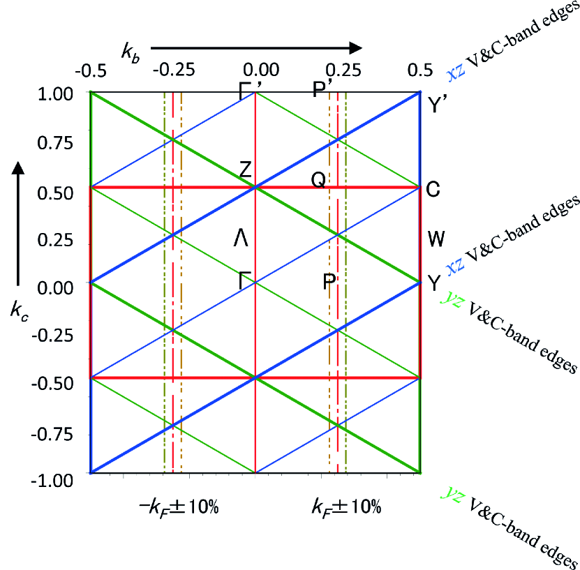
Figure 11: Double zone, same as FIG. 8 in Paper I. The $\genfrac{}{}{0.0pt}{}{1\mathrm{st}}{2\mathrm{nd}}$ physical zones shown in solid lines for the $xy$ (red), $xz$ (blue), and $yz$ (green) pure bands are respectively: $\left|k_{c}\right|\lessgtr\frac{1}{2}$, $\left|k_{c}+k_{b}\right|\lessgtr\frac{1}{2},$ and $\left|k_{c}-k_{b}\right|\lessgtr\frac{1}{2}.$ The red zone is the BZ, and its irreducible part is the one with $0\leq k_{c}\leq 0.5.$ Weak lines indicate the positions of pure-band maxima and minima (see FIG. I 6). The red dot-dashed lines indicate the positions of the left and the right doubly degenerate Fermi-surface sheets for stochiometric 2(LiMo₆O₁₇). The brown and olive dot-dashed lines respectively correspond to 10% hole and electron doping. See Sect. I IV.1.4 and Sect. X.4. The figure is to scale because the triangles are almost equilateral.

IX Theory of ARPES intensity variations in LiPB

Our ARPES data to be presented in Sect. X show (fine-grained) intensity variations between equivalent zones, similar to the BZ-selection effects observed in graphite and explained by Shirley et al. [68]. The primitive cell of LiPB, Li₂Mo₁₂O${}_{34},$ is however much larger than that of graphite, C${}_{2},$ and its ARPES intensity exhibits not only fine-grained zone selection, but also coarse-grained structures in reciprocal space. On the other hand, like in graphite, there are only four occupied bands in LiPB, and this together with the reduction of the dimensionality from 2D to quasi-1D enables a simple description for LiPB in terms of WOs. As we shall explain, it is the tails of the Mo1 and MO1-centered $t_{2g}$ WOs, $w_{m}\left(\mathbf{r}\right)$ and $W_{m}\left(\mathbf{r}\right)$ seen in FIG. I 9, which give rise to the coarse-grained structure, and it is the approximate equivalence I (17) by half a lattice translation which gives rise to the fine-grained structure. This zone-selection effect is simpler than the one found for the $\pi$-band in graphite because it is due to the existence of a hypothetical, un-dimerized form [LiMo₆O₁₇ in Charts I (21) and (22)] of LiPB, which cannot exist for C₂ where the two carbons are far from being separated by half a lattice vector.

IX.1 Preliminaries

We shall first follow the treatment of Shirley et al. [68], but in the next subsection switch from their representation of the initial-states in terms of atomic orbitals (AOs) to one in terms of WOs. Hence, we start from the one-step (Fermi’s golden rule) expression:

$$I\left(\mathbf{\kappa},\omega\right)\, \propto \,\theta\left(\omega\right)\sum\nolimits_{j\mathbf{k}}^{\mathrm{zone}}\delta\left[E_{j}\left(\mathbf{k}\right)+\omega\right]$$

$$\times\left|\left\langle e^{2\pi i\mathbf{{\kappa}\cdot r}}\left|\mathbf{p}\cdot\mathbf{E}\right|\psi_{j}\left(\mathbf{k,r}\right)\right\rangle\right|^{2},$$

for the photoemission intensity as functions of the electrons binding energy $\omega$ and momentum $\left(2\pi\right)\mathbf{\kappa}$ inside the sample. Surface effects are neglected. We have used the one-electron approximation with initial-state Bloch functions $\psi_{j}\left(\mathbf{k,r}\right)$ and energy bands $E_{j}\left(\mathbf{k}\right)$ with respect to the Fermi level. The sum in (IX.1) is over all occupied states $j\mathbf{k}$ with $\mathbf{k}$ in a (single) zone and $\sum\nolimits_{\mathbf{k}}$ denoting the average over this zone. For simplicity –and lack of knowledge– the final state inside the sample is taken as the plane wave $e^{2\pi i\mathbf{\kappa}\cdot\mathbf{r}},$ the least specific choice possible. For our purpose, it suffices to express the matrix element as:

$$\left\langle e^{2\pi i{\mathbf{\kappa}}\mathbf{\cdot r}}\left|\mathbf{p}\cdot\mathbf{E}\right|\psi_{j}\left(\mathbf{k,r}\right)\right\rangle\propto\left(\mathbf{\kappa\cdot\hat{e}}\right)\,\left\langle e^{2\pi i{\mathbf{\kappa}}\mathbf{\cdot r}}|\psi_{j}\left(\mathbf{k,r}\right)\right\rangle$$ (71)

as obtained by, first of all, operating with the dipole operator $\mathbf{p\cdot E}$ to the left, that is on the plane wave, and then by pulling the polarization-dependent factor from Eq. (100) outside the integral, exploiting the fact that the photon wavelength is long compared with inter-atomic distances. The proportionality constants in (IX.1) and (71) are independent of the initial states.

Hence, photoemission at energy $\omega$ occurs for $\mathbf{\kappa}$ at the constant-energy contours $\omega=-E_{j}\left(\mathbf{\kappa}\left[\mathop{\mathrm{m}od}\mathrm{zone}\right]\right)$ with an intensity which, contrary to $E_{j}\left(\mathbf{k}\right),$ is aperiodic in the reciprocal lattice and depends on the polarization of the photons and on the initial states, $\psi_{j}\left(\mathbf{k,r}\right),$ of the electrons.

The initial states may be expanded in Bloch sums I (8) of localized orbitals $\chi_{RL}\left(\mathbf{r}\right)\mathbf{,}$ e.g. AOs, NMTOs, or WOs$:$

$$\psi_{j}\left(\mathbf{k,r}\right)=\sum\nolimits_{RL}^{\mathrm{cell}}\chi_{RL}\left(\mathbf{k,r}\right)\,u_{RL,j}\left(\mathbf{k}\right)=$$

$$\sum\nolimits_{RL}^{\mathrm{cell}}\sum\nolimits_{\mathbf{T}}\chi_{RL}\left(\mathbf{r-T}\right)e^{2\pi i\mathbf{k\cdot T}}u_{RL,j}\left(\mathbf{k}\right).$$ (72)

Since for a Bloch sum I (8) of orbitals, $\chi_{R}\left(\mathbf{r}\right)$ centered${}^{\text{I}\,\ref{Rcenter}}$ at $\mathbf{r\mathrm{=}R}$,

$$\left\langle e^{2\pi i\mathbf{{\kappa}\cdot r}}|\chi_{R}\left(\mathbf{k,r}\right)\right\rangle=$$ (73)

$$e^{-2\pi i\mathbf{{\kappa}\cdot R}}\int\chi_{R}\left(\mathbf{r}\right)e^{-2\pi i\mathbf{{\kappa}\cdot}\left(\mathbf{r-R}\right)}d^{3}r\sum_{\mathbf{T}}e^{-2\pi i\left(\mathbf{{\kappa}-k}\right)\mathbf{\cdot T}}$$

$$= e^{-2\pi i\mathbf{{\kappa}\cdot R}}\tilde{\chi}_{R}\left(\mathbf{\kappa}\right)\sum\nolimits_{\mathbf{G}}\delta\left(\mathbf{\kappa}-\mathbf{k}-\mathbf{G}\right),$$

where the sum is over all points, G, of the reciprocal lattice and

$$\tilde{\chi}_{R}\left(\mathbf{\kappa}\right)\equiv\int\chi_{R}\left(\mathbf{r}\right)e^{-2\pi i\mathbf{{\kappa}\cdot}\left(\mathbf{r-R}\right)}d^{3}r$$ (74)

is the Fourier transform (FT) of $\chi_{R}\left(\mathbf{r}\right).$ Note that we use a notation according to which real-space functions such as $\chi_{R}\left(\mathbf{r}\right)$ are centered at $r$=$R$, but their Fourier transforms, $\tilde{\chi}_{R}\left(\mathbf{\kappa}\right)$ defined by (74), only depend on their shape and not on where they are centered.

The second factor of the matrix element (71) thus factorizes as:

$$\left\langle e^{2\pi i\mathbf{{\kappa}\cdot r}}|\psi_{j}\left(\mathbf{k,r}\right)\right\rangle = \sum\nolimits_{RL}^{\mathrm{cell}}e^{-2\pi i\mathbf{{\kappa}\cdot R}}\tilde{\chi}_{RL}\left(\mathbf{\kappa}\right)u_{RL,j}\left(\mathbf{k}\right)$$

$$\times\sum\nolimits_{\mathbf{G}}\delta\left(\mathbf{\kappa}-\mathbf{k}-\mathbf{G}\right),$$

whereby expression (IX.1) for the photoemission intensity becomes:

$$I\left(\mathbf{\kappa},\omega\right)\propto\left(\mathbf{{\kappa}\cdot\hat{e}}\right)^{2}\theta\left(\omega\right)\sum_{j\mathbf{k}}^{\mathrm{zone}}\delta\left[E_{j}\left(\mathbf{k}\right)+\omega\right]\times$$ (75)

$$\left|\sum_{RL}^{\mathrm{cell}}e^{-2\pi i\mathbf{{\kappa}\cdot R}}\tilde{\chi}_{RL}\left(\mathbf{\kappa}\right)u_{RL,j}\left(\mathbf{k}\right)\sum_{\mathbf{G}}\delta\left(\mathbf{\kappa}-\mathbf{k}-\mathbf{G}\right)\right|^{2},$$

which vanishes unless the wave-vector, $\mathbf{\kappa,}$ of the final electronic state inside the sample (see Sect. X.1) equals the Bloch vector, $\mathbf{k,}$ of the initial electronic state, plus an arbitrary reciprocal lattice vector, $\mathbf{G}$. In (75), $\sum_{\mathbf{G}}$ is a periodic function of $\mathbf{\kappa-k}$ in the $\mathbf{G}$-lattice, but the other factors are not.

An AO factorizes as: $\chi_{RL}\left(\mathbf{r}\right)\equiv Y_{L}\left(\widehat{\mathbf{r}_{R}}\right)\varphi_{Rl}\left(r_{R}\right),$ whereby its FT (74), which depends on its shape, $L,$ including its orientation, but not on its center, $\mathbf{R,}$ can be taken outside the sum over translationally equivalent AOs:

$$\sum_{R\in\mathrm{eq}}^{\mathrm{cell}}e^{-2\pi i\mathbf{{\kappa}\cdot R}}\tilde{\chi}_{RL}\left(\mathbf{\kappa}\right)u_{RL,j}\left(\mathbf{k}\right)=$$ (76)

$$\tilde{Y}_{L}\left(\mathbf{\hat{\kappa}}\right)\int j_{l}\left(2\pi\kappa r\right)\varphi_{Rl}\left(r\right)r^{2}dr\sum_{R\in\mathrm{eq}}^{\mathrm{cell}}e^{-2\pi i\mathbf{k}\cdot\mathbf{R}}u_{RL,j}\left(\mathbf{k}\right),$$

thus leaving the sums $\mathop{\textstyle\sum}_{R\notin\mathrm{eq}\,L}^{\mathrm{cell}}$ over the translationally inequivalent AOs to be performed later. Hence, the sum (76) over translationally equivalent AOs factorizes into a $\mathbf{\kappa}$-dependent AO form factor, times a so-called (Ref. 70, 71, 72) photoemission structure factor (PSF). The latter is similar to the geometrical structure factor in x-ray diffraction, but depends on the initial-state wave function [via its LCAO coefficients, $u_{RL,j}\left(\mathbf{k}\right)$]. This factorization holds for the $\pi$-band in C₂, because this band is singly degenerate and contains only one type of orbital, $Y_{10}\mathrm{=}p_{z},$ so that the entire sum, $\sum_{RL}^{\mathrm{cell}}e^{-2\pi i\mathbf{{\kappa}\cdot R}}\tilde{\chi}_{RL}\left(\mathbf{\kappa}\right)u_{RL,j}\left(\mathbf{k}\right),$ reduces to the factorized form (76). The PSF for the graphene $\pi$-band thus depends merely on the $\mathbf{k}$-dependent phase between the $p_{z}$ orbitals on the two atoms [68]. However, to the three $\sigma$-bands in graphene three translationally inequivalent AOs on each of the two C atoms ($s,$ $p_{x},$ and $p_{y},$ or the three equivalent $sp^{2}$ orbitals directed towards the three nearest neighbors) contribute, so that for the $\sigma$-bands, $\sum_{RL}^{\mathrm{cell}}e^{-2\pi i\mathbf{{\kappa}\cdot R}}\tilde{\chi}_{RL}\left(\mathbf{\kappa}\right)u_{RL,j}\left(\mathbf{k}\right)$ does not factorize into an orbital form factor and a geometrical structure factor.

Whereas 8 AOs are needed to describe the occupied bands in graphene, LiPB needs more than 300 atomically localized AOs (see Sect. I II), but -by virtue of its quasi-1D structure- merely the six $t_{2g}$ WOs shown in FIG. I 9. Using those in expression (75) for the ARPES intensity and neglecting inter-$m$ mixing, leads to great simplification, as we shall now see:

IX.2 Using the six $t_{2g}$ WOs

For LiPB, we shall predict, and in Sect. X.5 confirm, that the near-translational equivalence of the $t_{2g}$ WOs, $w_{m}\left(\mathbf{r}\right)$ and $W_{m}\left(\mathbf{r}\right),$ by half a lattice translation causes the ARPES to have double-period fine-grained intensity variations which approximately follow the $\left|\mathbf{k}\right\rangle$ character I (63) shown in FIG.s I 6, 7, and 10 of the occupied bands. This implies that the $m$-band with the lower energy appears in the 1st- and is extinguished near the centre of the 2nd physical zone, and conversely for the $m$-band with the higher energy. On top of this, comes that the upper $xz$- and $yz$-bands are unoccupied and therefore cause no intensity in their respective 2nd physical zones. The metallic $xy$-band with the lower energy should best be seen in the 1st- and the $xy$-band with the higher energy in the 2nd BZ. This zone-selection effect will allow us to resolve the perpendicular dispersion and splitting of the quasi-1D $\widetilde{xy}$-bands predicted in the bottom panel of FIG. 14. We shall see that the deviations from the translational equivalence of $w_{m}\left(\mathbf{r}\right)$ and $W_{m}\left(\mathbf{r}\right)$, i.e. the inversion- and displacement dimerizations I (18), will distort the ARPES intensity variation from that of the initial-state $\left|\mathbf{k}\right\rangle$ character, $\frac{1}{2}\left[1\mp\cos\phi\left(\mathbf{k}\right)\right],$ to $\frac{1}{2}\left[1\mp\cos\left\{\phi\left(\mathbf{k}\right)-\eta\left(\mathbf{\kappa}\right)\right\}\right]$ where $\eta\left(\mathbf{\kappa}\right)$ is the dimerization phase shift of the emitted electron with momentum $\mathbf{\kappa}$. By suitable choice of $\kappa_{a},$ via control of the photon energy [see e.g. Eq. (104)], this distortion can be negligible for the $xy$-bands in a large part of the double zone, and may also be so for the occupied $xz$ and $yz$ bands.

In addition to the fine-grained zone-selection effect (Sect. IX.2.1), well-known from the geometrical structure factor in x-ray crystallography, we shall predict (Sect. IX.2.2) and find (Sect. X) that the internal structure of the $w_{m}\left(\mathbf{r}\right)$ $t_{2g}$ WO, spreading out to about the four nearest molybdenums in its plane (see FIG. I 5), makes the form factor of the WO approximately factorize into a coarse-grained structure factor, times the form factor of the local partial-wave projection, $Y_{2m}\left(\mathbf{\hat{r}}\right)\varphi_{2}\left(r\right),$ of the WO tail.

IX.2.1 Zone selection; the fine-grained structure

The DFT calculation resulting in the low-energy six-band $t_{2g}$ TB Hamiltonian and in the band structures in FIG.s 20 (b) and 22 shows that –except near band crossings such as those below $-0.5$ eV and the ones near the top of the valence bands near Z– each band is dominated by one $m$ character. For describing the ARPES matrix elements, but not the bands, we shall neglect by-mixing of WOs with other $m$-values, i.e. use the pure-$m$ approximation (Sect. I VI.3). Therefore, in the general expression (72) for the the initial-state wave function, $L$ takes one value $\left(m\right),$ $R$ takes two values (Mo1 and MO1), and expression (72) becomes Eq. I (58) which is repeated in the Introduction to the present paper.

Hence, the second factor of the matrix element (71) for photoemission from the upper ($j$=2) or lower ($j$=1) $m$-band state is the FT of the respective eigenfunction I (58):

$$\left\langle e^{2\pi i\mathbf{{\kappa}\cdot r}}|w_{\genfrac{}{}{0.0pt}{}{2}{1}}\left(\mathbf{k,r}\right)\right\rangle = \frac{1}{\sqrt{2}}\sum_{\mathbf{G}}\delta\left(\mathbf{\kappa}-\mathbf{k}-\mathbf{G}\right)\left[\tilde{w}\left(\mathbf{\kappa}\right)e^{-i\phi\left(\mathbf{k}\right)}\mp\tilde{W}\left(\mathbf{\kappa}\right)e^{2\pi i\mathbf{\kappa\cdot d}}\right]$$ (77)

$$= \frac{1}{\sqrt{2}}\sum_{\mathbf{G}}\delta\left(\mathbf{\kappa-k-G}\right)\tilde{w}\left(\mathbf{\kappa}\right)\left[e^{-i\phi\left(\mathbf{k}\right)}\mp e^{-i\eta\left(\mathbf{\kappa}\right)}\right].$$

For the FTs of $w(\mathbf{k,r})$ and $W(\mathbf{k,r})$ we have used Eq. (73$)$ with the sum being over all points $\mathbf{G}$ of the reciprocal lattice. Inside this sum, the product of the phase factors, $e^{\pi i\left(k_{c}+k_{b}\right)}$ and $e^{-2\pi i\mathbf{\kappa\cdot}\left(\frac{\mathbf{c+b}}{2}-\mathbf{d}\right)},$ from respectively Eq.s I$~{}($58$)$ and (73$),$ is simply $e^{2\pi i\mathbf{\kappa\cdot d}}$ with $\mathbf{d}$ being the displacement dimerization I (16) and $\mathbf{\kappa}$ the momentum of the emitted electron. On the second line of Eq. (77) we have used that, due to the inversion dimerization I (18), $\tilde{W}\left(\mathbf{\kappa}\right)=$ $\tilde{w}\left(-\mathbf{\kappa}\right)$ and that $\tilde{w}\left(-\mathbf{\kappa}\right)=$ $\tilde{w}\left(\mathbf{\kappa}\right)^{\ast}=$ $\left|\tilde{w}\left(\mathbf{\kappa}\right)\right|e^{-i\arg\tilde{w}\left(\mathbf{\kappa}\right)}$ because $w\left(\mathbf{r}\right)$ is a real-valued $t_{2g}$ function. As a consequence, $e^{2\pi i\mathbf{\kappa\cdot d}}\tilde{W}\left(\mathbf{\kappa}\right)/\tilde{w}\left(\mathbf{\kappa}\right)=e^{-i\eta\left(\mathbf{\kappa}\right)},$ where

$$\eta_{m}\left(\mathbf{\kappa}\right)\equiv 2\arg\tilde{w}_{m}\left(\mathbf{\kappa}\right)-2\pi\mathbf{\kappa\cdot d},$$ (78)

is the dimerization phase shift whose first term is due to the inversion- and the second to the displacement dimerization. The latter, $2\pi\left(0.012\kappa_{a}+0.033\kappa_{c}\right)$ Eq. I (16), is a weak function of $\kappa_{c},$ a very weak function of $\kappa_{a},$ and independent of $\kappa_{b}$ and $m$. It is the dotted, linear curves shown in the first columns of FIG.s 12 and 13. The first term in expression (78), the phase shift due to inversion dimerization, is the dashed curves in the first columns which we have evaluated as will be explained in the next subsection IX.2.2 using the rough digitalizations (85) and (90) of FIG.s I 5 and I 9.

The intensity (75) of photoemission from two dimerized $m$-bands $\left(j\text{=}1,2\right)$ in LiPB is thus:

$$I\left(\mathbf{\kappa},\omega\right) \propto \left(\mathbf{{\kappa}\cdot\hat{e}}\right)^{2}\theta\left(\omega\right)\mathop{\displaystyle\sum}\limits_{j=1}^{2}\mathop{\displaystyle\sum}\limits_{\mathbf{k}}^{\mathrm{zone}}\delta\left[E_{j}\left(\mathbf{k}\right)-E_{F}+\omega\right]\left|\sum_{\mathbf{G}}\delta\left(\mathbf{\kappa}-\mathbf{k}-\mathbf{G}\right)\tilde{w}\left(\mathbf{\kappa}\right)\left[e^{-i\phi\left(\mathbf{k}\right)}\mp e^{-i\eta\left(\mathbf{\kappa}\right)}\right]\right|^{2}\propto$$ (79)

$$\sim \left(\mathbf{{\kappa}\cdot\hat{e}}\right)^{2}\left|\tilde{w}\left(\mathbf{\kappa}\right)\right|^{2}\theta\left(\omega\right)\mathop{\displaystyle\sum}\limits_{j=1}^{2}\mathop{\displaystyle\sum}\limits_{\mathbf{k}}^{\mathrm{zone}}\delta\left[E_{j}\left(\mathbf{k}\right)-E_{F}+\omega\right]\,\delta\left[\mathbf{\kappa}-\left(6,0,0\right)-\mathbf{k}\right]\,\frac{1\mp\cos\left[\phi\left(\mathbf{k}\right)-\eta\left(\mathbf{\kappa}\right)\right]}{2},$$

where the second line holds when –hinging on the coarse-grained structure of $\tilde{w}\left(\mathbf{\kappa}\right)$ and the experimental set up$-$ the $\mathbf{G}$-sum is dominated by one term, the one for $\mathbf{G}=\left(6,0,0\right)$ in our case, as we shall see in the following section, FIG.s 15 and 16 in particular. We can then use that $\frac{1}{4}\left|e^{-i\phi}\mp e^{-i\eta}\right|^{2}=$ $\left[1\mp\cos\left(\phi-\eta\right)\right]/2,$ which is like in Eq. I$~{}($63) and illustrated in FIG. I 10, but shifted by $\eta,$ and obtain the simple result that the intensity of photoemission from two dimerized $m$-bands $\left(j\text{=}1,2\right)$ in LiPB follows the $\left|\mathbf{k}\right\rangle$ character (fatness), but with the band-structure phase, $\phi\left(k_{b},k_{c}\right)$ [Eq. I (60) in the Introduction] shifted by the dimerization phase shift, $\eta\left(k_{a}+6,k_{b},k_{c}\right).$ Remembering that $\phi$ is independent of $k_{a}$ due to the long paths for hopping between slabs${}^{\text{I}\,\text{\ref{slabhop}}}$ and varies from –$\frac{\pi}{2}$ to $+\frac{\pi}{2}$ across the 1st zone, we realize that dimerization phase shift shown by the full curves in the first columns of FIG.s 12 and 13 can merely distort the switching curves, and less so for the $xy$-bands than for the equivalent $yz$- and $xz$-bands. This is seen in the middle panels of FIG.s 12 and 13. For the $xy$-bands along the $\kappa_{b}$=$0.225$ line slightly inside the FS the distortions increase with the deviation of $\kappa_{a}$ from the value $6.8.$ Similarly for switching curves for the $yz$-bands, also along the $\kappa_{b}$=$0.225$ line, in FIG. 13 the distortions increase with the deviation of $\kappa_{a}$ from the value $5.3.$

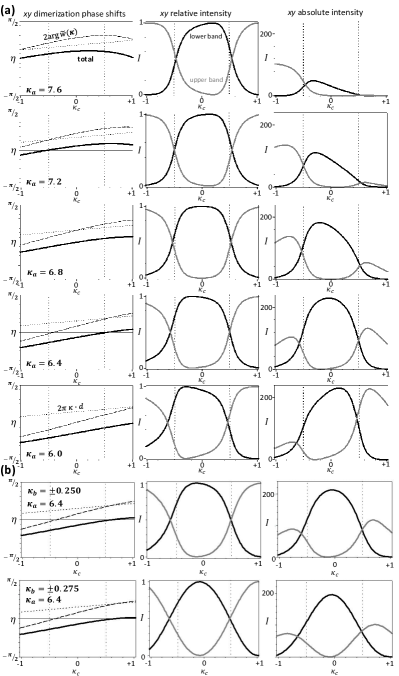
Figure 12: (a) Photoemission from the $xy$-bands (red in FIG. 14) for $\left|\kappa_{b}\right|$=$\left|k_{b}\right|=0.225$ and as functions of $\kappa_{c}$=$k_{c}$ in the double zone, i.e. along a brown dot-dashed line in FIG. 11. See also FIG. I 10. Column 1: Inversion- ($2\arg\tilde{w}\left(\mathbf{\kappa}\right),$ dash), displacement- ($2\pi\mathbf{\kappa\cdot d,}$ dots), and total ($\eta\left(\mathbf{\kappa}\right),$ full) dimerization phase shift for $\kappa_{a}=6.0-7.6$. Column 2: Relative intensities of photoemission, $\left[1\mp\cos\left\{\phi\left(\mathbf{k}\right)-\eta\left(\mathbf{\kappa}\right)\right\}\right]/2,$ from the upper (light) and lower (dark) bands. These intensities exhibit the fine-grained structure. Column 3: Absolute photoemission intensities, i.e. the relative intensities in column 2, times the polarization- and WO form factors, $\left(\mathbf{{\kappa}\cdot\hat{e}}\right)^{2}\left|\tilde{w}\left(\mathbf{\kappa}\right)\right|^{2},$ evaluated in Sect. IX.2.2 and shown in the top panel of FIG. 14. These polarization- and WO form factors provide the coarse-grained structure. (b) same as (a), but along $\left|\kappa_{b}\right|$=$\left|k_{b}\right|=0.250,$ a red dot-dashed line in FIG. 1 (top), and along $\left|\kappa_{b}\right|$=$\left|k_{b}\right|=0.275,$ an olive dot-dashed line (bottom), and only for $\kappa_{a}=6.4.$ The boundaries of the 1st zone are indicated by vertical, dotted lines.

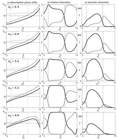
Figure 13: Same as in FIG. 12, but for the $yz$ bands (green in FIG. 14) and for $\kappa_{a}=4.8-6.4.$ The green zone boundaries in FIG. 11 intersect the brown dot-dashed near-FS line, $\kappa_{b}$=$0.225,$ at $\kappa_{c}$=$0.275$ and at $0.275-1=\allowbreak-0.725,$ which is where the swiching curves would have crossed, had there been no dimerization distortion, i.e. if $\eta_{yz}\left(\mathbf{\kappa}\right)$=0. Since the upper $yz$ band is empty, the light switching curves should have been deleted.

As seen in the 1st columns of FIG.s 12 and 13, the inversion (dash) and displacement (dots) phase shifts tend to cancel out: For the $xy$-bands along $\kappa_{b}$=$0.225$, a zero of $\eta\left(\mathbf{\kappa}\right)$ (full) increases through the 1st $xy$-zone ($-\frac{1}{2}|\frac{1}{2})$ for $\kappa_{a}$ decreasing from 7.4 to 6.4, and for the $yz$-bands along the same line, the zero decreases through the 1st $yz$-zone for $\kappa_{a}$ decreasing from 5.5 to 4.5. In these intervals of $\kappa_{a},$ the $c$-axis dimerization hardly distorts the zone selection as seen in the 2nd column. That the distortions due to displacement and inversion dimerizations tend to cancel over a $\kappa_{a}$ region of order 1 for both the $xy$- and $yz$-bands is surprising considering the fact that the $dd\delta$ coupling between the $xy\left(\mathbf{r}\right)$ and $XY\left(\mathbf{r-}\frac{\mathbf{c+b}}{2}+\mathbf{d}\right)$ WOs, is much smaller $dd\pi$ coupling between $yz\left(\mathbf{r}\right)$ and $YZ\left(\mathbf{r-}\frac{\mathbf{c+b}}{2}+\mathbf{d}\right),$ but for the latter the distortions are of course larger.

As mentioned already in connection with FIG. I 10, the $xy$ switching curves are even functions of $\kappa_{b}$ whose sharpness decreases with increasing $\left|\kappa_{b}\right|$. That this holds, also when dimerization distortion is included, may be seen from FIG. 12 for $\kappa_{a}$=6.4 by comparison of the switching curves for $\kappa_{b}$=0.225, 0.250 and 0.275.

In Sects. X.2 and X.3 we shall explain how $\kappa_{a}$ is deduced and how it is controlled by the photon energy, $h\nu$. From all FIG.s 12-18, we thus conclude that with proper $m$-dependent choice of the photon energy, the selection rule works well for each of the three $\left\{\mathbf{k,k+c}^{\ast}\right\}$-pairs of quasi-1D $t_{2g}$-bands in LiPB.

Figure 14: Top: Polarization- and form factor intensities, $\left(\mathbf{{\kappa}\cdot\hat{e}}\right)^{2}\left|\tilde{w}_{m}\left(\mathbf{\kappa}\right)\right|^{2}$, for $m$=$xy$ red, $xz$ blue, and $yz$ green along the P’QPQP’ line, $\kappa_{b}$=0.225, in the double zone $-1<\kappa_{c}\leq 1.$ These aperiodic, coarse-grained intensities depend on $\kappa_{a}$ –chosen here to be 6.4– as explained in Sect. X.2. Middle and bottom: Band-factor intensities according to Eq. (79) without dimerization, i.e. with $\eta_{m}\left(\mathbf{\kappa}\right)=0.$ They are the $\left|\mathbf{k}\right\rangle$-projected bands [see Eq. I (63)] and give rise to the fine-grained intensity distributions with period 2 in $\kappa_{c}.$ Their dependence on $\kappa_{a}$ is negligible. Like in FIG.s I 6 and I 7 the red $xy$ bands in the middle are pure, while the dark-red $\widetilde{xy}$ bands at the bottom are perturbed by the $xz$ and $yz$ valence and conduction bands. The $\left(\mathbf{k,k+c}^{\ast}\right)$-hybridization of the $\widetilde{xy}$-bands is seen to effectively extend over a $k_{c}$-region of width 0.3 around the BZ boundaries, $k_{c}=\frac{1}{2}+\mathop{\mathrm{i}nteger}.$ The zero of energy is the center of the gap in the $xz$ and $yz$ bands, whereby $E_{F}$=75 meV (see Sect. I VI). The occupation factor, $\theta\left(\omega\right)$ in Eq. (79), will remove the intensity from the bands with $E>E_{F}$.

In Paper III, we shall study the dispersion of the two quasi-1D bands in the gap and –as demonstrated by comparison of the red and dark-red bands in respectively the middle and bottom parts of FIG. 14– this requires that we take the weak hybridization of these $xy$-like bands with the $xz$ and $yz$ valence and conduction bands into account. This we shall do by downfolding those characters into the tails of the $xy$ WOs, which thereby attain longer range and become what we call $\widetilde{xy}$ WOs. The concomitant modification of the WO form factor –and, hence, dimerization phase shift– we shall neglect. What the weak hybridization primarily changes is the dispersion of the $\widetilde{xy}$ energy-bands. As mentioned before, a main goal of the present and the following Paper III is to detect with ARPES the predicted dispersion in the perpendicular $\left(k_{c}\right)$ direction, most noticeably the resonance peaks in the upper $\widetilde{xy}$-band caused by the weak hybridization with the $yz$- and $xz$-bands and expected to be seen near respectively $\kappa_{c}$=$-0.75$ and 0.75. To see both the former resonance peak and its cause, the lower $yz$-band, in the same ARPES experiment like in FIG. 14 is, however, impossible because the former requires using $\kappa_{a}\sim 7.2$ and the latter $\kappa_{a}\sim 4.5.$

The Brillouine-zone-dependent photoemission intensity derived and discussed here based on a structure and form factor should be generally applicable to different materials. The main approximation made is in Eq.(IX.1). We approximate the wave-function of the photo-emitted electron by a plane wave. The free electron state, should in principle be a Bloch wave with an additional modification due to the sample surface. The approximation can become noticeable if the k vector of the free electron is close to a zone boundary, where small periodic potentials are expected to gap degenerate free electron states. A full understanding of the importance of describing the state of the photo-electron beyond a plane wave and including surface effects can be investigated with multiple scattering techniques [73] but a simple intuitive picture is currently missing and should be further investigated. At the same time, calculations for graphene [68] or Bi₂Se₃ [74, 75] assuming the photo-electron to be a plane wave seem to capture a large part of the Brillouin zone dependent intensity and agree well with experiment.

IX.2.2 WO form factor, $\tilde{w}_{m}\left(\mathbf{\kappa}\right),$ inversion dimerization, and the coarse-grained structure

A $t_{2g}$ WO, $w_{m}\left(\mathbf{r}\right),$ has a halo with contributions (tails) on the near Mo neighbors in the plane of this flat WO with the same $m$ character as that of its head (see FIG.s 5 and 9 in Paper I). For the present purpose, we shall neglect the hybridization between WOs with different values of $m,$ as well as the details of the oxygens which $pd\pi$ anti-bond with the WO head and bond with the tail. What is important, is that the head has a partial-wave shape, $Y_{m}\left(\mathbf{\hat{r}}\right)\varphi_{2}\left(r\right),$ which is translated to the Mo$\,n$ neighbors and multiplied by a factor, $c_{n}$$<$1. This makes the FT, $\tilde{w}_{m}\left(\mathbf{\kappa}\right),$ of the WO factorize approximately into an orbital-dependent structure factor, $\mathcal{S}_{m}\left(\mathbf{\kappa}\right),$ times the FT of $Y_{m}\left(\mathbf{\hat{r}}\right)\varphi_{2}\left(r\right):$

$$\tilde{w}_{m}\left(\mathbf{\kappa}\right)\propto\mathcal{S}_{m}\left(\mathbf{\kappa}\right)\tilde{Y}_{m}\left(\mathbf{{\hat{\kappa}}}\right)\int_{0}^{0.55}j_{2}\left(2\pi\kappa r\right)\varphi_{\mathrm{Mo}\,d}\left(r\right)r^{2}dr.$$ (80)

We have not computed the form factor by accurate, numerical FT of the WO, but shall use the factorization (80) together with the real-space figures to provide a qualitative understanding of the ARPES data to be presented in the following section.

Whereas the radial and angular factors, $\int_{0}^{0.55}j_{2}\left(2\pi\kappa r\right)\varphi_{\mathrm{Mo}\,d}\left(r\right)r^{2}dr$ and $\tilde{Y}_{m}\left(\mathbf{{\hat{\kappa}}}\right),$ are even, real functions of $\mathbf{\kappa,}$ the structure factor, $\mathcal{S}_{m}\left(\mathbf{\kappa}\right),$ is a complex function whose real and imaginary parts, like those of $\tilde{w}_{m}\left(\mathbf{\kappa}\right),$ are respectively even and odd. From the WO figures I 5 and 9, we estimate these structure factors (the $c_{n}$ coefficients$)$ to be:

$$\mathcal{S}_{xy}\left(\mathbf{\kappa}\right) \sim \left[\begin{array}[]{ccc}&+\frac{1}{2}e^{2\pi i\kappa_{y}}&+\frac{1}{6}e^{2\pi i\left(\kappa_{x}+\kappa_{y}\right)}\\ +\frac{1}{4}e^{-2\pi i\kappa_{x}}&1&+\frac{1}{2}e^{2\pi i\kappa_{x}}\\ &+\frac{1}{4}e^{-2\pi i\kappa_{y}}&\end{array}\right]$$ (85)

$$\left/\left(1+\frac{1}{2}+\frac{1}{2}+\frac{1}{4}+\frac{1}{4}+\frac{1}{6}\right)\right.,$$

$$\mathcal{S}_{yz}\left(\mathbf{\kappa}\right) \sim \left[\begin{array}[]{ccc}+\frac{1}{8}e^{2\pi i\left(\kappa_{z}-\kappa_{y}\right)}&+1e^{2\pi i\kappa_{z}}&0\\ +\frac{1}{3}e^{-2\pi i\kappa_{y}}&1&+\frac{1}{2}e^{2\pi i\kappa_{y}}\\ 0&+\frac{1}{4}e^{-2\pi i\kappa_{z}}&0\end{array}\right]$$ (90)

$$\left/\left(1+1+\frac{1}{2}+\frac{1}{3}+\frac{1}{4}+\frac{1}{8}\right)\right.,$$

and $\mathcal{S}_{xz}\left[\kappa_{x},\kappa_{z}\right]$=$\mathcal{S}_{yz}\left[\kappa_{y},\kappa_{z}\right].$

In FIG. I 5 we clearly see that the inversion symmetry of the $xy$ WO around its center, Mo1, is far better preserved than that of the $yz$ WO. The inversion dimerization I (18) is $w_{m}\left(-\mathbf{r}\right)-w_{m}\left(\mathbf{r}\right),$ and the phase shift (78) due to inversion dimerization is $2\arg\tilde{w}\left(\mathbf{\kappa}\right)=2\arg S\left(\mathbf{\kappa}\right).$ The latter function is easily found from Eq. (85) for $xy$ and from (90) for $yz,$ and was used to produce FIG.s 12 and 13. Since $\mathcal{S}_{xz}\left[\kappa_{x},\kappa_{z}\right]$=$\mathcal{S}_{yz}\left[\kappa_{y},\kappa_{z}\right],$ we have: $\eta_{xz}\left[\kappa_{x},\kappa_{z}\right]$=$\eta_{yz}\left[\kappa_{y},\kappa_{z}\right].$

The structure factors, $\mathcal{S}_{xy},$ $\mathcal{S}_{yz},$ and $\mathcal{S}_{xz},$ peak –with value 1 if the normalizations are as above– along the respective lines: $\left[\kappa_{x},\kappa_{y},\kappa_{z}\right]$=$\left[\text{{l,m}},\kappa_{z}\right]$, =$\left[\kappa_{x},\text{{m,n}}\right]$, and =$\left[\text{{l,}}\kappa_{y},\text{{n}}\right],$ passing through the respective points, l$\mathbf{x}^{\ast}+$m$\mathbf{y}^{\ast}+$n$\mathbf{z}^{\ast},$ of the lattice reciprocal to the lattice I (12) with 1 Mo per primitive cell. In other words: $\left|\mathcal{S}_{xy}\right|^{2},$ $\left|\mathcal{S}_{yz}\right|^{2},$ and $\left|\mathcal{S}_{xz}\right|^{2}$ form 2D square lattices of ”beams” running in respectively the $\kappa_{z},$ $\kappa_{x},$ and $\kappa_{y}$ directions (see FIG. 15). This gives rise to intensity patterns that are coarser than the zone-selection patterns ($M+N$ even or odd) whose origin is the smallness of the dimerization that increases the size of the primitive cell from 6 to 12 molybdenums.

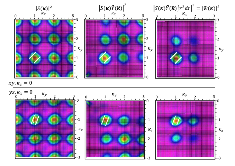
Figure 15: Form-factor intensities, $\left|\tilde{w}_{m}\left(\mathbf{\kappa}\right)\right|^{2},$ i.e. the coarse-grained structure. Top row: $xy$ form-factor intensities in the $\kappa_{z}$=0 plane. Bottom row: $yz$ form-factor intensities in the $\kappa_{x}$=0 plane. $\tilde{w}_{xz}\left(\kappa_{x},\kappa_{y},\kappa_{z}\right)$  =  $\tilde{w}_{yz}\left(\kappa_{y},\kappa_{x},\kappa_{z}\right).$ Columns 1-3: Turning on factors following Eq. (80) with $\mathcal{S}_{m}\left(\mathbf{\kappa}\right)$ given by Eq.s (85) and  (90).  The little white lines are the projections onto the $\kappa_{z}$=0 plane or the $\kappa_{x}$=0 plane of the near-FS lines $\left|\kappa_{b}\right|\sim\frac{1}{4},$ limited to the double zone $-1\leq\kappa_{c}\leq 1,$ along which the bands and fine-grained intensities for $\kappa_{a}$=6.4 were plotted in FIG. 14. The $\kappa_{a},$ $\kappa_{b},$ and $\kappa_{c}$ directions are those of respectively $\kappa_{x}+\kappa_{y}-\kappa_{z},$ $\kappa_{y}-\kappa_{x},$ and $\kappa_{x}+\kappa_{y}+2\kappa_{z};$ see Eq. (92).

The relation between the $\left[\kappa_{x},\kappa_{y},\kappa_{z}\right]$- and the $\left(\kappa_{a},\kappa_{b},\kappa_{c}\right)$-components –used to describe respectively the WO and the band structure and, hence, respectively the coarse and the fine-grained structure– is:

$$\genfrac{}{}{0.0pt}{}{\kappa_{x}}{\kappa_{y}}=\frac{\kappa_{a}+\kappa_{c}}{6}\mp\frac{\kappa_{b}}{2}\;\mathrm{and}\;-\kappa_{z}=\frac{\kappa_{a}+\kappa_{c}}{6}-\frac{\kappa_{c}}{2},$$ (91)

which is the same as the transformation I (12) between the primitive translations of the approximately cubic Mo₁- and the exact Mo₁₂-lattice [see also Charts I (14) and I (15)]. The inverse transformation –the same as I (13)– is:

$$\kappa_{a} = 2\left(\kappa_{x}+\kappa_{y}-\kappa_{z}\right),$$ (92)

$$\kappa_{b} = \kappa_{y}-\kappa_{x},\;\mathrm{and}\;\kappa_{c}=\kappa_{x}+\kappa_{y}+2\kappa_{z}.$$

Since exchange of $\kappa_{x}$ and $\kappa_{y}$ merely causes $\kappa_{b}$ to change sign, $\mathcal{S}_{xz}\left(\kappa_{a},\kappa_{b},\kappa_{c}\right)$ $=$ $\mathcal{S}_{yz}\left(\kappa_{a},-\kappa_{b},\kappa_{c}\right).$

The angular factors $\tilde{Y}_{m}\left({\mathbf{\kappa}}\right)$ in expression (80) have the same orientation with respect to the $a^{\ast}b^{\ast}c^{\ast}$ system as $Y_{m}\left(\mathbf{\hat{r}}\right)$ has with respect to the $abc$ system seen in FIG. I 5 and Charts I (14)-(15). This is so because the $abc$ system is (almost) orthogonal (Sect. I III), whereby $\mathbf{a}$ is parallel with $\mathbf{a}^{\ast},$ $\mathbf{b}$ with $\mathbf{b}^{\ast},$ and $\mathbf{c}$ with $\mathbf{c}^{\ast}.$ As a result:

$$\tilde{Y}_{xy}\propto-\frac{\kappa_{x}\kappa_{y}}{\kappa^{2}}=\left(\frac{\kappa_{b}}{2\kappa}\right)^{2}-\left(\frac{\kappa_{c}+\kappa_{a}}{6\kappa}\right)^{2},$$ (93)

where:

$$\kappa^{2}\equiv\kappa_{x}^{2}+\kappa_{y}^{2}+\kappa_{z}^{2}=\frac{1}{12}\kappa_{a}^{2}+\frac{1}{2}\kappa_{b}^{2}+\frac{1}{6}\kappa_{c}^{2},$$ (94)

and similarly for $\tilde{Y}_{yz}$ and $\tilde{Y}_{xz}.$ The angular factor extinguishes the intensity around the $\left[0,0,\kappa_{z}\right]$-, $\left[\kappa_{x},0,0\right]$-, or $\left[0,\kappa_{y},0\right]$-lines, as is clearly seen when proceeding from the 1st to the 2nd column in FIG. 15.

The last, radial factor in Eq. (80) is independent of $m$ and merely gives the overall shape of the ARPES intensity. We found it sufficient to mimic the main part of the Mo $4d$ radial function, continued for $r>0.5$ (in units of $3.82\mathrm{\mathring{A})}$ as the $t_{2g,m}$-average of the neighboring $pd\pi$ anti-bonds, by $\varphi_{2}\left(r\right)\propto\left(e^{-14r}-e^{-7}\right)r^{2}.$ This function peaks at $r\approx$0.14, has at node at 0.5, and is truncated at 0.55. The negative part mimics the contribution from the $pd\pi$ antibonds. The last factor in (80) thus raises quadratically from $\kappa$=0 and peaks at $\kappa\approx\sqrt{3},$ which is at the sphere passing through $\left[1,1,-1\right].$ For larger values of $\kappa$, the radial factor decreases monotonically and for $\kappa\gtrsim 3,$ i.e. outside the sphere passing through $\left[1,2,-2\right]$ and $\left[2,1,-2\right],$ it has fallen to below one third its value at the peak. The radial factor has been included in the two last columns of FIG. 15.

We thus realize that the angular and radial factors leave intensity in only small parts of reciprocal space.

The $xy$ form-factor intensity, $\left|\tilde{w}_{xy}\left(\mathbf{\kappa}\right)\right|^{2},$ shown in the 1st row and 3rd column in FIG. 15, has one dominant peak; its position is at $\left[\kappa_{x},\kappa_{y}\right]=\left(1+\frac{\epsilon}{6}\right)\left[1,1\right],$ where the small shift away from [1,1], proportional to $\epsilon\sim$0.4, is mainly due to the angular factor. In 3D, and according to Eq. (92), this peak becomes a beam centered on the line given by:

$$\kappa_{a}+\kappa_{c}=6+\epsilon\;\mathrm{and}\;\kappa_{b}=0.$$ (95)

This holds as long as the $\kappa_{z}$ dependence from the radial factor can be neglected. There are two, less intensive peaks near $\left[\kappa_{x},\kappa_{y}\right]$=$\left[1,2\right]$ and $\left[2,1\right],$ which in 3D become beams around the lines given by:

$$\kappa_{a}+\kappa_{c}=9\;\mathrm{and\;}\kappa_{b}=\pm 1.$$ (96)

In FIG. 16 we show the intensity distributions, $\kappa_{a}^{2}\left|\tilde{w}_{m}\left(\mathbf{\kappa}\right)\right|^{2},$ in the planes with $\kappa_{a}$=6.0 and 6.8 in the region $-0.5\leq\left(\kappa_{b},\kappa_{c}\right)\leq 1.5$. In the left-hand panel, we see the $xy$ beam (95) form spots around the points $\left(\kappa_{b},\kappa_{c}\right)=(0,\epsilon)$ and $(0,\epsilon-0.8)$ when hitting the $\kappa_{a}$=6.0 and 6.8 planes. In the latter plane, the less intensive spot centered near $\left(\kappa_{b},\kappa_{c}\right)$=$\left(1,2.2\right)$ and formed by the positive-$\kappa_{b}$ beam (96) can be barely seen.

The $yz$ form-factor intensity of zone selection, shown in the 2nd row and 3rd column in FIG. 15, has its dominant peak near $\left[\kappa_{y},\kappa_{z}\right]$=$\left[1,-1\right].$ In 3D, this peak becomes a beam centered on the line given by:

$$\kappa_{a}-2\kappa_{c}=6\;\mathrm{and}\;\kappa_{b}+\kappa_{c}=0.$$ (97)

There are two weaker peaks at $\left[\kappa_{y},\kappa_{z}\right]$=$\left[2,-1\right]$ and $\left[1,-2\right],$ which in 3D become beams centered along the lines given by respectively:

$$\kappa_{a}-2\kappa_{c}=6\;\mathrm{and\;}\kappa_{b}+\kappa_{c}=2,$$ (98)

and

$$\kappa_{a}-2\kappa_{c}=12\;\mathrm{and\;}\kappa_{b}+\kappa_{c}=-2$$ (99)

In the right-hand panel of FIG. 16 we see the $yz$ beam (97) form spots around $\left(\kappa_{b},\kappa_{c}\right)$=$(0,0)$ and $\left(-0.4,0.4\right)$ upon hitting the $\kappa_{a}$=6.0 and 6.8 planes, as well as the beam (98) hitting these two planes at respectively $\left(\kappa_{b},\kappa_{c}\right)$=$\left(2,0\right)$ and $\left(1.6,0.4\right).$

The vertical and diagonal black lines, periodically repeated, but limited to the regions where the intensity exceeds 40 in the units used in FIG. 14, indicate the CECs with binding energy 0.1 eV for $xy$ and 0.5 eV for $yz.$ The CECs will be discussed in the experimental section X.4.

Since the $xz$ form-factor intensity is related to the one shown for $yz$ in FIG. 16 by a sign change of $\kappa_{b},$ we can see that only for $\kappa_{a}\sim 6.4$ do the $zx$ and $yz$ intensities along e.g. the P’QPQP’ $\left(0.225,\kappa_{c}\right)$-line reach roughly the same maximum value. This is the maximum at $\sim$ 250 seen in the top part of FIG. 14 and in the 3rd column of FIG. 13.

Our ARPES measurements, to be presented and discussed in the following section, were mainly performed in the neighborhood of the point $\left[\kappa_{x},\kappa_{y},\kappa_{z}\right]=\left[1,1,-1\right]$ which is close to the peaks of all three form factors and which is the $\Gamma$ point $\left(\kappa_{a},\kappa_{b},\kappa_{c}\right)=\left(6,0,0\right)$. It may be noted that upon going from the 1st to the 2nd column in the 1st row of FIG. 15, the angular factor sharpens up the [1,1] peak of the $xy$ intensity. The traces of the two FS sheets, $\left|\kappa_{b}\right|$=$\frac{1}{4},$ on the $\kappa_{a}$=6.4 plane and bound between the $\kappa_{c}$=$\pm$1 planes are the little white lines in FIG. 15, when projected onto the $\kappa_{z}$=0 plane in the 1st row and onto the $\kappa_{x}$=0 plane in 2nd row. These are the P’QPQP’ lines along which the intensity distributions were shown in FIG. 14. Since the $xy$-band disperses in the direction of the $\kappa_{b}$-lobe of its WO, this direction is perpendicular to the little white lines.

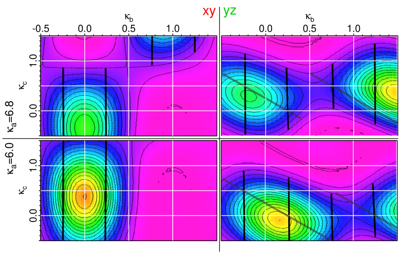
Figure 16: Theoretical $xy$ (left) and $yz$ (right) coarse-grained ARPES intensity distributions, $\kappa_{a}^{2}\left|\tilde{w}_{m}\left(\mathbf{\kappa}\right)\right|^{2},$ in the $\kappa_{b}\kappa_{c}$ planes with $\kappa_{a}$=6.0 (bottom) and 6.8 (top) planes. The $xz$ intensities equal the $yz$ ones mirrored around $\kappa_{b}$=0. See top part of FIG. 14 and Eq.s (79) and (95)-(99). The contours go from 0 to 400 in steps of 20. The black lines extending where the intensity exceeds 40 indicate $xy$ and $yz$ CECs with energy respectively 0.1 and 0.5 eV below the Fermi level (see FIG. 20) and in the periodic zone scheme.

At the end of this long section IX, we emphasize the following two points:

Whereas the $k_{a}$-dependence of the $\left|\mathbf{k}\right\rangle$-projected bands, i.e. of the fine-grained structure, is negligible compared with the $k_{b}$- and $k_{c}$-dependencies, the $\kappa_{a}$-dependence of the aperiodic form factors, $\left|\tilde{w}_{m}\left(\mathbf{\kappa}\right)\right|^{2},$ i.e. of the coarse-grained structure, is strong, as strong as the dependence on $\kappa_{c}$ for $xy,$ and half as strong for $yz/xz$; see Eq.s (95)-(97). This is due to the form factors being 2D, $\propto\kappa_{x}\kappa_{y},$ $\kappa_{y}\kappa_{z},$ or $\kappa_{x}\kappa_{z},$ and to the orientation of the $t_{2g}$ orbitals with respect to the crystallographic axes I (13).

Since the low-energy WOs in LiPB are relatively extended (covering several atoms), the radial part of the WO form factors make the beams narrow and thus cause the ARPES intensity to depend rather strongly on the photon energy $h\nu,$ as we shall see in Sect. X.3.

X Presentation and discussion of the ARPES data

From the basics of the electronic structure in Sect. I IV we expect the two $\widetilde{xy}$-bands crossing the Fermi level to have by far the largest dispersion with $k_{b}\mathbf{,}$ i.e. along the ribbon, weak dispersion with $k_{c},$ i.e. up and down the staircase, weak $k_{c}$-dependent splitting caused by direct inter-ribbon hopping and by hybridization with the gapped $xz$- and $yz$-bands, and essentially no dispersion with $k_{a}$ due to the lack of hopping between staircases. In the following, we want to demonstrate that this strong one-dimensionality is indeed confirmed by our ARPES experiment. We also pay attention to the aperiodic variations of the ARPES intensity between equivalent zones and compare them with the coarse-grained intensity variations predicted in the preceding Sect. IX.2.2. The fine-grained intensity variations (zone selection) predicted in Sect. IX.2.1 will be observed in Sects. X.4 and X.5 where, most importantly, we also compare the band dispersions in detail with those predicted by the LDA as parametrized by the $t_{2g}$ TB Hamiltonian (Sect. I VI).

Intensity variations and one-dimensionality are also features of the ARPES $yz$- and $xz$-bands, but of course not near the Fermi level where they are gapped. Moreover, their one-dimensionality is with $k_{c}+k_{b}$ or $k_{c}-k_{b},$ rather than with $k_{b}.$

X.1 ARPES method

We measured several samples for the conclusions presented in this work. The samples came from two different crystal growers and were all prepared by a temperature gradient flux growth technique [76]. In the text, we refer to two samples G (M. Greenblatt) and H (J. He) representing the variation detectable in our experiments.

Photoemission measurements were performed at the MERLIN endstation (BL 4.0.3) of the Advanced Light Source with a Scienta R4000 electron detector. The polarization was set to linear vertical, i.e. in FIG. 20 the vector of the electric field horizontal. The temperature was set to $T$=26 K for sample G and $T$=6 Kfor sample H and the samples were cleaved while attached to the cold manipulator at $p\approx 4\times 10^{-11}$torr . The overall energy resolution was set to around 16 meV at photon energy $h\nu$=30 eV going up to around 40 meV at $h\nu$=100 eV. At $h\nu$=30 eV, the momentum resolution in the b*-direction is 2% of $k_{Fb}$ at half-filling (i.e. at nominal Li₁ stoichiometry), i.e. 0.005. With the solid-state definition of reciprocal space [see Sect. I III below Eq. (11)], this is $0.006$ Å^-1. The polarization vector in sample coordinates is:

$$\frac{\mathbf{E}}{\left|\mathbf{E}\right|}=\left(\begin{array}[]{c}e_{a}\\ e_{b}\\ e_{c}\end{array}\right)=\left(\begin{array}[]{c}\sin(65^{\circ}-\phi)\cos\theta\\ \sin(65^{\circ}-\phi)\sin\theta\\ \cos(65^{\circ}-\phi)\end{array}\right).$$ (100)

Here, $\phi$ is the polar rotation, and the $\theta$ the tilt angle. In our measurements, $\left|\phi\right|\lesssim 5{{}^{\circ}}$ and $\left|\theta\right|\lesssim 5{{}^{\circ}}$ resulting overall in a strong component along the $\mathbf{a}$-axis, normal to the cleavage plane, a weak component along the $\mathbf{c}$-axis, and a very weak component along the $\mathbf{b}$-axis.

LiMo₆O₁₇ is susceptible to oxygen loss caused by intense ultraviolet light where the desorption is due to the Knotek-Feibelman mechanism including a core level excited resonant Auger decay [77]. It shares this behavior with, i.e. NaMo₆O₁₇[78], K_0.3MoO₃[32], or oxides like TiO₂[79] and SrTiO₃[80]. We were not able to prevent this damage by oxygen dosing, as i.e. possible for SrTiO₃[81]. The reason might be the existence of both, tetrahedral and octahedral coordinated molybdenums. A small oxygen loss causes a slight electron doping, but, as time progresses, the ARPES signal eventually blurs. In order to prevent the loss, one concept might be to keep the photon energy below that of the lowest energy core level resonance. However, often there is higher-order light that still causes a slow degradation (with the timescale in the hours instead of minutes) and therefore our concept is to use a large homogenous area and slightly alter the position of the beam spot when the sample degradation begins.

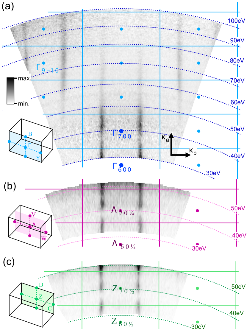
Figure 17: Photon energy scan of sample H at $T$=6 K for $\mathbf{\kappa}$ in three $\mathbf{a}^{\ast}\mathbf{b}^{\ast}$-planes: (a) FS map through $\kappa_{c}$=0 $\left(\mathrm{\Gamma BY}\right)$ (b) $\kappa_{c}$=$\frac{1}{4}$ $\left(\mathrm{\Lambda WV}\right)\mathrm{,}$ and (c) $\kappa_{c}$=$\frac{1}{2}$ $\left(\mathrm{ZDC}\right)\mathrm{.}$ The colored full lines along $\mathbf{a}^{\ast}$ and $\mathbf{b}^{\ast}$ are the intersections with the BZs. The blue dotted lines intersect at the reciprocal lattice points $\Gamma_{LMN}.$ The high-intensity traces represent the 1D FS showing no dispersion in the $\mathbf{a}^{\ast}$-direction. There are coarse-grained intensity variations whose origin is the structure factor of the form factor for the $xy$ WOs; see Sect. IX.2.2 and FIG. 18. This figure and the following are approximately to scale, i.e. consistent with $a/b=2.31.$

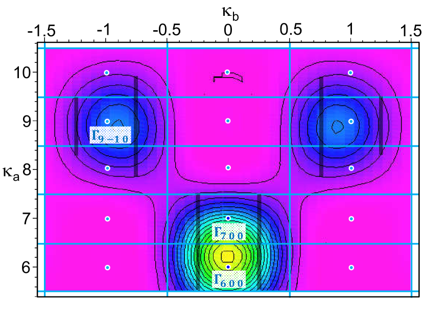
Figure 18: Theoretical ARPES intensity distribution $\kappa_{a}^{2}\left|\tilde{w}_{xy}\left(\kappa_{a},\kappa_{b},\kappa_{c}\text{=}0\right)\right|^{2}$ to be compared with the coarse-grained part of the experimental intensity distribution in FIG. 17. The contours go from 0 to 400 in steps of 20. The black lines indicate the traces of the near-FS sheets, $\left|\kappa_{b}\right|\sim\frac{1}{4}$, in the periodic zone scheme and extend where the intensity exceeds 40.

Even though the ARPES lineshapes have the general 1D holon-peak and spinon-edge features [3], they were analyzed by a model-free method described in detail in Paper III Sect. XV. This procedure was necessitated because the low-$T$ ARPES lineshape is not sharp enough to agree in detail with the low-$T$ TL lineshape [82]. If the TL lineshape is broadened ad hoc it can be made to fit [3], but we did not want to use that ad hoc procedure in the current work.

X.2 Ansatz for deducing $\kappa_{a}$

We repeat here some basics of ARPES, cf. [83, 84] As in Sect. IX.1 we use a notation according to which $\mathbf{k}$ denotes the Bloch vector in a (periodically repeated) single zone of an initial-state, and $\mathbf{\kappa}$ is the momentum of the final, plane-wave state inside the crystal. According to Eq. (79), $\mathbf{\kappa}\,\left[\mathop{\mathrm{m}od}\mathrm{zone}\right]=\mathbf{k.}$ Upon leaving the crystal, the photoelectron is diffracted in the direction away from the surface, whereby the normal momentum component, $\mathbf{\kappa}_{\perp}=\kappa_{a}\mathbf{a}^{\ast},$ jumps discontinuously to a smaller value, $\mathbf{\kappa}_{\perp o}.$ Parallel to the surface, the momentum is conserved:

$$\mathbf{\kappa}_{\mathbf{\shortparallel}}\equiv\kappa_{b}\mathbf{b}^{\ast}+\kappa_{c}\mathbf{c}^{\ast}=\mathbf{\kappa}_{\mathbf{\shortparallel}o}.$$

What is measured in ARPES is, for a given photon energy $h\nu,$ the yield, $I,$ the angle of exit, $\theta,$ and the kinetic energy, $T=\frac{h^{2}}{2m}\left|\mathbf{\kappa}_{o}\right|^{2},$ of the photoelectrons in the analyzer outside the crystal. The value of $\kappa_{a}$ inside the sample is deduced from the two latter quantities by assuming that inside the crystal, the energy of the final state is $V+\frac{h^{2}}{2m}\left|\mathbf{\kappa}\right|^{2},$ i.e. the energy of an electron, free with respect to a potential floor, $V,$ and that outside the crystal, the momentum is:

$$\mathbf{\kappa}_{o}=\left(\mathbf{\kappa}_{\perp o},\mathbf{\kappa}_{\shortparallel}\right)=\frac{\sqrt{2mT}}{h}\left(\cos\theta,\sin\theta\right),$$ (101)

and the energy is $\Phi+T.$ Here, $\Phi$ is the work function of the sample. It should not be confused with $\Delta\Phi$ which is a constant given by the apparatus and is essentially the difference between work function of sample and analyzer. $\Delta\Phi$ allows to relate the measured kinetic energy to the binding energy $\omega$ within the sample

$$\omega\equiv-E_{j}\left(\mathbf{k}\right)=h\nu-\left(\Delta\Phi+T\right).$$ (102)

Equating the inside and outside energies, yields the desired relation for $\kappa_{a}:$

$$\frac{\kappa_{a}}{a}=\left|\mathbf{\kappa}_{\perp}\right|=\frac{\sqrt{2m}}{h}\sqrt{T\cos^{2}\theta+V_{0}},$$ (103)

where $V_{0}\equiv\Phi-V$ is the so-called inner potential. Taking $V$ and $\Phi$ with respect to the Fermi level, which is common for the crystal and the analyzer, $V$ is negative and $\Phi$ is positive, whereby $V_{0}$ is positive. Its value is determined empirically.

X.3 Photon energy dependence

X.3.1 FS intersection with $\mathbf{a}^{\ast}\mathbf{b}^{\ast}$ planes

We begin by showing ARPES for photoelectrons coming from slightly below the Fermi level, i.e. from the $\widetilde{xy}$ electrons. FIG. 17 shows for sample H at $T$=6 K the photoelectron yield as a grey-scale intensity, a so-called FS map, in the three $\kappa_{a}\kappa_{b}$ planes with $\kappa_{c}$=0, $\frac{1}{4}$, and $\frac{1}{2},$ colored respectively blue, red, and green. In the $\kappa_{c}$=0 plane, the scan covers many BZs. We see the traces of the two FS sheets separating the occupied states, $\left|k_{b}\right|<k_{F},$ between the sheets from the empty states, $\left|k_{b}\right|>k_{F},$ outside the sheets. These traces appear as straight lines and are thus consistent with being the intersections with a $\kappa_{a}\kappa_{b}$ plane of a 1D, nearly half-filled FS, $\left|k_{b}\right|=k_{F}\sim\frac{1}{4}$. This FS is seen to be periodic in the $\mathbf{a}^{\ast}\mathbf{b}^{\ast}\mathbf{c}^{\ast}$ lattice and to have aperiodic, coarse-grained intensity variations.

Since the $\kappa_{a}$ direction is perpendicular to the plane of the sample, it must be accessed by variation of the photon energy. For presenting these measurements, we have converted our raw yield $\left(I\right)$ and kinetic-energy $\left(T\right)$ data as functions of angle $\left(\theta\right)$ and photon energy $\left(h\nu\right)$ as explained above to binding-energy $\left(\omega\right)$ and momentum vector $\left(\mathbf{\kappa}\right)$, using the value $V_{0}$=11 eV for the inner potential. With the work function of the analyzer being $\Phi$=4eV, the potential floor is thus 7 eV below the Fermi level, i.e. $V$=$-$7 eV. The dotted constant-$h\nu$ circles in FIG. 17 are the cross-sections of the sphere $V+\frac{h^{2}}{2m}\left|\mathbf{\kappa}\right|^{2}=h\nu$ with the constant-$\kappa_{c}$ planes. For a given $h\nu$, normal emission $\left(\theta\text{=0=}\kappa_{b}\text{=}\kappa_{c}\right)$ from the Fermi level thus has the $\kappa_{a}$ value:

$$\kappa_{a}\left(0,0,h\nu\right)=\frac{a\sqrt{2m}}{h}\sqrt{h\nu-V}\approx 7.0\sqrt{\frac{h\nu+7~{}\mathrm{eV}}{40+7~{}\mathrm{eV}}},$$ (104)

which, as expressed on the right-hand side, is 7.0 for $h\nu$=40 eV.

FIG. 17 (a) shows intensity variations in central ($\kappa_{c}$=0) plane: Strong intensity in the region $\left(\kappa_{a},\kappa_{b}\right)=$ $\left(5.5\mathrm{-}7.5,\,\pm k_{F}\right)$ and weak intensity in the regions $(8.0\mathrm{-}10.5,\,\pm\left(1\pm k_{F}\right)).$ In the former, we see an intensity variation with minimum at the zone boundary ($\kappa_{a}$=6.5). In the last-mentioned regions, the intensity along the FS is weak and fairly constant. In FIG. (b), the $\kappa_{c}$=$\frac{1}{4}$ plane, which contains the resonance peak (see bottom part of FIG. 14), the intensity variation seems to be shifted a bit, and again in (c) to be in register with the variation in (a).

The qualitative theory of the coarse-grained intensity variations presented in Sect. IX.2.2 associate them with the form factor of the $xy$ WO in the present case. The theory yields the result shown in FIG. 18 which compares quite well with the experimental FIG. 17 (a). We thus realize that the region of strong intensity is due to the beam (95) whose center hits the $\kappa_{c}$=0 plane at $\left(\kappa_{a},\kappa_{b}\right)$=$\left(6.4,0\right)$, and that the two regions of weak intensity are due to the beams (96) causing the spots at $\left(\kappa_{a},\kappa_{b}\right)=\left(9,\pm 1\right).$

Apart from the observed coarse-grained intensity variations, we confirm that slightly below the Fermi level there is no dispersion along $\kappa_{a}$, i.e. there is strongly reduced dimensionality in the $\mathbf{a}^{\ast}$-direction${}^{\text{I}\,\ref{slabhop}}$. The intensity variation seen as a function of $\kappa_{a}$ in FIG. 17 has period 1 in $\kappa_{a}$ and is, therefore, not the fine-grained intensity variation (zone selection) described in Sect. IX.2.1, which has period 2 in $\kappa_{c}$ and is due to emission from one of the two $xy$-bands. The intensity seen could, in principle, be due to $k_{a}$ dispersion${}^{\text{I}\,\ref{slabhop}}$, but this, we judge, is far too weak; so we currently have no explanation.

In the $\mathbf{c}^{\ast}$-direction, i.e. from figure (a) to (b) to (c), the dispersion is very weak. That there are two bands at the Fermi level and the FS therefore has two close-lying Fermi vectors, $k_{Fu}$=$k_{F2}$ and $k_{Fl}$=$k_{F1}$ along $\kappa_{b},$ cannot be seen in these figures, but might, in principle, be resolved because the resolution is 16 meV when $h\nu$=30 eV (and decreases to 40 meV when $h\nu$=100 eV).

X.3.2 FS intersection with $\mathbf{b}^{\ast}\mathbf{c}^{\ast}$ planes; $h\nu$=30, 33, and 37 eV

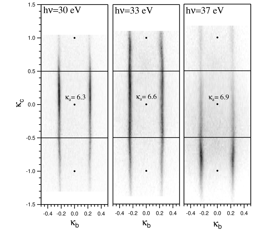
Figure 19: FS map at different photon energies $h\nu=$30, 33, 37 eV. For $\kappa_{b}$=$\kappa_{c}$=$0$, this is at $\kappa_{a}$=6.3, 6.6, and 6.9 as indicated. These figures have been stretched along $\kappa_{c}$ by a factor 1.7 (compare with FIG.s 11 and 20 (b), which are to scale).

Like in FIG. 17, the intensity for photoelectrons coming from slightly below the Fermi level is shown in FIG. 19, but now in the $\kappa_{b}\kappa_{c}$ plane, over two BZs $\left(\left|\kappa_{b}\right|\leq\frac{1}{2},\text{ }\left|\kappa_{c}\right|\lesssim 1\right),$ and for $h\nu=30,$ 33, and 37 eV. The coarse-grained intensity is seen to change significantly over this range of photon energies, and only for $33~{}$eV does it extend over both BZs. This we can partly understand from the $h\nu$-dependence of $\kappa_{a}$:

For the three photon energies, Eq. (104) yields respectively $\kappa_{a}\left(0,0,h\nu\right)=5.9$, 6.2, and 6.5, which according to the simplest prediction (95) of the $\kappa_{c}$-position of the intensity maximum (seen on the left-hand side of FIG. 16 for $\kappa_{a}$=6.0 and 6.8) for the $xy$ beam gives: $\kappa_{c}=0.5$, 0.2, and $-$0.1, as compared with 0.2, $\sim$0, and $-$0.6 estimated from the experimental FIG. 19. The latter $\kappa_{c}$-values correspond via Eq. (95) to the somewhat larger $\kappa_{a}$-values: 6.2, 6.4, and 7.0, whose intensity distributions can easily be imagined from those for $\kappa_{a}$=0 and 6.8 shown on the left-hand side of FIG. 16. These do exhibit the remarkable contraction along $\kappa_{c}$ of the experimental intensity distribution seen in FIG. 19 for the highest energy. On top of this comes the narrowing of the beam due the delocalization of the $\widetilde{xy}$ WO caused by the downfolding of the valence- and conduction-band orbitals [see Eq. III (109)].

X.4 CECs in the $\mathbf{b}^{\ast}\mathbf{c}^{\ast}$ plane

In FIG. 20 we present ARPES results for binding energies, $\omega,$ which takes us from the Fermi level to the bottom of the Mo $4d$-bands so that we also get to see the $xz$ and $yz$ valence bands. The results are shown in the 2D region $\left(0\leq\kappa_{b}\leq\frac{1}{2},\text{ 0}\leq\kappa_{c}\lesssim 1\right)$ which with reference to FIG.s 20 (a) and 11 includes the upper half of the BZ centered at $\Gamma_{00}\equiv\Gamma,$ plus the lower half of the one centered at $\Gamma_{01}\equiv\Gamma^{\prime},$ We shall refer to these BZs as respectively the 1st and the 2nd. Together, they form the upper part of the double zone centered at $\Gamma.$ Here, ”upper” and ”lower” refer to the orientation which has $\kappa_{c}$ pointing upwards.

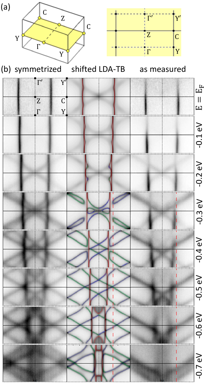
Figure 20: (a) Orientation in the zone of the $\kappa_{b}\kappa_{c}$-plane with $\kappa_{a}$=6. The CECs are shown in the upper part of the 1st and the lower part of the 2nd BZ: $\left|\kappa_{b}\right|\leq\frac{1}{2},$ $0\leq\kappa_{c}<1.$ See also FIG. 11. (b) Comparison of the CECs computed using the LDA-TB parameters, listed in Eq.s I (43)-(47) including the 100 meV shift, with those measured by ARPES for sample H ($T$=6 K, $h\nu$=30 eV). Red, blue, and green indicate dominating $xy,$ $xz,$ and $yz$ character. The red dashed line $\left(k_{b}\text{=0.225}\right)$ is the one along which we often show bands, such as the $\left|\mathbf{k}\right\rangle$-projected ones in FIG. 14. The match with the symmetrized ARPES is nearly perfect, and so is the prediction that in ARPES as measured, the $xz$ and $yz$ CECs are extinguished in the respective 2nd zone, i.e. above the respective $\mathrm{ZY}^{\prime}$ line. Indicated on the right are the energies with respect to the Fermi level.

The right-most panel in FIG. 20 (b) shows ARPES as measured and the left-most panel shows ARPES with the fine-grained (plus some of the coarse-grained) intensity variations symmetrized away by adding the intensities from both sides of the BZ boundary (CZC,$\,\kappa_{c}$=$\frac{1}{2}),$ exploiting the equivalence of $xz$ and $yz$. This corresponds to adding the intensities at $\mathbf{k}$ and $\mathbf{k+c}^{\ast}.$

The middle panel shows the CECs from the LDA-TB bands with the common energy of the four $xz$ and $yz$ WOs shifted downwards by 100 meV with respect to the energy of the two $xy$ WOs [see FIG.s 22 (a) and (b)] in order to improve the agreement with the symmetrized ARPES in the right-most panel. This agreement –down to every detail– is astonishing, and so is the straightness of the three sets of lines, even close to where they cross. The theoretical CECs have been colored red, blue, or green according to their respective $xy,$ $xz,$ or $yz$ character, and in order to mimic the spectral-function broadening of the dispersion, the shifted LDA-TB bands were broadened by a Lorentzian with energy-independent width.

The CECs from the symmetrized ARPES and the shifted LDA-TB bands behave as described in Paper I, Sect. IV.1.4 together with FIG.s 4, 6, 7, and 8. The upper part of the double zone is shown also in FIG. 11 of the present paper.

In FIG. 20 we recognize the CECs of the quasi-1D, degenerate $xy\left(\mathbf{k}\right)$ and $xy\left(\mathbf{k+c}^{\ast}\right)$ bands (red) dispersing in the $k_{b}$ direction with the distance $2k_{b}\left(E\right)$ between the two sheets increasing like $\sim\left(2/\pi\right)\sqrt{\left(E-B\right)/\left|t\right|}$ with $t\sim-1~{}$eV [see Sect. IV.1 Eq. I (23)] and heading towards $\sim\frac{1}{2}$ at the Fermi energy.

The quasi-1D $xz\left(\mathbf{k}\right)$ (blue) and $yz\left(\mathbf{k}\right)$ (green) bands dispersing with respectively $k_{c}-k_{b}$ and $k_{c}+k_{b}$ [see Eq. I (27)], are degenerate at their common bottom at $\Gamma$ where they are also nearly degenerate- and hybridize with the two $xy$-bands thus giving rise to CECs which are complicated near $\Gamma.$ For energies a bit above the common bottom of all three $t_{2g}$ bands, $B\approx E_{F}-0.75$ eV, the blue and green pair of CECs are parallel with and lie on either side of respectively the $k_{c}-k_{b}=0$ and $k_{c}+k_{b}=0$ lines. As the energy increases, so does the distance $\sim\left(2/\pi\right)\sqrt{\left(E-B\right)/\left|A_{1}\right|}$ between each pair of parallel blue or green CECs. This distance is approximately $\sqrt{t/A_{1}}\sim 1.8$ times the one between the red $xy$ CECs.

The blue and the green $\mathbf{k+c}^{\ast}$-bands are shifted by $\Delta k_{c}$=$1$ and thus behave in the same way as the respective blue and green $\mathbf{k}$-bands. For energies above $\sim-0.5$ eV, the closest CEC pairs are those on either side of the respective zone boundary, $\left|k_{c}+k_{b}\right|=\frac{1}{2}$ or $\left|k_{c}-k_{b}\right|=\frac{1}{2},$ onto which they coalesce when $E\sim E_{F}-2\left|G_{1}\right|=E_{F}-0.2\,$eV. Here, 2$G_{1}$ is the electronic dimerization causing a gap of $\pm 2G_{1}$[see Eq. I (29) and FIG. I 6 for $k_{b}$=0.225].

We are particularly interested in the hybridization of the $xy$-bands inside the gap around $E_{F}.$ It can be seen in theory by comparison of the light- and the dark red bands in FIG. I 6 and I 7, respectively, or in the middle and bottom parts of FIG. 14 of the present Paper II, and we shall study it in detail in Paper III. Although bands –and not CECs– hybridize, we can see the effect of this hybridization in the LDA-TB part of FIG. 20 at 0.1 and 0.2 eV below $E_{F}$ as four ”notches” pointing inwards, towards Z, and we can follow them as the energy is lowered into the valence bands. The origin of the notches is clearly the energy repulsion between the hybridizing valence-band edge and one of the two degenerate $xy$-bands; the other band is unaffected. Since the notch is sharp, it can only come from an edge of a nearby $yz$- or $xz$-band (but not from a far-away $yz$- or $xz$-band) with a weak matrix element, and as long as the notch points towards Z rather than Y, it comes mainly from the edge of the valence (V) rather than from the edge of the conduction (C) band. The corresponding peak is in the upper $\widetilde{xy}$ band (FIG. I 7) and we shall call it a resonance peak. (If we take the nearly dispersionless $k_{a}$-dimension into account, the peak is a ”mountain ridge” extending along $\mathbf{a}^{\ast})$.

According to the selection rules derived in Sect. IX.2.1 and illustrated in FIG. 14, ARPES as measured in FIG. 20 (b) should see the occupied $\left|\mathbf{k}\right\rangle$-projected bands in the 1st physical zone and the occupied $\left|\mathbf{k+c}^{\ast}\right\rangle$-projected bands in the 2nd physical zone. With the blue $xz$- and green $yz$-bands gapped around the Fermi level, these bands should be seen in the 1st physical zone only, and comparison with FIG. 11 shows this to be the case. Specifically, the blue and green bands with $E<E_{F}-0.2~{}$eV are extinguished in their respective 2nd zone. The dimerization distortion of the $yz$ (and $xz$) intensities for negative $\kappa_{c}$ predicted in FIG. 13 for $\kappa_{a}$=6.4, specifically the intensity enhancement near $\kappa_{c}$=–0.4 for the upper band was seen in the data; but this is outside the range of positive $\kappa_{c}$ shown in FIG. 20 (b).

For the red, metallic $xy$-bands, the Fermi sea inside the outer sheet should be seen in the 1st BZ and the sea inside the inner sheet should be seen in the 2nd BZ, with a switch near the BZ boundary, $k_{c}$=$\frac{1}{2}.$ This means that the notches should be seen only in the 2nd BZ, but the drop of intensity for $\kappa_{c}>0.5$ in ARPES as measured with $h\nu$=$30~{}$eV (FIG. 19) makes this observation difficult. We shall return to it in Sect. III XV.

Herewith, we have arrived at the influence of the $yz$ and $xz$ form factors. In FIG. 20 (b) we see that the intensity as measured for given binding energy (deep inside the valence bands) is slightly stronger for $yz\left(\mathbf{k}\right)$ than for $xz\left(\mathbf{k}\right)$ and increases with $\kappa_{c}$ in the range $\left(0|1\right)$. As may be seen from the theoretical FIG. 16, the former property is consistent with the behavior of $\kappa_{a}^{2}\left|w_{yz}\left(\mathbf{\kappa}\right)\right|^{2}$ for $\kappa_{a}\sim 6.4$, but the latter requires $\kappa_{a}\sim 7$ .

X.5 Energy bands $E_{j}\left(k_{b},k_{c}\right)$

In the preceding section, the CECs as measured were shown in the right-hand panel of FIG. 20 (b) and were explained as the fine-grained, double-periodic $\left|\mathbf{k}\right\rangle$-projection of the occupied part of the lower $m$-band in the 1st- and of the upper $m$-band in the 2nd physical zone (see Sect. IX.2.1), on the background of the coarse-grained, aperiodic polarization- and WO form factor intensity $\kappa_{a}^{2}\left|\tilde{w}_{m}\left(\mathbf{\kappa}\right)\right|^{2}$ (see Sect. IX.2.2). Hence, the $xz$ and $yz$-bands were seen only in the respective 1st physical zone, because their upper bands are empty, and so were the metallic $xy$-bands due to the drop of their polarization- and form factor intensity for $h\nu$=30 eV ($\kappa_{a}$=6.3$)$ in the 2nd BZ.

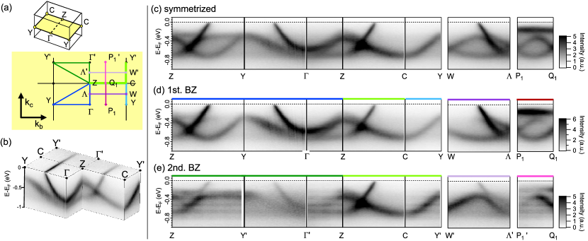
Figure 21: ARPES band structure. (a) Orientation of half the 1st BZ in $\kappa_{a}\kappa_{b}\kappa_{c}$-space and, in the $\kappa_{b}\kappa_{c}$-plane, half the 1st BZ $(0\leq\kappa_{c}\leq\frac{1}{2})$ centered at $\Gamma$, and half the 2nd BZ $\left(\frac{1}{2}\leq\kappa_{c}\leq 1\right)$ centered at $\Gamma^{\prime}$. The BZ is the physical zone for the $xy$-bands and the physical zones for all three $t_{2g}$-bands were shown in FIG. 11. (b) Data as measured from sample H ($T$=6 K, $h\nu$=30 eV) presented in an $E\left(\kappa_{b},\kappa_{c}\right)$-box where from cuts along the $\kappa$-paths colored in (a) produce the band structures shown in (c)-(e). (d) Some features can be better seen in the 1st BZ, (e) while others are more pronounced in the 2nd BZ, and vice versa. This is so because band selection follows the physical- rather than the Brillouin zone. (c) The symmetrized band structure shows all spectral features.

FIG. 21 (b) now displays the ARPES band structure as measured on the faces of a box with the basal $\left(k_{b},k_{c}\right)$ plane extending over the upper half of the double zone, like in FIG.s 20 and 11. On the top face, i.e. for $E\sim E_{F},$ we recognize the 1D $xy$ FS, $\left(k_{b},k_{c}\right)\sim\left(\pm\frac{1}{4},k_{c}\right),$ with its intensity drop in the 2nd BZ. Not only the $xy$-bands are quasi 1D, but so are the $xz$ and the $yz$-bands: Had the box been cut at the top of the valence bands, we would –like in the right-most panel of FIG. 20 (b)– have seen their ridges follow the boundaries of their physical zones (FIG. 11).

The band structures shown in (d)-(e) are obtained by cutting the data along the lines colored in (a). In order to avoid the fine-grained intensity variations, we first show (c) –like in the left-most panel of FIG. 20 (b)– the band structure symmetrized over the 1st and 2nd zones; the benefit of this symmetrization is evident! Had there been no coarse-grained intensity variations, this band structure would have been periodic in the BZ and have the rectangle $\mathrm{\Gamma ZCY}$ $\left(0\leq k_{b}\leq\frac{1}{2},0\leq k_{c}\leq\frac{1}{2}\right)$ as its irreducible part. The symmetrized bands (c) will be compared with the LDA band structure (FIG. 22) in the following Sect. XI and, subsequently, its TB parameters will be fine-tuned to achieve almost perfect agreement with the occupied ARPES bands.

The fine-grained intensity variations, on the other hand, hold the key to resolving the sofar elusive splitting and warping of the nearly degenerate quasi-1D $xy$-like FS. But let us first test our understanding of the intensity variations, by using it to explain the band structure as measured along the lines colored in FIG. 21 (a) and shown in FIG.s (b), (d), and (e).

Along $\mathrm{\Gamma Z\Gamma}^{\prime}$ $(k_{b}$=0$)$ we see the rise of the degenerate $xz\left(\mathbf{k}\right)$ and $yz\left(\mathbf{k}\right)$ valence bands from their bottom at $E_{F}-0.75~{}$eV at $\Gamma$ to their highest point, $E_{F}-0.25~{}$eV, where the blue and green valence-band ridges cross at $\mathrm{Z.}$ Here, half their $\left|\mathbf{k}\right\rangle$ characters –and hence ARPES intensities– have been lost. On the downturn in the 2nd zones, to $\Gamma^{\prime}$, the $\left|\mathbf{k+c}^{\ast}\right\rangle$ characters take over and the intensities drop accordingly. At $E_{F}-0.75~{}$eV we also see the dispersionless bottom of the two degenerate $xy$-bands and expect the intensity to shift from the lower to the upper band as we pass from the 1st to the 2nd BZ. That the measured total $xy$ intensity nevertheless drops, we ascribe to the above-mentioned drop of the form factor in the 2nd BZ.

When going inside the 1st zone from $\mathrm{\Gamma}$ to $\mathrm{Y}$, the other crossing point of the blue $xz$ and green $yz$ valence-band ridges (see FIG. I 8 or II 11), the $xz\left(\mathbf{k}\right)$ and $yz\left(\mathbf{k}\right)$ valence bands are seen to rise and lose intensity in a similar same way as they did towards $\mathrm{Z}$, except that there –due to spin-orbit splitting (see FIG. 23)– the maximum was higher. The $\mathrm{\Gamma Y}$-cut in the band structure is also shown on the front face of the box in (b). Intensity is prominently seen from the (lower) $xy$-band rising parabolically from its bottom along $\Gamma\mathrm{Z}$ to the FS along $k_{b}\approx\frac{1}{4}$. The aforementioned drop of $xy$ intensity in the 2nd BZ is clearly seen on the top face of the box. If we go inside the 2nd zones from $\Gamma^{\prime}$ to $\mathrm{Y}^{\prime}$ at the zone boundary, this is the only place where intensity from the valence bands is seen.

Along the green diagonal from $\mathrm{Y}^{\prime}$ to $\mathrm{Z,}$ where the gapped $yz\left(\mathbf{k}\right)$- and $yz\left(\mathbf{k+c}^{\ast}\right)$-bands form the valence-band ridge, this ridge is clearly seen; in fact far better than the blue ridge from $\mathrm{Y}$ to $\mathrm{Z}$ formed by the gapped $xz\left(\mathbf{k}\right)$- and $xz\left(\mathbf{k+c}^{\ast}\right)$-bands. A similar intensity difference between $yz$ and $xz$ was also observed in FIG. 20 and was explained at the end of Sect. X.4 as due to different form factors. The $xz$-band gives no intensity along the green $\mathrm{Y}^{\prime}\mathrm{Z}$ line because it is in the 2nd $yz$ zone, which is empty. Returning now to the blue valence-band ridge along $\mathrm{YZ,}$ we see the $yz$-band fall, reach its bottom halfway towards $\mathrm{Z,}$ and then rise again to the highest point on the ridge at $\mathrm{Z.}$ Here, the $yz$-band not only attains $\left|\mathbf{k+c}^{\ast}\right\rangle$ character, but also hybridizes with the $xz$-band via spin-orbit coupling. We also see the parabolic rise of the lower $xy$-band from its bottom at $\mathrm{Z}$ towards $\mathrm{Y}$, reaching $E_{F}$ at half the way. Towards $\mathrm{Y}^{\prime},$ the $xy$ intensity is reduced by the form factor.

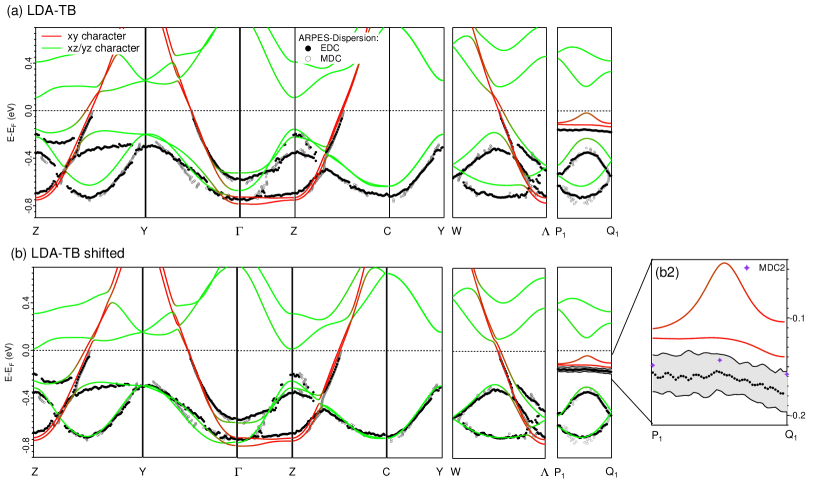
Figure 22: ARPES (black dots and grey circles) and LDA ($xy$ red and $xz/yz$ green) band structures. The line P₁Q₁ has $k_{b}$=0.225 and $k_{c}$=0 to 0.5, see FIG.s 11, 20, and 21 (a). The experimental bands come from the symmetrized ARPES measurements ($T$=6K, $h\nu$=30 eV) on sample H whose metallic bands are 51% filled (see Sect. XV.2 in Paper III) and displayed in FIG.  21 (c). They were determined by searching the intensity maximum along the direction of either energy (EDC, black dots) or momentum (MDC, grey circles). (a) The LDA bands are the eigenvalues of the six-band TB Hamiltonian defined in Sect. I  VI with the parameters listed in Tables I (43)-(47) and (49). (b) As above, but with the energy of the $xy$ WOs shifted 100 meV upwards. The blow-up along P₁Q₁ in (b2) compares the shifted LDA-TB theory with the experimental band (black dots with uncertainty in grey). The diamonds, labeled ’MDC2’, indicate the band determined from the maximum along the momentum direction $\mathbf{b}^{\ast}$ perpendicular to $\mathrm{P}_{1}\mathrm{Q}_{1},$ where the band disperses strongly.

Going along the BZ boundary from $\mathrm{Z}$ to $\mathrm{C}$ for $k_{b}$ positive, the nearly degenerate $xy$-bands rise and cross the Fermi level near $\left(\frac{1}{4},\frac{1}{2}\right)$ and the $xz\mathbf{\ }$valence band falls from the highest point on the ridge to its bottom at $\mathrm{C.}$ At $\mathrm{Z,}$ the green $yz$-band is degenerate with the blue $xz$ valence band and has intensity there, which however vanishes after leaving the 1st green zone.

Upon going from $\mathrm{C}$ to $\mathrm{Y}^{\prime}$ ($k_{b}$=$\frac{1}{2})$ inside the blue $xz$ zone, we see the $xz$-band increase to the blue ridge at $\mathrm{Y}^{\prime}$. Going instead to $\mathrm{Y,}$ we see the other branch of the $xz$-band increase to the blue ridge at $\mathrm{Y.}$

Along $\mathrm{\Lambda W}\,$($k_{c}$=$\frac{1}{4}$), the lowest band –with minimum at ($\frac{1}{4}$,$\frac{1}{4}$)– is the blue $xz\left(\mathbf{k}\right)$-band. The $yz\left(\mathbf{k}\right)$-band is degenerate with $xz\left(\mathbf{k}\right)$ at $\Lambda,$ but then increases, until at ($\frac{1}{4}$,$\frac{1}{4}$) it reaches the top of the green $\mathrm{ZY}$ ridge where it mixes with the $yz\left(\mathbf{k+c}^{\ast}\right)$-band coming from $\mathrm{W,}$ and thereby looses its intensity. Going instead from $\mathrm{\Lambda}^{\prime}$ towards $\mathrm{W}^{\prime}\mathrm{\ }$($k_{c}$=$\frac{3}{4}$), it is the blue $xz\left(\mathbf{k+c}^{\ast}\right)$-band which –with weak intensity– increases until at ($\frac{1}{4}$,$\frac{3}{4}$) it reaches the top of the blue $\mathrm{ZY}^{\prime}$ ridge where the $\left|\mathbf{k}\right\rangle$ character takes over and the $xz\left(\mathbf{k}\right)$-band continues with full intensity downhill. The lower $xy$-band disperses parabolically upwards from $\mathrm{\Lambda}$ and reaches the Fermi level half the way to $\mathrm{W,}$ and the same is seen –with reduced intensity– along $\mathrm{\Lambda}^{\prime}\mathrm{W}^{\prime}\,$($k_{c}$=$\frac{3}{4}$) for the higer $xy$-band. The non-vanishing hopping integrals I (46) between an $xy$ WO and an $xz$ or $yz$ WO causes the corresponding bands to repel where they run close. This is the case for the two $xy$-bands and the $yz\left(\mathbf{k}\right)$ band between $\Lambda$ and $\left(\frac{1}{4},\frac{1}{4}\right),$ and for the two $xy$-bands and the $xz\left(\mathbf{k}\right)$-band between $\Lambda^{\prime}$ and $\left(\frac{1}{4},\frac{3}{4}\right).$ It is remarkable that of the three close bands, two repel around the third band, which remains unaffected and thereby ends up as the band of intermediate energy, the lowest of the two $xy$-bands in the present case. This can be seen in FIG. 21 (c)-(e) and will be referred to often in the following.

The $\mathrm{P}_{1}\mathrm{Q}_{1}\mathrm{P}_{1}^{\prime}$-line ($k_{b}$=0.225) is perpendicular to the $\mathrm{\Lambda W}$ and $\mathrm{\Lambda}^{\prime}\mathrm{W}^{\prime}$ lines and is parallel to, but slightly inside the FS so that the trace of the $xy$-bands is $\mathrm{\sim}170$ meV below the Fermi level and thereby clearly visible in ARPES –albeit with the usual $xy$ form-factor reduction of the intensity towards $\mathrm{P}_{1}^{\prime}$. Starting from $\mathrm{P}_{1},$ we see the blue $xz\left(\mathbf{k}\right)$-band reaching its bottom midways to $\mathrm{Q}_{1}$ and –above it, with slightly less intensity,– the green $yz\left(\mathbf{k}\right)$-band rising towards the top of the green ridge where 50% of its character and intensity are lost and losing even more on the downhill side towards $\mathrm{Q}_{1}$. Proceeding from here towards $\mathrm{P}_{1}^{\prime}$ in the 2nd green zone, we vaguely see the green $yz$-band –now $\left|\mathbf{k+c}^{\ast}\right\rangle$-like– reach its bottom midways to $\mathrm{P}_{1}^{\prime}.$ From $\mathrm{Q}_{1}$ in the blue 1st zone, we see the blue $xz$-band rise to the $\mathrm{ZY}^{\prime}$ ridge, where it –like the green $yz$-band at the green ridge– has lost half its intensity and thereafter vanish on the downhill side towards $\mathrm{P}_{1}^{\prime}.$ All of this agrees with the $\left|\mathbf{k}\right\rangle$ characters of the four lowest LDA-TB bands shown at the bottom of FIG. 14 and, at the top, with the $xy$ form-factor dropping in the 2nd BZ thus hiding the resonance peak predicted to exist in the upper $\widetilde{xy}$-band.

Before attempting to extract ARPES data beyond the 100 meV scale, we need to assess the degree of agreement between the LDA and the ARPES dispersions.

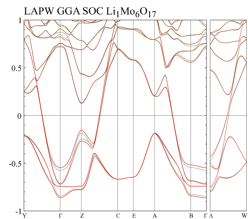
Figure 23: Relativistic LAPW GGA control calculation of the LiPB band structure using the Perdew–Burke–Ernzerhof (PBE) functional [85]. We show the bands along the same lines in the BZ as shown at the top of FIG. I 3 whose bottom shows the 336 NMTO LDA band structure. The 6 NMTO TB band structure in the Y$\Gamma$ZC plane is shown in FIG. I 4. LAPW band energies are in eV with respect to $E_{F}.$ Red bands are with- and grey bands are without spin-orbit coupling. We see that the crossings between the 3rd and 4th bands along $\mathrm{\Gamma Z}$ and $\mathrm{ZC}$ and between the 1st and 2nd bands between $\mathrm{Y\Gamma}$ and $\mathrm{AB}$ are spin-orbit split by about $80$ meV.

XI Agreement between ARPES and the LDA

The band structure derived from the symmetrized ARPES data is shown in FIG. 22 (a) and (b). The points indicated by grey circles were extracted from the peak locations in the momentum distribution curves (MDCs), $I(|\mathbf{k}|$ in a specified direction, fixed energy $E)$, and the points indicated by black dots were extracted from peak locations in energy distribution curves (EDCs), $I$(fixed $\mathbf{k},E)$. The peak maxima in these curves were found from the zeros in the smoothed first derivative with respect to $|\mathbf{k}|$ for an MDC, or $E$ for an EDC, under the condition that the smoothed second derivative is smaller than zero.

The bands resulting from the first-principles LDA calculation (in the TB representation of the six $t_{2g}$ WOs; see Sect. V in paper I) are shown in (a), with the sum of the $xz$ and $yz$ characters in green and the $xy$ character in red. Note the strong hybridization of the nearly degenerate bottoms of the two $xy$ and the $xz$ and $yz$ valence bands near $\Gamma.$ Note also the hybridizations between $\mathrm{Z}$ and $\mathrm{Y}$ and between $\mathrm{W}$ and $\mathrm{\Lambda.}$ Near the middle of the latter line where the two degenerate $xy$-bands in the gap come close to the valence and conduction (V&C) bands, and their repulsion is therefore strong –but in opposite directions– one of the $xy$ states stays unaffected and the other is pushed up or down in energy, depending on whether the repulsion from the valence or the conduction band is stronger. Since this balance tips as we move up through the gap, the hybridization shifts from the upper to the lower $xy$-band and causes the resonance peak to shift from upwards pointing in the upper band, to downwards pointing in the lower band. The fact that the matrix element, $\alpha\left(\mathbf{k}\right)+a\left(\mathbf{k}\right),$ for hybridization of the $xy$- and $xz/yz$-bands decreases with increasing $k_{b}$ causes the rather strange-looking dispersion of the two $xy$-bands along $\Lambda\mathrm{W}$. This asymmetry will be explained in Sect. III XIV.2; specifically, in connection with Eq. III (XIV.1.2) and with the left-hand sides in the 6th row of FIG. III 26. Along $\mathrm{P}_{1}\mathrm{Q}_{1}$, we clearly see the resonance peak in the upper $\widetilde{xy}$-band.

XI.1 Shifting the LDA $xz$- and $yz$-bands downwards with respect to the $xy$-bands

Overall in FIG. 22 (a), there is good agreement with the occupied ARPES bands, the main discrepancy being that the LDA valence bands lie 100 meV too high with respect to the $xy$-bands and thereby with respect to the Fermi level. This may be partly a surface effect: The $xz$ and $yz$ WOs reach farther into the vacuum and therefore feel a higher LDA potential than the $xy$ WOs which are well inside the staircase. In addition, there is undoubtedly an LDA error; for instance, LDA bandgaps in semiconductors are too small, and FS measurements for bulk $4d$ metals indicate that the accuracy with which the LDA describes the energy separation between inequivalent $t_{2g}$ levels is $\sim$50 meV. For LiPB, we therefore correct the bulk LDA bands by shifting the energy of the green V&C bands downwards by 100 meV [more precisely, we shift the on-site energy, $\tau_{0},$ of the $xy$ and $XY$ WOs 100 meV upwards, i.e. from 47 to 147 meV in Table I (43), with respect to the common on-site energy of the $xz,XZ,yz,$ and $YZ$ WOs, and subsequently recalculate the Fermi level]. The result shown in (b) agrees very well with ARPES, as was seen already in FIG. 20$\,($b$)$ for the CECs. An exception is near $\mathrm{Z,}$ where the splitting of the valence band is too small and the lowest conduction band nearly touches the Fermi level, thus asking for a fine-adjustment of the TB parameters.

The LDA and ARPES band structures in FIG.s 22 (a) and (b), are lined up with respect to the Fermi level, which for the LDA calculation for stoichiometric LiMo₆O₁₇ corresponds to 50% filling of the metallic bands. In the experiment, Li and O vacancies make the filling uncertain and is estimated from the measured $k_{Fb}$ value (Sect. III XV) to be $51\pm 1$ $\%,$ i.e. to have the effective stoichiometry Li_1.02±0.02. Using the measured Fermi-velocity, this then gives a Fermi level which with respect to the band structure is between 50 and 0 meV above the level for the stoichiometric crystal assumed in the calculation, which means that the metallic ARPES bands could lie 50 to 0 meV below the LDA bands in FIG. 22 (b). But this can only account for the $\sim$40 meV distance to the lower LDA $\widetilde{xy}$-band seen in a direction perpendicular to $\mathbf{b}^{\ast},$ such as along $\mathrm{P}_{1}\mathrm{Q}_{1},$ in particular in the blow up (b2).

The black dots in (b2) were obtained as the position of the EDC maxima (one for each $\mathbf{k}$) and the grey area indicates the uncertainty of the experiment, as well as the uncertainty in determining the position of the one EDC maximum. The three purple diamonds labeled ’MDC2’ are from MDCs along respectively $\mathrm{\Gamma Y,}$ $\Lambda\mathrm{W,}$ and $\mathrm{ZC}$, perpendicular to $\mathrm{P}_{1}\mathrm{Q}_{1}.$

The upper $\widetilde{xy}$-band predicted by the LDA, seems to be missing in the symmetrized ARPES data (b2). This, we can understand by going back to the ARPES bands ”as-measured” along $\mathrm{P}_{1}\mathrm{Q}_{1}\mathrm{P}_{1}^{\prime}$ in FIG. 21 (d) and (e) where intensity just below the Fermi level was seen in the 1st- but hardly in the 2nd BZ. As illustrated in FIG. 14, the lower $xy$-band is selected in the 1st- and the upper band in the 2nd BZ. Since for $k_{b}$=0.225, the $xy$-bands are closer to the valence than to the conduction bands, the repulsion from the former dominates and pushes a resonance peak up in the upper band. This peak thus has ARPES intensity in the 2nd zone where it gets strongly reduced by the $xy$ form factor. The symmetrization of the $\mathrm{P}_{1}\mathrm{Q}_{1}$ and $\mathrm{Q}_{1}\mathrm{P}_{1}^{\prime}$ ARPES data finally adds to hiding the band in the 2nd BZ behind the one seen in the 1st BZ, and that is the reason why in FIG. 22 (b2) only the lower ARPES band is seen. From the ARPES data, we can therefore only uncover the upper $\widetilde{xy}$ band if we avoid the symmetrization.

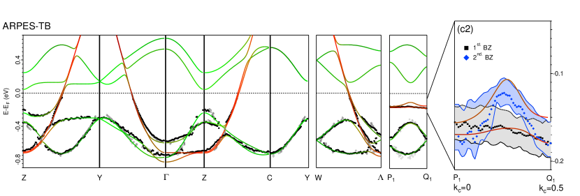
Figure 24: Band structure obtained as the eigenvalues of the six-band TB Hamiltonian, Eq.s I (35) or I  (56), with parameter values fine-tuned to improve the fit to the ARPES bands and given in the square parentheses in Tables I (43)-( 47). The Fermi level is $\sim$0.1 eV above the center of the gap [see text following Eq. I (49)]. The ARPES data here are those already shown in FIG. 22, except for those in the blow-up (c2) along $\mathrm{P}_{1}\mathrm{Q}_{1}$ ($k_{b}$=0.225), which are non-symmetrized EDC data from respectively the 1st (black) and 2nd BZ. The latter data is subsequently mirrored around the $k_{c}$=0.5 zone boundary into the 1st BZ (blue).

XI.2 Fine-tuning the TB Hamiltonian and extracting both quasi-1D bands from ARPES as measured

Our first-principles LDA TB description of the six lowest energy bands given in Sect. I VI has about 40 TB parameters (WO energies and hopping integrals). Their LDA values, derived as described in Sect. I II, are given in Tables I (43)-(47) and yield the band structure shown in FIG. 22 (a). As explained above, the improved agreement with ARPES seen in (b) was achieved by merely shifting the value of $\tau_{0},$ the energy of the degenerate $xy$ and $XY$ WOs, up with respect to that of the degenerate $xz,$ $XZ,$ $yz,$ and $YZ$ WOs. The latter is the energy at the center of the gap and is taken as the zero of energy in the TB Hamiltonian. Still, the Fermi velocity is too small and the resonance peak along P₁Q₁ is too high. Moreover, the levels near $Z,$ where the V&C bands come closest, remain inaccurate: the splitting of the valence band levels is too small while that of the conduction band levels is too large. This is due to bad convergence and truncation of the $xz$-$yz$ hybridizations I (40), to our neglect of the spin-orbit coupling in the NMTO –but not in the LAPW (FIG. 23)– calculation, and to the LDA yielding too small a gap.

We therefore refined the parameter values, with the results given in square parentheses in Tables I (43)-(47). Specifically, we found it necessary to modify the values of the intra-ribbon hopping integrals, first of all, between respectively the on-site, 1st-, and 2nd-nearest $xy$ WOs, $\tau_{0},$ $\tau_{1},$ and $\tau_{2}.$ This increases the Fermi velocity by about 15%, increases the upward curvature of the bands near half filling, and lowers the half-filling Fermi level to 53 meV above the center of the gap; see Eq.s I (43) and I (VI.1)-(50) in Sect. I VI. Secondly, we refined the values of the $xz$-$yz$ hopping integrals, $m_{1},$ $\lambda_{2},$ and $\lambda_{3}$ in Eq. I (47). In addition, the value of the gap parameter, $G_{1}$, originating in the asymmetry (dimerization) between the forwards and backwards hoppings, $xz\leftrightarrow XZ$ $\left(yx\leftrightarrow YZ\right),$ as explained after Eq. I (27) and given in Eq. I (45), was increased by 10%. The resulting band structure is displayed in FIG. 24 and is seen to agree almost perfectly with the experiment.

Most importantly, we have succeeded in extracting both metallic bands by using the ARPES data as measured along $\mathrm{P}_{1}\mathrm{Q}_{1}\mathrm{P}_{1}^{\prime}$ ($k_{b}$=0.225) for the EDCs. These ARPES bands are displayed in the blow-up (c2) where the band obtained in the 1st zone from $\mathrm{P}_{1}$ to $\mathrm{Q}_{1}$ has been plotted in black squares with the uncertainty in grey, and the band obtained in the 2nd zone from $\mathrm{Q}_{1}$ to $\mathrm{P}_{1}^{\prime}$ has been plotted in reverse order, from $\mathrm{Q}_{1}$ to $\mathrm{P}_{1}$ in the 1st zone, and in blue. Even though the 2nd BZ emission is relatively weak in this h$\nu$=30 eV data (recall from Sec. X.3.2), nonetheless, we now see at mid-zone the resonance peak in the blue upper band, well separated from the grey lower band, while near $k_{c}$$=0$, $0.5$, and $1$, the splitting of the two bands is less clear. The reasons for the latter are technical:

1) The extraction was done by assuming only one (possibly broad) maximum per EDC whereby in the zone-boundary (ZB) region $\left(0.4<k_{c}<0.6\right)$ where both bands have a significant $\left|\mathbf{k}\right\rangle$ projection, only one band is found (see red bands in the middle and bottom parts of FIG. 14). In FIG. III 32 we shall see an example of how the one-peak extraction method switches between the two bands when the ZB is crossed.

2) With the ARPES intensity fading away upon approaching $k_{c}$$=$$1$ ($\mathrm{P}_{1}^{\prime}$) smoothening the EDCs before taking the derivative (to locate the maximum) pushes the intensity to increasingly higher binding energies, $\omega,$ and thereby causes the band near $\mathrm{P}_{1}^{\prime},$ which is the (blue) upper band, to fall below the one near $\mathrm{P}_{1},$ which is the (grey) lower band.

FIG. 24 thus demonstrates that the refinement of merely 7 out of the more than 40 TB parameters to fit the ARPES bands, lying more than 0.15 eV below the Fermi level, achieves nearly perfect agreement also for the $k_{c}$-dispersion of the quasi-1D bands closer to the Fermi level. This includes agreement with the size and shape of the resonance peak in the upper band, without having modified any of the 17 $\left(a,g,\alpha,\gamma\right)$-parameters I (46) describing hybridization between the $xy$ and the $xz$- and $yz$-bands. This clearly shows the decisive role that resonant coupling to the gapped $xz$ and $yz$-bands plays in determining the splitting and dispersion of the metallic $xy$-bands.

Besides the above-mentioned peculiarities and experimental uncertainties, the agreement between ARPES and the refined TB bands is astonishingly good. In both cases, the peak caused by the resonance with the $xz$ valence band at $\left(k_{b},k_{c}\right)$=(0.225, 0.725) –mirrored around the $k_{c}$=0.5 line to the resonance with the $yz$ valence band at (0.225, 0.275)– comes out clearly in the upper $\widetilde{xy}$-band, and so does the lack of a visible resonance peak in the lower band at (0.225,0.275).

XI.3 True Value of the Fine Tuning Fit

While it is intrinsically very satisfying to obtain a good fit to the ARPES data, the true value of the fit is the very fact that it was possible to do. Thus we know that our analytic TB representation of the bands, as inferred from the LDA results, is fundamentally correct at the qualitative level, and is not missing any essential underlying physics. Otherwise, merely varying the magnitudes of parameters could not achieve a good fit. In particular, as emphasized already, obtaining a good description of the low-energy FS features by fitting only the high-energy features serves to validate our essential insight that the details of these FS features do indeed result from their couplings to the higher energy valence and conduction bands.

Therefore we proceed to use the refined TB model in the following Paper III to focus on the metallic $\widetilde{xy}$-bands in the gap, the origins of their observed $k_{c}$-dispersion on the 10 meV-scale, and their $k_{c}$-dispersion as a function of their position in the gap, i.e. of the $k_{b}$-value. This will enable us to study the details of the FS. We shall see that the theoretical splitting between the two metallic bands near the $|k_{c}|$=0.5 zone boundary increases as the energy moves away from the valence - and towards the conduction band. With the h$\nu$=33 eV data (see FIG. 19) the zone-selection rule, and a detailed analysis of our high-resolution data, we shall be able also with ARPES to separate the two FS sheets.

XII Summary and Outlook

In Sect. IX of this Paper II we derived a one-electron theory of the ARPES intensity variations in LiPB, which was then used in Sect. X to understand and analyze the extensive data presented there.

For the intensity of photoemission with momentum $\mathbf{\kappa}$ and binding energy $\omega$ $\left(\geq 0\right),$ we used the one-step expression (IX.1) with the least specific choice, plane waves $e^{2\pi i\mathbf{\kappa\cdot r}},$ for the final states, and approximation (71) for the matrix element. As a basis for the initial states, we used the six $t_{2g}$ WOs, $w_{m}\left(\mathbf{r}\right)$ and $W_{m}\left(\mathbf{r}\right),$ centered on respectively Mo1 and MO1, the most central molybdenums of the lower and the upper strings, ${}^{\text{Mo2}}\diagdown_{\text{Mo1}}\diagup^{\text{Mo4}}\diagdown_{\text{Mo5}}$ and ${}^{\text{MO5}}\diagdown_{\text{MO4}}\diagup^{\text{MO1}}\diagdown_{\text{MO2}},$ shown in FIG. I 2 (a). Due to the approximate translational equivalence [see Eq.s I$\,($17$)$ and (18)] of $w_{m}\left(\mathbf{r}\right)$ and $W_{m}\left(\mathbf{r}\right),$ the photoemission intensity is essentially the projection of the initial-state band with energy $E\left(\mathbf{k}\right)=E_{F}-\omega,$ onto the pseudo Bloch sum, $\left|w;\mathbf{k}\right\rangle$ in Eq. I (52) with $\mathbf{k=\kappa-G}$ in the double zone (see FIG.s 11 and FIG. 14 bottom). This would have been the initial-state band had the vector distance between Mo1 and MO1 been $\frac{\mathbf{c+b}}{2},$ rather than $\frac{\mathbf{c+b}}{2}-\mathbf{d,}$ and had $W\left(\mathbf{r}\right)$ been equal to $w\left(\mathbf{r}\right),$ rather than inverted around $\frac{\mathbf{c+b}}{2}-\mathbf{d.}$ For a band with dominant $m$ character, we thus expected that ARPES will see the lower band if $\mathbf{\kappa}$ is in the 1st physical zone, and the upper band if $\mathbf{\kappa}$ is in the 2nd physical zone and the band is occupied. Specifically, that the relative intensity of emission from the $\genfrac{}{}{0.0pt}{}{\mathrm{upper}}{\mathrm{lower}}$ $m$ band is $\frac{1}{2}\left[1\mp\cos\phi\right],$ where $\phi_{m}\left(\mathbf{k}\right)$ is given by the $m$-band structure in Eq. I$\,($62$).$ Taking now the $c$-axis dimerization into account, we found that this expression is modified to: $\frac{1}{2}\left[1\mp\cos\left(\phi-\eta\right)\right],$ where $\eta_{m}(\mathbf{\kappa)\equiv}$ $2\arg\tilde{w}_{m}\left(\mathbf{\kappa}\right)-2\pi\mathbf{\kappa\cdot d}$ is the difference between the phase shifts due to the inversion- and displacement dimerizations. These phase shifts were shown in the 1st column of FIG.s 12 and 13 for respectively the $xy$ and $yz$-bands. Whereas the inversion phase shift depends stronger on $\mathbf{\kappa}$ for the $yz$ WO than for the more structurally protected $xy$ WO, the displacement phase shift is independent of $m$ and rather constant. We had therefore expected the selection rule to hold better for the $xy$-bands. However, in both cases and with $\kappa_{a}$ (which does not influence the band structure) suitably chosen via the photon energy, the inversion- and displacement phase shifts tend to cancel with the result that the selection rule holds surprisinly well, provided that $\kappa_{a}$ is properly chosen. This was seen in the 2nd column of FIG.s 12 and 13.

On top of this fine-grained structure of the photoemission intensity, there is a coarse-grained aperiodic structure given by the WO form factor $\left|\tilde{w}_{m}\left(\mathbf{\kappa}\right)\right|^{2}$. Since in real space the $t_{2g}$ WO (FIG. I 9) spreads with the same $m$ character onto the 4-5 nearest Mo sites in its plane and on the simple cubic $xyz$ lattice I (12) with 1 Mo per cell, its FT (80) factorizes approximately into a structure factor, $\mathcal{S}_{m}\left(\mathbf{\kappa}\right),$ times the FT of the ”atomic” part of the $t_{2g}$ orbital, factorizing into an angular and a radial part. As explained in Sect. IX.2.2, the structure factors $\left|\mathcal{S}_{xy}\right|^{2},$ $\left|\mathcal{S}_{yz}\right|^{2},$ and $\left|\mathcal{S}_{xz}\right|^{2}$ form 2D square lattices of beams running in respectively the $\kappa_{z},$ $\kappa_{x},$ and $\kappa_{y}$ directions in reciprocal space thus giving rise to intensity patterns which are roughly 6 times coarser than the zone-selection patterns. The square lattices formed by the beams from $\left|\tilde{w}_{xy}\left(\mathbf{\kappa}\right)\right|^{2}$ and $\left|\tilde{w}_{yz}\left(\mathbf{\kappa}\right)\right|^{2}$ were shown in column 1 of FIG. 15 and the following columns showed how the angular and radial factors limit the intensities to the extent that only the beams passing through $\left[\kappa_{x},\kappa_{y},\kappa_{z}\right]=\left[1,1,1\right]$ should be useful for ARPES investigation of all three WOs. A closer look –and in the crystallografic $\left(\kappa_{a},\kappa_{b},\kappa_{c}\right)$ space– was given in FIG. 16. The central parts of the three form factors were shown in the top part of FIG. 14 along the line $\left(\kappa_{a},\kappa_{b}\right)=\left(6.4,0.225\right).$ As seen in the last columns of FIG.s 12 and 13, the narrowness of the form factors ($\Delta\kappa_{c}\sim 1)$ washes out details of the dimerization distortions of the zone selection, except near the suitably chosen values of $\kappa_{a}$.

Our extensive ARPES data confirmed the LDA-based WO theory of the energy bands and the ARPES intensity variations. The agreement between the band structures obtained by ARPES and by the LDA is already good (FIG. 22) and refinement of the LDA-TB parameters can make the fit almost perfect for the large energy features (Fig. 24, main panel). So doing automatically improves the results for the small-energy features such as the resonance peaks in the upper metallic $\widetilde{xy}$-band, which are caused by repulsion from the top of the $xz$- or $yz$- valence bands (FIG. 14 bottom). Taking advantage of the BZ selection rule enabled observation of the upper metallic $\widetilde{xy}$-band resonance peak (second-BZ data, FIG. 24 (c2)). Although the resonance peak is quite weak in this ARPES data measured at h$\nu$=30 eV, we understood this difficulty (Sect. X.3.2) to stem from the rapid fall-off of the form factor of the $\widetilde{xy}$-WO (see FIG.s 14 top, and 16 left) when moving away from the center of the beam given by Eq. (95). The latter depends on $\kappa_{a}$ which is controlled by h$\nu$ [FIG. 17 and Eq. (104)], causing the intensity distribution along the Fermi surface (FS) to depend sensitively on the photon energy (FIG. 19). To observe both metallic $\widetilde{xy}$-bands equally well, we need strong emission in both the first and second BZs and this occurs only for our h$\nu$=33 eV data.

Our trust in the $t_{2g}$ Hamiltonian with the refined parameter values has thus been strengthened to the extent that in the following Paper III we go on using it together with ARPES data taken at $h\nu$=33 eV to study the splitting and warping of the FS. Such deviations from one-dimensionality, crucial for the physical properties, are tiny and can in FIG. 20 only be seen in the theoretical bands. Moreover, since these deviations are largely induced by the $xz$- and $yz$-bands, as may be realized by comparing the red with the dark-red bands in FIG. 14, they depend sensitively on the Fermi level’s distances from these V&C bands and, hence, on the doping.

The resonance peaks are pushed up/down in the upper/lower $\widetilde{xy}$-band by the V/C-band edge, whose character is 50% mixed $\left|\mathbf{k}\right\rangle$ and $\left|\mathbf{k+c}^{\ast}\right\rangle$. It was therefore not obvious to what extent the character of the original $xy$-bands (the red ones in the middle panel of FIG. 14) near $k_{c}$=$\pm$0.75 or $\pm 0.25$ are retained in the $\widetilde{xy}$-bands, and, hence, how strong the ARPES intensity, proportional to the $\left|\mathbf{k}\right\rangle$ character, should be. We therefore needed to compute the $\left|\mathbf{k}\right\rangle$ characters of the $\widetilde{xy}$-bands, the dark-red ones in the bottom panel of FIG. 14. This was done using a two-band Hamiltonian obtained by Löwdin downfolding of the V&C blocks of the six-band Hamiltonian I (56) in the $\left\{\mathbf{k,k+c}^{\ast}\right\}$-representation. The derivation of this two-band Hamiltonian will be our first task in the following Paper III.

Wannier-Orbital theory and ARPES for the quasi-1D conductor LiMo₆O₁₇.
Part III: The two metallic bands in the gap

XIII Introduction

This last paper in a series of three about ARPES and Wannier orbital (WO) theory of the quasi-1D conductor LiMo₆O₁₇ deals with the Fermi surface (FS) formed by the two metallic $xy$-like bands (the $\widetilde{xy}$ bands) in the gap caused by the $c$-axis dimerization (Sect. I III.1) between the $xz$- and $yz$-like valence and conduction (V&C) bands. All six $t_{2g}$ bands, half of them filled in the stoichiometric compound, were studied by band theory in Paper I. In Paper II, we compared the theory with the experiment (by ARPES) for the filled bands. There, also a WO theory of the experimentally found ARPES intensity variations was derived and applied.

As basis for the initial states we used the six $t_{2g}$ WOs, $w_{m}\left(\mathbf{r}\right)$ and $W_{m}\left(\mathbf{r}\right)$ with $m=xy,xz,yz,$ centered on respectively Mo1 and MO1, the most central molybdenums of the lower and the upper strings, ${}^{\text{Mo2}}\diagdown_{\text{Mo1}}\diagup^{\text{Mo4}}\diagdown_{\text{Mo5}}$ and ${}^{\text{MO5}}\diagdown_{\text{MO4}}\diagup^{\text{MO1}}\diagdown_{\text{MO2}},$ wiggling around the $\mathbf{c+a}$ direction perpendicular to $\mathbf{b,}$ the direction of the quasi-1D conductivity [see Chart I (15), and FIG.s 2 and 9]. Due to the approximate translational equivalence of $w_{m}\left(\mathbf{r}\right)$ and $W_{m}\left(\mathbf{r}\right)$ [see Eq.s I$~{}($17$)$ and (18)], the photoemission intensity is essentially the projection of the initial-state band onto the pseudo Bloch sum $\left|\mathbf{k}\right\rangle,$ defined by Eq. I (52). Such a pseudo Bloch sum is a periodic function of $\mathbf{k}$ in the double zone (see FIG. I 8), i.e. the zone of the un-dimerized lattice (the one with primitive translations $\mathbf{a,}$ $\frac{\mathbf{c+b}}{2},$ and $\frac{\mathbf{c-b}}{2},$ and reciprocal translations $\mathbf{a}^{\ast}\mathbf{,}$ $\mathbf{c}^{\ast}\mathbf{+b}^{\ast}\mathbf{,}$ and $\mathbf{c}^{\ast}\mathbf{-b}^{\ast}).$ The other basis function is simply $\left|\mathbf{k+c}^{\ast}\right\rangle.$ In the absence of $c$-axis dimerization, $w_{m}\left(\mathbf{r}\right)$ and $W_{m}\left(\mathbf{r}\right)$ are identical, apart from a phase factor, and the $\left|\mathbf{k}\right\rangle$ and the $\left|\mathbf{k+c}^{\ast}\right\rangle$ band structures are each periodic in the double zone and translated by $\mathbf{c}^{\ast},$ i.e. by $\Delta k_{c}$=1, with respect to each other. In the presence of dimerization, the basis functions become linearly independent and will mix near the crossings of the $\left|\mathbf{k}\right\rangle$ and $\left|\mathbf{k+c}^{\ast}\right\rangle$ band structures, which will now gap and thereby restore the single-zone periodicity (see FIG.s I 6, 7, and 4).

This description of the band structure in Paper I, followed by the theory of the ARPES intensity variations in Paper II, explained our comprehensive set of ARPES data for the occupied bands (FIG.s II 20, 21, 22, and 24), including the observations that the intensity follows the $\left|\mathbf{k}\right\rangle$ character (FIG. II 14) and of a surprisingly strong photon-energy dependence of the photoelectron intensity from the FS (FIG. II 19). The former means that the ARPES intensity is enhanced for the lower-energy band in the 1st- and is extinguished in the 2nd physical zone; conversely for the higher-energy band, if occupied [Sect. II IX.2.1 and FIG. 14]. The latter leads us to use $h\nu$=33 eV for the FS studies to be described in the present Paper III Sect. XV.

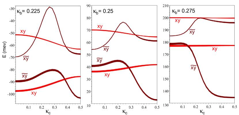
Figure 25: The two quasi-1D, metallic bands in the gap between the valence (V) and conduction (C) bands as functions of the perpendicular $k_{c}$ in the irreducible BZ, $0\leq k_{c}<0.5,$ and for $k_{b}$ fixed at 0.225, 0.250, and 0.275. The red bands are the pure $xy$ bands and the dark-red $\widetilde{xy}$ bands include the hybridization with the four V&C bands. The extra fatness (band decoration) is proportional to the $\left|\mathbf{k}\right\rangle$ character, which for the dark-red bands was obtained from the two-band Hamiltonian (121). The red and the dark-red fat bands for $k_{b}$=0.225 were already shown in respectively FIG.s I 6 and 7, and their $\left|\mathbf{k}\right\rangle$ characters in the middle and bottom parts of FIG. II 14. The upper and lower $\widetilde{xy}$ bands as functions of $\left(k_{b},k_{c}\right)$ are shown on the left-hand side of FIG. 27. The ARPES-refined TB parameter values I (43)-(46) were used and the $xz$-$yz$ hybridization [parameters I (40)] was neglected.${}^{\ref{NeglectLambda}}$ The value of $E$ in the denominators were iteratively adjusted to equal the eigenvalue in question of the two-band Hamitonian whereby it equals the appropriate eigenvalue of the six-band Hamiltonian (with the values I (47) of the $xz$-$yz$ parameters set to zero). The energy is in meV with respect to the center of the gap. The top of the valence band and the bottom of the conduction band are $\pm 2G_{1}=\mp 218$ meV and the ARPES samples had $E_{F}$=75 meV.

FIG. II 24 demonstrated that refinement of merely 7 of the over 40 LDA-TB parameters in our detailed six-band $t_{2g}$ Hamiltonian (Sect. I VI$)$ to fit the ARPES bands lying more than 0.15 eV below the Fermi level, achieves nearly perfect agreement also for the $k_{c}$-dispersion of the quasi-1D bands closer to the Fermi level. This includes agreement with the size and shape of the resonance peak in the upper band –blue in (c2)– without having modified any of the 17 $\left(a,g,\alpha,\gamma\right)$-parameters I (46) describing the hybridization between the $xy$ and the $xz\,$and $yz$ V&C bands, parameters which we shall see decisively influence the structure of the metallic $\widetilde{xy}$ bands via the second order terms (125) and (XIV.1.2) in the two-band Hamiltonian (121).

The resonance peaks are pushed $\genfrac{}{}{0.0pt}{}{\mathrm{up}}{\mathrm{down}}$ in the $\genfrac{}{}{0.0pt}{}{\mathrm{upper}}{\mathrm{lower}}$ $\widetilde{xy}$ band by the edges of $\genfrac{}{}{0.0pt}{}{\mathrm{V}}{\mathrm{C}}$-bands, whose characters before hybridization with the $xy$ band are 50% mixed $\left|xz;\mathbf{k}\right\rangle$ and $\left|xz;\mathbf{k+c}^{\ast}\right\rangle,$ or $\left|yz;\mathbf{k}\right\rangle$ and $\left|yz;\mathbf{k+c}^{\ast}\right\rangle;$ it is therefore not obvious to what extent the character (fatness) of the original $xy$ bands (the red ones in the middle panel of FIG. II 14) near $k_{c}$=$\pm$0.75 or $\pm 0.25$ are retained in the hybridized $\widetilde{xy}$ bands, and, hence, how strong the ARPES intensity should be. The selection rule that the ARPES intensity follows the $\left|\mathbf{k}\right\rangle$ character holds also for the two weakly hybridized $\widetilde{xy}$ bands, because –to lowest order– the effect of weak hybridization is to distort the bands. The $\left|\mathbf{k}\right\rangle$ character we then compute by expressing the two bands in the $\{\mathbf{k},\mathbf{k+c}^{\ast}\}$ representation and add to the diagonal elements, $\left\langle\mathbf{k}\left|H\right|\mathbf{k}\right\rangle$, of the two-band Hamiltonian a few small, equidistant energies. This produces fat bands which include the effects of weak hybridization with the V&C bands [but neglects the relatively small effects of dimerization distortion, $\eta\left(\kappa\right)$ Eq. II (78)].

We therefore need to compute the $\left|\mathbf{k}\right\rangle$ character of the $\widetilde{xy}$ bands. This we do by using the Hamiltonian (121) obtained by downfolding [87] of the V&C blocks of the six-band Hamiltonian I (56) in the $\left\{\mathbf{k,k+c}^{\ast}\right\}$-representation. For simplicity of the formalism, we neglect the mixing between the $xz$ and $yz$ WOs, which is a good approximation near the FS, $\left|k_{b}\right|\sim 0.25,$ far away from the Y and Z points (see FIG. I 8). The derivation of this two-band Hamiltonian will be our first task in the theoretical Sect. XIV of the present paper.

The two-band Hamiltonian is also the one from which we can best understand the origin of the splitting and perpendicular dispersion of the two metallic bands shown in FIG. 25, including their development with increasing $k_{b},$ which is surprisingly unsymmetric around half-filling, $k_{b}$=$0.25$. Having discussed the two bands in great detail in Sect. XIV.2 and understood that merely the light-red $xy$ –but not the dark-red $\widetilde{xy}$– bands can be described by a $2\times 2$ TB Hamiltonian, we shall in the final theoretical subsection XIV.3 present and discuss their constant-energy contours (CECs), the FS in particular.

The second part of this paper, starting from Sect. XV, is devoted to the demanding task of using ARPES to determine the FS and its velocities. First, the challenges, issues, and methods are discussed in Sect. XV.1. The results of the FS and velocity extraction are then shown in Sect. XV.2. They are compared with the TB theory using the ARPES refined parameters and are finally presented in FIG. 32.

In theory, the (fine-grained) ARPES intensity from each metallic band is periodic in the double zone ($|\kappa_{c}|\leq 1$) with the intensity from the lower band (outer sheet) dominating in the 1st zone ($|\kappa_{c}|\leq 0.5$) and the intensity from the upper band (inner sheet) dominating in the 2nd zone ($|\kappa_{c}|\geq 0.5$). Between zone centers ($\kappa_{c}$ integer), the origin of the dominating intensity thus switches from one band (sheet) to the other, with the intensities being equal at the zone boundary (see Fig. 29). Since the measured spectra of the sheets possess a finite width in momentum, which is much larger than the splitting of the sheets, we can only detect the center of gravity of the sum of intensities from the occupied bands. By taking this into account, the experimentally obtained FS fits the theoretical one very well. At the zone boundary, we determined an upper bound for the splitting, which is in that sense, in agreement with the theory, that it is larger than the theoretical value. Comparing the experimentally extracted velocities with the theoretical ones, we reach a similar perfect fit as for the FS. Interestingly, the velocities are generally greater than those for pure LDA by about 15%, as we discuss in detail in Sect. XV.2.2.

XIV Theoretical splitting and perpendicular dispersion of the two metallic bands in the gap

XIV.1 Hamiltonian for the two metallic bands in the $\left\{\mathbf{k,k+c}^{\ast}\right\}$-representation and of resonance form

We start from the six-band Hamiltonian I (56) in the $\left\{\mathbf{k,k+c}^{\ast}\right\}$-representation:

$$\framebox{{\hbox{\begin{array}[]{cccccccc}H&&\left|xy;\mathbf{k}\right\rangle&\left|xy;\mathbf{k+c}^{\ast}\right\rangle&\left|xz;\mathbf{k}\right\rangle&\left|xz;\mathbf{k+c}^{\ast}\right\rangle&\left|yz;\mathbf{k}\right\rangle&\left|yz;\mathbf{k+c}^{\ast}\right\rangle\\ &&&&&&&\\ \left\langle xy;\mathbf{k}\right|&&\tau+t&iu&\alpha+a&i\left( \gamma+g\right)&\bar{\alpha}+\bar{a}&i\left( \bar{\gamma}+\bar{g}\right)\\ \left\langle xy;\mathbf{k+c}^{\ast}\right|&&-iu&\tau-t&i\left( \gamma-g\right)&\alpha-a&i\left( \bar{\gamma}-\bar{g}\right)&\bar{\alpha}-\bar{a}\\ \left\langle xz;\mathbf{k}\right|&&\alpha+a&-i\left( \gamma-g\right)&A&iG&\lambda+l&-i\left( \mu-m\right)\\ \left\langle xz;\mathbf{k+c}^{\ast}\right|&&-i\left( \gamma+g\right)&\alpha-a&-iG&-A&-i\left( \mu+m\right)&\lambda-l\\ \left\langle yz;\mathbf{k}\right|&&\bar{\alpha}+\bar{a}&-i\left( \bar{\gamma}-\overline{g}\right)&\lambda+l&i\left( \mu+m\right)&\bar{A}&i\bar{G}\\ \left\langle yz;\mathbf{k+c}^{\ast}\right|&&-i\left( \bar{\gamma}+\bar{g}\right)&\bar{\alpha}-\bar{a}&i\left( \mu-m\right)&\lambda-l&-i\bar{G}&-\bar{A}\end{array}}}}.$$ (105)

Like in Eq. I (35), the argument, $\mathbf{k,}$ of the Bloch sums of hopping integrals I (36)-(40) is omitted for brevity and an overbar, used when switching from an $xz$ to a $yz$ orbital, indicates the mirror operation $k_{b}\leftrightarrow-k_{b}$.

XIV.1.1 Six-band Hamiltonian in the V&C subband representation

Since the largest off-diagonal elements I (43)-(47) are $\bar{G}$ and $G,$ which gap the $yz$ bands as in Eq. I (29) and the $xz$ bands in the same way, but with $k_{b}$ substituted by $-k_{b}$, we shall now turn to a representation in which the $xz$-$xz$ and $yz$-$yz$ blocks are diagonal. This mixed representation is the natural one to use for downfolding these blocks of the six-band Hamiltonian to a two-band Hamiltonian which then describes merely the two $\widetilde{xy}$ bands in the gap and –provided that we neglect the hybridization I (40) between the $xz$ and $yz$ bands– has the simple resonance form (121). As said above, this approximation of using the $\left(m,m^{\prime}\right)$-unhybridized, socalled pure $xz$ and $yz$ bands (Sect. I VI.3) is a good one far away from Y and Z, especially near the FS, $\left|k_{b}\right|\sim 0.25$ (FIG. I 8). The eigenvalues, $\pm\sqrt{\bar{A}^{2}+\bar{G}^{2}},$ of the $yz$-$yz$ 2$\times$2 diagonal block of the six-band Hamiltonian, Eq. I (56), are the $yz$ conduction (C)- and valence (V)-band energies I (29), and so are $\pm\sqrt{A^{2}+G^{2}}$ for the $xz$ $\genfrac{}{}{0.0pt}{}{C}{V}$-band energies. The structure of the six bands for $k_{b}$=0.225, 0.250, and 0.275 as a function of $k_{c}$ may be seen on the 3rd line to the left in FIG. 26 and we shall describe it in Sect. XIV.2.

The orthonormal $xz$ C&V-band orbitals are:

$$\left(\begin{array}[]{cc}\left|xz_{C}\left(\mathbf{k}\right)\right\rangle&\left|xz_{V}\left(\mathbf{k}\right)\right\rangle\end{array}\right)=\left(\begin{array}[]{cc}\left|xz;\mathbf{k}\right\rangle&\left|xz;\mathbf{k+c}^{\ast}\right\rangle\end{array}\right)\times\frac{1}{2}\left(\begin{array}[]{cc}e^{-i\phi}-1&e^{-i\phi}+1\\ e^{-i\phi}+1&e^{-i\phi}-1\end{array}\right),$$ (106)

where the $xz$ band-structure phase, $\phi\left(\mathbf{k}\right),$ is that of $-A\left(\mathbf{k}\right)-iG\left(\mathbf{k}\right).$ The $\left|\mathbf{k}\right\rangle$ $\left(=1-\left|\mathbf{k+c}^{\ast}\right\rangle\right)$ characters –or fatnesses– of the $\genfrac{}{}{0.0pt}{}{C}{V}$ bands are:

$$f_{\genfrac{}{}{0.0pt}{}{C}{V}}\left(\mathbf{k}\right)=\left|\frac{e^{-i\phi}\mp 1}{2}\right|^{2}=\frac{1\mp\cos\phi}{2},$$ (107)

and they are shown on the 3rd line to the right in FIG. 26 in $\frac{\mathrm{light}}{\mathrm{dark}}$ blue. While the (C and V) bands are periodic, their fatnesses are periodic in the double zone (see FIG. I 6).

Using the unitary matrix I (59) to transform the six-band Hamiltonian I (56) to the pure-$xz$ representation in which the V&C block is diagonal yields:

H—xy;k⟩—xy;k+c^∗⟩—xz_C(k)⟩—xz_V(k)⟩⟨xy;k—τ+tiucccc⟨xy;k+c^∗—-iuτ-tcccc⟨xz_C(k)—(α+a)eiϕ-12-i(γ+g)eiϕ+12(α-a)eiϕ+12-i(γ-g)eiϕ-12A^2+G^20⟨xz_V(k)—(α+a)eiϕ+12-i(γ+g)eiϕ-12(α-a)eiϕ-12-i(γ-g)eiϕ+120-A^2+G^2 (108)

for the first four rows and columns. The last two ($yz_{C}$ and $yz_{V})$ rows and columns obtained by transformation to the pure-$yz$ representation, equal those given above for $xz_{C}$ and $xz_{V},$ but with $k_{b}$ substituted by $-k_{b},$ or $A$ and $G$ substituted by $\bar{A}$ and $\bar{G}$.

XIV.1.2 Löwdin-downfolded two-band Hamiltonian

The WOs for the two $\widetilde{xy}$ bands in the gap have much longer range than the $xy$-WOs shown in FIG.s I 5 and I 9, and similarly for the elements in the effective two-band Hamiltonian compared with the range of the Bloch sums in the six-band Hamiltonian. For this reason, we do not perform the downfolding of the $xz,$ $XZ,$ $yz,$ and $YZ$ WOs into the ”tails” of the $\widetilde{xy}$ and $\widetilde{XY}$ WOs in real space, but in reciprocal space. Real-space pictures of these downfolded orbitals would be unwieldy and would crucially depend on the position of the energies, $E,$ of the bands in the gap. For the same reason, tables of hopping integrals would be unwieldy and energy dependent. For the downfolding from six to two narrow bands near the centre of the gap, we can use simple, analytical Löwdin[87]- rather than numerical (NMTO) downfolding because the splitting of the two $\widetilde{xy}$ bands is far less than their distance to the C&V-band edges (see the left-hand panels on the 3rd line in FIG. 26). Hence, the explicit dependence of the two-band Hamiltonian (4) on the TB parameters I (43)-(47) is preserved.

With the hybridization between the $xz$ and $yz$ orbitals neglected, the $xz$ and $yz$ downfoldings are additive:

$$\left(\begin{array}[]{ll}\left|\widetilde{xy};E,\mathbf{k}\right\rangle&\left|\widetilde{xy};E,\mathbf{k+c}^{\ast}\right\rangle\end{array}\right)=\left(\begin{array}[]{ll}\left|xy;\mathbf{k}\right\rangle&\left|xy;\mathbf{k+c}^{\ast}\right\rangle\end{array}\right)+\delta_{xz;E}\left(\begin{array}[]{ll}\left|xy;\mathbf{k}\right\rangle&\left|xy;\mathbf{k+c}^{\ast}\right\rangle\end{array}\right)+\delta_{yz;E}\left(\begin{array}[]{ll}\left|xy;\mathbf{k}\right\rangle&\left|xy;\mathbf{k+c}^{\ast}\right\rangle\end{array}\right).$$ (109)

Here, the $\delta_{xz;E}$ and $\delta_{yz;E}$ perturbations involve the Green function for the $xz$-$xz$ or $yz$-$yz$ block of the six-band Hamiltonian I (56) times the corresponding $xz$-$xy$ or $yz$-$xy$ hybridization matrix. The representation chosen for the $xz$ and $yz$ states to be downfolded (integrated out) matters for the formalism, but not for the resulting two-band Hamiltonian. Choosing the pure-$m$ representation (108) in which the $xz$-$xz$ and the $yz$-$yz$ blocks of the Hamiltonian are diagonal we get:

$$\delta_{xz;E}\left(\begin{array}[]{cc}\left|xy;\mathbf{k}\right\rangle&\left|xy;\mathbf{k+c}^{\ast}\right\rangle\end{array}\right)=$$ (111)

$$\frac{\left|xz_{C}\right\rangle}{E-\sqrt{A^{2}+G^{2}}}\left(\begin{array}[]{cc}\left\langle xz_{C}\left|H\right|xy;\mathbf{k}\right\rangle&\left\langle xz_{C}\left|H\right|xy;\mathbf{k+c}^{\ast}\right\rangle\end{array}\right)+\frac{\left|xz_{V}\right\rangle}{E+\sqrt{A^{2}+G^{2}}}\left(\begin{array}[]{cc}\left\langle xz_{V}\left|H\right|xy;\mathbf{k}\right\rangle&\left\langle xz_{V}\left|H\right|xy;\mathbf{k+c}^{\ast}\right\rangle\end{array}\right),$$ (114)

and similarly for $\delta_{yz;E}.$ It is by virtue of this choice that the $E$-dependence of the downfolded orbitals enters solely through the denominators in (111).

In the $\left\{\widetilde{xy};E,\mathbf{k,k+c}^{\ast}\right\}$-representation (109), the two-band Hamiltonian is finally seen to be:

$$\left(\begin{array}[]{cc}\left\langle\widetilde{xy};E,\mathbf{k}\left|H\right|\widetilde{xy};E,\mathbf{k}\right\rangle&\left\langle\widetilde{xy};E,\mathbf{k}\left|H\right|\widetilde{xy};E,\mathbf{k+c}^{\ast}\right\rangle\\ c.c.&\left\langle\widetilde{xy};E,\mathbf{k+c}^{\ast}\left|H\right|\widetilde{xy};E,\mathbf{k+c}^{\ast}\right\rangle\end{array}\right)=\tau\left(k_{b}\right)\left(\begin{array}[]{cc}1&0\\ 0&1\end{array}\right)+\left(\begin{array}[]{cc}t\left(\mathbf{k}\right)&iu\left(\mathbf{k}\right)\\ -iu\left(\mathbf{k}\right)&-t\left(\mathbf{k}\right)\end{array}\right)$$ (121)

$$+\frac{\Gamma_{C}\left(\mathbf{k}\right)}{E-\sqrt{A^{2}\left(\mathbf{k}\right)+G^{2}\left(\mathbf{k}\right)}}+\frac{\Gamma_{V}\left(\mathbf{k}\right)}{E+\sqrt{A^{2}\left(\mathbf{k}\right)+G^{2}\left(\mathbf{k}\right)}}+\frac{\overline{\Gamma}_{C}\left(\mathbf{k}\right)}{E-\sqrt{\bar{A}^{2}\left(\mathbf{k}\right)+\bar{G}^{2}\left(\mathbf{k}\right)}}+\frac{\overline{\Gamma}_{V}\left(\mathbf{k}\right)}{E+\sqrt{\bar{A}^{2}\left(\mathbf{k}\right)+\bar{G}^{2}\left(\mathbf{k}\right)}},$$

with the directly coupled terms on the 1st line and the resonance terms for the coupling via the C&V bands on the 2nd line. The poles at the C&V $xz$ and $yz$ bands, $\pm\sqrt{A^{2}\left(\mathbf{k}\right)+G^{2}\left(\mathbf{k}\right)}$ and $\pm\sqrt{\bar{A}^{2}\left(\mathbf{k}\right)+\bar{G}^{2}\left(\mathbf{k}\right)},$ are numbers while the residues, $\Gamma_{C}\left(\mathbf{k}\right),$ $\Gamma_{V}\left(\mathbf{k}\right)$, $\overline{\Gamma}_{C}\left(\mathbf{k}\right),$ and $\overline{\Gamma}_{V}\left(\mathbf{k}\right)$, are 2$\times$2 matrices of the following form for the perturbation by the $xz$ C band:

$$\Gamma_{C}\left(\mathbf{k}\right)=\left(\begin{array}[]{cc}\left|\left\langle xz_{C}\left(\mathbf{k}\right)\left|H\right|xy;\mathbf{k}\right\rangle\right|^{2}&\left\langle xy;\mathbf{k}\left|H\right|xz_{C}\left(\mathbf{k}\right)\right\rangle\left\langle xz_{C}\left(\mathbf{k}\right)\left|H\right|xy;\mathbf{k+c}^{\ast}\right\rangle\\ cc&\left|\left\langle xz_{C}\left(\mathbf{k}\right)\left|H\right|xy;\mathbf{k+c}^{\ast}\right\rangle\right|^{2}\end{array}\right),$$ (122)

and similarly for the perturbation by the $xz$ V band. Since translation of $\mathbf{k}$ by $\mathbf{c}^{\ast}$ yields:

$$\widehat{\mathbf{c}^{\ast}}\left\langle\mathbf{k}\left|\Gamma\right|\mathbf{k}\right\rangle=\left\langle\mathbf{k+c}^{\ast}\left|\Gamma\right|\mathbf{k+c}^{\ast}\right\rangle,$$ (123)

the two diagonal elements with $\mathbf{k}$ in the single zone reduce to one real-valued function of $\mathbf{k,}$ periodic in the double zone. For the purely imaginary off-diagonal element:

$$\widehat{\mathbf{c}^{\ast}}\left\langle\mathbf{k}\left|\Gamma\right|\mathbf{k+c}^{\ast}\right\rangle=\left\langle\mathbf{k+c}^{\ast}\left|\Gamma\right|\mathbf{k}\right\rangle=\left\langle\mathbf{k}\left|\Gamma\right|\mathbf{k+c}^{\ast}\right\rangle^{\ast}=-\left\langle\mathbf{k}\left|\Gamma\right|\mathbf{k+c}^{\ast}\right\rangle,$$ (124)

i.e. it is an anti-periodic function of $\mathbf{k}$ in the single zone.

The elements of the matrix (122) are given by those of Eq. (108) in terms of the $xz$-band phase $\phi\left(\mathbf{k}\right)$ [I (60)] and the Bloch sums of the $xy$-$xz$ intra- and inter-ribbon hopping integrals $\alpha\pm a$ and $\gamma\pm g$ $\left[\text{I}~{}\text{(39)}\right],$ and may be expressed as:

$$\left\langle\mathbf{k}\left|\Gamma_{\genfrac{}{}{0.0pt}{}{C}{V}}\left(\mathbf{k}\right)\right|\mathbf{k}\right\rangle=\left|\left\langle xz_{\genfrac{}{}{0.0pt}{}{C}{V}}\left(\mathbf{k}\right)\left|H\right|xy;\mathbf{k}\right\rangle\right|^{2}=\left[\left(\alpha+a\right)f_{\genfrac{}{}{0.0pt}{}{C}{V}}\mp\left(\gamma+g\right)\frac{\sin\phi}{2}\right]^{2}+\left[\left(\gamma+g\right)f_{\genfrac{}{}{0.0pt}{}{V}{C}}\mp\left(\alpha+a\right)\frac{\sin\phi}{2}\right]^{2}$$ (125)

for the diagonal elements, and as:

$$\left\langle\mathbf{k}\left|\Gamma_{\genfrac{}{}{0.0pt}{}{C}{V}}\left(\mathbf{k}\right)\right|\mathbf{k+c}^{\ast}\right\rangle = \left\langle xy;\mathbf{k}\left|H\right|xz_{\genfrac{}{}{0.0pt}{}{C}{V}}\left(\mathbf{k}\right)\right\rangle\left\langle xz_{\genfrac{}{}{0.0pt}{}{C}{V}}\left(\mathbf{k}\right)\left|H\right|xy;\mathbf{k+c}^{\ast}\right\rangle$$

$$= i\left[-\left(\alpha+a\right)\left(\gamma-g\right)f_{\genfrac{}{}{0.0pt}{}{C}{V}}+\left(\gamma+g\right)\left(\alpha-a\right)f_{\genfrac{}{}{0.0pt}{}{V}{C}}\pm\left(\left(\alpha+a\right)\left(\alpha-a\right)+\left(\gamma+g\right)\left(\gamma-g\right)\frac{\sin\phi}{2}\right)\right]$$

for the off-diagonal elements, which are purely imaginary. They are shown on the 4th line of FIG. 26 as functions of $k_{c}$ for $k_{b}=0.225,$ 0.250, and 0.275 and will be discussed in Sect XIV.2.5. On the 5th line, we show the $xy$-$xz$ intra and inter-ribbon hopping integrals: to the left $\alpha+a$ in purple and $\alpha-a$ in grey, and to the right $\gamma+g$ in turquise and $\gamma-g$ in grey. These Bloch sums are periodic in the double zone and each grey Bloch sum equals the colored one inside the same frame, but translated by $\mathbf{c}^{\ast}.$ This follows from Eq.s I (41) and (42). Together with the $\left|\mathbf{k}\right\rangle$ characters of the C and V bands, $f_{C}$ and $f_{V},$ in respectively light and dark blue on the 3rd line to the right, $\frac{1}{2}\sin\phi$ is shown in grey.

The residues for the perturbations by the $yz$ C&V bands are respectively $\overline{\Gamma}_{C}\left(\mathbf{k}\right)$ and $\overline{\Gamma}_{V}\left(\mathbf{k}\right)$ with the overbar indicating the mirror operation $k_{b}\leftrightarrow-k_{b}$.

$E$ is the energy of the $\widetilde{xy}$ state that we are seeking, i.e. the upper or lower eigenvalue of the two-band Hamiltonian (121), and should therefore be found self-consistently. For states deep inside the gap, we may substitute $E$ by $\tau\left(k_{b}\right)$ from Eq. I (36) because the splitting of the two $\widetilde{xy}$ bands is far less than half the gap. Note that $E$ is with respect to the center of the gap and that it enters the two-band Hamiltonian (121) only through the denominators of the four resonance terms. Keeping $E$ as a free parameter therefore provides insight to study how the perpendicular dispersion of the $\widetilde{xy}$-bands depend on their placement in the gap and on the $\mathbf{k}$-dependence of the four residues.

The simplest way to understand the energy dependence of a Löwdin-downfolded Hamiltonian, $\widetilde{H}(E),$ is to consider downfolding of a $2\times 2$ Hamiltonian, $H:$ Its exact $E$-eigenvalues are the roots of the secular determinant $\left|H-E1\right|=\left(H_{11}-E\right)\left(H_{22}-E\right)-\left|H_{12}\right|^{2},$ which satisfy: $E=H_{11}+\left|H_{12}\right|^{2}\left/(E-H_{22})\right.\equiv\widetilde{H}(E),$ showing that $\widetilde{H}(H_{11})$ is the well-known 2nd order estimate of the eigenvalue closest to $H_{11}$ and that $\widetilde{H}(E)$ has a pole at the energy, $H_{22}.$ It should now be obvious that the six-band Hamiltonian (108) can be downfolded to a two-band Hamiltonian with the form (121).

XIV.2 Origin of the splitting and perpendicular dispersion

Having derived a Hamiltonian (121) for the two metallic $\widetilde{xy}$ bands in the gap (FIG. 25) consisting of TB plus resonance terms, we now take up the thread and trace the non-trivial features of the bands back to the Bloch-sums I (36)-(37), $\tau\left(k_{b}\right),$ $t\left(\mathbf{k}\right),$ and $u\left(\mathbf{k}\right),$ of the $xy$-$xy$ hopping integrals, to the Bloch sums I (38), $A\left(k_{c}\mp k_{b}\right)$ and $G\left(k_{c}\mp k_{b}\right),$ of the $xz$-$xz$ or $yz$-$yz$ hopping integrals, and to the Bloch sums I (VI.1), $\alpha\left(\mathbf{k}\right)\pm a\left(\mathbf{k}\right)$ and $\gamma\left(\mathbf{k}\right)\pm g\left(\mathbf{k}\right),$ of the $xy$-$xz$ hopping integrals. This is a long route and the essence may be extracted from the synthesis in Sect. XIV.2.7.

We start by extending FIG. 25 from the irreducible $\left(0\leq k_{c}\leq 0.5\right)$ to the double $\left(-1<k_{c}\leq 1\right)$ zone in which all Bloch sums are periodic (the Greek- and Latin-lettered Bloch sums are periodic in respectively the single and the double zone). This is done in FIG. 26 on the top line to the right (the figure to the left will be described in the last paragraph of this subsection), in each of three panels, for $k_{b}$=0.225, 0.250 and 0.275, i.e. along the brown, red, and olive dot-dashed lines in FIG. I 8. For clarity, the color of the $\widetilde{xy}$ bands has been changed from dark-red to black in FIG. 26.

Upon increasing $k_{b}$ from 0.225 to 0.275, we see the $\widetilde{xy}$ bands develop from having strong upwards-pointing peaks in the upper band near $k_{c}$=$\pm$0.75 and $\pm$0.25, plus small downwards bulges in the lower band around $k_{c}$=$\pm$0.5, over having reduced peaks and increased bulges –and thus minimal total width– near midgap, to having large downwards-pointing peaks connected pairwise by large bulges in the lower band, plus reminiscences of the upwards-pointing peaks in the upper band. This development is far from symmetric around the mid-gap energy $(\equiv 0)$, despite the fact that the V and C bands on either side of the direct gap have the same character, apart from being respectively $xz$-$XZ$ (or $yz$-$YZ$) bonding and anti-bonding. In the present section we shall show in didactic detail that the origin lies in the complicated bi-products (122) forming the residues, $\Gamma\left(\mathbf{k}\right),$ of the matrix elements for the resonant couplings.

On lines 2-5 in Fig. 26, we identify and analyze the individual contributions from the direct $xy$-$xy$ hops (red) and the indirect hops via the $xz$ (blue) and $yz$ (green) V&C bands to the diagonal and off-diagonal elements, $\left\langle\widetilde{xy};\mathbf{k}\left|H\right|\widetilde{xy};\mathbf{k}\right\rangle$ and $\left\langle\widetilde{xy};\mathbf{k}\left|H\right|\widetilde{xy};\mathbf{k+c}^{\ast}\right\rangle,$ of the two-band Hamiltonian (121). We end on line 5 with $\alpha\left(\mathbf{k}\right)\pm a\left(\mathbf{k}\right)$ in $\genfrac{}{}{0.0pt}{}{\mathrm{purple}}{\mathrm{grey}}$ and $\gamma\left(\mathbf{k}\right)\pm g\left(\mathbf{k}\right)$ in $\genfrac{}{}{0.0pt}{}{\mathrm{turquoise}}{\mathrm{grey}}$.

For simplicity in FIG. 26, we have substituted $E$ in the denominators of the resonance terms (121) by $\tau\left(k_{b}\right)$ and shall use a notation in which we drop this argument from e.g. $\left\langle\widetilde{xy};\tau\left(k_{b}\right),\mathbf{k}\left|\,H\,\right|\widetilde{xy};\tau\left(k_{b}\right),\mathbf{k+c}^{\ast}\right\rangle.$ This approximation slightly enhances the peak features, as may be seen by comparison of FIG.s 25 and 26.

The bands –but not their $\left|\mathbf{k}\right\rangle$ decoration (extra fatness)– have the proper single-zone period $1$ in $k_{c}.$ Where one band is fat and the other not, those bands have respectively pure $\left|\mathbf{k}\right\rangle$ and pure $\left|\mathbf{k+c}^{\ast}\right\rangle$ character. This is the case for integer values of $k_{c}$, whereas for half-integer values, the two bands are of 50% mixed character.

To the left on the 1st line, we show in respectively fat and thin lines the unhybridized $\widetilde{xy}\left(\mathbf{k}\right)$ and $\widetilde{xy}\left(\mathbf{k+c}^{\ast}\right)$ bands. These are the diagonal elements, $\left\langle\widetilde{xy};\mathbf{k}\left|H\right|\widetilde{xy};\mathbf{k}\right\rangle$ and $\left\langle\widetilde{xy};\mathbf{k+c}^{\ast}\left|H\right|\widetilde{xy};\mathbf{k+c}^{\ast}\right\rangle$ of the two-band Hamiltonian (121) and have the double-zone period $2$ in $k_{c}$.

XIV.2.1 Peak-, bulge-, and contact features

The primary feature of the $\widetilde{xy}$ bands in the gap, the resonance peaks, originate from either an $xz$-band edge, which runs along a blue YZY’ line in FIG. I 8, or from a $yz$-band edge, which runs along a green YZY’ line in the same figure, and are therefore located at the crossings between such a line and the two red $\widetilde{xy}$-band CECs seen in the uppermost panels of FIG. II 20 (b). In the CECs, the resonance peaks appear as notches. With reference to the bands for fixed values of $k_{b}$ in FIG. 25, a resonance peak is located where a band edge crosses the appropriate constant $k_{b}$-line (dot-dashed in FIG. I 8). The resonance features are therefore well separated in $k_{c}$ as seen in FIG. 26 on the 1st line to the right.

From the fatnesses of the bands we see that the resonance peaks have almost pure $\left|\widetilde{xy};\mathbf{k}\right\rangle$ or $\left|\widetilde{xy};\mathbf{k+c}^{\ast}\right\rangle$ character, although the V&C-band edges have $\sim$50% mixed $\left|xz;\mathbf{k}\right\rangle$ and $\left|xz;\mathbf{k+c}^{\ast}\right\rangle$ (or $\left|yz;\mathbf{k}\right\rangle$ and $\left|yz;\mathbf{k+c}^{\ast}\right\rangle)$ characters, as we saw along $\Lambda\mathrm{W}$ ($k_{c}$=$\frac{1}{4})$ and $\Lambda^{\prime}\mathrm{W}^{\prime}$ ($k_{c}$=$\frac{3}{4})$ in FIG. II 21 (d) and (e). The strong $\left|\mathbf{k}\right\rangle$ character is what enabled us, in Sect. XI.2 of Paper II, to detect with ARPES the large peak in the upper $\widetilde{xy}$ band from the resonance with the blue $xz$ valence band at $\mathbf{k}$=$\left(0.225,0.725\right),$ mirrored (”symmetrized”) around $k_{c}$=0.5 to $\left(0.225,0.275\right)$. That the lower $\widetilde{xy}$ band merely exhibits a shoulder at $\left(0.225,0.725\right)$ will be explained later, at the beginning of Sect. XIV.2.5.

The understanding is quite different for the secondary feature, seen around the BZ boundaries $\left(k_{c}\text{=}\pm 0.5\right)$ on the 1st line in FIG. 26 to the right (but absent to the left). This feature consists of a bulge in the lower band and the concomitant filling-in of the valleys between the neighboring resonance peaks repelled by the $xz$ and $yz$ V or C bands, whichever is closer in energy. These neighboring resonance peaks are therefore in the upper $\widetilde{xy}$ band when $k_{b}$=0.225 and 0.250, and in the lower $\widetilde{xy}$ band when $k_{b}$=0.275. The bulge is caused by the hybridization between the $\widetilde{xy}\left(\mathbf{k}\right)$ and $\widetilde{xy}\left(\mathbf{k+c}^{\ast}\right)$ bands –displayed to the left– which cross at $k_{c}$=$\pm 0.5$ and split by $\pm\left|\left\langle\widetilde{xy};\mathbf{k}\left|H\right|\widetilde{xy};\mathbf{k}+\mathbf{c}^{\ast}\right\rangle\right|.$ The latter, off-diagonal matrix element of the two-band Hamiltonian (121) is shown in black on the 2nd line to the right. This element is seen to attain its largest absolute value near $k_{c}$=$\pm 0.5$ and, here, to have equal contributions from the indirect hops via the $xz$ (blue) and $yz$ (green) bands, and to be amplified by the direct $xy$-$xy$ (red) contribution. To the left, and in the same colors, are shown the diagonal element, $\left\langle\widetilde{xy};\mathbf{k}\left|H\right|\widetilde{xy};\mathbf{k}\right\rangle,$ and its three contributions.

Also the third characteristic feature of the $\widetilde{xy}$ bands, the near contact between the two bands –and in particular between their CECs [FIG. 27 (d)]– on the $\Gamma\mathrm{Y}$ and $\Gamma^{\prime}\mathrm{Y}^{\prime}$ lines ($k_{c}$=$\mathop{\mathrm{i}nteger}$), is connected with the hybridization between the $\widetilde{xy}\left(\mathbf{k}\right)$ and $\widetilde{xy}\left(\mathbf{k+c}^{\ast}\right)$ bands, albeit with its zero rather than its maximum [FIG. 26, black curve on the 2nd line to the right]. In ARPES [FIG. II  24 (c2)], as well as in previous calculations [25], an apparent crossing on the $\Gamma\mathrm{Y}$ line $\left(k_{c}\text{=}0\right)$ was noted and a TB description attempted [17]. With our improved resolution, this peculiarity is now seen [FIG. 27 (d)] as a splitting between the two CECs, which along $\Gamma\mathrm{Y}$ is anomalously small and even decreases with energy. This is in contrast to the relatively large splitting along ZC ($k_{c}=\frac{1}{2}+\mathop{\mathrm{i}nteger})$ which is caused by $\left(\mathbf{k,k+c}^{\ast}\right)$-hybridization and increases with energy. The splitting at integer $k_{c}$ is even smaller than that of the directly-coupled, red bands. This is simple to understand: First of all, the splitting, 2$t\left(\mathbf{k}\right)=$ $8\left(t_{1}\cos\pi k_{b}+t_{2}\cos 3\pi k_{b}\right),$ of the red bands decreases from 46 meV for $k_{b}$=0.225 to 24 meV for $k_{b}$=0.275. Secondly, along $\Gamma\mathrm{Y}$ ($k_{c}$=0) the pure $xy\left(\mathbf{k}\right),$ $xz\left(\mathbf{k}\right),$ and $yz\left(\mathbf{k}\right)$ bands are all bonding between ribbons while the $xy\left(\mathbf{k+c}^{\ast}\right),$ $xz\left(\mathbf{k+c}^{\ast}\right),$ and $yz\left(\mathbf{k+c}^{\ast}\right)$ bands are all anti-bonding [see FIG. I 6]. Since both $xy$ bands in the gap lie above the $xz\left(\mathbf{k}\right)$ and $yz\left(\mathbf{k}\right)$ bands, but below the $xz\left(\mathbf{k+c}^{\ast}\right)$ and $yz\left(\mathbf{k+c}^{\ast}\right)$ bands, the valence bands will push the bonding $xy\left(\mathbf{k}\right)$ band up, and the conduction bands will push the anti-bonding $xy\left(\mathbf{k+c}^{\ast}\right)$ band down in energy. Hence, the hybridization with the $xz$ and $yz$ V&C bands will diminish the separation between the $xy$ bands.

It is remarkable that in a region around $k_{c}$=integer, the lower $\widetilde{xy}$ band runs parallel with the red $xy$ band, and that the $k_{c}$-region over which this happens, as well as the distance above the $xy$ band, decreases with increasing $k_{b}$.

We emphasize that neither of the three characteristic features of the two metallic bands in the gap can be described by merely a 2$\times$2 TB Hamiltonian, but need the resonance terms. The three characteristic features are seen as functions of $\left(k_{b},k_{c}\right)$ on the left-hand side of FIG. 27 in Sect. XIV.3 to which we shall return.

XIV.2.2 Directly coupled terms

We now systematically identify the different terms of the two-band Hamiltonian (121).

Its first term, the energy $\tau\left(k_{b}\right)$ of the two degenerate 1D intra-ribbon $xy$ bands, is included only on the 1st line of FIG. 26, where it is the average of the two red, directly-coupled $xy$ bands, $xy\left(\mathbf{k}\right)$ and $xy\left(\mathbf{k+c}^{\ast}\right)$ to the left, or of the $\left(\mathbf{k,k+c}^{\ast}\right)$-hybridized bands to the right. This average is independent of $k_{c}.$ On the 2nd line to the left, $\tau\left(k_{b}\right)$ is neither included in the red, directly-coupled $xy\left(\mathbf{k}\right)$ band, nor in the black, directly plus indirectly-coupled $\widetilde{xy}\left(\mathbf{k}\right)$ band.

The second term in Eq. (121) is the $xy$-block of the six-band Hamiltonian I (56) and it gives the perpendicular dispersions and splitting of the red $xy$ bands shown on the 1st line in FIG. 26. The corresponding diagonal and off-diagonal matrix elements, $t\left(\mathbf{k}\right)$ and $iu\left(\mathbf{k}\right),$ are the Bloch sums of respectively the average $xy$-$XY$ hoppings and their dimerizations. They are given in Eq. I (37) and are shown in red on the 2nd line to respectively the left and the right. These Bloch sums of direct hoppings are seen to depend little on $k_{b}$ in the $\pm 10\%$ interval around $k_{F}.$

Also the TB model [17] upon which current TLL theories [5][10] are based, includes 1st- and 2nd-nearest-neighbor terms. But in the attempt to fit the peak, bulk, and band-crossing features of the LDA FS [25] without recognizing their resonant nature, the resulting TB model had an unphysical form (containing e.g. $\sin\pi k_{c}$ and $\sin 2\pi k_{c}$ terms) and, as a consequence, its parameter values are incompatible with ours. That the magnitude of its FS warping is several times ours is partly because the stoichiometry was taken to be Li_0.90 rather than Li${}_{1.02}.$

XIV.2.3 Symmetries

The red, directly-coupled and the black, directly plus indirectly-coupled $\left|\mathbf{k}\right\rangle$ bands shown to the left on the 2nd line are even around $k_{c}$=$\mathop{\mathrm{i}nteger}$. The red and black matrix elements shown to the right couple each of these bands to itself after a translation of $k_{c}$ by $1.$ These off-diagonal elements, divided by $i,$ are odd around $k_{c}$=$\mathop{\mathrm{i}nteger}$ and even around $k_{c}$=$\pm$0.5. The indirect couplings alone, i.e. the perturbations of the $\widetilde{xy}$-band Hamiltonian by the $xz$ or $yz$ V&C bands, are shown in respectively blue and green. They are related to each other by a sign change${}^{\text{II\thinspace\ref{inversion}}}$ of $k_{b}$, and those blue and red curves to the left/right are related to each other by a mirror/anti-mirror operation around $k_{c}$=$\mathop{\mathrm{i}nteger}.$ Moreover, each of the blue and green curves to the right change sign upon $k_{c}$-translation by 1, i.e. they are anti-periodic, Eq. (124).

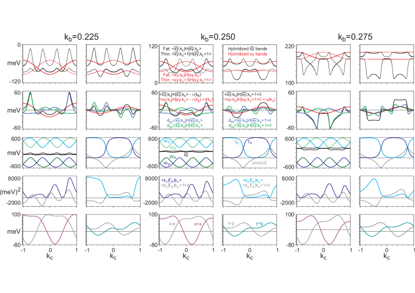
Figure 26: The following caption is for each of the three $k_{b}$-panels: 1st line: The two metallic $xy$ (red) and $\widetilde{xy}$ (black) bands, decorated with their $\left|\mathbf{k}\right\rangle$ character, as fct.s of $k_{c}$ in the double zone. $\left(\mathbf{k,k+c}^{\ast}\right)$-unhybridized (left) and -hybridized (right). The latter are as in FIG. 25, but extended to the double zone. As functions of $\left(k_{b},k_{c}\right),$ the six bands were shown on a 2 eV scale in FIG. I 4 and the two metallic bands are shown on a 0.3 eV scale in FIG. 27 (a)-(c). The 2nd line: Diagonal, $\left\langle\widetilde{xy};\mathbf{k}\left|H\right|\widetilde{xy};\mathbf{k}\right\rangle-\tau\left(k_{b}\right)$ (left), and off-diagonal, $\left\langle\widetilde{xy};\mathbf{k}\left|H\right|\widetilde{xy};\mathbf{k+c}^{\ast}\right\rangle/i$ (right), elements of the two-band Hamiltonian (121). In black, the sum of the contributions from the direct, inter-ribbon $xy$-$XY$ hops (red) and from the indirect hops via the $xz$ (blue) and $yz$ (green) valence (V) and conduction (C) bands. [Not shown are the $xy\left(\mathbf{k+c}^{\ast}\right)$ and $\widetilde{xy}\left(\mathbf{k+c}^{\ast}\right)$ bands minus $\tau\left(k_{b}\right)$ in thin black]. 3rd line left: The black $\widetilde{xy}$ bands in the gap between the blue $xz$ and green $yz$ V (dark) and C (light) bands; the hybridizations of the two latter with the $xy$ bands were neglected, i.e. $\varepsilon_{xz}$=$\mp\sqrt{A^{2}+G^{2}},$ but not vice versa. 3rd line right: $\QTATOP{\mathrm{Light}}{\mathrm{Dark}}$blue: the probability that at $\mathbf{k,}$ the $\left|xz;\mathbf{k}\right\rangle$ character is in the $\genfrac{}{}{0.0pt}{}{\mathrm{C}}{\mathrm{V}}$ band is $f_{\genfrac{}{}{0.0pt}{}{\mathrm{C}}{\mathrm{V}}}\equiv\left(1\mp\cos\phi\right)/2$ Eq. I (61). Grey: $\left(\sin\phi\right)/2.$ 4th line: Diagonal (blue) and off-diagonal (grey) matrix elements, (125) and (XIV.1.2), in meV² of the residue for the perturbation of the two-band Hamiltonian via the $xz$ V band (left) or C band (right). 5th line left: Bloch sums of $xy$-$xz$ hopping integrals I (VI.1): $\alpha+a\mathbf{\ }$(purple), $\alpha-a$ (grey); right: $\gamma+g$ (turquoise), $\gamma-g$ (grey). These four Bloch sums are periodic in the double zone and each grey Bloch sum equals the colored one inside the same frame, but translated by $\mathbf{c}^{\ast}.$ Energies are in meV with respect to the centre of the gap. The ARPES-refined parameter values were used. $E$ in the resonance terms was approximated by $\tau\left(k_{b}\right).$ See Sects. I VI and III XIV.1.

XIV.2.4 Indirectly coupled terms; role of the denominators

The indirect couplings via the $xz$ and $yz$ bands are additive and given by respectively the 3rd&4th and the 5th&6th terms in expression (121), provided that the hybridization between the $xz$ and $yz$ bands is neglected.${}^{\ref{NeglectLambda}}$ The perturbations via the $xz$ and $yz$ bands have been subdivided into V and C bands whereby each of them takes the form of a single resonance (pole) with the denominator being the distance between the narrow $\widetilde{xy}$ band and one of the four $xz$ or $yz$ V or C bands. The energy of the former is $E$ $\left[\sim\tau\left(k_{b}\right)\right],$ the energy of an $yz$ band is given by expression I (29), and that of an $xz$ band by the same expression with $k_{b}$ substituted by $-k_{b}.$ While each denominator is a single-periodic, scalar function of k, each nominator (residue) is a double-periodic 2$\times$2 matrix function given by Eq.s (122)-(XIV.1.2).

From now on, we shall take advantage of the mirror/anti-mirror symmetries mentioned in the previous Sect. XIV.2.3 between the blue $xz$- and the green $yz$ perturbations of the two-band Hamiltonian to consider merely the blue $xz$ perturbation, which we shall trace back from the 2nd line in FIG. 26 to the Bloch sums $A$ and $G$ (of respectively the symmetric and asymmetric $xz$-$xz$ integrals for hopping in- and out-side a bi-ribbon) giving the $xz$ C&V-band energies to the left and their characters, $f_{C}$ to the right on the 3rd line, and to the Bloch sums of the integrals for hopping between the $xy$ and $xz$ WOs on the 5th line.

The most important factor influencing the shapes of the diagonal and off-diagonal matrix elements shown in blue on the 2nd line to the left and the right, and given by the 3rd&4th terms in Eq. (121), is their common energy denominator. This is the distance seen on the 3rd line to the left between the $\widetilde{xy}$ bands in black and the $xz$ V or C bands in respectively dark and light blue. Also shown are the $yz$ V and C bands in respectively dark and light green. The edges, $\mp 2\left|G_{1}\right|,$ of the $xz$ bands (blue in FIG. I 8) are along $k_{c}=$ $k_{b}\mp\frac{1}{2}+2n,$ which for the three chosen values of $k_{b},$ and for $k_{c}$ in the $\left(-1|1\right)$ double-zone are at $k_{c}\sim-$0.25 and 0.75. This is where the $xz$-band edges may cause resonance peaks in the $\widetilde{xy}$ bands. The $\left|\mathbf{k}\right\rangle$ characters of the $xz$ Vand C bands, $f_{V}$ and $f_{C},$ are given by respectively the dark- and light-blue curves to the right on the 3rd line in FIG. 26.

When $k_{b}$=0.225, there is a large peak in the $\left|\mathbf{k+c}^{\ast}\right\rangle$-unhybridized $\widetilde{xy}\left(\mathbf{k}\right)$ band on the 1st line to the left near 0.75 and a small one near $-$0.25. On the 2nd line, both peaks are blue and point upwards, i.e. are caused by repulsion from the $xz$ valence band. Their sizes decrease strongly as –with $k_{b}$ increasing$-$ the $\widetilde{xy}$ bands move upwards, away from the valence band. For $k_{b}$=0.250, the peaks can still be seen in the unhybridized $\widetilde{xy}\left(\mathbf{k}\right)$ bands, as well as in the fully hybridized $\widetilde{xy}$ band on the 1st line to the right. But for $k_{b}$=0.275, when the upper $\widetilde{xy}$ band is touching the bottom of the C-band edge, only the peak from the $xz$ V-band resonance near 0.75 has survived. The small peak near $-$0.25 has been overpowered by a large, downwards pointing C-band resonance, shaped like a canine tooth. Going back to $k_{b}$=0.250, this tooth is reduced to a ”hole” on the low-$k_{c}$ side of the small, blue V-band peak near $k_{c}$=$-$0.25.

The contribution from the $xz$ V&C bands to the hybridization between the $\widetilde{xy}\left(\mathbf{k}\right)$ and $\widetilde{xy}\left(\mathbf{k+c}^{\ast}\right)$ bands is shown in blue (and divided by $i)$ on the 2nd line to the right. Whereas the diagonal element (125) of the residue matrix (122) is never negative, its $\left(\mathbf{k,k+c}^{\ast}\right)$-mixing off-diagonal elements (XIV.1.2) are purely imaginary and anti-periodic, i.e. they change sign upon translation of $k_{c}$ by 1. For $k_{b}$=0.225 the blue peak pointing downwards near 0.75 is similar to that of the diagonal element pointing upwards, but its magnitude is reduced by roughly a factor 2. For $k_{b}$ increasing, this peak decreases further and it gets superposed by the growing, anti-periodic canine-tooth structure. At the zone boundaries (ZB), $k_{c}$=$\pm$0.5, the $\widetilde{xy}\left(\mathbf{k}\right)$ and $\widetilde{xy}\left(\mathbf{k+c}^{\ast}\right)$ bands are degenerate, but get split by $\pm$ the numerical value of the off-diagonal element of the two-band Hamiltonian (121), which is seen to increase strongly with $k_{b}$. The reason is –as we shall see below– that the contribution from the V band nearly vanishes at the zone boundaries. The uncompensated repulsion from the C band is then what causes the development of the bulge in the lower $\widetilde{xy}$ band.

The V band thus causes peaks in the upper $\widetilde{xy}$ band, and the C band causes merging canine teeth plus ZB-centered bulges in the lower $\widetilde{xy}$ band. The peaks and the teeth are resonance features occurring where the FS, $\left|k_{b}\right|\sim\frac{1}{4},$ crosses between the edges, $\left|k_{c}\pm k_{b}\right|$=$\frac{1}{2},$ of $xz$ and $yz$-like V&C bands.

XIV.2.5 Indirectly coupled terms; role of the residues

The sign of a resonance term is that of its denominator, i.e. it is repulsive. As a consequence, if the Hamiltonian minus $\tau\left(k_{b}\right)$ is dominated by one of the resonance terms, e.g. due to a small denominator, that term will repel one of the two $xy$ bands, and leave the other band unperturbed. Examples are seen on the 1st line to the right in FIG. 26: Where a resonance peak exists in one of the $\widetilde{xy}$ bands, there is merely a tiny peak or shoulder in the other band. Taking, first, the resonance peak as the one caused by the blue $xz$ valence band near $k_{c}$=0.75 for $k_{b}$=0.225 or 0.250, the resonance terms parts relevant for the blue $\delta_{xz}$-perturbation on the 2nd line to the left, $\frac{\left\langle\mathbf{k}\left|\Gamma_{V}\right|\mathbf{k}\right\rangle}{\tau\left(k_{b}\right)+\sqrt{A^{2}\left(\mathbf{k}\right)+G^{2}\left(\mathbf{k}\right)}}$ and $\frac{\left\langle\mathbf{k}+c^{\ast}\left|\Gamma_{V}\right|\mathbf{k}+c^{\ast}\right\rangle}{\tau\left(k_{b}\right)+\sqrt{A^{2}\left(\mathbf{k}\right)+G^{2}\left(\mathbf{k}\right)}},$ are those near $k_{c}$=0.75 and –0.25. The closeness of the black and blue curves confirms that the Hamiltonian is, in fact, dominated by this one resonance term. Next, we go to $k_{b}$=0.275 where the $\widetilde{xy}$ bands are located just below the bottom of the C bands. The peak in the upper band caused by the repulsion from the V-band edge can still be seen on the top line to the right near $k_{c}$=0.75, but the nearby C-band edge repels the lower band much further. In fact, it is now the upper band which is the flatter and has an energy near the upper red, pure $xy$ band. The closeness of the black and blue curves on the 2nd line to the left confirms that the Hamiltonian is dominated by the $xz$-band resonances, with a minor, peak-shaped contribution from the V band near $k_{c}$=0.75 and a major, contribution with the shape of a canine tooth from the C band near $k_{c}$=–0.25. This behavior is also clearly seen in the band structures, FIG.s II 22 and 24, along the $\mathrm{ZY}$ and $\mathrm{W\Lambda}$ lines as was described in Sect. II XI. This could be another reason for the ”non-linearity” seen in FIG. 31.

The residues $\Gamma\left(\mathbf{k}\right)$ of the 4 resonance terms in expression (121) are 2$\times$2 matrices (122) with diagonal elements forming a real-valued, non-negative function of $\mathbf{k}$ which is periodic in the double zone (123) and imaginary off-diagonal elements forming an anti-periodic function of $\mathbf{k}$ in the single zone (124). These properties are clearly exhibited by the plots of expressions (125) and (XIV.1.2) on the 4th line of FIG. 26 showing $\Gamma_{C}\left(\mathbf{k}\right)$ on the right-hand sides with the diagonal element $\left\langle\mathbf{k}\left|\Gamma_{C}\right|\mathbf{k}\right\rangle$ in light blue and the off-diagonal element $\left\langle\mathbf{k}\left|\Gamma_{C}\right|\mathbf{k+c}^{\ast}\right\rangle/i$ in grey. Similarly on the left-hand sides: $\Gamma_{V}\left(\mathbf{k}\right)$ with the diagonal element $\left\langle\mathbf{k}\left|\Gamma_{V}\right|\mathbf{k}\right\rangle$ in dark blue and the off-diagonal element $\left\langle\mathbf{k}\left|\Gamma_{V}\right|\mathbf{k+c}^{\ast}\right\rangle/i$ in grey. Whereas the light blue conduction band residue follows $\left|\mathbf{k}\right\rangle$ character of the conduction band, $f_{C}$ (3rd line to the right), as expected, the dark blue valence band residue drops to zero near $k_{c}$=0.5, which is in the middle of the region where the $\left|\mathbf{k}\right\rangle$ character of the valence band dominates, and the same happens near $-0.1$. Expression (125) together with the plots of $\alpha\pm a$ and $\gamma\pm g$ on the 5th line show that the reason for the unexpected behavior of $\Gamma_{V}$ is the u-shape with two zeroes of $\alpha\left(\mathbf{k}\right)+a\left(\mathbf{k}\right).$ The zero of $\Gamma_{V}$ near $-0.85$ is caused by the zero of $\gamma\left(\mathbf{k}\right)+g\left(\mathbf{k}\right)$ shown in turquoise on the bottom line to the right.

The peaks due to resonances with the $xz$ bands occur near the $xz$-band edges. Exactly at the edges, $f_{C}$=$f_{V}$=$\frac{1}{2}$ and $\sin\phi=\pm 1.$ The $\mathbf{k}$-conserving part of the residues therefore takes the values:

$$\left\langle\mathbf{k}\left|\Gamma_{\genfrac{}{}{0.0pt}{}{\mathrm{C}}{\mathrm{V}}}\right|\mathbf{k}\right\rangle=\frac{1}{2}\left[\left(\alpha+a\right)\pm\left(\gamma+g\right)\sin\phi\right]^{2}.$$ (127)

The magnitudes and signs of $\alpha+\alpha$ and $\gamma+g$ shown in respectively purple and turquoise on the 5th line, cause the $\Gamma_{V}$ coupling at the $k_{c}$=0.75 edge (where $\sin\phi$=$-1)$ and the $\Gamma_{C}$ coupling at the $k_{c}$=–0.25 edge (where $\sin\phi$=1) to be much stronger than the two others, i.e. than the $\Gamma_{V}$ coupling at –0.25 and the $\Gamma_{C}$ coupling at 0.75, which even has a ”hole” here. This is exactly the behavior of the blue peaks seen on the 2nd line to the left.

We finally come to the grey, off-diagonal elements, $\left\langle\mathbf{k}\left|\Gamma\right|\mathbf{k+c}^{\ast}\right\rangle,$ on the 4th line. They are –roughly speaking– anti-periodic (124) versions of the double-periodic blue, diagonal elements. The reason why the grey $\left\langle\mathbf{k}\left|\Gamma_{V}\right|\mathbf{k+c}^{\ast}\right\rangle$ to the left is far more wiggly than the grey $\left\langle\mathbf{k}\left|\Gamma_{C}\right|\mathbf{k+c}^{\ast}\right\rangle$ to the right, is that not only does the former possess the two ”extra” zeroes from $\alpha+a$ near $-0.1$ and $0.5,$ as well as the one from $\gamma+g$ at $-0.85,$ but also those translated by $1$, i.e. those near $-0.5,$ $0.9,$ and $0.15.$

These very different $k_{c}$-dependencies seen on the 4th line of the blue $\left\langle\mathbf{k}\left|\Gamma_{C}\right|\mathbf{k}\right\rangle$ and $\left\langle\mathbf{k}\left|\Gamma_{V}\right|\mathbf{k}\right\rangle$ curves, and of the grey $\left\langle\mathbf{k}\left|\Gamma_{C}\right|\mathbf{k+c}^{\ast}\right\rangle$ and $\left\langle\mathbf{k}\left|\Gamma_{V}\right|\mathbf{k+c}^{\ast}\right\rangle$ curves, i.e. of the conduction- and valence-band residues, are the causes of the strong asymmetry of the perpendicular dispersion and splitting of the metallic bands around the center of the gap.

XIV.2.6 $xy$-$xz$ and $xy$-$yz$ hopping integrals

The purple $\alpha\pm a$ and turquoise $\gamma\pm g$ Bloch sums I (VI.1) shown on the bottom line are determined by the hopping integrals, $a_{n},$ $g_{n},$ $\alpha_{n},$ and $\gamma_{n},$ computed as matrix elements I (9) of the LDA Hamiltonian between $n$th-nearest-neighbor $xy$ and $xz$ (or $XZ)$ WOs (see FIG. I 9) with the results given in Table I (46). Specifically, the integrals for hopping between $xy$ and $XZ$ WOs on different sublattices are $a_{n}\pm g_{n}.$ Here, $a_{1}$ is the average of- and $g_{1}$ half the difference between the integrals for hopping from $xy$ at the origin to $XZ$ on the neigboring ribbon, inside or outside the same bi-ribbon, i.e. to $XZ$ at respectively $-0.012\mathbf{a}-0.5\mathbf{b+}0.467\mathbf{c}$ and $-\left(0.012\mathbf{a-}0.5\mathbf{\mathbf{b+}}0.533\mathbf{c}\right)$; similarly for $a_{1}^{\prime}$ and $g_{1}^{\prime},$ except that the $XZ$ orbital is translated by $\mathbf{b}$. For $a_{2}$ and $g_{2},$ the $XZ$ WO is translated by $-2\mathbf{b,}$ and for $a_{2}^{\prime}$ and $g_{2}^{\prime},$ by $2\mathbf{b.}$ For the Greek-lettered hopping integrals, the two orbitals are on the same sublattice. Specifically, the integrals for hopping from $xy$ at the origin to $xz$ at $\pm\mathbf{b}$ are $\alpha_{1}\pm\gamma_{1},$ to $xz$ at $\pm\mathbf{c}$ are $\alpha_{2}\pm\gamma_{2},$ to $xz$ at $\pm\left(\mathbf{c+b}\right)$ are $\alpha_{3}\pm\gamma_{3},$ and to $xz$ at $\mathbf{\pm}\left(\mathbf{c-b}\right)$ are $\alpha_{3}^{\prime}\pm\gamma_{3}^{\prime}.$ Calling $\gamma$ an electronic dimerization is really a misnomer, because the reason for its existence is simply the difference of relative orientation of the two orbitals. Finally, $\alpha_{0}$ is the $xy$-$xz$ on-site (crystal-field) term.

The parameters dominating the behavior of the $\alpha+a$ Bloch sum are: the integral for hopping between the $xy$ and $XZ$ nearest-neighbor WOs, $a_{1}$=$-$49 meV, and the crystal-field term, $\alpha_{0}$=31 meV. Had the former been the only non-vanishing parameter in the $\alpha+a$ Bloch sum, the corresponding term, $2a_{1}\cos\pi\left(k_{c}-k_{b}\right),$ would have killed the peak from the valence-band resonance at $\left|k_{c}-k_{b}\right|\mathrm{=}\frac{1}{2}.$ So, clearly, this peak –convincingly observed with ARPES– is sensitive to the value of the crystal-field term caused by the ribbon-inversion (see Sect. I III.1) and to the details of the $xy$-$XZ$ and $xy$-$xz$ hoppings. Note that none of these parameter values were adjusted to fit the ARPES.

XIV.2.7 Synthesis

From the bottom three lines in FIG. 26 we have seen that the $k_{c}$-dependencies of the $A,$ $G,$ $\alpha+a,$ and $\gamma+g$ Bloch sums of the $xz$-$xz$ and $xy$-$xz$ hopping integrals change relatively little for $k_{b}$ in the $\pm 10\%$ range around $k_{F}$=$\frac{1}{4}.$

By far the strongest $k_{b}$-variation of the black $\widetilde{xy}$ bands displayed on the top two lines is the one coming from the denominators of the four resonance terms via $E\approx\tau\left(k_{b}\right),$ to be seen on the 3rd line to the left, in combination with the very different shapes of the V- and C-band residues seen on the 4th line to respectively the left and the right.

What makes the blue resonance peak caused by the edge of the $xz$ V band –seen on the 2nd line to the left near $k_{c}$=0.75– differ in shape from the (unhybridized) blue canine-tooth resonance near $k_{c}$=–0.25 caused by the edge of the $xz$ C band, is the zero of the purple $\alpha+a$ near $k_{c}$=0.5 seen on the bottom line. This zero is a bit inside the frame of the dark blue $f_{V}$ window $\left(-0.25|0.75\right)$ and therefore ”cuts a hole” in $\Gamma_{V}$ on the low-$k_{c}$ side of the resonance, which is thereby sharpened up. Nothing like this happens for $\Gamma_{C}$ near $k_{c}$=–0.25, because the zero of $\alpha+a$ near –0.1 is outside the $f_{C}$ window $\left(-1.25|-0.25\right)$. Hence, it is the shape of the canine tooth which is the simpler!

On the other hand, as seen for $k_{b}$=0.275 on the 1st line to the left, the backside of the tooth at $k_{c}$=–0.25 reaches across the ZB at –0.5, where it is crossed symmetrically by the backside of the $\widetilde{xy}\left(\mathbf{k+c}^{\ast}\right)$-band tooth caused by the resonance with the $yz$ C band at $-$0.75. To the right and in black, we now see that strong $\left(\mathbf{k,k+c}^{\ast}\right)$-hybridization around $-$0.5 merges the canine teeth in the lower band at $-0.75$ and $-$0.25, thus resulting in a 60-meV splitting of the two $\widetilde{xy}$ bands.

We can go back and compare with what happens for $k_{b}$=0.225. Here, we see on the 2nd line to the left that the blue resonance peak at 0.75 is so sharp, that it hardly reaches the ZB at 0.5 and therefore hardly overlaps the peak at 0.25 in the $\widetilde{xy}\left(\mathbf{k+c}^{\ast}\right)$ band (seen above on the 1st line) from the $yz$ valence band. Moreover, the hybridization at the zone boundary ZB is much weaker than for $k_{b}$=0.275 (black curves to the right on the 2nd line) so that it merely leads to the formation of a bulge in the lower band, 35 meV below the minimum in the upper band between its resonance peaks (1st line to the right).

The zero of the purple $\alpha+a$ near $k_{c}$=0.5 which sharpens the peaks from the V bands, also makes the V bands (dark blue and dark green on line 3) contribute nothing to the $\left(\mathbf{k,k+c}^{\ast}\right)$-hybridization at the ZB. The hybridization, therefore, comes exclusively from the C bands and from the dimerization, $u,$ of the direct, perpendicular hops (red curves to the right on the 2nd line). The blue and the green –equally large– contributions each have a residue given by the value at $k_{c}$=0.5 of the grey curve to the right on line 4. For $k_{b}$ increasing from 0.225 to 0.275, this value increases from 2500 to 3500 meV² and thereby enhances the dominating effect of the decreasing denominator.

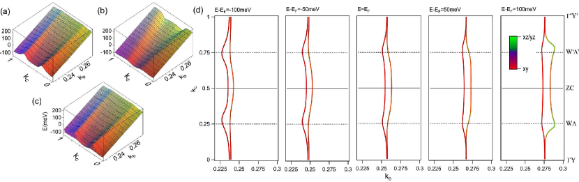
Figure 27: (a)-(c): The two $\widetilde{xy}$ quasi-1D bands in the gap for the six-band Hamiltonian I (56) with the ARPES-refined parameter values I (43)-(47). The $\mathbf{k}$-space region considered is the stripe $\pm 10\%$ around $k_{Fb}$ in the upper half of the 1st and the lower half of the 2nd BZ, $0\leq k_{c}\leq 1.$ The energies of the upper (a), the lower (b), and both metallic bands (c), relative to the center of the gap, defined as $0.$ $E_{F}$=75 meV above the center. (d): CECs calculated by tracing the roots of the secular determinant $\left|H\left(k_{a},k_{b}\right)-E\right|.$ The colors indicate the orbital characters of the bands. The notches in the inner sheet point to $\mathrm{Z}$ and those in the outer sheet to $\mathrm{Y}$ and $\mathrm{Y}^{\prime}$ (see FIG.s 11 and 20 in Paper II). The CECs have been compressed by a factor 3.3 along $k_{c}$ in order to make their warping visible. The ratio between the warping $\delta k_{\genfrac{}{}{0.0pt}{}{i}{o}Fb}$ of each (inner or outer) FS sheet and $k_{Fb}\sim 0.25$ is $\sim$0.02. This is $\sim$5 times more than without the resonant coupling to the V&C bands (see red bands for $k_{b}$=0.25 in FIG.s 25 and 26).

Finally, we shall explain why around $k_{c}$=0 the lower band is so flat, more than the upper band, and why with increasing $k_{b}$ this flatness increases and its range decreases.

But first, we will explain why the repulsion of the upper $\widetilde{xy}$ band by the C band increases far less with $k_{b}$ than expected from the decrease of the denominators (3rd line, left). The reason is found on lines 4 and 5: For the upper band near $k_{c}$=0 –which is the $\widetilde{xy}\left(\mathbf{k+c}^{\ast}\right)$ band and, hence, the $\widetilde{xy}\left(\mathbf{k}\right)$ band near $\pm$1– the light-blue C-band residue, $\Gamma_{C}\left(k_{b},~{}k_{c}\sim\pm 1\right),$ decreases by a factor 4 for $k_{b}$ increasing from 0.225 to 0.275, mainly because $\alpha+a$ decreases by almost a factor 2. This trend is furthermore enhanced by a non-vanishing repulsion from the V band whose dark-blue residue near $k_{c}$=$\pm$1 hardly changes with $k_{b}$ and thus becomes more important when $\Gamma_{C}\left(k_{b},\pm\text{1}\right)$ is small.

The reason why around $k_{c}$=0 the black lower $\widetilde{xy}$ band runs parallel to the red $xy$ band is (see line 2 to the left) that the repulsions from the blue $xz$ and the green $yz$ V bands disperse in opposite directions away from $k_{c}$=0, whereby their effects on the dispersion cancel. The reason why the distance of the black band above the red band as well as the $k_{c}$-extent of its flat part decreases with increasing $k_{b},$ is the same as the reason why the blue resonance peak near $k_{c}$=$-$0.25 is much smaller than the one near 0.75, namely: that for the dark-blue V-band residues on the 4th line $\Gamma_{V}\left(k_{b},-0.25\right)$ is much less than $\Gamma_{V}\left(k_{b},0.75\right),$ and this –in itself– is because the zero of $\alpha+a$ at $k_{c}$=$-$0.1 is closer to $-0.25$ than the zero at 0.5 is to 0.75 (purple curves on line 5). As we now –with $k_{b}$ increasing– move up in the metallic bands, the V-band perturbation decreases due to the increasing energy denominator and –as the C band is approached– canine teeth growing near $k_{c}$=$-$0.25 and 0.25 limit the region over which the lower band is flat.

We conclude that the remarkable asymmetry between the contributions from the V&C bands to the $k_{c}$-dispersion and splitting of the $\widetilde{xy}$ bands in the gap, is mainly due to the difference between the positions of the V&C bands with respect to the structure in the $\mathbf{k}$-conserving $\alpha+a$ Bloch sum of the $xy$-$xz$ hopping integrals. Specifically, the zero of $\alpha+a$ near $k_{c}$=0.5 is inside the region where the V band is formed by the $xz\left(\mathbf{k}\right)$ band –and the C band by the $xz\left(\mathbf{k+c}^{\ast}\right)$ band (see see dark- and light-blue curves in the figures to the right on line 3)– and not the other way around.

XIV.3 Constant energy contours

On the left-hand side of FIG. 27, we show the upper (a), the lower (b), and both (c) metallic $\widetilde{xy}$ bands in the gap, which extends from $-$218 meV to $+$218 meV, as functions of $\left(k_{b},k_{c}\right)$ in the stripe $0.225\leq k_{b}\leq 0.275$ and $0\leq k_{c}\leq 1.$ From the description at the beginning of Sect. XIV.2, we recognize the development of the bands –for $k_{b}$ increasing– from having strong, upwards-pointing resonance peaks near $k_{c}$=0.75 and 0.25 in the upper band (a), plus a small downwards bulge around $k_{c}$=0.5 in the lower band (b), over having reduced peaks plus a wider and deeper bulge –and minimal width– near midgap, to having strong, downwards-pointing resonance peaks (canine teeth) connected by a large bulge in the lower band, plus reminiscences of the upwards-pointing resonance peaks in the upper band. The splitting between the two bands (c) is smallest at $k_{c}$=integer where the $\left|\mathbf{k}\right\rangle$ and $\left|\mathbf{k+c}^{\ast}\right\rangle$ characters cannot mix and where the direct and indirect hoppings work in opposite directions.

In (d), we show the constant energy contours (CECs) for $k_{b}$ positive and energies ranging from 100 meV below– to 100 meV above the Fermi level which is, itself, 75 meV above the center of the gap. For $E-E_{F}$=$-$100 meV, we recognize from the LDA-TB part of FIG. II 20 , two notches pointing towards $\mathrm{Z}$ in the inner sheet and, in the outer sheet, a bulge centered at the ZB, $k_{c}$=0.5. As the energy increases, so does the distance between the bulge and the inner sheet, the notches shrink, and new notches develop in the outer sheet, on either side of the bulge, and pointing towards $\mathrm{Y}$ and $\mathrm{Y}^{\prime}\mathrm{.}$ It is obviously the resonance peaks pointing $\genfrac{}{}{0.0pt}{}{\mathrm{upwards}}{\mathrm{downwards}}$ in the $\genfrac{}{}{0.0pt}{}{\mathrm{upper}}{\mathrm{lower}}$ band which give rise to the notches pointing towards $\genfrac{}{}{0.0pt}{}{\mathrm{Z}}{\mathrm{Y}\&\mathrm{Y}^{\prime}}$ in the $\genfrac{}{}{0.0pt}{}{\mathrm{inner}}{\mathrm{outer}}$ sheets. Along $\Gamma\mathrm{Y}$ ($k_{c}$=integer), the two sheets are in near contact.

Since the quasi-1D bands disperse far more along $k_{b}$ than along $k_{c},$ the shape of two CECs in (d) resembles that of the two energy bands in FIG. 25 or in FIG. 26 on the 1st line, to the right. The $E\leftrightarrow k_{b}$ scaling is approximately: $dE=-\tau^{\prime}\left(k_{b}\right)dk_{b},$ with $\tau^{\prime}\left(k_{b}\right)$ being the dominating part of the Fermi velocity (I VI.1). This resemblance is less good close to the edge of the C- or the V-band where the hybridization with the edge makes the two bands and the two CECs behave differently: Whereas one band remains undistorted, the other gets repelled and, eventually, fuses with the CECs of the edge [see FIG. II 20].

If we interpret a CEC as a doped FS, an energy increase of 50 meV corresponds to a 4% increase of the electron doping, and the undoped FS is the CEC whose $k_{b}$ averaged over $k_{c}$ equals $\frac{1}{4}$.

We shall now analyze the ARPES data for energies closer to the Fermi level than the 0.15 eV studied in Paper II and identify further features of the theory discussed above.

XV Experimental FS and velocities and comparison with theory

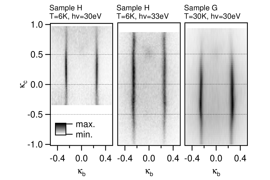
Figure 28: Three Fermi-surfaces out of the data which we use in the following analysis. The two first (similar to FIG. II 19) are from a sample H at T=6K measured at two photon energies $h\nu$=30 eV and 33eV, corresponding to $\kappa_{a}$=6.3 and 6.6, respectively. The last is from a sample G with $h\nu$=30 eV, $\kappa_{a}$=6.3. The figures have been stretched along $\kappa_{c}$ by a factor 1.7; compare with FIG.s II 11 and 20 (b), which are to scale.

In this section we describe our analysis of the ARPES data taken from the intensity cube $I(E,\kappa_{b},\kappa_{c})$. Fig. 28 shows the FS obtained from sample H at T=6K measured at the two photon energies $h\nu$=30 eV and 33eV, which correspond to $\kappa_{a}$=6.3 and 6.6, respectively, and from sample G with $h\nu$=30 eV, $\kappa_{a}$=6.3. We know from theory that the FS consists of the four values (left and right, inner and outer sheets) of the Fermi-momentum $\kappa_{Fb}$ as a function of $\kappa_{c}$ when the dispersion with $\kappa_{a}$ is neglected.

At first glance the experimental FS does not appear to have two sheets. However, one can clearly see by eye in Fig. 28 that the black vertical lines (representing the FS) are not exactly straight, but are slightly “breathing” inwards and outwards in a regular pattern. In the following, we will examine this breathing more meticulously. We will find that it is the result of our selection rule causing the observed FS to switch from one sheet to the other. Further, the shape of each sheet is found to be consistent with our theory. Nonetheless, as we have shown in past work [88, 18, 3], and as discussed further below, we emphasize that the FS is defined by dispersing lineshapes with non-Fermi liquid features that are generic to the TL model. The selection rule explains a puzzle from this past work, that we were able to analyze the lineshapes with a one-band TL spectral theory, even though there are actually two bands. We now understand that for most of k-space, ARPES sees only one band at a time. Before presenting and discussing the data in relation to our theory, we discuss the challenges and issues we are facing and explain the method we are using. This method also enables the $\kappa_{b}$-projected Fermi-velocity to be extracted as a function of $\kappa_{c}$.

XV.1 Challenges, issues, and methods used for the Fermi-surface determination

XV.1.1 LiPB-specific issues

As explained in detail in Sect. II IX, the ARPES intensities from the six $t_{2g}$ $\left(m=yz,xz,xy\right)$ bands in LiPB display fine- and coarse-grained variations.

While the two subbands of a given $m$ are periodic in the single zone, the fine-grained intensity modulation considered in Sect. II IX.2.1 follows the $\left|\mathbf{k}\right\rangle$-character, apart from the nearly canceling phase shifts from the inversion and displacement dimerizations. It is therefore almost periodic in the double zone (Fig.s II 11, 12, and 13), as if the ribbons had been translationally equivalent (Sect. I III.1) with the intensity from the lower $m$-band in the 1st zone and the intensity from the upper $m$-band in the 2nd zone. Due to the dimerization of the ribbons, the $m$-band is gapped at the physical zone boundary and the shift from one subband to the other of the dominating $\left|\mathbf{k}\right\rangle$-character takes place over a region around this boundary. This was illustrated in the bottom part of Fig. II 14 for $k_{b}$=0.225 and we now repeat this in Fig. 29, but only for $k_{b}$=0.245 and the two $\widetilde{xy}$-bands, i.e. those with energies less than $\sim$100 meV below $E_{F}.$ The tilde and the dark-red color indicate that these $xy$-like bands are hybridized with the valence(V)- and conduction(C)- $xz$-and $yz$-bands which give rise to the peak-, bulge-, and near-contact features first mentioned in Sect. XIV.2.1. The 2nd zone extends from $k_{c}$=$-1$ to $-0.5$ and from $0.5$ to $1,$ with the 1st zone inserted between them, from $-0.5$ to $0.5$. Only near the zone-boundaries, $k_{c}$=$\pm 0.5,$ does ARPES see both bands of which the lower has a large bulge whose minimum is split from the upper minimum by as much as 50 meV. The near contact between the two bands [sheets in Fig. 27 (d)] at $k_{c}$ integer is not directly seen in ARPES, because here, one of the bands (sheets) is extinguished, the upper band (inner sheet) at even $k_{c}$ and the lower band (outer sheet) at odd $k_{c}$. The resonance peaks in the upper band are clearly seen at $|k_{c}|$=0.76.

Since without the fine-grained ARPES intensity modulation, each band is periodic in the single zone (see Fig.s 25 and 26 top line to the right), symmetrization of the ARPES bands around the zone boundaries enabled us in Paper II to reconstruct the dispersions continuously (Fig.s II 20 and II 21). However, with $h\nu$=30 eV, the coarse-grained intensity of the $\widetilde{xy}$-bands falls off rapidly for $\kappa_{c}>0.5$, and this made it difficult, but –thanks to the fine-grained modulations– not impossible to detect the resonance peaks in the upper band [see Fig. II 24$($c2)]. Later, we realized that the spread of the Wannier orbital onto several molybdenums makes the coarse-grained intensity sensitive to the photon energy, which can therefore be choosen to yield good visibility over a sufficiently wide range of $\kappa_{c}$ and to produce cancellation between the inversion- and displacement phase shifts.

The ARPES intensity from the inner and outer sheets of the FS behaves like the intensity for respectively the upper and lower $\widetilde{xy}$-bands, as we shall see in Fig. 32. For extracting the FS, our present method to be described below, however fails near the zone boundaries because we have no good symmetrization scheme unlike for the bands. We can merely estimate the splitting at the boundary from the so-called Sparrow criterion used in astronomy [89]

To set the scale, we first recall from the theoretical FS in Fig. 27 (d) that even at $k_{c}$=0.5, the $k_{b}$-splitting between the inner and outer sheets amounts to merely 0.01$b^{\ast},$ i.e. to 2% of the distance between the left and right-hand FS sheets. The experimental Fig. 28 shows both left- and right-hand sheets and, here, the inner and outer sheets cannot be distinguished because the momentum-distribution widths of the two spectral functions of the bands are larger than their splitting (see Sect. II X.3.2). However, already in the data, we see a slight wrinkle around $\kappa_{c}$=$\pm 0.5$ caused by the shift of intensity from one band to the other.

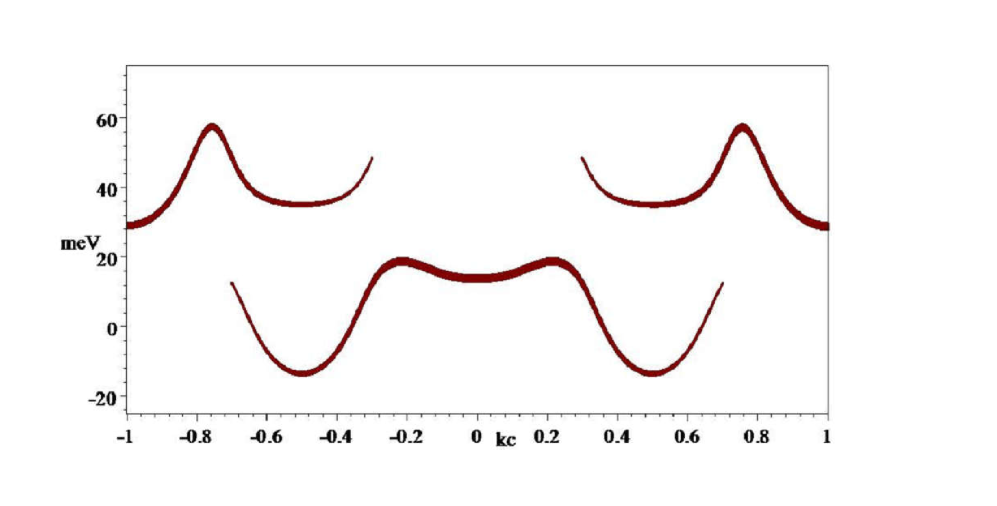
Figure 29: The $\widetilde{xy}$ bands in the double zone for the two-band Hamiltonian (121) with ARPES-refined TB parameters, like in the bottom panel of Fig. II 14, but only for the dark-red $\widetilde{xy}$ bands, for $k_{b}$=0.245, and on an extended energy scale with the upper frame at the Fermi level (75 meV). The fatness is proportional to the fine-grained band-factor ARPES intensity because for our particular case of $\kappa_{a}$=6.6, the dimerization phase shift, $\eta$ II (78), is negligible in the $k_{c}$-region of interest (see Fig. II 12).

There is a second issue specific to LiPB; it is a quasi-1D material and, at high enough temperatures, manifests a TL-like spectral function with a broad spinon edge feature and a somewhat sharper holon peak feature [18, 82, 3]. For the data here, the momentum integrated EDCs around $k_{Fb}$ gave a power-law like line-shape. Although the LiPB ARPES lineshape is well described by the TL spectral function at high temperature, the spectra do not sharpen as much as expected in the theory[82] at low temperature . Therefore our specific procedure, described below, follows a route in which no theoretical spectral function is forced onto the experimental data.

XV.1.2 General issues

Note that the change of momentum in $\kappa_{b}$, visible in Fig. 28, is small - we will see that it is in the range of 0.01 which translates to the experimentally very demanding range of 0.012Å^-1 using the solid-state definition (ssd) of reciprocal space (see Sect. III of Paper I). For our measurements, that is about the size of two detector pixels. We will see that it is very well possible to extract such a relative change from the ARPES data by our method. The determination of the absolute value of the Fermi-momentum and the filling is limited to a systematic error of about 1 % .

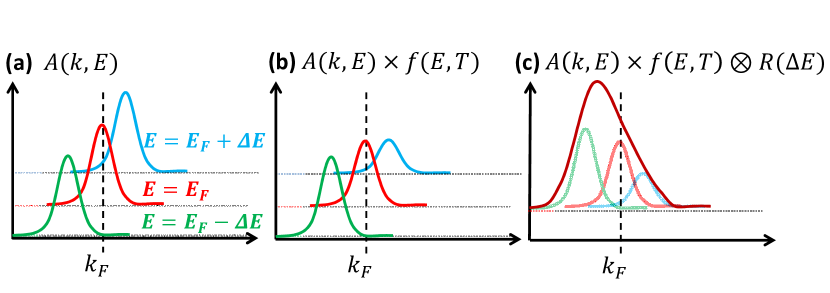
Figure 30: Sketch to explain a masking effect hindering the Fermi-momentum determination when only considering the maximum of the MDC at $E_{F}$. (a) Shown are three MDC’s for different energies as indicated around $E_{F}$. In (a), the spectral function give perfectly symmetric and Lorentzian-like MDC’s. The combined effect of (b) the distribution function $f(E)$, and (c) convolution with the energy resolution $R(\Delta E$) results in a an asymmetric line-shape for the MDC at $E_{F}$ (dark red in (c)).

In order to obtain the value of the Fermi-momentum, one may think that it suffices to determine the peak maximum of the MDC at $E_{F}$. In reality, the exact determination of the Fermi-momentum is an important issue warranting discussions to be found in e.g. Refs. 90, 91, 92, 93, 94. There are many intrinsic and extrinsic reasons not to determine the correct $k_{Fb}$. Particularly important for us is a masking effect in extracting the Fermi momentum which occurs rather generally and does not depend much on whether the sample is a Fermi-liquid, marginal Fermi-liquid, or a TL-liquid. This effect is sketched in Fig. 30: Even if (a) the ARPES spectral function is perfectly symmetric and Lorentzian-like in the momentum direction, the combined effects of the distribution function (e.g. the Fermi function) (b) and the convolution with the experimental energy resolution (c), results in an asymmetric line-shape for MDC’s for energies near $E_{F}\pm\Delta E$. Here, $\Delta E$ represents the experimental energy resolution, which for $h\nu$=30 eV is 16 meV (Sect. X.3.2). Hence, the asymmetry causes the peak momentum to be inside the FS.

XV.1.3 Method

With these considerations in mind, we now explain our methods. It is important to mention again that theory dictates that we cannot distinguish the two bands but obtain an average dispersion weighted by the ARPES band-factor intensity, the $\left|\mathbf{k}\right\rangle$-character shown in Fig. 29. This means that for $|\kappa_{c}|<0.35$, we are mainly extracting the outer FS sheet (lower band) while for $0.65<\left|\kappa_{c}\right|$, we mainly extract the inner sheet (upper band). Thus, like for the bands, the selection rule allows us to distinguish the two FS sheets, except near the zone-boundary, $\left|\kappa_{c}\right|$=0.5, where the intensity shifts from one band to the other. We first discuss, in Sect. XV.1.3, what can be deduced for the zone-boundary situation, using the Sparrow criterion [89] to analyze the MDC widths. This exercise will bring out the fact that the experimental MDC widths greatly exceed the splitting that we wish to determine and thereby make clear the crucial role of the selection rule, which we exploit in Sect. XV.1.3, using a so-called dispersion analysis, to determine the Fermi momentum as well as the Fermi velocity of separate branches.

Sparrow MDC peak-width analysis:

At the zone boundaries, $\left|\kappa_{c}\right|$=0.5, although we have no way to separate the inner and outer FS sheets, we can nonetheless estimate their possible splitting, as we now describe. As follows from the fine-grained intensity modulation of the two $\widetilde{xy}$-bands discussed in Sect. II IX.2.1 and displayed in Fig. 29, the MDC at $E_{F}$ for $\kappa_{c}$=0.5 (or $-$0.5) is an equally weighted combination of the Lorentzian-like MDC’s of both sheets and, as the combination, has the measured total width $\Gamma_{MDC}^{\kappa_{c}=0.5}.$ With this, we can use the so-called Sparrow criterion [89], which states that two identical, separated Lorentzians of the same width $\Gamma_{MDC}^{j=1}=\Gamma_{MDC}^{j=2}$ are indistinguishable if they add up to give a flat top with zero slope and curvature at their center of mass. These conditions allow computing a splitting ($\Delta\kappa_{b}$) as well as the width of the two Lorentzians ($\Gamma_{MDC}^{1/2}$) from the measured total width ($\Gamma_{MDC}^{\kappa_{c}=0.5}$). In fact, it will be an upper limit for the splitting and reads: $\Delta\kappa_{b}^{\kappa_{c}=0.5}=\Gamma_{MDC}^{\kappa_{c}=0.5}/\sqrt{3}$. The two Lorentzian have a width of: $\Gamma_{MDC}^{j}=\Gamma_{MDC}^{\kappa_{c}=0.5}\,\sqrt{3}/(1+\sqrt{3})$. The results of this Sparrow analysis are given in Tab. 1 and also indicated by the diamonds in Fig. 32. From the table, by seeing that the measured MDC-widths at zone-boundary ($\Gamma_{MDC}^{\kappa_{c}=\pm 0.5}$) and zone-center ($\Gamma_{MDC}^{\kappa_{c}=0}$) are almost the same, we can already see that there is a limit to the determination of the splitting. The MDC’s are obviously broad. This broadening is much more than the momentum resolution of the apparatus ($\Delta\kappa_{b}\approx$ 0.005, see Sect. II X.1). The broadening can be for different reasons. There is an intrinsic component by the spectral function of the corresponding electron liquid. In the case of a Luttinger-liquid, it is well known (see, e.g., Ref. 95) that the MDC’s are typically sharper, and the EDC’s are broader (when compared to a Fermi-liquid). However, there can also be an extrinsic component –by an experimental momentum resolution which is not produced by the apparatus alone but, for example, can be caused by the quality of the samples-surface and the so-called $k_{z}$-broadening [96, 97] that arises from the limited probing depth of the photoelectron. In general, it is hard and requires multiple experiments to distinguish the intrinsic and extrinsic components with full certainty. Looking at the widths for different samples, displayed in Tab. 1, we can believe that there is a larger intrinsic component but also some extrinsic component.

We reiterate that the resulting separation estimate by the Sparrow criterion is an upper limit and the actual splitting has to be below the smallest splitting listed in Tab. 1, resulting in $\Delta\kappa_{b}^{\kappa_{c}=0.5}<0.017$. By taking advantage of the selection rule, we will see that this is indeed the case, and we note now that even this upper limit is considerably less than the magnitude of the experimental MDC width at $\kappa_{c}=0$, where the selection rule applies and only one branch contributes.

Sample		$\Gamma_{MDC}^{|\kappa_{c}|=0.5}$	$\Gamma_{MDC}^{j}$	$\Gamma_{MDC}^{\kappa_{c}=0}$	$\Delta\kappa_{b}^{|\kappa_{c}|=0.5}$
H 6K,30 eV	+	0.030	0.0191	0.031	0.017
H 6K,33 eV	+	0.047	0.030	0.051	0.028
	-	0.044	0.028	0.051	0.025
G 30K,30 eV	+	0.060	0.038	0.052	0.035
	-	0.051	0.033	0.052	0.030

Table 1: Result of the MDC peak-width analysis (compare also with Fig. 28). The 1st column gives the individual dataset, the 2nd indicates whether $\kappa_{c}$=$+$0.5 or $\kappa_{c}$=$-$0.5 was measured. Column 3 gives the Lorentzian-width $\Gamma$ obtained by a line-fit and is averaged over both branches, at positive and negative $\kappa_{b}.$ Column 4 gives the width of the two Lorentzian ($\Gamma_{MDC}^{j}$) at $\kappa_{c}$=$\pm$0.5 according to the Sparrow criterion. The 5th is the Lorentzian-width at $\kappa_{c}$=0. The last column, finally, shows the upper limit for the separation in $\kappa_{b}$ momentum ($\Delta\kappa_{b}^{\kappa_{c}=0.5}$) according to the Sparrow-criterion.

Dispersion Analysis:

Figure 31: Method used for the extraction of the Fermi-momentum. The experimental data set is sliced along the $\kappa_{c}$-direction (bottom). Each $\kappa_{c}$-slice can then be viewed as containing multiple so-called MDC’s. The MDC’s are intensity curves at fixed energy, dependent only on $\kappa_{b}$ (see the magenta curves in the upper right as examples). Then, a line fit with a Lorentzian for all the MDC’s between $E_{F}-50~{}$meV and $E_{F}$ was performed. The maximum of the Lorentzian defines the dispersion $E(\kappa_{b},\kappa_{c}=const.)$ (upper left). The Fermi-momentum $\kappa_{Fb}$ is found by linear extrapolation in this interval between $E_{F}-50~{}$meV and $E_{F}$ (see red extrapolation line and red circle at $k_{Fb}$ in upper left).

	used		Li-
Sample	$\kappa_{c}$-range	$k_{Fb}^{avg}$	stoichiometry
H 6K,30 eV	0 ; 0.995	$0.255\pm 0.006$	$1.02\pm 0.02$
H 6K,33 eV	-0.785; 0.905	$0.254\pm 0.005$	$1.02\pm 0.02$
G 30K,30 eV	-0.824; 0.777	$0.255\pm 0.008$	$1.02\pm 0.02$
Average		$0.255\pm 0.006$	$1.02\pm 0.02$

Table 2: Extracted absolute average Fermi-momentum $k_{Fb}^{avg}$ (3rd column) and the Li-stoichiometry from the electron filling (last column). The 1st column identifies the dataset used, the 2nd column the span of $\kappa_{c}$ over which the average was taken (cf. FIG. 32). The error given here is the error of determining the average and does not include the variation of $k_{Fb}(\kappa_{c})$ with $\kappa_{c}$. The last column gives the Li-stoichiometry from the Luttinger count of the FS, including its error in determination.

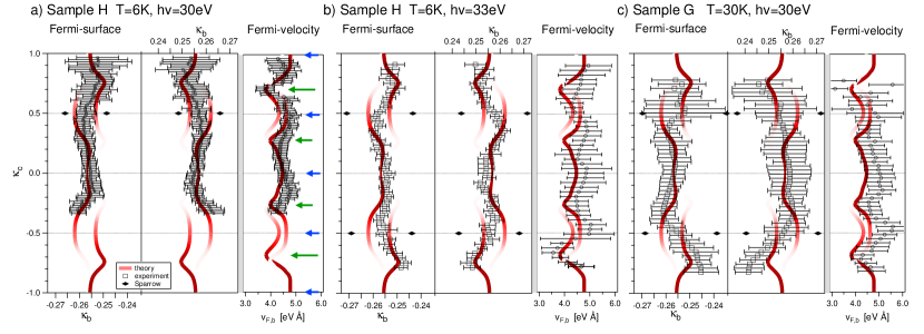
Figure 32: Results of the Fermi-momentum extraction (black points with error bars, see Sect. XV.1.3) in the double zone and for each individual dataset, as indicated. For each set, the larger panel shows the four FS sheets (left and right, outer and inner), while the smaller panel shows the $k_{b}$-projected velocity (128) averaged using the left and right $k_{b}$-projected velocity. Underlayed in dark red with an intensity proportional to the $\left|\mathbf{k}\right\rangle$-character [Eq. II (79) with $\eta$=0, i.e. Eq. I (63)] are the theoretical FS [Fig. 27 (d)] and its $k_{b}$-projected Fermi-velocity. Also included in the graphs for the FS are the results (Tab. 1) of the Sparrow analysis for the maximum splitting at the zone boundary. $\kappa_{a}$=6.3, 6.6, 6.3 in respectively a), b) and c). Each theoretical and experimental FS has been compressed by a factor 11 along $\kappa_{c}.$

The method used to extract the Fermi-momentum $\kappa_{Fb}$ as a function of $\kappa_{c}$ is basically to extrapolate the metallic ARPES band along $\kappa_{b}$ for fixed $\kappa_{c}$ to the Fermi level (Fig. II 21). The details are sketched in Fig. 31. The experimental data set is sliced along the $\kappa_{c}$-direction; see the slices on the lower part of the figure. Each slice can be seen as a set of so-called momentum distribution curves (MDC’s). An MDC (see also Sect.XI in Paper II) is the photoelectron-intensity at fixed energy, here only dependent on $\kappa_{b}$ (see the magenta curves in the upper right of Fig. 31 as examples for MDC’s). For the analysis, we choose now to use all MDC’s with energies between $E_{F}-$50 meV and $E_{F}$ (the separation $\Delta E$ was typically 5 meV). We then fit each MDC (on each dispersion branch) with a Lorentzian. The maximum position of the Lorentzians defines the dispersion (indicated by the purple lines in the upper left of Fig. 31). We interpolated the Fermi-momentum ($\kappa_{Fb}$) by a line-fit with the linear function $\kappa_{b}=(E-E_{F})/v_{F}+\kappa_{Fb}$ (see red line in upper left of Fig. 31). By this line-fit we remove the error arising from the masking-effect discussed above (see Fig. 30) which appears as a ”kink” near the value of the energy resolution. In accordance with the energy resolution of about 16 meV, the kink sets in at (see blue arrow) $E-E_{F}\approx 13~{}$meV in Fig. 31.

The dispersion analysis offers a notable advantage in terms of statistical certainty, primarily due to the utilization of a broader data range spanning 50 meV. For the analysis of TL-liquid performed here, this holds particular significance as the density of states exhibits a power-law decay as it approaches E_F. Furthermore, the dispersion analysis also gives naturally an estimate of the $\kappa_{c}$-dependence of the Fermi velocities projected onto the $\kappa_{b}$-direction,

$$\mathbf{v}_{F\,j}\left(k_{c}\right)\cdot\mathbf{b}^{\ast}/b^{\ast}\equiv\partial E_{j}\left(k_{b},k_{c}\right)\left/\left(\partial k_{b}b^{\ast}\right)\right|_{E_{F}}.$$ (128)

The result of this extraction method is displayed in Fig. 32 and Tab. 2.

XV.2 Results of the Fermi-surface determination and Comparison with Theory

XV.2.1 Fermi-surface

The result of the Fermi-momentum extraction is displayed in Fig. 32. It compares the experimental FS (black points with error bars) with the theoretical FS (dark-red) calculated using the two-band Hamiltonian (121) with the ARPES-refined parameter values and drawn with the fine-grained intensity proportional to the $\left|\mathbf{k}\right\rangle$-character I (63) because for $\kappa_{a}$=6.3 and 6.6 the dimerization phase shift $\eta\left(\mathbf{\kappa}\right)$ is neglible (see Sect. II IX.2.1 Eq. (79) and Fig. 12).

We see that the Fermi-momentum extracted from ARPES fits beautifully with the theoretical FS sheet of dominating intensity: In all three measurements, it aligns with the outer sheet for $|\kappa_{c}|<0.35$ and with the inner sheet for $|\kappa_{c}|>0.65.$ Near the zone-boundaries, $\left|\kappa_{c}\right|$=0.5, where the dominating intensity shifts from one sheet to the other, so does the experimentally extracted $\kappa_{Fb}$. Also, the general shape of the experimental FS fits nicely with the prediction by theory. This is, on the one hand, not astonishing as we use ARPES-refined parameter values, but on the other hand, the refinement was done for features well away from the Fermi energy, and yet, all details of the theoretical FS (seen in Fig. 27 (d) and described in Sect. XIV.3) are seen in the experiment, with the exception of the near contact between the inner and outer sheets, which does require interpolation of the former to $k_{c}$=0 or extrapolation of the latter to $k_{c}$=1. Later on, we will discuss this also for the Fermi-velocities.

The experimental upper bound given by the Sparrow criterion on the splitting between the inner and outer sheets at the ZB, $\left|\kappa_{c}\right|$=0.5, is indicated by the black diamonds. It is consistent with, but considerably larger than, the theoretical splitting.

As can be seen from Tab. 2, for all three samples, $k_{Fb}$ averaged over $k_{c}$ gives a Luttinger volume which corresponds to an effective Li_1.02±0.02 stoichiometry, i.e. an electron filling of $0.51\pm 0.01$. This places the Fermi level 75 meV above the center of the gap in the calculation.

We note that the procedure of refining the values of the TB parameters to fit the ARPES dispersions for energies more than 0.15 eV below $E_{F}$ in one sample does well in describing the dispersions for energies closer to $E_{F}$ than 0.15 eV in all three samples. This is a testimonial, both to the reproducibility of our findings for samples from different sources and to the essential role that resonant coupling to the higher-energy gapped $xz$ and $yz$ bands plays in determining the dispersion and splitting of the metallic $\widetilde{xy}$ bands.

Finally, we take notice of a very recent publication [99] reporting transport data interpreted as showing a FS reconstruction resulting in a semi-metal FS below 100K. The modeling for this very interesting proposal was based on our analysis, reported in Ref. 100 (Sect. VI E) , of possible nesting and gapping of the metallic FS, which however concluded that complete SDW gapping requires an effective exchange interaction about three times the value given by the local spin-density approximation (LSDA) and is therefore unlikely.

We point out, as is also acknowledged in Ref. 99, that the 6K ARPES data reported here and in Ref. 100 do not show any evidence for such a FS reconstruction and that our measured Fermi velocity ($\sim$4.6 eVÅ$\approx$7$\times$10⁵ m/s) which was shown as the slope of the unreconstructed, weak bands in Fig. 15 of Ref. 100 and of the dashed bands in Fig. S10 (c) of Ref. 99, is several times larger than those ($\sim$2$\times$10⁵ m/s $\approx$1.3 eVÅ) for the gapped bands at the Fermi level in Fig.s 15 and S10 (c).

XV.2.2 Fermi-velocity

To the right of each FS in Fig. 32, we show the $k_{c}$-dependence of the $k_{b}$-projected Fermi-velocity, defined by Eq.(128: in black, as extracted from ARPES and in red, as calculated with the two-band Hamiltonian.

Overall, we see a good qualitative correspondence between the theoretical and the experimentally extracted values. For those $k_{c}$ values where the $k_{b}$ direction is normal to the FS, the velocity projection (128) has extrema. At the zone centers ($k_{c}$=integer) and zone boundaries ($\left|k_{c}\right|$=0.5) –indicated by blue arrows in Fig. 32– these extrema are flat maxima. For the inner-sheet (upper-band) notches (green long arrows at $\left|k_{c}\right|\approx$0.75), the extrema are deep minima. Also the outer sheet (lower band) has velocity minima (green short arrows at $\left|k_{c}\right|\approx$0.30). Their origins are the weak resonance peaks at $\left|k_{c}\right|\approx$0.25 (see Fig. 29 and Eq. (127)), combined with the increase of $\left|\mathbf{k}\right\rangle$ - $\left|\mathbf{k+c}^{\ast}\right\rangle$ hybridization and the concomitant formation of bulges as the zone boundaries at $\left|k_{c}\right|$=0.5 are approached.

The velocity of the outer sheet (lower band) decreases from 4.5 eV Å at the zone center ($k_{c}$=0) to the 4.0 eV Å deep minima near $\left|k_{c}\right|$=0.30, and rises again to the 4.6 eV Å maxima at the centers of the bulges, $\left|k_{c}\right|$=0.5. For the inner sheet (outer band), the velocity decreases from 4.7 eV Å at the zone centers ($\left|k_{c}\right|$=1), to 3.9  eV Å deep minima near the notches, and rises again to 4.3 eV Å maxima at the zone boundaries. These sheet- and $k_{c}$-dependent values may be compared with the dominating value 4.6 eV Å of $b\tau^{\prime}\left(k_{b}\right)$ in Eq.s I (50) and (VI.1) from the direct hopping along the ribbon. Due to the indirect hops via the valence and conduction bands giving rise to the resonance terms in Eq. (121), the band- and $k_{c}$ average of the velocity projections is smaller than $b\tau^{\prime}\left(k_{b}\right)$. The velocities extracted from the ARPES data (black) clearly show both the qualitative behavior and the general magnitude implied by the theory (dark-red). To a small extent, this is expected since, as explained in Sect. I XI and specified in Tables I 43 and 45, a few of the many LDA TB parameters were refined to make the bands agree with the large- but not the small-energy features of the ARPES bands.

It is also interesting for the many-body physics of LiPB to compare the experimental velocities to those for the TB bands based on the LDA parameters. The LDA dominant velocity value is 4.0 eV Å. The experimental velocities (and those for the ARPES-refined TB) are generally greater than those for the LDA by about 15%.

There are two points to be made. First, for a 3D quasi-particle material the increase of the experimental velocity relative to the LDA value would seem surprising since the usual effect [86], arising from an energy-dependent single-particle self-energy, e.g., caused by ${e}$-${e}$ or ${e}$-${ph}$ interactions, is an increase of the Fermi-mass, i.e. a decrease of the Fermi velocity . Indeed such was found in the single-site DMFT quasi-particle treatment of LiPB [19]. However, LiPB is a quasi-1D material whose ARPES $k$-averaged lineshapes show TL-model properties, i.e. quasi-particle suppression and spin-charge separation. Specifically, the holon-peak and spinon-edge features disperse with different velocities, $v_{\rho}$ and $v_{\sigma}$, respectively [14, 95, 103]. Our model-independent ARPES analysis procedure, if performed on a TL-lineshape, would yield a dispersion intermediate between $v_{\rho}$ and $v_{\sigma}$, but tending mostly to that of the holon peak. Within 1D theory, $v_{\rho}$ and $v_{\sigma}$ can just as well be either larger or smaller than the underlying $v_{F}$ of a non-interacting system, as can be seen, for example from formulas within the framework of the “g-ology” formulation [104, 95]. So if we identify the LDA value of $v_{F}$=4.0 eV Å as “non-interacting,” which ignores the difficulty of disentangling any many-body contribution already present in LDA, and think of our ARPES lineshape in a TL context, it is well within general theoretical expectations that our experimental velocity is larger than the LDA value. In this view, it may well be that our ARPES-refined TB description is modifying the entire $k_{b}$ dispersion somewhat in order to reproduce the experimental low-energy scale velocity near $E_{F}.$

Second, combining our results with a previous ARPES lineshape analysis [88], we can be somewhat more precise about the velocity renormalizations for LiPB. At high temperatures, where the LiPB ARPES lineshapes are well described by TL lineshape theory [103] for nonzero $T$, the best TL description [88] for the $\Gamma$-Y ($k_{c}$=0) ARPES lineshapes was achieved for $v_{\rho}/v_{\sigma}$=2. At that time no definitive LDA value of $v_{F}$ was available. If we now think of our ARPES velocity as being nearly that of $v_{\rho}$, and take our LDA velocity as an underlying “non-interacting” $v_{F}$, then –at least for $\Gamma$Y– we conclude that $v_{\rho}$ is roughly 1.15$v_{F}$, and that $v_{\sigma}$ is roughly 0.6$v_{F}$ . A 1D Hubbard-model analysis [17] estimated $v_{\sigma}/v_{F}\approx J/2\tau$ with $J\approx 0.2~{}$eV being an effective super-exchange interaction, and $\tau\approx 0.8~{}$eV being the primary $k_{b}$ hopping, implying $v_{\sigma}/$ $v_{F}\approx 1/8.$

XV.2.3 Connecting to the TL critical exponent $\alpha$

As already written in the introduction of Paper I, LiPB displays Luttinger liquid properties. Most remarkably, although the FS is well defined and could be extracted above, the lineshapes are better described by a TL spectral function. Nevertheless, there are also substantial $T$-dependent departures from the TL model. The ARPES line shapes at temperatures 250K to 300K are well described by the TL spectral function, showing both spinon and holon features (broadened by temperature and experimental resolution). With decreasing $T$ the exponent varies with $T$, from $\alpha=0.9$ at 250K to $0.6$ at 50K, and also, the ARPES lineshape no longer agrees with the TL lineshape, although it does continue to display quantum critical scaling, a characteristic 1D property [18]. The spectra for $k$-integration along the quasi-1D direction, for temperatures $T$=4K and 30 K and resolution 5 meV, are well described by a power law with $\alpha=0.7$ [3].

In the following, we repeat the analysis of Ref. 3 with our recent data sets used to determine the FS above. However, in the course of the present study, we found that (i) all previous TB ladder models are very unrealistic, and (ii) the detectable bands of ARPES vary with fine-grained intensity proportional to the $\left|\mathbf{k}\right\rangle$-character. In principle, these findings should inform the choice of a particular TL model. For the phenomenological extraction of the $\alpha$ value, however, we still use the same procedure as in Ref. 3 to obtain its value. As before, we use the $\kappa$-integrated spectral weight of a one-band, spin-rotational invariant TL-model [103] with $v_{\rho}/v_{\sigma}$=2. The theoretical spectrum was broadened by the experimental energy resolution of 16 meV.

The data displayed in Fig. 33 are integrated over $\kappa_{b}$ and $\kappa_{c}$ (cf. Fig.28). For the $\kappa_{c}$-direction, the data are integrated over two intervals, according to whether the dominant character is $\left|\mathbf{k}\right\rangle$ or $\left|\mathbf{k+c}^{\ast}\right\rangle$. As visible in Fig. 33, sample G (T=30K) shows a typical value of $\alpha=0.70$ for both intervals. The data for sample H (T=6K) vary a bit more on the two intervals but are still within the error range, yielding in average $\alpha=0.58$. Connecting to the study of Ref. [18], despite a considerable difference in the determined $\alpha$-values for samples G and H, these values are within the $\alpha$-ranges of former studies. To shed light on more details, temperature-dependent measurements in the full range of relevant momenta would be required as well as the usage of a more realistic TL model than the one-band, spin-rotational invariant TL-model for the line-fit.

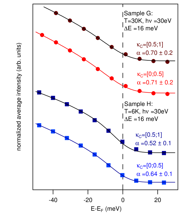
Figure 33: Analysis of the TL-exponent of the data for sample G (T=30K) and H (T=6K). The FS’s were presented in Fig. 28. Here the data is momentum-integrated over two intervals, where the dominating band character is either $\left|\mathbf{k}\right\rangle$ or $\left|\mathbf{k+c}\right\rangle^{\ast}.$

XVI Interactions and correlations

As described in the first paragraph of Paper I, for interacting electrons that can only propagate in one spatial dimension Landaus Fermi-liquid (FL) theory does not hold [13, 12, 14]. Instead one finds a correlated Luttinger-liquid (LL) system with a zero density of states at the Fermi energy. Furthermore, the density of states increases at finite energy away from the Fermi energy following a Tomonaga-Luttinger (TL) model line-shape characterized by an anomalous exponent $\alpha$. As shown in Fig. 1 of paper I and Fig. 33 of paper III we indeed observe such a line-shape of the density of states below the Fermi energy in LiMo₆O₁₇. Although this LL behavior occurs for even an infinitesimally small Coulomb interaction, nonetheless the actual magnitude -and also the range- of the interaction is important because these determine the values of correlation function power laws such as $\alpha$, as well as other possible properties of the actual interacting state in any particular material. Thus it is generally important to try to make an estimate of the interaction strength and range.

Using constrained DFT Popovic and Satpathy[25] showed that the Coulomb interaction $U$ between two electrons in atomic d-like orbitals of Mo in LiPB is $U_{Mo-d}$ = 6.4 eV. Constrained RPA calculations for a dense f.c.c. lattice of atomic Mo yield a value of $U_{Mo-t_{2g}}$ = 3.7 eV for the atomic-like $t_{2g}$-orbitals of a single Mo atom [105]. However, it is important to realize that the Wannier orbitals that build the one-dimensional bands are far from being atomic and localized on a single Mo atom. As we showed the smallest tight binding model one can make for LiMo₆O₁₇ considers 6 bands per unit cell, and the resulting Wannier orbitals spread over several unit cells (see Figs. 5 and 9 of paper I). Thus, the parameter determining the Coulomb interaction strength for the Wannier orbitals will be smaller than the Coulomb parameter for a single atomic Mo orbital, due both to the dilution of the charge density to several Mo atoms and to screening. Calculating the screened Coulomb interaction between such large Wannier orbitals for a material with many atoms per unit cell is a daunting task. Neither accurate constrained random phase approximation nor constrained density functional theory calculations seem feasible with the currently available codes.

Whilst it is computationally difficult to reliably calculate the screened Coulomb interaction of such large Wannier orbitals, one can very well calculate the bare Coulomb interaction. We have made this calculation and the result is $U^{Bare}_{Mo-W_{xy}}=2$ eV. We can easily rationalize this result by noting that the bare Coulomb interaction (F0) for the atomic 4d orbitals in Mo is $U^{Bare}_{Mo-d}=12.5$ eV and that the Wannier orbitals in LiPB are spread over several (5+) Mo atoms. Due to the large spread of the Wannier function the bare value of the nearest neighbor Coulomb interaction $V$ (and also those for even further distant neighbors) will be smaller, but still sizeable compared to $U.$ Noting that the bare value of $U^{Bare}_{Cu-d}=25$ eV for strongly correlated cuprates and is $U^{Bare}_{C-p}=14$ eV for graphene gives a useful perspective on the much smaller value of the bare $U$ in LiPB. We should warn the reader here that this value $U^{Bare}_{Mo-W_{xy}}=2$ eV is not the value one should use in a model calculation. The bare interaction sets a clear upper limit but should be greatly reduced in the material due to solid state screening. As a guide to the possible magnitude of the screening effect, we note again that Popovic and Satpathy calculated a screened value of 6.4 eV for atomic Mo in LiPB, roughly half the bare atomic value $U^{Bare}_{Mo-d}=12.5$ eV. A similar screening reduction down from the bare 2 eV value for our Wannier orbitals is expected.

The small value of the Coulomb interaction between the extended Wannier orbitals also explains why we experimentally find that the $xz$ ($yz$) and $XZ$ ($YZ$) bonding orbitals are doubly occupied forming an $S=0$ state instead of favoring a Hunds rule ground-state triplet state with $S=1$ where one electron is in the $xz$ ($XZ$) orbital and one electron in the $yz$ ($YZ$) orbital with parallel spin. One should not compare the gap $4G_{1}\sim$ 400 meV (Eq.s (29), (35), and (45) in Paper I) to the bare atomic interaction strength, but to the greatly reduced interaction strength of the Wannier functions due to the spread of the Wannier function over several Mo atoms within the unit cell.

For LiPB there are a number of previous theoretical studies aimed at understanding its various interesting strongly correlated quasi-1D properties [4, 17, 5, 6, 7, 9, 10, 20, 21]. Some of the various studies take specific values for $U$- and $V$-type interactions, for $U$ in a range from the Popovic-Satpathy value of 6.4 eV down to 1 eV, and for $V$-type interactions in the range 0.5 eV to 1 eV. It is not our purpose here to give any critique of these various models, which are elegant and creative, but the magnitude of the Coulomb interaction for our Wannier orbitals is supportive of the models which take $U$ at the low end of the range. The experimental $\alpha>1/2$ can be rationalized with both large and small values of $U$ [5, 6], but in so doing, a role for $V$-type neighbor interactions is essential, because for a simple single-chain Hubbard model the maximum value of $\alpha=1/8$ is obtained only for infinite $U$. The $V$-type values used are all generally consistent with our findings.

We note that Ref. [19], using the variational cluster approximation (VCA) and dynamical mean field theory (DMFT), found that for values of $U_{Mott}$ exceeding 0.7 eV and 2.5 eV, respectively, a Mott-Hubbard gap opens in their LDA bands, glaringly inconsistent with experiment, and therefore giving a clear upper limit. They note that the DMFT (VCA) overestimates (underestimates) $U_{Mott}$, so the two methods provide a range for an upper limit on $U$ for the 4-orbital set of Ref. [19]. Roughly, we expect that a set reduced in size by a factor of $n$ will be $n$-times less localized, with $U$ about $n$-times smaller, implying for our final 2-orbital set a general reduction in Coulomb energies by a factor of 2/4=1/2, relative to the 4-orbital set of Ref. [19]. Thus our conclusion on the smallness of $U$ is generally consistent with the findings of Ref. [19].

Ref. [19] also emphasized that the two metallic bands are half-filled. This question is important because most of the theories cited above assume no $b$-dimerization, i.e. assume that Mo(1) and Mo(4) are equivalent, and thereby view the two metallic bands as being quarter-filled. We agree with this emphasis in Ref. [19], in the sense that the dimerization gap is 0.7 eV, nearly 20% of the entire bandwidth (see Sect III B in Paper I). But there is some nuance. The motivation in the theoretical models is to make contact with a property of the quarter-filled Hubbard model, that of so-called 4k_F charge fluctuations, or even charge ordering, resulting from the $V$-type interactions. Dimerization is known to greatly diminish the tendency to such charge fluctuations [106], i.e. the two compete. The fact that the estimated magnitudes of the $V$-type interactions are in fact comparable to the dimerization gap implies that the relevance of the quarter-filling scenarios is not ruled out, presumably depending on details. So on the theory side, further assessment using more realistic modeling is essential. On the experimental side, Ref. [5] proposes measurements to directly search for the 4k_F-charge-fluctuations.

XVII Conclusion and Implications

In conclusion, we have presented in great detail the electronic structure of LiMo₆O₁₇ that is experimentally obtainable using ARPES, emphasizing the degree of one-dimensional behavior of the bands in the vicinity of $E_{F}$  and the excellent overall agreement with the LDA band structure. With the aim of fully describing and understanding the metallic bands found in the ARPES experiment, especially the details of FS splitting and warping, the LDA electronic structure was downfolded to a tight-binding description with the three Mo1-centered $t_{2g}$ Wannier orbitals (WOs) per formula unit (Sect. I VI) using the newly developed full-potential version of the NMTO method (Sect. I II). This description is based on analyzing the LiPB crystal structure as built from corner-sharing MoO₆ octahedra forming a staircase running along $\mathbf{c}$ of bi-ribbons extending along $\mathbf{b}$ (Sect.  I III).

The six $t_{2g}$ WOs per primitive cell accurately describe not only the four bands seen by ARPES, but all six bands in the 1 eV neighborhood of $E_{F}$. This band structure (Sect. I IV and Fig. I 4) is basically 2D and formed by the $xy,$ $xz,$ and $yz$ WOs (Fig. I 9) giving rise to three 1D bands running along respectively $\mathbf{b},$ $\mathbf{c}\mathbf{+b},$ and $\mathbf{c}\mathbf{-b},$ i.e. at a 120^∘ angle to the two other bands (Fig.s I 8 and II 20). The dimerization from $c/2$ to $c$ of the ribbons into bi-ribbons gaps the $xz$ and $yz$ bands and leaves the $xy$ band metallic in the gap, but resonantly coupled to its edges and, hence, to the $\mathbf{c}\mathbf{+b}$ and $\mathbf{c}\mathbf{-b}$ directions. Inclusion of the $xz$ and $yz$ bands are indispensable in describing the strong indirect contributions to the $k_{c}$-dispersion and splitting of the metallic $xy$ bands. These are most prominent (see Fig.s I 8,  II 20, and  III 32) at the crossing of the $xy$-band CECs running parallel to the $\mathrm{P}_{1}\mathrm{Q}_{1}\mathrm{P}_{1}^{\prime}$-line ($k_{b}$=0.225$)$ in reciprocal space with those of the $xz$ and $yz$ V&C-band edges along respectively $\mathrm{ZY}^{\prime}$ and $\mathrm{ZY.}$ All the ARPES-measured dispersions, as well as the FS, indeed confirm the resonant indirect couplings and thus the essential need for the six-band picture. The TB bands are very well described by an analytic 6$\times$6 Hamiltonian I (35) or (56) with parameters optimized to match the ARPES data for energies more than 0.15 eV below $E_{F}$. Finally, the mix of direct and resonant indirect couplings along the $\mathbf{c}$-direction can be explicitly displayed by further analytical downfolding to the effective 2$\times$2 Hamiltonian III (121). This and direct observation by ARPES is compelling evidence for the existence of pronounced resonance structures near $E_{F}$ in LiPB.

In section XVI, we have presented some implications of our results specifically regarding interactions and correlations. In addition, there are four important implications for the general questions posed in the Introduction of Paper I. These implications follow directly from the central content of the paper, our new knowledge, and understanding of the size of the splitting and perpendicular dispersions of the quasi-1D bands in the gap (Fig.s III 25 and 26), especially the indirect resonance contributions. They have been stated already in the flow of the presentation, and we merely summarize them here.

First, the reality of the resonance contributions casts serious doubts on theoretical descriptions based on TB bands which are featureless like the red ones in Fig.s 25 and 26, i.e. casts doubt on all previous TB and TL models. Further, in constructing an appropriate many-body Hamiltonian, it should be taken into serious consideration that with ARPES, we have now been able to follow the resonance peak induced by the valence band to energies nearly 150 meV below the Fermi level (Fig. II 20) and, there, find the peak to have a magnitude of about $50$ meV, as predicted by the LDA, cf. Fig. II 24 (c2).

Second, the general magnitude of the $t_{\perp}$ -hoppings would suggest that 1D to 3D crossover should occur for $T$ as high as at least 150 K, unless thwarted by the theoretically expected strong downward low-$T$ renormalization due to LL fluctuations on the chains, as pointed out in the Introduction. However, the good agreement between LDA and ARPES data at $T$=6 K implies that this renormalization does not take place. This circumstance is not only puzzling, given the evidence for LL effects on the chains at high $T$, but eliminates one very attractive explanation for the exceptional stability of quasi-1D behavior in this material. Our new quantitative knowledge of the $t_{\perp}$-hoppings further emphasizes this puzzle.

Third, the coupling of the quasi-1D bands to the V&C bands causes the details of the FS splitting and warping (Fig.s 27 and 32) to depend strongly on the position of $E_{F}$ which in turn depends on the Li concentration. This implies that any property sensitive to the details of the FS will be very sensitive to the stoichiometry. One can then speculate that this FS sensitivity is connected to the sample dependence of the SC, especially if the SC is the product of the quasi-1D nature of the FS. We have already noted that the actual position of $E_{F}$ in LiPB is such as to maximize the quasi-1D nature of the FS. This could be an important addition to the various previous theories of the SC [20, 21, 6, 7, 9].

Fourth, the spatial dependence of the $t_{\perp}$-hoppings argues strongly against coupled ladder models of the chains. At the simplest level, the magnitude of the direct terms for hoppings within and between bi-ribbons (Sect. I IV) differ by less than a factor of two, respectively, $t_{\perp,1}\equiv$ $-\left(t_{1}+u_{1}\right)=$ $14$ meV and $t_{\perp,2}\equiv$ $-\left(t_{1}-u_{1}\right)=$ $8$ meV. Just this would leave the ladders not very well defined as separable objects. But, much more importantly, the range of the indirect contributions is at least an order of magnitude longer and even depends crucially on the position of the $\widetilde{xy}$ bands in the gap (Sect. III XIV). We conclude that modeling the chains as separable, weakly coupled ladders is very unrealistic.

To conclude, our results offer both a strong motivation and a concrete framework for a serious reappraisal of the extent to which the various past many-body models capture the actual measured one-electron electronic structure of LiPB sufficiently well to be trusted for rationalizing its fascinating quasi-1D, many-body, coupled-chain physics. The efforts to understand the resulting behavior are still ongoing, and we hope that our new knowledge and highly portable description of the one-electron electronic structure will contribute to this effort.

References

- Greenblatt et al. [1984] M. Greenblatt, W. McCarroll, R. Neifeld, M. Croft, and J. Waszczak, Solid State Communications 51, 671 (1984), ISSN 0038-1098, URL http://www.sciencedirect.com/science/article/pii/003810988490944X.
- Onoda et al. [1987] M. Onoda, K. Toriumi, Y. Matsuda, and M. Sato, Journal of Solid State Chemistry 66, 163 (1987), ISSN 0022-4596, URL http://www.sciencedirect.com/science/article/pii/0022459687902313.
- Dudy et al. [2013] L. Dudy, J. D. Denlinger, J. W. Allen, F. Wang, J. He, D. Hitchcock, A. Sekiyama, and S. Suga, Journal of Physics: Condensed Matter 25, 014007 (2013), URL http://stacks.iop.org/0953-8984/25/i=1/a=014007.
- Merino and McKenzie [2012] J. Merino and R. H. McKenzie, Phys. Rev. B 85, 235128 (2012), URL http://link.aps.org/doi/10.1103/PhysRevB.85.235128.
- Merino and Alvarez [2015] J. Merino and J. V. Alvarez, Phys. Rev. B 91, 035135 (2015), URL https://link.aps.org/doi/10.1103/PhysRevB.91.035135.
- Cho et al. [2015] W. Cho, C. Platt, R. H. McKenzie, and S. Raghu, Phys. Rev. B 92, 134514 (2015), URL https://link.aps.org/doi/10.1103/PhysRevB.92.134514.
- Lera and Alvarez [2015] N. Lera and J. V. Alvarez, Phys. Rev. B 92, 174523 (2015), URL https://link.aps.org/doi/10.1103/PhysRevB.92.174523.
- Wu et al. [2016] G. Wu, X.-s. Ye, X. Zeng, B. Wu, and W. Clark, Scientific Reports 6 (2016), URL www.nature.com/articles/srep20721.
- Platt et al. [2016] C. Platt, W. Cho, R. H. McKenzie, R. Thomale, and S. Raghu, Phys. Rev. B 93, 214515 (2016), URL https://link.aps.org/doi/10.1103/PhysRevB.93.214515.
- Chudziński [2017] P. Chudziński, The European Physical Journal B 90, 148 (2017), ISSN 1434-6036, URL https://doi.org/10.1140/epjb/e2017-70733-4.
- Lu et al. [2019] J. Lu, X. Xu, M. Greenblatt, R. Jin, P. Tinnemans, S. Licciardello, M. R. van Delft, J. Buhot, P. Chudzinski, and N. E. Hussey, Science Advances 5, eaar8027 (2019), URL https://www.science.org/doi/abs/10.1126/sciadv.aar8027.
- Tomonaga [1950] S.-i. Tomonaga, Progress of Theoretical Physics 5, 544 (1950), ISSN 0033-068X, eprint https://academic.oup.com/ptp/article-pdf/5/4/544/5430161/5-4-544.pdf, URL https://doi.org/10.1143/ptp/5.4.544.
- Luttinger [1963] J. M. Luttinger, Journal of Mathematical Physics 4, 1154 (1963), eprint https://doi.org/10.1063/1.1704046, URL https://doi.org/10.1063/1.1704046.
- Giamarchi [2004] T. Giamarchi, Quantum physics in one dimension (Oxford university press, 2004), URL www.global.oup.com/academic/product/quantum-physics-in-one-dimension-9780198525004.
- Hager et al. [2005] J. Hager, R. Matzdorf, J. He, R. Jin, D. Mandrus, M. A. Cazalilla, and E. W. Plummer, Phys. Rev. Lett. 95, 186402 (2005), URL http://link.aps.org/doi/10.1103/PhysRevLett.95.186402.
- Orgad et al. [2001] D. Orgad, S. A. Kivelson, E. W. Carlson, V. J. Emery, X. J. Zhou, and Z. X. Shen, Phys. Rev. Lett. 86, 4362 (2001), URL https://link.aps.org/doi/10.1103/PhysRevLett.86.4362.
- Chudzinski et al. [2012] P. Chudzinski, T. Jarlborg, and T. Giamarchi, Phys. Rev. B 86, 075147 (2012), URL http://link.aps.org/doi/10.1103/PhysRevB.86.075147.
- Wang et al. [2006] F. Wang, J. V. Alvarez, S.-K. Mo, J. W. Allen, G.-H. Gweon, J. He, R. Jin, D. Mandrus, and H. Höchst, Phys. Rev. Lett. 96, 196403 (2006), URL http://link.aps.org/doi/10.1103/PhysRevLett.96.196403.
- Nuss and Aichhorn [2014] M. Nuss and M. Aichhorn, Phys. Rev. B 89, 045125 (2014), URL https://link.aps.org/doi/10.1103/PhysRevB.89.045125.
- Sepper and Lebed [2013] O. Sepper and A. G. Lebed, Phys. Rev. B 88, 094520 (2013), URL https://link.aps.org/doi/10.1103/PhysRevB.88.094520.
- Lebed and Sepper [2013] A. G. Lebed and O. Sepper, Phys. Rev. B 87, 100511 (2013), URL https://link.aps.org/doi/10.1103/PhysRevB.87.100511.
- Xu et al. [2009] X. Xu, A. F. Bangura, J. G. Analytis, J. D. Fletcher, M. M. J. French, N. Shannon, J. He, S. Zhang, D. Mandrus, R. Jin, et al., Phys. Rev. Lett. 102, 206602 (2009), URL https://link.aps.org/doi/10.1103/PhysRevLett.102.206602.
- Wakeham et al. [2011] N. Wakeham, A. F. Bangura, X. Xu, J.-F. Mercure, M. Greenblatt, and N. E. Hussey, Nature communications 2, 396 (2011), URL www.nature.com/articles/ncomms1406.
- Whangbo and Canadell [1988] M. H. Whangbo and E. Canadell, Journal of the American Chemical Society 110, 358 (1988).
- Popovic and Satpathy [2006] Z. S. Popovic and S. Satpathy, Phys. Rev. B 74, 045117 (2006), URL http://link.aps.org/doi/10.1103/PhysRevB.74.045117.
- Jarlborg et al. [2012] T. Jarlborg, P. Chudzinski, and T. Giamarchi, Phys. Rev. B 85, 235108 (2012), URL https://link.aps.org/doi/10.1103/PhysRevB.85.235108.
- M. Haverkort [2013] J. A. M. Haverkort, in International workshop on Strong correlations and angle-resolved photoemission spectroscopy (2013), URL http://corpes13.xfel.eu/.
- Nohara and Andersen [2016] Y. Nohara and O. K. Andersen, Phys. Rev. B 94, 085148 (2016), URL https://link.aps.org/doi/10.1103/PhysRevB.94.085148.
- Pouget et al. [1991] J. P. Pouget, B. Hennion, C. Escribe-Filippini, and M. Sato, Phys. Rev. B 43, 8421 (1991), URL https://link.aps.org/doi/10.1103/PhysRevB.43.8421.
- Whangbo et al. [1991] M.-H. Whangbo, E. Canadell, P. Foury, and J.-P. Pouget, Science 252, 96 (1991).
- Denlinger et al. [1999a] J. D. Denlinger, G.-H. Gweon, J. W. Allen, C. G. Olson, J. Marcus, C. Schlenker, and L.-S. Hsu, Phys. Rev. Lett. 82, 2540 (1999a), URL http://link.aps.org/doi/10.1103/PhysRevLett.82.2540.
- Breuer et al. [1995] K. Breuer, D. M. Goldberg, K. E. Smith, M. Greenblatt, and W. McCarroll, Solid State Communications 94, 601 (1995), ISSN 0038-1098, URL http://www.sciencedirect.com/science/article/pii/0038109895001433.
- von Barth and Hedin [1972] U. von Barth and L. Hedin, Journal of Physics C: Solid State Physics 5, 1629 (1972), URL http://stacks.iop.org/0022-3719/5/i=13/a=012.
- Kohn and Sham [1965] W. Kohn and L. J. Sham, Phys. Rev. 140, A1133 (1965), URL https://link.aps.org/doi/10.1103/PhysRev.140.A1133.
- Andersen and Saha-Dasgupta [2000] O. K. Andersen and T. Saha-Dasgupta, Phys. Rev. B 62, R16219 (2000), URL https://link.aps.org/doi/10.1103/PhysRevB.62.R16219.
- Tank and Arcangeli [2000] R. Tank and C. Arcangeli, physica status solidi (b) 217, 89 (2000), ISSN 1521-3951, URL http://dx.doi.org/10.1002/(SICI)1521-3951(200001)217:1<89::AID-PSSB89>3.0.CO;2-C.
- Andersen et al. [2000] O. Andersen, T. Saha-Dasgupta, R. Tank, C. Arcangeli, O. Jepsen, and G. Krier, Electronic Structure and Physical Properties of Solids. The Uses of the LMTO Method (Springer, 2000), URL https://link.springer.com/book/10.1007/3-540-46437-9.
- Andersen [1975] O. K. Andersen, Phys. Rev. B 12, 3060 (1975), URL https://link.aps.org/doi/10.1103/PhysRevB.12.3060.
- Andersen and Jepsen [1984] O. K. Andersen and O. Jepsen, Phys. Rev. Lett. 53, 2571 (1984), URL https://link.aps.org/doi/10.1103/PhysRevLett.53.2571.
- Pavarini et al. [2005] E. Pavarini, A. Yamasaki, J. Nuss, and O. K. Andersen, New Journal of Physics 7, 188 (2005), URL http://stacks.iop.org/1367-2630/7/i=1/a=188.
- Zurek et al. [2005] E. Zurek, O. Jepsen, and O. Andersen, ChemPhysChem 6, 1934 (2005), ISSN 1439-7641, URL http://dx.doi.org/10.1002/cphc.200500133.
- Yamasaki et al. [2006] A. Yamasaki, M. Feldbacher, Y.-F. Yang, O. K. Andersen, and K. Held, Phys. Rev. Lett. 96, 166401 (2006), URL https://link.aps.org/doi/10.1103/PhysRevLett.96.166401.
- Lechermann et al. [2006] F. Lechermann, A. Georges, A. Poteryaev, S. Biermann, M. Posternak, A. Yamasaki, and O. K. Andersen, Phys. Rev. B 74, 125120 (2006), URL https://link.aps.org/doi/10.1103/PhysRevB.74.125120.
- Boeri et al. [2007] L. Boeri, G. B. Bachelet, M. Giantomassi, and O. K. Andersen, Phys. Rev. B 76, 064510 (2007), URL https://link.aps.org/doi/10.1103/PhysRevB.76.064510.
- Liu et al. [2008] G.-Q. Liu, V. N. Antonov, O. Jepsen, and O. K. Andersen., Phys. Rev. Lett. 101, 026408 (2008), URL https://link.aps.org/doi/10.1103/PhysRevLett.101.026408.
- Kent et al. [2008] P. R. C. Kent, T. Saha-Dasgupta, O. Jepsen, O. K. Andersen, A. Macridin, T. A. Maier, M. Jarrell, and T. C. Schulthess, Phys. Rev. B 78, 035132 (2008), URL https://link.aps.org/doi/10.1103/PhysRevB.78.035132.
- Saha-Dasgupta et al. [2009] T. Saha-Dasgupta, O. Andersen, J. Nuss, A. Poteryaev, A. Georges, and A. Lichtenstein, arXiv preprint arXiv:0907.2841 (2009), URL https://arxiv.org/abs/0907.2841.
- Zurek et al. [2010] E. Zurek, O. Jepsen, and O. K. Andersen, Inorganic Chemistry 49, 1384 (2010), pMID: 20067284, eprint https://doi.org/10.1021/ic9014515, URL https://doi.org/10.1021/ic9014515.
- Andersen and Boeri [2011] O. K. Andersen and L. Boeri, Annalen der Physik 523, 8 (2011).
- Haverkort et al. [2012] M. W. Haverkort, M. Zwierzycki, and O. K. Andersen, Phys. Rev. B 85, 165113 (2012), URL https://link.aps.org/doi/10.1103/PhysRevB.85.165113.
- Marzari et al. [2012] N. Marzari, A. A. Mostofi, J. R. Yates, I. Souza, and D. Vanderbilt, Rev. Mod. Phys. 84, 1419 (2012), URL https://link.aps.org/doi/10.1103/RevModPhys.84.1419.
- Andersen [2012] O. Andersen, NMTOs and their Wannier functions, Correlated Electrons: from Models to Materials: Lecture Notes of the Autumn School Correlated Electrons 2012 (Forschungzentrum Jülich, 2012), vol. 2 of Schriften des Forschungszentrums Jülich: Reihe Modeling and Simulation, ISBN 978-3-89336-796-2, URL http://hdl.handle.net/2128/4611.
- Zwierzycki and Andersen [2009] M. Zwierzycki and O. Andersen, Acta Physica Polonica A 1, 64 (2009), URL http://yadda.icm.edu.pl/przyrbwn/element/bwmeta1.element.bwnjournal-article-appv115n1010kz?q=bwmeta1.element.bwnjournal-number-appola-2009-115-1;10&qt=CHILDREN-STATELESS.
- Methfessel et al. [2000] M. Methfessel, M. v. Schilfgaarde, and C. R. A., Electronic Structure and Physical Properties of Solids. The Uses of the LMTO Method (Springer, 2000), URL https://link.springer.com/book/10.1007/3-540-46437-9.
- Wills et al. [2000] J. M. Wills, O. Eriksson, M. Alouani, and P. D. L., Electronic Structure and Physical Properties of Solids. The Uses of the LMTO Method (Springer, 2000), URL https://link.springer.com/book/10.1007/3-540-46437-9.
- Wills et al. [2010] J. M. Wills, M. Alouani, P. Andersson, A. Delin, O. Eriksson, and O. Grechnyev, Full-Potential Electronic Structure Method: energy and force calculations with density functional and dynamical mean field theory, vol. 167 (Springer Science & Business Media, 2010), URL https://link.springer.com/book/10.1007/978-3-642-15144-6.
- Lejaeghere et al. [2016] K. Lejaeghere, G. Bihlmayer, T. Björkman, P. Blaha, S. Blügel, V. Blum, D. Caliste, I. E. Castelli, S. J. Clark, A. Dal Corso, et al., Science 351 (2016), ISSN 0036-8075, URL https://science.sciencemag.org/content/351/6280/aad3000.
- Andersen et al. [1995] O. Andersen, O. Jepsen, and G. Krier, Lectures in Methods of Electronic Structure Calculations (Worl Scientific, 1995), ISBN 978-981-4503-77-8, URL http://www.worldscientific.com/worldscibooks/10.1142/2103#t=aboutBook.
- Vitos [2007] L. Vitos, Computational quantum mechanics for materials engineers: the EMTO method and applications (Springer Science & Business Media, 2007).
- Lambrecht and Andersen [1986] W. R. L. Lambrecht and O. K. Andersen, Phys. Rev. B 34, 2439 (1986), URL https://link.aps.org/doi/10.1103/PhysRevB.34.2439.
- Zurek et al. [2007] E. Zurek, J. Autschbach, and O. K. Andersen, AIP Conference Proceedings 963, 1421 (2007), eprint https://aip.scitation.org/doi/pdf/10.1063/1.2836021, URL https://aip.scitation.org/doi/abs/10.1063/1.2836021.
- Satpathy and Pawlowska [1988] S. Satpathy and Z. Pawlowska, physica status solidi (b) 145, 555 (1988), URL https://onlinelibrary.wiley.com/doi/abs/10.1002/pssb.2221450221.
- Ku et al. [2002] W. Ku, H. Rosner, W. E. Pickett, and R. T. Scalettar, Phys. Rev. Lett. 89, 167204 (2002), URL https://link.aps.org/doi/10.1103/PhysRevLett.89.167204.
- [64] Y. Nohara and O. K. Andersen, to be submitted.
- Foury and Pouget [1993] P. Foury and J. Pouget, International Journal of Modern Physics B 7, 3973 (1993), URL https://www.worldscientific.com/doi/abs/10.1142/S0217979293003565.
- Aroyo et al. [2014] M. I. Aroyo, D. Orobengoa, G. de la Flor, E. S. Tasci, J. M. Perez-Mato, and H. Wondratschek, Acta Crystallographica Section A 70, 126 (2014), URL http://dx.doi.org/10.1107/S205327331303091X.
- Kopietz et al. [1995] P. Kopietz, V. Meden, and K. Schönhammer, Phys. Rev. Lett. 74, 2997 (1995), URL http://link.aps.org/doi/10.1103/PhysRevLett.74.2997.
- Shirley et al. [1995] E. L. Shirley, L. J. Terminello, A. Santoni, and F. J. Himpsel, Phys. Rev. B 51, 13614 (1995), URL http://link.aps.org/doi/10.1103/PhysRevB.51.13614.
- Moser [2017] S. Moser, Journal of Electron Spectroscopy and Related Phenomena 214, 29 (2017), ISSN 0368-2048, URL http://www.sciencedirect.com/science/article/pii/S0368204816301724.
- Matsui et al. [2014] F. Matsui, T. Matsushita, and H. Daimon, Journal of Electron Spectroscopy and Related Phenomena 195, 347 (2014), ISSN 0368-2048, URL http://www.sciencedirect.com/science/article/pii/S0368204814000668.
- Daimon et al. [1995] H. Daimon, S. Imada, H. Nishimoto, and S. Suga, Journal of Electron Spectroscopy and Related Phenomena 76, 487 (1995), proceedings of the Sixth International Conference on Electron Spectroscopy, URL https://www.sciencedirect.com/science/article/pii/0368204895024786.
- Nishimoto et al. [1996] H. Nishimoto, T. Nakatani, T. Matsushita, S. Imada, H. Daimon, and S. Suga, Journal of Physics: Condensed Matter 8, 2715 (1996), URL http://stacks.iop.org/0953-8984/8/i=15/a=020.
- Strocov et al. [2023] V. Strocov, L. Lev, F. Alarab, P. Constantinou, X. Wang, T. Schmitt, T. Stock, L. Nicolaï, J. Očenášek, and J. Minár, Nature Communications 14, 4827 (2023), URL https://www.nature.com/articles/s41467-023-40432-5.
- Zhu et al. [2014] Z.-H. Zhu, C. N. Veenstra, S. Zhdanovich, M. P. Schneider, T. Okuda, K. Miyamoto, S.-Y. Zhu, H. Namatame, M. Taniguchi, M. W. Haverkort, et al., Phys. Rev. Lett. 112, 076802 (2014), URL https://link.aps.org/doi/10.1103/PhysRevLett.112.076802.
- Zhu et al. [2013] Z.-H. Zhu, C. N. Veenstra, G. Levy, A. Ubaldini, P. Syers, N. P. Butch, J. Paglione, M. W. Haverkort, I. S. Elfimov, and A. Damascelli, Phys. Rev. Lett. 110, 216401 (2013), URL https://link.aps.org/doi/10.1103/PhysRevLett.110.216401.
- McCarroll and Greenblatt [1984] W. McCarroll and M. Greenblatt, Journal of Solid State Chemistry 54, 282 (1984), ISSN 0022-4596, URL http://www.sciencedirect.com/science/article/pii/0022459684901579.
- Knotek and Feibelman [1978] M. L. Knotek and P. J. Feibelman, Phys. Rev. Lett. 40, 964 (1978), URL http://link.aps.org/doi/10.1103/PhysRevLett.40.964.
- Denlinger et al. [1999b] J. Denlinger, G.-H. Gweon, J. Allen, J. Marcus, and C. Schlenker, Journal of Electron Spectroscopy and Related Phenomena 101-103, 805 (1999b), ISSN 0368-2048, URL https://www.sciencedirect.com/science/article/pii/S0368204898004289.
- Moser et al. [2013] S. Moser, L. Moreschini, J. Jaćimović, O. S. Barišić, H. Berger, A. Magrez, Y. J. Chang, K. S. Kim, A. Bostwick, E. Rotenberg, et al., Phys. Rev. Lett. 110, 196403 (2013), URL https://link.aps.org/doi/10.1103/PhysRevLett.110.196403.
- Walker et al. [2015] S. M. Walker, F. Y. Bruno, Z. Wang, A. de la Torre, S. Ricco, A. Tamai, T. K. Kim, M. Hoesch, M. Shi, M. S. Bahramy, et al., Advanced Materials 27, 3894 (2015), ISSN 1521-4095, URL https://onlinelibrary.wiley.com/doi/abs/10.1002/adma.201501556.
- Dudy et al. [2016] L. Dudy, M. Sing, P. Scheiderer, J. D. Denlinger, P. Schütz, J. Gabel, M. Buchwald, C. Schlueter, T.-L. Lee, and R. Claessen, Advanced Materials 28, 7443 (2016), URL https://doi.org/10.1002/adma.201600046.
- Wang et al. [2009] F. Wang, J. V. Alvarez, J. W. Allen, S.-K. Mo, J. He, R. Jin, D. Mandrus, and H. Höchst, Phys. Rev. Lett. 103, 136401 (2009), URL https://link.aps.org/doi/10.1103/PhysRevLett.103.136401.
- Hüfner [2013] S. Hüfner, Photoelectron spectroscopy: principles and applications (Springer Science & Business Media, 2013).
- Damascelli [2004] A. Damascelli, Physica Scripta T109, 61 (2004), URL https://doi.org/10.1238%2Fphysica.topical.109a00061.
- Perdew et al. [1996] J. P. Perdew, K. Burke, and M. Ernzerhof, Phys. Rev. Lett. 77, 3865 (1996), URL https://link.aps.org/doi/10.1103/PhysRevLett.77.3865.
- Mackintosh and Andersen [1980] A. Mackintosh and O. Andersen, The electronic structure of transition metals (Cambridge University Press, Cambridge, 1980), chap. Electrons at the Fermi surface, pp. 149–224.
- Löwdin [2004] P. Löwdin, The Journal of Chemical Physics 19, 1396 (2004), ISSN 0021-9606, eprint https://pubs.aip.org/aip/jcp/article-pdf/19/11/1396/11158843/1396_1_online.pdf, URL https://doi.org/10.1063/1.1748067.
- Gweon et al. [2003] G.-H. Gweon, J. W. Allen, and J. D. Denlinger, Phys. Rev. B 68, 195117 (2003), URL https://link.aps.org/doi/10.1103/PhysRevB.68.195117.
- Jones et al. [1995] A. Jones, J. Bland-Hawthorn, and P. Shopbell, in Astronomical Data Analysis Software and Systems IV (1995), vol. 77, p. 503, URL www.adsabs.harvard.edu/full/1995ASPC...77..503J.
- Lindroos and Bansil [1996] M. Lindroos and A. Bansil, Phys. Rev. Lett. 77, 2985 (1996), URL https://link.aps.org/doi/10.1103/PhysRevLett.77.2985.
- Strocov et al. [1998] V. N. Strocov, R. Claessen, G. Nicolay, S. Hüfner, A. Kimura, A. Harasawa, S. Shin, A. Kakizaki, P. Nilsson, H. Starnberg, et al., Phys. Rev. Lett. 81, 4943 (1998), URL https://link.aps.org/doi/10.1103/PhysRevLett.81.4943.
- Kipp et al. [1999] L. Kipp, K. Roßnagel, C. Solterbeck, T. Strasser, W. Schattke, and M. Skibowski, Phys. Rev. Lett. 83, 5551 (1999), URL https://link.aps.org/doi/10.1103/PhysRevLett.83.5551.
- Kaminski and Fretwell [2005] A. Kaminski and H. M. Fretwell, New Journal of Physics 7, 98 (2005), URL http://stacks.iop.org/1367-2630/7/i=1/a=098.
- Brouet et al. [2012] V. Brouet, A. Nicolaou, M. Zacchigna, A. Taleb-Ibrahimi, P. Le Fèvre, and F. Bertran, Journal of Electron Spectroscopy and Related Phenomena 185, 146 (2012), ISSN 0368-2048, URL https://www.sciencedirect.com/science/article/pii/S0368204812000436.
- Voit [1993] J. Voit, Journal of Physics: Condensed Matter 5, 8305 (1993), URL http://stacks.iop.org/0953-8984/5/i=44/a=020.
- Grandke et al. [1978] T. Grandke, L. Ley, and M. Cardona, Phys. Rev. B 18, 3847 (1978), URL https://link.aps.org/doi/10.1103/PhysRevB.18.3847.
- Strocov [2003] V. Strocov, Journal of Electron Spectroscopy and Related Phenomena 130, 65 (2003), ISSN 0368-2048, URL https://www.sciencedirect.com/science/article/pii/S0368204803000549.
- Lanzara et al. [2001] A. Lanzara, P. Bogdanov, X. Zhou, S. Kellar, D. Feng, E. Lu, T. Yoshida, H. Eisaki, A. Fujimori, K. Kishio, et al., Nature 412, 510 (2001), URL https://www.nature.com/articles/35087518.
- Cohn et al. [2023] J. L. Cohn, C. A. M. dos Santos, and J. J. Neumeier, Phys. Rev. B 108, L100512 (2023), URL https://link.aps.org/doi/10.1103/PhysRevB.108.L100512.
- Dudy et al. [2018] L. Dudy, J. Allen, J. Denlinger, J. He, M. Greenblatt, M. Haverkort, Y. Nohara, and O. Andersen, arXiv preprint: arXiv:1812.03388v1 (2018), URL https://arxiv.org/abs/1812.03388v1.
- Miyake et al. [2013] T. Miyake, C. Martins, R. Sakuma, and F. Aryasetiawan, Phys. Rev. B 87, 115110 (2013), URL https://link.aps.org/doi/10.1103/PhysRevB.87.115110.
- Wen et al. [2018] C. H. P. Wen, H. C. Xu, Q. Yao, R. Peng, X. H. Niu, Q. Y. Chen, Z. T. Liu, D. W. Shen, Q. Song, X. Lou, et al., Phys. Rev. Lett. 121, 117002 (2018), URL https://link.aps.org/doi/10.1103/PhysRevLett.121.117002.
- Orgad [2001] D. Orgad, Philosophical Magazine B 81, 377 (2001), eprint https://doi.org/10.1080/13642810108226410, URL https://doi.org/10.1080/13642810108226410.
- Solyom [1979] J. Solyom, Advances in Physics 28, 201 (1979), eprint https://doi.org/10.1080/00018737900101375, URL https://doi.org/10.1080/00018737900101375.
- Şaşıoğlu et al. [2011] E. Şaşıoğlu, C. Friedrich, and S. Blügel, Physical Review B 83, 121101 (2011), URL https://link.aps.org/doi/10.1103/PhysRevB.83.121101.
- Ejima et al. [2006] S. Ejima, F. Gebhard, and S. Nishimoto, Phys. Rev. B 74, 245110 (2006), URL https://link.aps.org/doi/10.1103/PhysRevB.74.245110.