Irreducible matrix resolution of the elasticity tensor for symmetry systems

Abstract

In linear elasticity, a fourth order elasticity (stiffness) tensor of 21 independent components completely describes deformation properties of a material. Due to Voigt, this tensor is conventionally represented by a $6\times 6$ symmetric matrix. This classical matrix representation does not conform with the irreducible decomposition of the elasticity tensor. In this paper, we construct two alternative matrix representations. The $3\times 7$ matrix representation is in a correspondence with the permutation transformations of indices and with the general linear transformation of the basis. An additional representation of the elasticity tensor by three $3\times 3$ matrices is suitable for description the irreducible decomposition under the rotation transformations. We present the elasticity tensor of all crystal systems in these compact matrix forms and construct the hierarchy diagrams based on this representation.

Key index words: anisotropic elasticity tensor, irreducible decomposition, matrix representation.

Mathematics Subject Classification: 74B05, 15A69, 15A72.

1 Introduction

In anisotropic linear elasticity, the generalized Hooke law [20], [21], [25], postulates a linear relation between two symmetric 2nd order tensors, the stress tensor $\sigma^{ij}$ and the strain tensor $\varepsilon_{kl}$,

$$\sigma^{ij}=C^{ijkl}\,\varepsilon_{kl}$$ (1)

with the 4th order elasticity (stiffness) tensor $C^{ijkl}$. In 3-dimensional space, a generic 4th order tensor has a big set of 81 independent components. Since the elasticity tensor is assumed to satisfy the standard (minor and major) symmetry relations

$$C^{ijkl}=C^{jikl}=C^{ijlk},\qquad C^{ijkl}=C^{klij}\,,$$ (2)

it is left with 21 independent components only. Elasticity tensor completely characterizes the deformed material in the linear regime. The components of $C^{ijkl}$ are refereed to as the elasticity modules, the stiffness modules, or, merely, as the elasticities. With the relativity small number of the independent components at hand, it is naturally to look for a compact matrix representation of the elasticity tensor. The classical Voigt’s $(6\times 6)$ symmetric matrix representation with 21 independent components is widely used.

But the specific entries of $C^{ijkl}$ are not really the intrinsic characteristics of the material inasmuch as they depend on the choice of the coordinate system. In order to deal with the proper material parameters, one must look for invariants of the elasticity tensor, see [23]. As it is shown recently [18], [26], these invariant are connected to the unique irreducible decomposition of the elasticity tensor space into a direct sum of five invariant subspaces. When this decomposition is applied to the Voigt matrix, the corresponding five $(6\times 6)$ matrices do not show any systematic order.

In this paper, we are looking for an alternative matrix representation of the elasticity tensor that is confirmed with the irreducible decomposition. In Sect. 2, we present a representation with $(3\times 7)$ matrix, which rows have similar permutation transformation behavior. This representation is useful for description the decomposition of the elasticity tensor into Cauchy and non-Cauchy irreducible parts [17]. But there is still a third useful version of the matrix representation of elasticity tensor that we present in Sect. 3. It includes two symmetric $(3\times 3)$-matrices of $6+6$ independent components and a generic matrix of 9 independent components. The symmetric matrices represent two tensors with proper transformation law. In particular, the traces of these matrices are invariant. Our third generic matrix is not a tensor so it can be used only as a compact representation of the corresponding irreducible part. In Sect. 4, we present the explicit expressions of the irreducible matrices for all symmetry classes of crystals. This irreducible resolution of crystal’s elasticity tensor is used in Sect. 5 for describing the hierarchy of the symmetry systems. This problem is usually studied in literature by comparison the groups of symmetry. In our construction, it is based on the inclusions of the irreducible parts. In most aspects, these two alternative approaches give the equivalent results. Some small but important differences are outlined. We also provide the Venn diagrams that express the logical relationship between the symmetry classes. In Conclusion Sect., we discuss the problems of physical interpretation of the irreducible parts of the elasticity tensor.

Notations: We use the standard tensor conventions that distinguish between covariant and contravariant indices. The 3 dimensional indices are denoted by lower-case Latin letters, $i,j,\cdots=1,2,3.$ Upper-case Latin letters are used for 6 dimensional indices, $I,J,\cdots=1,\cdots,6$. In these notations, two repeated indices can appear only in up-down positions and summation for only two such repeated indices is assumed. The indices of a tensor can be raised/lowered by the use of the metric tensor $g^{ij}$ and $g_{ij}$. For instance, the lower components of the elasticity tensor are defined as $C_{ijkl}=g_{ii^{\prime}}g_{jj^{\prime}}g_{kk^{\prime}}g_{ll^{\prime}}C^{i^{\prime}j^{\prime}k^{\prime}l^{\prime}}$. Since in elasticity literature a simplified notation is frequently used, we provide in certain cases the both notations and relate the corresponding quantities by the sign $\stackrel{{\scriptstyle*}}{{=}}$. Notice that this shorthand notation is applicable only in Euclidean space endowed with rectangular coordinates.

2 Matrix representations

For an isotropic material, the elasticity tensor is completely expressed by the second-order metric tensor and two scalars. In the anisotropic case, a representation of $C^{ijkl}$ with smaller order tensors cannot be reached. Although the non-tensorial matrix representations are meaningful only in a specific coordinate system, they are still useful for many purposes, in particular, for a classification of elastic materials.

2.1 Voigt’s representation

The standard “shorthand” notation of $C^{ijkl}$ is due to Voigt, see [21]: One identifies a symmetric pair $\{ij\}$ of three-dimensional indices with a multi-index $I$ which changes in the range from $1$ to $6$. This identification can not be canonical, it is chosen conventionally as

$$11\to 1\,,\,22\to 2\,,\,33\to 3\,,\,23\to 4\,,\,31\to 5\,,\,12\to 6\,.$$ (3)

With this notation, the elasticity tensor is expressed as a symmetric $6\times 6$ matrix $C^{IJ}$. Observe that Voigt’s “shorthand” notations (3) are applicable only because the minor symmetries $C^{ijkl}=C^{jikl}=C^{ijlk}$ are valid. Moreover, due to the major symmetry $C^{ijkl}=C^{klij}$, the $6\times 6$ matrix is symmetric, $C^{IJ}=C^{JI}$. Explicitly, Voigt’s representation of the elasticity tensor reads

$$C^{ijkl}=\begin{bmatrix}C^{1111}&C^{1122}&C^{1133}&C^{1123}&C^{1131}&C^{1112}\\ *&C^{2222}&C^{2233}&C^{2223}&C^{2231}&C^{2212}\\ *&*&C^{3333}&C^{3323}&C^{3331}&C^{3312}\\ *&*&*&C^{2323}&C^{2331}&C^{2312}\\ *&*&*&*&C^{3131}&C^{3112}\\ *&*&*&*&*&C^{1212}\end{bmatrix}=\begin{bmatrix}C^{11}&C^{12}&C^{13}&C^{14}&C^{15}&C^{16}\\ *&C^{22}&C^{23}&C^{24}&C^{25}&C^{26}\\ *&*&C^{33}&C^{34}&C^{35}&C^{36}\\ *&*&*&C^{44}&C^{45}&C^{46}\\ *&*&*&*&C^{55}&C^{56}\\ *&*&*&*&*&C^{66}\,\end{bmatrix}$$ (4)

Here, the equal components of the symmetric matrices are denoted by the star. For a most general anisotropic material, such as a triclinic crystal, all the components explicitly displayed in (4) are nonzero and independent of one another. An advantage of Voigt’s matrix representation is that it allows to write down the generalized Hook’s law (1) in a compact six-dimensional matrix form $\sigma^{I}=C^{IJ}\varepsilon_{J}$. A disadvantage of (4) that this matrix representation mixes the components with similar permutation properties. For instance, the components $C^{1122}$ and $C^{1212}$ that are related by a simple permutation of two indices are represented very differently: as $C^{12}$ and $C^{66}$, respectively. As a result, the components that belong to certain irreducible part of the elasticity tensor are distributed almost randomly in the body of the six-dimensional matrix. Also, Nye’s diagrams [25] that are designed to provide a systematic view of symmetries of elasticity tensor for specific crystal systems are presented in a rather complicated form in this standard $6\times 6$-matrix description.

2.2 An alternative representation

In order to make the permutation properties of the elasticity tensor components visible, we construct an alternative matrix representation. We assemble 21 independent components of the tensor $C^{ijkl}$ into a $3\times 7$ matrix:

$$C^{ijkl}=\begin{bmatrix}C^{1111}&C^{2222}&C^{3333}\\ C^{1112}&C^{2221}&C^{3331}\\ C^{1113}&C^{2223}&C^{3332}\\ C^{1122}&C^{1133}&C^{2233}\\ C^{1212}&C^{1313}&C^{2323}\\ C^{1123}&C^{2213}&C^{3312}\\ C^{1213}&C^{1223}&C^{1332}\end{bmatrix}\begin{bmatrix}1\\ 2\\ 2\\ 2\\ 4\\ 4\\ 8\end{bmatrix}\equiv\begin{bmatrix}C^{11}&C^{22}&C^{33}\\ C^{16}&C^{26}&C^{35}\\ C^{15}&C^{24}&C^{34}\\ C^{12}&C^{13}&C^{23}\\ C^{66}&C^{55}&C^{44}\\ C^{14}&C^{25}&C^{36}\\ C^{56}&C^{46}&C^{45}\end{bmatrix}.$$ (5)

The rows of this matrix are composed from the components with the similar permutation properties: In the first row, we choose the terms with four identical indices; in the second and the third rows – the terms with three identical indices. Then we give two rows of the terms each of which has two pairs of identical indices. In the last two rows, the terms with only one pair of identical indices are given. The second matrix of (5) represents the same terms in Voigt’s notation.

Notice the weight factors that must be adjoined to the seven rows of the matrix (5). The meaning of these factors is as follows: The entries of the first row are unique. Every entry of the second, third and fourth rows represents, in fact, two equal components, for instance, $C^{1122}=C^{2211}$. The entries of the fifth and sixth rows represent four equal components, as $C^{1212}=C^{2112}=C^{1221}=C^{2121}$. Every entry of the last row represents eight equal components, as $C^{1213}=C^{1231}=C^{2113}=C^{2131}=C^{1312}=C^{1321}=C^{3112}=C^{3121}$. The weight factors must be taken into account when one provides summation in the expressions including the elasticity tensor.

3 Irreducible decomposition

In this section, we provide matrix representations of the irreducible pieces of the elasticity tensor. The irreducible decomposition is constructed in two steps: We start with Young’s decomposition relative to the group $S_{4}$ of permutations of four indices in $C^{ijkl}$. This decomposition is equivalent to the irreducible decomposition relative to the group $GL(3,{\mathbb{R}})$ of general linear transformation of the basis. As a result, we obtain two $GL(3,{\mathbb{R}})$-irreducible parts of the elasticity tensor. In the second step, we decompose these two parts successively by extracting all possible traces. This procedure requires metric tensor thus it yields the irreducible decomposition under the action of the rotation group $SO(3,{\mathbb{R}})$. Finally we obtain irreducible decomposition of the elasticity tensor into five independent pieces. For more details and formal proofs of the facts given here, see [17].

3.1 $GL(3)$-decomposition

The irreducible decomposition of the elasticity tensor under the permutation group $S_{4}$ is described by two Young diagrams:

$$\Yvcentermath 1\yng(1)\otimes\yng(1)\otimes\yng(1)\otimes\yng(1)=\yng(4)\oplus\yng(2,2)\,$$ (6)

Here the left-hand side represents the generic fourth order tensor as a tensor product of four basis vectors. On the right-hand side, the first diagram describes a totally symmetric tensor, while the second diagram describes a tensor that is partially symmetric and partially antisymmetric. The corresponding sub-tensors can be calculated by applying products of the symmetrization and antisymmetrization operators from group algebra of the group $S_{4}$ taken in some specific order. A straightforward calculation of such type terms can be rather complicated. In our case with only two diagrams at hand, the first term is a totally symmetric combination while the second term can be obtained merely as a residue. Consequently, the decomposition of the elasticity tensor reads

$$C^{ijkl}=S^{ijkl}+A^{ijkl},$$ (7)

where the totally symmetric part reads

$$S^{ijkl}=C^{(ijkl)}=\frac{1}{3}\left(C^{ijkl}+C^{iklj}+C^{iljk}\right)$$ (8)

and the residue $A^{ijkl}=C^{ijkl}-S^{ijkl}$ is given by

$$A^{ijkl}=\frac{1}{3}\left(2C^{ijkl}-C^{ilkj}-C^{iklj}\right).$$ (9)

This decomposition is irreducible and unique under the group $S_{4}$. It means that every action of additional symmetrization operators on the tensors $S^{ijkl}$ and $A^{ijkl}$ preserves them or gives zero. Moreover, these terms preserve their symmetry properties under arbitrary nondegenerate linear transformations of basis.

As it was shown in [13], the equation

$$A^{ijkl}=0$$ (10)

is the irreducible invariant representation of the well-known Cauchy relation. Thus, we call $S^{ijkl}$ the Cauchy part and $A^{ijkl}$ the non-Cauchy part of the elasticity tensor.

The partial tensors in Eq.(7) satisfy the minor and the major symmetries

$$S^{ijkl}=S^{jikl}=S^{klij}\qquad{\rm and}\qquad A^{ijkl}=A^{jik]}=A^{klij}\,.$$ (11)

Thus, these two parts can serve as elasticities by themselves.

If we denote the vector space of the elasticity tensor by ${\cal C}$, the irreducible decomposition (7) signifies the reduction of ${\cal C}$ into the direct sum of its two subspaces, ${\cal S}\subset{\cal C}$ for the tensor $S$, and ${\cal A}\subset{\cal C}$ for the tensor $A$,

$${\cal C}={\cal S}\oplus{\cal A},\quad{\rm in\,\,particular,}\quad{\rm dim}\,{\cal C}=21\,,\qquad{\rm dim}\,{\cal S}=15\,,\qquad{\rm dim}\,{\cal A}=6\,.$$ (12)

Moreover, the irreducible pieces $S^{ijkl}$ and $A^{ijkl}$ are orthogonal to one another in the following sense:

$$S^{ijkl}A_{ijkl}=0\,.$$ (13)

Here the indices of $A^{ijkl}$ are lowered with the metric tensor. Consequently the standard Pythagorean theorem holds: The Euclidean (Frobenius) squares of the tensors

$${\widetilde{C}}^{2}=C^{ijkl}C_{ijkl}\,,\qquad{\widetilde{S}}^{2}=S^{ijkl}S_{ijkl}\,,\qquad{\widetilde{A}}^{2}=A^{ijkl}A_{ijkl}$$ (14)

satisfy the relation

$${\widetilde{C}}^{2}={\widetilde{S}}^{2}+{\widetilde{A}}^{2}\,.$$ (15)

In Voigt’s notations, the decomposition is presented as

$$C^{ijkl}=\begin{bmatrix}C^{1111}&C^{1122}&C^{1133}&C^{1123}&C^{1131}&C^{1112}\\ *&C^{2222}&C^{2233}&C^{2223}&C^{2231}&C^{2212}\\ *&*&C^{3333}&C^{3323}&C^{3331}&C^{3312}\\ *&*&*&C^{2323}&C^{2331}&C^{2312}\\ *&*&*&*&C^{3131}&C^{3112}\\ *&*&*&*&*&C^{1212}\end{bmatrix}=$$

$$\begin{bmatrix}\boldsymbol{S^{1111}}&\boldsymbol{S^{1122}}&\boldsymbol{S^{1133}}&\boldsymbol{S^{1123}}&\boldsymbol{S^{1131}}&\boldsymbol{S^{1112}}\\ *&\boldsymbol{S^{2222}}&\boldsymbol{S^{2233}}&\boldsymbol{S^{2223}}&\boldsymbol{S^{2231}}&\boldsymbol{C^{2212}}\\ *&*&\boldsymbol{S^{3333}}&\boldsymbol{S^{3323}}&\boldsymbol{S^{3331}}&\boldsymbol{S^{3312}}\\ *&*&*&S^{2323}&S^{2331}&S^{2312}\\ *&*&*&*&S^{3131}&S^{3112}\\ *&*&*&*&*&S^{1212}\end{bmatrix}+\begin{bmatrix}0&\boldsymbol{A^{1122}}&\boldsymbol{A^{1133}}&\boldsymbol{A^{1123}}&0&0\\ *&0&\boldsymbol{A^{2233}}&0&\boldsymbol{A^{2231}}&0\\ *&*&0&0&0&\boldsymbol{A^{3312}}\\ *&*&*&A^{2323}&A^{2331}&A^{2312}\\ *&*&*&*&A^{3131}&A^{3112}\\ *&*&*&*&*&A^{1212}\end{bmatrix}$$

We use here the bold font to denote the independent components into the three first rows of the matrices. In this representation, the location of equal components and zeros do not show any order.

We present now the decomposition (7) in term of $3\times 7$ matrices. Calculating with (8) we derive the symmetric Cauchy part

$$S^{ijkl}=\begin{bmatrix}S^{1111}&S^{2222}&S^{3333}\\ S^{1112}&S^{2221}&S^{3331}\\ S^{1113}&S^{2223}&S^{3332}\\ S^{1122}&S^{1133}&S^{2233}\\ S^{1212}&S^{1313}&S^{2323}\\ S^{1123}&S^{2213}&S^{3312}\\ S^{1213}&S^{1223}&S^{1332}\end{bmatrix}=\frac{1}{3}\begin{bmatrix}3\boldsymbol{C^{11}}&3\boldsymbol{C^{22}}&3\boldsymbol{C^{33}}\\ 3\boldsymbol{C^{16}}&3\boldsymbol{C^{26}}&3\boldsymbol{C^{35}}\\ 3\boldsymbol{C^{15}}&3\boldsymbol{C^{24}}&3\boldsymbol{C^{34}}\\ \boldsymbol{C^{12}+2C^{66}}&\boldsymbol{C^{13}+2C^{55}}&\boldsymbol{C^{23}+2C^{44}}\\ C^{12}+2C^{66}&C^{13}+2C^{55}&C^{23}+2C^{44}\\ \boldsymbol{C^{14}+2C^{56}}&\boldsymbol{C^{25}+2C^{46}}&\boldsymbol{C^{36}+2C^{45}}\\ C^{14}+2C^{56}&C^{25}+2C^{46}&C^{36}+2C^{45}\end{bmatrix}.$$ (16)

Here, 15 independent components of the Cauchy part $S^{ijkl}$ are visibly expressed in the bold font. The additional 6 dependent components are located close to their equal entries.

Similarly, the non-Cauchy part (9) is given by

$$A^{ijkl}=\begin{bmatrix}A^{1111}&A^{2222}&A^{3333}\\ A^{1112}&A^{2221}&A^{3331}\\ A^{1113}&A^{2223}&A^{3332}\\ A^{1122}&A^{1133}&A^{2233}\\ A^{1212}&A^{1313}&A^{2323}\\ A^{1123}&A^{2213}&A^{3312}\\ A^{1213}&A^{1223}&A^{1332}\end{bmatrix}=\frac{1}{3}\begin{bmatrix}0&0&0\\ 0&0&0\\ 0&0&0\\ 2\boldsymbol{\left(C^{12}-C^{66}\right)}&2\boldsymbol{\left(C^{13}-C^{55}\right)}&2\boldsymbol{\left(C^{23}-C^{44}\right)}\\ -\left(C^{12}-C^{66}\right)&-\left(C^{13}-C^{55}\right)&-\left(C^{23}-C^{44}\right)\\ 2\boldsymbol{\left(C^{14}-C^{56}\right)}&2\boldsymbol{\left(C^{25}-C^{46}\right)}&2\boldsymbol{\left(C^{36}-C^{45}\right)}\\ -\left(C^{14}-C^{56}\right)&-\left(C^{25}-C^{46}\right)&-\left(C^{36}-C^{45}\right)\end{bmatrix}.$$ (17)

We recognize here 6 independent components and 6 their dependent copartners. Moreover, the identity

$$A^{ijkl}+A^{iljk}+A^{iklj}=0\,$$ (18)

can be checked immediately with the explicit expression in the right hand side of (17).

With account of the factors given in (5), we can straightforwardly prove also the orthogonality relation (13) from this representation. It is enough to check the term-by-term products of the matrices (16) and (17).

3.2 $SO(3,{\mathbb{R}})$-decomposition

The group of rotations $SO(3,{\mathbb{R}})$ is a subgroup of the general linear group $GL(3)$ that preserves the scalar product. Under the action of this subgroup, two $GL(3)$-irreducible pieces of the elasticity tensor are decomposed successively in smaller irreducible parts. Since $SO(3,{\mathbb{R}})$ group brings in consideration only one new object, the metric tensor $g_{ij}$, the new irreducible parts are determined by contractions of the elasticity tensor with $g_{ij}$. In matrix description, these contractions are treated as traces.

3.2.1 Cauchy part

Due to the total symmetry of $S^{ijkl}$, all possible contraction of it with $g^{ij}$ are equal to one another, thus we have only one symmetric second-order tensor

$$S^{ij}:=S^{ijkl}g_{kl}=\frac{1}{3}\left(C^{ijkk}+2C^{ikkj}\right)$$ (19)

and one scalar

$$S:=S^{ij}g_{ij}=\frac{1}{3}\left(C^{iikk}+2C^{ikki}\right)\,.$$ (20)

We define by $P^{ij}$ the traceless part of the tensor $S^{ij}$

$$P^{ij}:=S^{ij}-\frac{1}{3}Sg^{ij}\,,\qquad\text{with}\qquad g_{ij}P^{ij}=0\,.$$ (21)

With these notations, we are able to define the first (scalar) part of $S^{ijkl}$ as

$${}^{(1)}\!S^{ijkl}=\frac{S}{5}g^{(ij}g^{kl)}=\frac{S}{15}\left(g^{ij}g^{kl}+g^{ik}g^{jl}+g^{il}g^{jk}\right).$$ (22)

The second part of $S^{ijkl}$ is defined as

$${}^{(2)}\!S^{ijkl}=\frac{6}{7}P^{(ij}g^{kl)}=\frac{1}{7}\left(P^{ij}g^{kl}+P^{ik}g^{jl}+P^{il}g^{jk}+P^{jk}g^{il}+P^{jl}g^{ik}+P^{kl}g^{ij}\right),$$ (23)

and satisfies the relation ${}^{(2)}\!S^{ijkl}g_{ij}g_{kl}=0$. The choice of the leading coefficients in (22, 23) guarantees the residue part,

$${}^{(3)}\!S^{ijkl}=S^{ijkl}-{}^{(1)}\!S^{ijkl}-{}^{(2)}\!S^{ijkl}=R^{ijkl},$$ (24)

to be traceless and totally symmetric:

$${}^{(3)}\!S^{ijkl}={}^{(3)}\!S^{(ijkl)}\,,\qquad{}^{(3)}\!S^{ijkl}g_{ik}=0\,.$$ (25)

In $(3\times 7)$-matrix notation, the first scalar piece of the Cauchy part reads

$${}^{(1)}S^{ijkl}=\begin{bmatrix}{}^{(1)}S^{1111}&{}^{(1)}S^{2222}&{}^{(1)}S^{3333}\\ {}^{(1)}S^{1112}&{}^{(1)}S^{2221}&{}^{(1)}S^{3331}\\ {}^{(1)}S^{1113}&{}^{(1)}S^{2223}&{}^{(1)}S^{3332}\\ {}^{(1)}S^{1122}&{}^{(1)}S^{1133}&{}^{(1)}S^{2233}\\ {}^{(1)}S^{1212}&{}^{(1)}S^{1313}&{}^{(1)}S^{2323}\\ {}^{(1)}S^{1123}&{}^{(1)}S^{2213}&{}^{(1)}S^{3312}\\ {}^{(1)}S^{1213}&{}^{(1)}S^{1223}&{}^{(1)}S^{1332}\end{bmatrix}=\frac{1}{15}S\begin{bmatrix}3&3&3\\ 0&0&0\\ 0&0&0\\ 1&1&1\\ 1&1&1\\ 0&0&0\\ 0&0&0\\ \end{bmatrix}.$$ (26)

The second part with 5 independent components is given by

$${}^{(2)}S^{ijkl}=\begin{bmatrix}{}^{(2)}S^{1111}&{}^{(2)}S^{2222}&{}^{(2)}S^{3333}\\ {}^{(2)}S^{1112}&{}^{(2)}S^{2221}&{}^{(2)}S^{3331}\\ {}^{(2)}S^{1113}&{}^{(2)}S^{2223}&{}^{(2)}S^{3332}\\ {}^{(2)}S^{1122}&{}^{(2)}S^{1133}&{}^{(2)}S^{2233}\\ {}^{(2)}S^{1212}&{}^{(2)}S^{1313}&{}^{(2)}S^{2323}\\ {}^{(2)}S^{1123}&{}^{(2)}S^{2213}&{}^{(2)}S^{3312}\\ {}^{(2)}S^{1213}&{}^{(2)}S^{1223}&{}^{(2)}S^{1332}\end{bmatrix}=\frac{1}{7}\begin{bmatrix}[r]6\boldsymbol{P^{11}}&6\boldsymbol{P^{22}}&6P^{33}\\ 3\boldsymbol{P^{12}}&3P^{12}&3\boldsymbol{P^{13}}\\ 3P^{13}&3\boldsymbol{P^{23}}&3P^{23}\\ -P^{33}&-P^{22}&-P^{11}\\ -P^{33}&-P^{22}&-P^{11}\\ \,\,\,\,P^{23}&P^{13}&P^{12}\\ P^{23}&P^{13}&P^{12}\\ \end{bmatrix}.$$ (27)

Here we emphasized 5 independent components. Recall that $P^{ij}$ is a traceless matrix, $P^{11}+{P^{22}}+P^{33}=0$. The orthogonal property

$${}^{(1)}S_{ijkl}{}^{(2)}S^{ijkl}=0$$ (28)

follows straightforwardly from the matrix representations (26, 27). Consequently, the second piece of the Cauchy part is completely described by a symmetric traceless matrix of 5 independent components

$$P^{ij}=\begin{bmatrix}P^{11}&P^{12}&P^{13}\\ *&P^{22}&P^{23}\\ *&*&P^{33}\end{bmatrix},\qquad{\rm where}\qquad P^{11}+P^{22}+P^{33}=0.$$ (29)

The third part ${}^{(3)}S^{ijkl}$ has nine independent components. Thus it can be represented by an asymmetric $3\times 3$ matrix which we denote by $R^{ij}$. We introduce a following parametrization:

$${}^{(3)}S^{iiij}\stackrel{{\scriptstyle*}}{{=}}R^{ij}\qquad\qquad\mbox{no summation!}$$ (30)

For example, $R^{1111}=R^{11}$, $R^{1112}=R^{12}$, $R^{2221}=R^{21}$ etc. Using the traceless identity ${}^{(3)}S^{ijkl}g_{kl}=0$, we express all components of the tensor ${}^{(3)}S^{ijkl}$ by linear combinations of the entries of the matrix $R^{ij}$

$${}^{(3)}S^{ijkl}\!=\!\begin{bmatrix}{}^{(3)}S^{1111}&{}^{(3)}S^{2222}&{}^{(3)}S^{3333}\\ {}^{(3)}S^{1112}&{}^{(3)}S^{2221}&{}^{(3)}S^{3331}\\ {}^{(3)}S^{1113}&{}^{(3)}S^{2223}&{}^{(3)}S^{3332}\\ {}^{(3)}S^{1122}&{}^{(3)}S^{1133}&{}^{(3)}S^{2233}\\ {}^{(3)}S^{1212}&{}^{(3)}S^{1313}&{}^{(3)}S^{2323}\\ {}^{(3)}S^{1123}&{}^{(3)}S^{2213}&{}^{(3)}S^{3312}\\ {}^{(3)}S^{1213}&{}^{(3)}S^{1223}&{}^{(2)}S^{1332}\end{bmatrix}=\frac{1}{2}\begin{bmatrix}2\boldsymbol{R^{11}}&2\boldsymbol{R^{22}}&2\boldsymbol{R^{33}}\\ 2\boldsymbol{R^{12}}&2\boldsymbol{R^{21}}&2\boldsymbol{R^{31}}\\ 2\boldsymbol{R^{13}}&2\boldsymbol{R^{23}}&2\boldsymbol{R^{32}}\\ R^{33}\!-\!R^{11}\!-\!R^{22}&R^{22}\!-\!R^{11}\!-\!R^{33}&R^{11}\!-\!R^{22}\!-\!R^{33}\\ R^{33}\!-\!R^{11}\!-\!R^{22}&R^{22}\!-\!R^{11}\!-\!R^{33}&R^{11}\!-\!R^{22}\!-\!R^{33}\\ -2\left(R^{23}+R^{32}\right)&-2\left(R^{13}+R^{31}\right)&-2\left(R^{12}+R^{21}\right)\\ -2\left(R^{23}+R^{32}\right)&-2\left(R^{13}+R^{31}\right)&-2\left(R^{12}+R^{21}\right)\end{bmatrix}.$$ (31)

Thus the third piece of the Cauchy part is completely characterized by the matrix

$$R^{ij}=\begin{bmatrix}R^{11}&R^{12}&R^{13}\\ R^{21}&R^{22}&R^{23}\\ R^{31}&R^{32}&R^{33}\end{bmatrix}.$$ (32)

Notice a principle difference between the matrices $P^{ij}$ and $R^{ij}$. The former is defined by a covariant equation (21) thus it must be considered as a matrix representation of a tensor with a proper transformation law. Alternatively, $R^{ij}$ is defined by a non-covariant equation (30). So it is only a matrix but not a tensor. In particular, its trace does not have an invariant sense. Hence the matrix $R^{ij}$ is meaningful only in a chosen coordinate system. Even with this restriction, the representation $R^{ij}$ is useful for analysis of the elasticity tensor structure. In particular, since all components of the 9 dimensional tensor ${}^{(3)}S^{ijkl}$ are expressed linearly by 9 components of the matrix $R^{ij}$ these 9 components indeed form a basis of the tensor space. Moreover, if $R^{ij}=0$ in some coordinate system, then ${}^{(3)}S^{ijkl}=0$. Since it is a tensor equality we have $R^{ij}=0$ in an arbitrary coordinate system.

With $(3\times 7)$-matrix representations and the weight factors given in (5), we can check straightforwardly the orthogonality conditions

$${}^{(1)}S_{ijkl}{}^{(3)}S^{ijkl}=0\qquad{\rm and}\qquad{}^{(2)}S_{ijkl}{}^{(3)}S^{ijkl}=0\,.$$ (33)

3.2.2 Non-Cauchy part

The non-Cauchy piece $A^{ijkl}$ has 6 independent components. It is naturally to look for its representation by a symmetric 2nd-order tensor. Using Levi-Civita’s permutation tensor $\epsilon_{ijk}=0,\pm 1$, we define a tensor

$$\Delta_{mn}=\frac{1}{3}\epsilon_{mil}\epsilon_{njk}A^{ijkl}\,,$$ (34)

which is symmetric $\Delta_{mn}=\Delta_{nm}$. With the standard identity $\epsilon_{ijk}\epsilon^{imn}=(1/2)(\delta^{j}_{m}\delta^{k}_{n}-d^{j}_{n}\delta^{k}_{m})$, we can reverse relation (34) and derive

$$A^{ijkl}=\frac{1}{2}\left(\epsilon^{imk}\epsilon^{ljn}-\epsilon^{iml}\epsilon^{kjn}\right)\Delta_{mn}\,.$$ (35)

Thus the fourth-order tensor $A^{ijkl}$ and the second-order tensor $\Delta_{mn}$ are completely equivalent to one another. We define a scalar $A$ that is a trace of the matrix $\Delta_{mn}$

$$A=g^{mn}\Delta_{mn}\stackrel{{\scriptstyle*}}{{=}}\frac{1}{3}\left(C_{iikk}-C_{ikik}\right).$$ (36)

Now the tensor $\Delta_{ij}$ can be decomposed uniquely into the scalar and traceless pieces:

$$\Delta_{ij}=Q_{ij}+\frac{1}{3}Ag_{ij}\,,\qquad{\rm with}\qquad Q_{ij}g^{ij}=0\,.$$ (37)

Consequently, we have the non-Cauchy part decomposed into two pieces

$$A^{ijkl}={}^{(1)}\!A^{ijkl}+{}^{(2)}\!A^{ijkl}\,.$$ (38)

The scalar and the tensor parts are given by

$${}^{(1)}\!A^{ijkl}=\frac{1}{6}A\left(2g^{ij}g^{kl}-g^{il}g^{jk}-g^{ik}g^{jl}\right)\,$$ (39)

and

$${}^{(2)}\!A^{ijkl}=\frac{1}{2}\left(\epsilon^{ikm}\epsilon^{jln}+\epsilon^{ilm}\epsilon^{jkn}\right)Q_{mn}\,.$$ (40)

The decomposition (38) is unique, invariant, and irreducible under the action of the rotation group $SO(3,{\mathbb{R}})$.

In terms of the $(3\times 7)$-matrix representation, we have

$${}^{(1)}\!A^{ijkl}=\frac{1}{6}A\begin{bmatrix}[r]0&0&0\\ 0&0&0\\ 0&0&0\\ 2&2&2\\ -1&-1&-1\\ 0&0&0\\ 0&0&0\end{bmatrix}\,,\qquad{}^{(2)}\!A^{ijkl}=\frac{1}{2}\begin{bmatrix}[r]0&0&0\\ 0&0&0\\ 0&0&0\\ 2{Q_{33}}&2\boldsymbol{Q_{22}}&2\boldsymbol{Q_{11}}\\ -Q_{33}&-Q_{22}&-Q_{11}\\ -2Q_{23}&-2Q_{13}&-2Q_{12}\\ \boldsymbol{Q_{23}}&\boldsymbol{Q_{13}}&\boldsymbol{Q_{12}}\end{bmatrix}.$$ (41)

Here we emphasized five independent components of the matrix $Q_{ij}$. With the explicit form (41), we straightforwardly prove the orthogonality relation

$${}^{(1)}\!A_{ijkl}{}^{(2)}\!A^{ijkl}=0\,.$$ (42)

Consequently, the second piece of the non-Cauchy part is completely described by a symmetric traceless matrix

$$Q_{ij}=\begin{bmatrix}Q_{11}&Q_{12}&Q_{13}\\ *&Q_{22}&Q_{23}\\ *&*&Q_{33}\end{bmatrix}\,,\qquad Q_{11}+Q_{22}+Q_{33}=0.$$ (43)

3.3 Irreducible decomposition

Let us collect our results concerning irreducible decomposition of the elasticity tensor into the sum of five parts

$${C^{ijkl}=\sum^{5}_{A=1}{}^{(A)}C^{ijkl}=\left({}^{(1)}\!S^{ijkl}+{}^{(2)}\!S^{ijkl}+{}^{(3)}\!S^{ijkl}\right)+\left({}^{(1)}\!A^{ijkl}+{}^{(2)}\!A^{ijkl}\right)}\,.$$ (44)

This decomposition is unique and irreducible under the action of the permutation group $S_{4}$. Uniqueness means that any alternative procedure of construction the decomposition must give the same expressions for ${}^{(A)}C^{ijkl}$. The irreducibility yields that any additional symmetrization (or anti-symmetrization) of a specific piece in (44) preserves it or gives zero. When a rotation of the coordinate basis is applied, every piece ${}^{(A)}C^{ijkl}$ transforms into a terms with the same permutation symmetry. It means that the decomposition (44) is irreducible under the action of the rotation group $SO(3,{\mathbb{R}})$.

The decomposition (44) corresponds to the direct sum decomposition of the vector space of the elasticity tensor into five subspaces

$${\cal C}=\left({}^{(1)}{\cal C}\oplus{}^{(2)}{\cal C}\oplus{}^{(3)}{\cal C}\right)\oplus\left({}^{(4)}{\cal C}\oplus{}^{(5)}{\cal C}\right),$$ (45)

with the dimensions

$$21=\left(1\,\,\oplus\,\,5\,\,\oplus\,\,9\right)\,\,\oplus\,\left(1\,\,\oplus\,\,5\right).$$ (46)

It means that these subspaces do not have non-zero common tensors in their intersections. Additionally, from the direct sum decomposition follows that an arbitrary tensor can be written as a unique linear combination of the tensors laying in corresponding subspaces.

When the Euclidean (Frobenius) scalar product of the tensors is involved, the irreducible pieces turn out to be orthogonal to one another: For $A,B=1,\cdots 5$ with $A\neq B$

$${}^{(A)}C_{ijkl}{}^{(B)}C^{ijkl}=0\,.$$ (47)

Consequently, the Euclidean squares, $C^{2}:=C_{ijkl}C^{ijkl}$ and ${}^{(A)}C^{2}:={}^{(A)}C_{ijkl}\,{}^{(A)}C^{ijkl}$ with $A=1,\cdots,5$, fulfill the “Pythagorean theorem"

$$C^{2}=\left({}^{(1)}C^{2}+{}^{(2)}C^{2}+{}^{(3)}C^{2}\right)+\left({}^{(4)}C^{2}+{}^{(5)}C^{2}\right).$$ (48)

The decomposition (44) is constructed from two scalars $S$ and $A$, two second-order traceless tensors $P_{ij}$ and $Q_{ij}$, and a totally traceless and a completely symmetric 4th order tensor $R_{ijkl}$. Tensors of the same types emerge in the harmonic decomposition that is widely used in elasticity literature, see for instance [2], [3], [6], [14], [15] and [16]. The harmonic decomposition is generated from the harmonic polynomials, i.e., the polynomial solutions of Laplace’s equation. The corresponding tensors are restricted to be completely symmetric and totally traceless. The most compact expression of this type was proposed by Cowin [6],

$$C^{ijkl} = ag^{ij}g^{kl}+b\left(g^{ik}g^{jl}+g^{il}g^{jk}\right)+\left(g^{ij}{\hat{A}}^{kl}+g^{kl}{\hat{A}}^{ij}\right)+$$ (49)

$$\left(g^{ik}{\hat{B}}^{jl}+g^{il}{\hat{B}}^{jk}+g^{jk}{\hat{B}}^{il}+g^{ik}{\hat{B}}^{jl}\right)+Z^{ijkl}\,.$$

It is straightforwardly to show that five individual terms in this expression are reducible and do not represent elasticities by themselves.

An alternative expression of Backus [2], [3],

$$C^{ijkl} = H^{ijkl}+\left(H^{ij}g^{kl}+H^{ik}g^{jl}+H^{il}g^{jk}+H^{jk}g^{il}+H^{jl}g^{ik}+H^{kl}g^{ij}\right)+$$ (50)

$$H\left(g^{ij}g^{kl}+g^{ik}g^{jl}+g^{il}g^{jk}\right)+$$

$$\left(h^{ij}g^{kl}+h^{kl}g^{ij}-\frac{1}{2}h^{jl}g^{ik}-\frac{1}{2}h^{ik}g^{jl}-\frac{1}{2}h^{jk}g^{il}-\frac{1}{2}h^{il}g^{jk}\right)+$$

$$h\left(g^{ij}g^{kl}-\frac{1}{2}g^{il}g^{jk}-\frac{1}{2}g^{ik}g^{jl}\right)$$

is, in fact, equivalent to ours. Indeed, we immediately identify

$${}^{(1)}\!S^{ijkl} = H\left(g^{ij}g^{kl}+g^{ik}g^{jl}+g^{il}g^{jk}\right),$$ (51)

$${}^{(2)}\!S^{ijkl} = H^{ij}g^{kl}+H^{ik}g^{jl}+H^{il}g^{jk}+H^{jk}g^{il}+H^{jl}g^{ik}+H^{kl}g^{ij}\,,$$ (52)

$${}^{(3)}\!S^{ijkl} = H^{ijkl}\,,$$ (53)

$${}^{(1)}\!A^{ijkl} = h\left(g^{ij}g^{kl}-\frac{1}{2}g^{il}g^{jk}-\frac{1}{2}g^{ik}g^{jl}\right),$$ (54)

$${}^{(2)}\!A^{ijkl} = h^{ij}g^{kl}+h^{kl}g^{ij}-\frac{1}{2}h^{jl}g^{ik}-\frac{1}{2}h^{ik}g^{jl}-\frac{1}{2}h^{jk}g^{il}-\frac{1}{2}h^{il}g^{jk}\,$$ (55)

with the relations

$$H=\frac{1}{15}S\,,\qquad H^{ij}=\frac{1}{7}P^{ij}\,,\qquad H^{ijkl}=R^{ijkl}\,,$$ (56)

and

$$h=\frac{1}{3}A\,,\qquad h^{ij}=-2Q^{ij}\,.$$ (57)

Consequently, our results concerning uniqueness, irreducibility and direct sum decomposition valid also for harmonic decomposition in Baskus’s form. Moreover, with the $S_{4}$ decomposition we are able to demonstrate the origin of the difference between two scalars and two tensors in (51). The scalar $S$ and the tensor $P^{ij}$ come from the Cauchy part, so also $H$ and $H^{ij}$. The scalar $A$ and the tensor $Q^{ij}$ come from the non-Cauchy part, so also $h$ and $H^{ij}$. The difference between Cauchy and non-Cauchy scalars turns out to be important in acoustic waves propagation [17].

4 Crystal systems

We have shown that an arbitrary elasticity tensor can be expressed by two scalars $S$ and $A$, two tensors $P^{ij}$ and $Q^{ij}$, and a matrix $R^{ij}$. We study now how these objects can be used for characterization of the crystal materials belonging to different symmetry systems. We use [20], [21], and [12] as our basic references for symmetry systems conventions.

4.1 Triclinic system

Triclinic system exhibits the most general anisotropy inasmuch as a triclinic crystal has no symmetry axes or mirror planes. An only symmetry of $C^{ijkl}$ in this system is the central point transformation $x^{i}\to-x^{i}$ for all $i=1,2,3$. This symmetry holds due to the even order of the elasticity tensor. The $(6\times 6)$-matrix representation and $(3\times 7)$-matrix representation for this system are presented in (4) and (5), respectively. In this section, we present the expressions for the scalars $S$ and $A$, the symmetric matrices $P^{ij}$, $Q^{ij}$, and for the asymmetric matrix $R^{ij}$ in terms of the components $C^{IJ}$.

For the Cauchy part, we have from (20) the scalar in the form

$${}^{\rm(tr)}S=C^{11}+C^{22}+C^{33}+(2/3)\left(C^{12}+C^{13}+C^{23}+2C^{44}+2C^{55}+2C^{66}\right)\,.$$ (58)

The symmetric traceless tensor (21) has 5 independent components, that are expressed as

$${}^{\rm(tr)}P^{11} = C^{11}+(1/3)\left(C^{12}+C^{13}+2C^{55}+2C^{66}\right)-(1/3)S,$$ (59)

$${}^{\rm(tr)}P^{22} = C^{22}+(1/3)\left(C^{12}+C^{23}+2C^{44}+2C^{66}\right)-(1/3)S,$$ (60)

$${}^{\rm(tr)}P^{33} = C^{33}+(1/3)\left(C^{13}+C^{23}+2C^{44}+2C^{55}\right)-(1/3)S,$$ (61)

$${}^{\rm(tr)}P^{12} = C^{16}+C^{26}+(1/3)\left(C^{36}+2C^{45}\right),$$ (62)

$${}^{\rm(tr)}P^{13} = C^{15}+C^{35}+(1/3)\left(C^{25}+2C^{46}\right),$$ (63)

$${}^{\rm(tr)}P^{23} = C^{24}+C^{34}+(1/3)\left(C^{14}+2C^{56}\right)\,.$$ (64)

Using the $(3\times 7)$-matrix representation (31) we immediately derive 9 components of the matrix $R^{ij}$

$${}^{\rm(tr)}R^{11} = C^{11}-(6/7)P^{11}-(1/5)S,$$ (65)

$${}^{\rm(tr)}R^{22} = C^{22}-(6/7)P^{22}-(1/5)S,$$ (66)

$${}^{\rm(tr)}R^{33} = C^{33}-(6/7)P^{33}-(1/5)S,$$ (67)

$${}^{\rm(tr)}R^{12} = C^{16}-(3/7)P^{12},\qquad\qquad\quad{}^{\rm(tr)}R^{21}=C^{26}-(3/7)P^{12},$$ (68)

$${}^{\rm(tr)}R^{13} = C^{15}-(3/7)P^{13},\qquad\qquad\quad{}^{\rm(tr)}R^{31}=C^{35}-(3/7)P^{13},$$ (69)

$${}^{\rm(tr)}R^{23} = C^{24}-(3/7)P^{23},\qquad\qquad\quad{}^{\rm(tr)}R^{32}=C^{34}-(3/7)P^{23}.$$ (70)

The non-Cauchy part is represented by the scalar $A$ and the symmetric traceless tensor $Q^{ij}$. From (39), we have the following expression for the scalar

$${}^{\rm(tr)}A=(2/3)\left(C^{12}+C^{13}+C^{23}-C^{44}-C^{55}-C^{66}\right).$$ (71)

The components of the tensor $Q^{ij}$ are expressed as

$${}^{\rm(tr)}Q^{11} = (2/3)\left(C^{23}-C^{44}\right)-(1/3)A,\qquad{}^{\rm(tr)}Q^{12}=C^{45}-C^{36},$$ (72)

$${}^{\rm(tr)}Q^{22} = (2/3)\left(C^{13}-C^{55}\right)-(1/3)A,\qquad{}^{\rm(tr)}Q^{13}=C^{46}-C^{25},$$ (73)

$${}^{\rm(tr)}Q^{33} = (2/3)\left(C^{12}-C^{66}\right)-(1/3)A,\qquad{}^{\rm(tr)}Q^{23}=C^{56}-C^{14}.$$ (74)

Consequently, 21 elasticity modules of the triclinic system are described in our representation by their 21 independent linear combinations organized into two scalars and three matrices:

Triclinic system

$$\boxed{S,\quad\!\!\!\!A,\quad\!\!\!\!P^{ij}=\begin{bmatrix}P^{11}&P^{12}&P^{13}\\ P^{12}&P^{22}&P^{23}\\ P^{13}&P^{23}&P^{33}\end{bmatrix},\quad\!\!\!\!Q^{ij}=\begin{bmatrix}Q^{11}&Q^{12}&Q^{13}\\ Q^{12}&Q^{22}&Q^{23}\\ Q^{13}&Q^{23}&Q^{33}\end{bmatrix},\quad\!\!\!\!R^{ij}=\begin{bmatrix}R^{11}&R^{12}&R^{13}\\ R^{21}&R^{22}&R^{23}\\ R^{31}&R^{32}&R^{33}\end{bmatrix}}$$ (75)

4.2 Monoclinic system

For a material with one mirror plane (and a 2nd-order axis of rotation perpendicular to this plane), the number of independent components is reduced to 13. This fact follows from a simple symmetry argument: Let the mirror plane be chosen as $x^{3}=0$. Then, under the reflection, all components of $C^{ijkl}$ that include index 3 one or three number of times will change sign while the other components will remain unchanged. The elasticity tensor must be preserved under the reflection, thus all components with an odd number of index 3 must be zero. Consequently, we have eight monoclinic constraints

$$C^{14}=C^{15}=C^{24}=C^{25}=C^{34}=C^{35}=C^{46}=C^{56}=0\,.$$ (76)

Thus, we are left with $13=21-8$ independent components that are are distributed in the body of $(6\times 6)$-matrix as follows:

$${}^{\rm(mon)}C^{ijkl}=\begin{bmatrix}C^{11}&C^{12}&C^{13}&0&0&C^{16}\\ *&C^{22}&C^{23}&0&0&C^{26}\\ *&*&C^{33}&0&0&C^{36}\\ *&*&*&C^{44}&C^{45}&0\\ *&*&*&*&C^{55}&0\\ *&*&*&*&*&C^{66}\,\end{bmatrix}.$$ (77)

In $(3\times 7)$-matrix notation, the monoclinic elasticity tensor is decomposed into a sum of two independent pieces with the dimensions $9\oplus 4=13$ as follows:

$${}^{\rm(mon)}C^{ijkl} = \begin{bmatrix}C^{11}&C^{22}&C^{33}\\ C^{16}&C^{26}&0\\ 0&0&0\\ C^{12}&C^{13}&C^{23}\\ C^{66}&C^{55}&C^{44}\\ 0&0&C^{36}\\ 0&0&C^{45}\end{bmatrix}=\frac{1}{3}\begin{bmatrix}3\boldsymbol{C^{11}}&3\boldsymbol{C^{22}}&3\boldsymbol{C^{33}}\\ 3\boldsymbol{C^{16}}&3\boldsymbol{C^{26}}&0\\ 0&0&0\\ \boldsymbol{C^{12}+2C^{66}}&\boldsymbol{C^{13}+2C^{55}}&\boldsymbol{C^{23}+2C^{44}}\\ C^{12}+2C^{66}&C^{13}+2C^{55}&C^{23}+2C^{44}\\ 0&0&\boldsymbol{C^{36}+2C^{45}}\\ 0&0&C^{36}+2C^{45}\end{bmatrix}+$$ (78)

$$\frac{1}{3}\begin{bmatrix}0&0&0\\ 0&0&0\\ 0&0&0\\ 2\boldsymbol{\left(C^{12}-C^{66}\right)}&2\boldsymbol{\left(C^{13}-C^{55}\right)}&2\boldsymbol{\left(C^{23}-C^{44}\right)}\\ -\left(C^{12}-C^{66}\right)&-\left(C^{13}-C^{55}\right)&-\left(C^{23}-C^{44}\right)\\ 0&0&2\boldsymbol{\left(C^{36}-C^{45}\right)}\\ 0&0&-\left(C^{36}-C^{45}\right)\end{bmatrix}.$$

Recall that we use the bold font to visualize the independent components. As it pointed out in [20], only the $z$-axis is fixed in (77) and in (87). With an appropriate rotation of the $(x,y)$ coordinate system, the term $C^{1233}\equiv C^{36}$ can be removed. In fact, with the same rotation we can remove the term $C^{36}+2C^{45}\equiv C^{1233}+2C^{1323}$ in the first piece or the term $C^{36}-C^{45}\equiv C^{1233}-C^{1323}$ in the second piece of (87).

We present now the $SO(3)$ decomposition of two tensors given in (87). It is enough to substitute the monoclinic conditions (76) into the corresponding triclinic terms. Two scalars for the monoclinic system are left exactly the same as for the triclinic system

$${}^{\rm(mon)}S={}^{\rm(tr)}S\,,\qquad{}^{\rm(mon)}A={}^{\rm(tr)}A\,.$$ (79)

The second-order tensor parts are determined by the matrices $P^{ij}$ and $Q^{ij}$ with the additional constraints

$${}^{\rm(mon)}P^{13}={}^{\rm(mon)}P^{23}=0\,,\qquad{}^{\rm(mon)}Q^{13}={}^{\rm(mon)}Q^{23}=0\,.$$ (80)

As for the nonzero components of these tensors, they are left exactly the same as for the triclinic material, i.e., for the pairs $\{ij\}\neq\{13\}$ and $\{ij\}\neq\{23\}$, we have

$${}^{\rm(mon)}P^{ij}={}^{\rm(tr)}P^{ij}=0\,,\qquad{}^{\rm(mon)}Q^{ij}={}^{\rm(tr)}Q^{ij}=0\,.$$ (81)

The third piece of the Cauchy part is completely characterized by the matrix $R^{ij}$ with the constraints

$${}^{\rm(mon)}R^{13}={}^{\rm(mon)}R^{23}={}^{\rm(mon)}R^{31}={}^{\rm(mon)}R^{32}=0\,.$$ (82)

Thus $R^{ij}$ is left with 5 independent components that have exactly the same expressions as for the triclinic system

$${}^{\rm(mon)}R^{ij}={}^{\rm(tr)}R^{ij}=0\,,\qquad\mbox{for}\quad i,j\neq 3\,.$$ (83)

Notice that instead of direct substitution of eight relations (76) into the triclinic expressions, the terms (80) and (82) can be derived straightforwardly by a simple symmetry argument: these expressions vanish because they have an odd number of the index 3.

Consequently, the monoclinic system is described by two scalars $S$ and $A$ and three matrices of the following form

Monoclinic system

$$\boxed{S,\quad\!\!\!\!A,\quad\!\!\!\!P^{ij}=\begin{bmatrix}P^{11}&P^{12}&0\\ P^{12}&P^{22}&0\\ 0&0&P^{33}\end{bmatrix},\quad\!\!\!\!Q^{ij}=\begin{bmatrix}Q^{11}&Q^{12}&0\\ Q^{12}&Q^{22}&0\\ 0&0&Q^{33}\end{bmatrix},\quad\!\!\!\!R^{ij}=\begin{bmatrix}R^{11}&R^{12}&0\\ R^{21}&R^{22}&0\\ 0&0&R^{33}\end{bmatrix}}$$ (84)

As it was mentioned above, we can remove the non-diagonal terms $P^{12}$ or $Q^{12}$ with an appropriate rotation of the coordinate system $(x,y)$. It cannot be done, however, for the terms $R^{12}$ or $R^{21}$ because the matrix $R^{ij}$ does not a tensor and its components do not transform by an ordinary transformation law.

4.3 Orthotropic (rhombic) system

These materials have three mutually orthonormal mirror planes. They also can be characterized by three mutually perpendicular twofold axes. When the planes are chosen to be the basic planes of Cartesian system, the only nonzero components of $C^{ijkl}$ are those whose indices contain each one of values 1,2, or 3 even number of times. Thus, in addition to eight monoclinic conditions (76), we have four pure orthotropic conditions

$$C^{16}=C^{26}=C^{36}=C^{45}=0\,.$$ (85)

Consequently, the tensor $C^{ijkl}$ of the orthotropic system has only $9=13-4$ independent components. In Voigt’s $(6\times 6)$-matrix notation, it reads

$${}^{\rm{(rh)}}C^{ijkl}=\begin{bmatrix}C^{11}&C^{12}&C^{13}&0&0&0\\ *&C^{22}&C^{23}&0&0&0\\ *&*&C^{33}&0&0&0\\ *&*&*&C^{44}&0&0\\ *&*&*&*&C^{55}&0\\ *&*&*&*&*&C^{66}\,\end{bmatrix}.$$ (86)

The elasticity tensor is decomposed to the Cauchy and non-Cauchy parts with the dimensions $9=6\oplus 3$. In $(3\times 7)$-matrix form, we have

$${}^{\rm{(rh)}}C^{ijkl} = \begin{bmatrix}C^{11}&C^{22}&C^{33}\\ 0&0&0\\ 0&0&0\\ C^{12}&C^{13}&C^{23}\\ C^{66}&C^{55}&C^{44}\\ 0&0&0\\ 0&0&0\end{bmatrix}=\frac{1}{3}\begin{bmatrix}3\boldsymbol{C^{11}}&3\boldsymbol{C^{22}}&3\boldsymbol{C^{33}}\\ 0&0&0\\ 0&0&0\\ \boldsymbol{C^{12}+2C^{66}}&\boldsymbol{C^{13}+2C^{55}}&\boldsymbol{C^{23}+2C^{44}}\\ C^{12}+2C^{66}&C^{13}+2C^{55}&C^{23}+2C^{44}\\ 0&0&0\\ 0&0&0\end{bmatrix}+$$ (87)

$$\frac{1}{3}\begin{bmatrix}0&0&0\\ 0&0&0\\ 0&0&0\\ 2\boldsymbol{\left(C^{12}-C^{66}\right)}&2\boldsymbol{\left(C^{13}-C^{55}\right)}&2\boldsymbol{\left(C^{23}-C^{44}\right)}\\ -\left(C^{12}-C^{66}\right)&-\left(C^{13}-C^{55}\right)&-\left(C^{23}-C^{44}\right)\\ 0&0&0\\ 0&0&0\end{bmatrix}.$$

We turn now to the $SO(3)$-decomposition. The scalar parts of the elasticity tensor are exactly the same as for monoclinic (and triclinic) system

$${}^{\rm{(rh)}}S={}^{\rm{(mon)}}S\,,\qquad{}^{\rm{(rh)}}A={}^{\rm{(mon)}}A\,.$$ (88)

For the tensors $P^{ij}$ and $Q^{ij}$, the components with $i\neq j$ change their sign under reflections. Thus they must be equal zero. Therefore, we have two traceless diagonal matrices with two independent components each. The same symmetry argument is applicable also to the matrix $R^{ij}\equiv R^{iiij}$, that represents the components of the tensor with three equal indices. Hence, we are left with only 3 diagonal components of this matrix, $R^{11},R^{22},R^{33}$.

Consequently, orthotropic system is described by two scalars $S$ and $A$ and three diagonal matrices

Orthotropic system

$$\boxed{S,\quad\!\!\!\!A,\quad\!\!\!\!P^{ij}=\begin{bmatrix}P^{11}&0&0\\ 0&P^{22}&0\\ 0&0&P^{33}\end{bmatrix}\,,\quad\!\!\!\!Q^{ij}=\begin{bmatrix}Q^{11}&0&0\\ 0&Q^{22}&0\\ 0&0&Q^{33}\end{bmatrix}\,,\quad\!\!\!\!R^{ij}=\begin{bmatrix}R^{11}&0&0\\ 0&R^{22}&0\\ 0&0&R^{33}\end{bmatrix}}$$ (89)

Notice that all elements presented here are expressed by the elasticity modules $C^{IJ}$ exactly as the corresponding components of the monoclinic and triclinic systems.

4.4 Trigonal system

This system is characterized by one three-fold axis of rotation. As it is shown in [20] and [21], there are 7 independent modules, that enter Voigt’s $(6\times 6)$-matrix as

$${}^{\rm{(tr)}}C^{ijkl}=\begin{bmatrix}C^{11}&C^{12}&C^{13}&C^{14}&C^{15}&0\\ *&C^{11}&C^{13}&-C^{14}&-C^{15}&0\\ *&*&C^{33}&0&0&0\\ *&*&*&C^{44}&0&-C^{15}\\ *&*&*&*&C^{44}&C^{14}\\ *&*&*&*&*&C^{66}\,\end{bmatrix}$$ (90)

with an additional condition

$$C^{66}=(1/2)(C^{11}-C^{12}).$$ (91)

The decomposition of this tensor into the Cauchy and non-Cauchy irreducible parts splits the dimension as $7=5\oplus 2$. In $(3\times 7)$-matrix notation,

$${}^{\rm(tr)}C^{ijkl} = \begin{bmatrix}C^{11}&C^{11}&C^{33}\\ 0&0&0\\ C^{15}&-C^{14}&0\\ C^{12}&C^{13}&C^{13}\\ C^{66}&C^{44}&C^{44}\\ C^{14}&-C^{15}&0\\ C^{14}&-C^{15}&0\end{bmatrix}=\frac{1}{3}\begin{bmatrix}3\boldsymbol{C^{11}}&3{C^{11}}&3\boldsymbol{C^{33}}\\ 0&0&0\\ 3\boldsymbol{C^{15}}&-3\boldsymbol{C^{14}}&0\\ {C^{11}}&\boldsymbol{C^{13}+2C^{44}}&{C^{13}+2C^{44}}\\ C^{11}&C^{13}+2C^{44}&C^{13}+2C^{44}\\ {3C^{14}}&{-3C^{15}}&0\\ 3C^{14}&-3C^{15}&0\end{bmatrix}$$ (92)

$$+\frac{1}{3}\begin{bmatrix}0&0&0\\ 0&0&0\\ 0&0&0\\ 2\boldsymbol{\left(C^{12}-C^{66}\right)}&2\boldsymbol{\left(C^{13}-C^{44}\right)}&2{\left(C^{13}-C^{44}\right)}\\ -\left(C^{12}-C^{66}\right)&-\left(C^{13}-C^{44}\right)&-\left(C^{13}-C^{44}\right)\\ 0&0&0\\ 0&0&0\end{bmatrix}.$$

To provide the $SO(3)$ decomposition, we consider first the Cauchy part. The scalar invariant takes the form

$$S=(4/3)(2C^{11}+2C^{44}+C^{13})+C^{33}\,.$$ (93)

The second-order tensor piece $P_{ij}$ is described by a diagonal scalar matrix with only one independent component. We define

$$P:=P^{11}=P^{22}=-(1/2)P^{33}.$$ (94)

Then, by comparison of (92) with (20), we have

$$P=(1/3)(4C^{11}+2C^{44}+C^{13}-S)\,.$$ (95)

The third part is described by the matrix $R^{ij}$. We denote its diagonal elements

$$R:=R^{11}=R^{22}=(3/8)R^{33},$$ (96)

and derive from (20)

$$R=C^{11}-(6/7)P^{11}-(1/5)S\,.$$ (97)

In addition we have in $R^{ij}$ two non-diagonal elements

$$R^{13}=C^{15}\,,\qquad R^{23}=-C^{14}\,.$$ (98)

The non-Cauchy part of the trigonal elasticity tensor has 2 independent components. The scalar invariant is expressed as

$$A=(2/3)(C^{11}+2C^{13}-2C^{44}-3C^{66})\,.$$ (99)

The matrix $Q^{ij}$ is scalar and diagonal. We denote

$$Q:=Q^{11}=Q^{22}=-(1/2)Q^{33},$$ (100)

then we have

$$Q=(1/3)(2C^{13}-2C^{44}-A).$$ (101)

Consequently, this type of material is completely characterized by two scalars $S$ and $A$, two scalar tensors $P^{ij}$ and $Q^{ij}$ and the matrix $R^{ij}$ of 3 independent components.

Trigonal(7) system

$$\boxed{S,\quad A,\quad P^{ij}=P\begin{bmatrix}1&0&0\\ 0&1&0\\ 0&0&-2\end{bmatrix},\quad Q^{ij}=Q\begin{bmatrix}1&0&0\\ 0&1&0\\ 0&0&-2\end{bmatrix},\quad R^{ij}=\begin{bmatrix}R&0&R^{13}\\ 0&R&R^{23}\\ 0&0&(8/3)R\end{bmatrix}}$$ (102)

Notice that this presentation of the trigonal system by two scalars, $S$ and $A$, and three simple matrices (102) is much more illustrative than the ordinary presentation (90) with the additional requirement (91).

It is well known, see e.g. [9], [22], that with an appropriate rotation of the coordinate system around $z$-axis one elasticity module can be vanished, in particular $C^{14}=0$. The elasticity tensor of a such reduced trigonal system has only 6 independent modules

$${}^{\rm{(tr)}}C^{ijkl}=\begin{bmatrix}C^{11}&C^{12}&C^{13}&0&C^{15}&0\\ *&C^{11}&C^{13}&0&-C^{15}&0\\ *&*&C^{33}&0&0&0\\ *&*&*&C^{44}&0&-C^{15}\\ *&*&*&*&C^{55}&0\\ *&*&*&*&*&C^{66}\,\end{bmatrix}.$$ (103)

with

$$C^{66}=\frac{1}{2}(C^{11}-C^{12})$$ (104)

It is interesting to look which part of the elasticity tensor is sensitive to this reduction. As a subset of the previous case, the elasticity tensor (103) is characterized by two scalars $S$ and $A$, two scalar tensors $P^{ij}$ and $Q^{ij}$ and the matrix $R^{ij}$ of 2 independent entries. Consequently, the reduced trigonal system is represented as

Trigonal(6) system

$$\boxed{S,\quad A,\quad P^{ij}=P\begin{bmatrix}1&0&0\\ 0&1&0\\ 0&0&-2\end{bmatrix},\quad Q^{ij}=Q\begin{bmatrix}1&0&0\\ 0&1&0\\ 0&0&-2\end{bmatrix},\quad R^{ij}=\begin{bmatrix}R&0&R^{13}\\ 0&R&0\\ 0&0&(8/3)R\end{bmatrix}}$$ (105)

The expressions of the scalars $S$ and $A$, the coefficients $P$ and $Q$, and of the components $R$ and $R^{13}$ via the modules $C^{ij}$ are left exactly the same as given in the previous case. Only the element $R^{23}$ vanishes in this special coordinate system, see (98).

4.5 Transverse isotropy (hexagonal) system

These crystal system is characterized by a sixth-order axis of rotation. In the plane normal to the rotation axis, the deformation properties of the material are the same as for an isotropic body – transverse isotropy. There are 5 independent constants, see [20]

$$C^{ijkl}=\begin{bmatrix}C^{11}&C^{12}&C^{13}&0&0&0\\ *&C^{11}&C^{13}&0&0&0\\ *&*&C^{33}&0&0&0\\ *&*&*&C^{44}&0&0\\ *&*&*&*&C^{44}&0\\ *&*&*&*&*&C^{66}\,\end{bmatrix}.$$ (106)

$$C^{66}=\frac{1}{2}(C^{11}-C^{12})$$

This case can be considered as a subset of the reduced trigonal system with a successive restriction $C^{15}=0$. In this case, $R^{13}=0$ and the matrix $R^{ij}$ turns out to be diagonal and even scalar. Consequently, the hexagonal materials are characterized by the same two scalar $S$ and $A$ as in the trigonal system (93) and (99), respectively, and three scalar matrices

Hexagonal system

$$\boxed{S,\quad A,\quad P^{ij}=P\begin{bmatrix}1&0&0\\ 0&1&0\\ 0&0&-2\end{bmatrix},\quad Q^{ij}=Q\begin{bmatrix}1&0&0\\ 0&1&0\\ 0&0&-2\end{bmatrix},\quad R^{ij}=R\begin{bmatrix}1&0&0\\ 0&1&0\\ 0&0&(8/3)\end{bmatrix}.}$$ (107)

The leading coefficients here are the same as for the trigonal system

$$P = (1/3)(4C^{11}+2C^{44}+C^{13}-S),$$ (108)

$$Q = (1/3)(2C^{13}-2C^{44}-A),$$ (109)

$$R = C^{11}-(6/7)P-(1/5)S$$ (110)

4.6 Tetragonal system

These materials have a fourth-order axis of rotation. When the axis is taken as the $z$ axis of the coordinate system, the elasticity tensor includes 7 independent components, see [20]. In Voigt’s notations, it reads

$${}^{\rm(tet)}C^{ijkl}=\begin{bmatrix}C^{11}&C^{12}&C^{13}&0&0&C^{16}\\ *&C^{11}&C^{13}&0&0&-C^{16}\\ *&*&C^{33}&0&0&0\\ *&*&*&C^{44}&0&0\\ *&*&*&*&C^{44}&0\\ *&*&*&*&*&C^{66}\,\end{bmatrix}.$$ (111)

In $(3\times 7)$-matrix notation, the elasticity tensor and its Cauchy and non-Cauchy parts are represented, respectively, as

$${}^{\rm(tet)}C^{ijkl} = \begin{bmatrix}C^{11}&C^{11}&C^{33}\\ C^{16}&-C^{16}&0\\ 0&0&0\\ C^{12}&C^{13}&C^{13}\\ C^{66}&C^{44}&C^{44}\\ 0&0&0\\ 0&0&0\end{bmatrix}=\frac{1}{3}\begin{bmatrix}3\boldsymbol{C^{11}}&3C^{11}&3\boldsymbol{C^{33}}\\ 3\boldsymbol{C^{16}}&-3C^{16}&0\\ 0&0&0\\ \boldsymbol{C^{12}+2C^{66}}&\boldsymbol{C^{13}+2C^{44}}&C^{13}+2C^{44}\\ C^{12}+2C^{66}&C^{13}+2C^{44}&C^{13}+2C^{44}\\ 0&0&0\\ 0&0&0\end{bmatrix}+$$ (112)

$$\frac{1}{3}\begin{bmatrix}0&0&0\\ 0&0&0\\ 0&0&0\\ 2\boldsymbol{(C^{12}-C^{66})}&2\boldsymbol{(C^{13}-C^{44})}&2(C^{13}-C^{44})\\ -(C^{12}-C^{66})&-(C^{13}-C^{44})&-(C^{13}-C^{44})\\ 0&0&0\\ 0&0&0\end{bmatrix}.$$

The tensor space of the elasticity tensor is decomposed into the direct sum of two subspace with the dimensions $7=5\oplus 2$.

We start the $SO(3)$-decomposition with the Cauchy part. The scalar $S$ takes the form

$${}^{\rm(tet)}S=2C^{11}+C^{33}+(2/3)(C^{12}+2C^{13}+4C^{44}+2C^{66})\,.$$ (113)

The non-diagonal elements of the matrix $P^{ij}$ vanish. Denote

$$P:=P^{11}=P^{22}=-(1/2)P^{33}\,.$$ (114)

Then we derive

$$P=C^{11}+(1/3)(C^{12}+C^{13}+2C^{44}+2C^{66}-S)\,.$$ (115)

The $R$-matrix is 3-parametric and antisymmetric. Its independent components are expressed as

$$R^{11} = R^{22}=C^{11}-(6/7)P-(1/5)S\,,$$ (116)

$$R^{33} = C^{33}+(12/7)P-(1/5)S\,,$$ (117)

$$R^{12} = -R^{21}=C^{16}.$$ (118)

The non-Cauchy part is 2-dimensional and described by a scalar

$${}^{\rm(tet7)}A=(2/3)(2C^{12}-C^{13}-2C^{44}-C^{66})\,.$$ (119)

and a scalar matrix $Q^{ij}$. With

$$Q:=Q^{11}=Q^{22}=-(1/2)Q^{33},$$ (120)

we derive

$$Q=(1/3)(2C^{13}-2C^{44}-A)\,.$$ (121)

Therefore, the tetragonal system is represented by two scalars $S$ and $A$, and two scalar matrices $P^{ij}$ and $Q^{ij}$, and a matrix $R^{ij}$ of three independent components:

Tetragonal(7) system

$$\boxed{S,\quad\!\!\!A,\quad\!\!\!P^{ij}=P\begin{bmatrix}1&0&0\\ 0&1&0\\ 0&0&-2\end{bmatrix},\quad\!\!\!Q^{ij}=Q\begin{bmatrix}1&0&0\\ 0&1&0\\ 0&0&-2\end{bmatrix},\quad\!\!\!R^{ij}=\begin{bmatrix}R^{11}&R^{12}&0\\ -R^{12}&R^{11}&0\\ 0&0&R^{33}\end{bmatrix}}$$ (122)

With a special rotation of the coordinate system, the module $C^{16}$ can be removed. This way, we obtain a reduced tetragonal system with 6 independent components. This case can be considered as a subset of the previous one with an additional condition $C^{16}=0$. Notice that this value does not enter the scalars $S$ and $A$ and not the tensors $P^{ij}$ and $Q^{ij}$. Only for the matrix $R^{ij}$ it yields $R^{12}=0$. Thus $R^{ij}$ turns out to be diagonal with the same values on the diagonal as in the previous case. Consequently, the reduced tetragonal system is described with two scalars $S$ and $A$, and three diagonal matrices

Tetragonal(6) system

$$\boxed{S,\quad\!\!\!A,\quad\!\!\!P^{ij}=P\begin{bmatrix}1&0&0\\ 0&1&0\\ 0&0&-2\end{bmatrix},\qquad\!\!\!Q^{ij}=Q\begin{bmatrix}1&0&0\\ 0&1&0\\ 0&0&-2\end{bmatrix},\qquad\!\!\!R^{ij}=\begin{bmatrix}R^{11}&0&0\\ 0&R^{11}&0\\ 0&0&R^{33}\end{bmatrix}}$$ (123)

4.7 Cubic system

Cubic system represents a simplest anisotropic material. There are 3 independent elasticity module, that are arranged in the $6\times 6$ matrix as

$${}^{\rm(cub)}C^{ijkl}=\begin{bmatrix}C^{11}&C^{12}&C^{12}&0&0&0\\ *&C^{11}&C^{12}&0&0&0\\ *&*&C^{11}&0&0&0\\ *&*&*&C^{44}&0&0\\ *&*&*&*&C^{44}&0\\ *&*&*&*&*&C^{44}\,\end{bmatrix}.$$ (124)

Cubic system can be considered as a subset of the tetragonal one with a set of additional conditions

$$C^{13}=C^{12},\quad C^{33}=C^{11},\qquad C^{66}=C^{44}.$$ (125)

In $3\times 7$ form, the elasticity tensor is decomposed to the Cauchy and non-Cauchy parts as $3=2\oplus 1$. Explicitly we have

$${}^{\rm(cub)}C^{ijkl} = \begin{bmatrix}C^{11}&C^{11}&C^{11}\\ 0&0&0\\ 0&0&0\\ C^{12}&C^{12}&C^{12}\\ C^{44}&C^{44}&C^{44}\\ 0&0&0\\ 0&0&0\end{bmatrix}=\frac{1}{3}\begin{bmatrix}3\boldsymbol{C^{11}}&3C^{11}&3C^{11}\\ 0&0&0\\ 0&0&0\\ \boldsymbol{C^{12}+2C^{44}}&C^{12}+2C^{44}&C^{12}+2C^{44}\\ C^{12}+2C^{44}&C^{12}+2C^{44}&C^{12}+2C^{44}\\ 0&0&0\\ 0&0&0\end{bmatrix}+$$ (126)

$$\frac{1}{3}\begin{bmatrix}0&0&0\\ 0&0&0\\ 0&0&0\\ 2\boldsymbol{(C^{12}-C^{44})}&2(C^{12}-C^{44})&2(C^{12}-C^{44})\\ -(C^{12}-C^{44})&-(C^{12}-C^{44})&-(C^{12}-C^{44})\\ 0&0&0\\ 0&0&0\end{bmatrix}.$$

The Cauchy and non-Cauchy scalars, respectively, take the form

$${}^{\rm(cub)}S=3C^{11}+2C^{12}+4C^{44}\,.$$ (127)

and

$${}^{\rm(cub)}A=(2/3)(C^{12}-3C^{44})\,.$$ (128)

From (115) we obtain that the tensors $P^{ij}$ and $Q^{ij}$ are identically zero. From (129) it follows that the matrix $R^{ij}$ is proportional to the unit matrix $R^{ij}=R\,{\rm diag}(1,1,1)$ with

$$R=(2/5)(C^{11}-C^{12}-2C^{44})\,.$$ (129)

Consequently the cubic system is described by two scalars and one scalar matrix:

Cubic system

$$\boxed{S,\quad A,\quad P^{ij}=0,\quad Q^{ij}=0,\quad R^{ij}=R\begin{bmatrix}1&0&0\\ 0&1&0\\ 0&0&1\end{bmatrix}.}$$ (130)

4.8 Isotropic materials

Isotropic material can be considered as a subset of the cubic one with an additional requirement

$$C^{12}=C^{11}-2C^{44}\,.$$ (131)

Consequently, three matrices vanish

$$P^{ij}=Q^{ij}=R^{ij}=0\,,$$ (132)

while the scalars are reduced to the form

$${}^{\rm(iso)}S=5(C^{12}+2C^{44})=5(\lambda+2\mu)$$ (133)

and

$${}^{\rm(iso)}A=(2/3)(C^{12}-3C^{44})=(2/3)(\lambda-3\mu)\,.$$ (134)

Here we use the standard Lame modules $C^{12}=\lambda$ and $C^{44}=\mu$ are used. Consequently,

Isotropic system

$$\boxed{S,\quad A,\quad P^{ij}=0,\quad Q^{ij}=0,\quad R^{ij}=0.}$$ (135)

5 Symmetry systems hierarchy

The hierarchy of the crystal symmetry systems is an important issue for a lot of subjects in elasticity, in particular, for the problem of averaging the elasticity tensor of a low-symmetry crystal by a higher symmetry prototype – generalized Fedorov problem [22], see also [27] for recent study. Different non-equivalent hierarchy diagrams often appear in elasticity and acoustic literature, see for instance [11], [22], [4]. To our knowledge, there is not yet a generally accepted agreement on this subject. In this section, we present a hierarchy diagram based on the irreducible content of the symmetry systems. Usually such diagrams are constructed by embedding of the full elasticity tensor. Our classification is based on a stronger requirement for every irreducible part of a higher symmetric system to be properly embedded into the corresponding irreducible part of the lower symmetry system.

In Tab. 1, we collect our results concerning the dimensions of the subspaces of elasticity tensor for different symmetry systems. Recall that this decomposition is irreducible and unique.

Notation	Symmetry system	$C^{ijkl}$	${}^{(1)}S^{ijkl}$	${}^{(2)}S^{ijkl}$	${}^{(3)}S^{ijkl}$	${}^{(1)}A^{ijkl}$	${}^{(2)}A^{ijkl}$
A	triclinic	21	1	5	9	1	5
B	monoclinic	13	1	3	5	1	3
C	orthotropic	9	1	2	3	1	2
D	trigonal-7	7	1	1	3	1	1
E	trigonal-6	6	1	1	2	1	1
F	tetragonal-7	7	1	1	3	1	1
G	tetragonal-6	6	1	1	2	1	1
H	transverse isotropy	5	1	1	1	1	1
I	cubic	3	1	0	1	1	0
J	isotropic	2	1	0	0	1	0

Table 1: Irreducible parts of the elasticity tensor with their dimensions for all symmetry systems.

First we observe that the one dimensional scalar parts ${}^{(1)}S^{ijkl}$ and ${}^{(1)}A^{ijkl}$ are included in all symmetry systems. Thus they are irrelevant for the classification problem. The tensor parts ${}^{(2)}S^{ijkl}$ and ${}^{(2)}A^{ijkl}$ are completely described by two second-order tensors $P^{ij}$ and $Q^{ij}$. For every symmetry class, the dimensions of the $P$-spaces and the $Q$-spaces are the same. In other words, the symmetry group of a crystal cannot distinguish between the tensors $P^{ij}$ and $Q^{ij}$. For most systems, these tensors are presented by the same one-parametric (scalar) matrices. So they do not enough for properly classification. The main difference between the symmetry systems appears in the fourth-order tensor part ${}^{(3)}S^{ijkl}$, that is represented in our approach by the matrix $R^{ij}$. Although this matrix depends of the choice of coordinates, it is applicable for the classification problem since we use in all crystal systems the same coordinate frame with the $z$-axis directed as the rotational axis.

Comparing the matrices $P,Q$ and $R$ we see that the monoclinic system is properly embedded in the triclinic one. Similarly all higher symmetry systems, but the trigonal one, are embedded into the monoclinic system.

As for the trigonal type systems, their $R$ matrix (102) and (105) cannot be considered as a special case of the monoclinic $R$ matrix (84). Thus trigonal system must be treated as a separate branch outgoing from the triclinic system. This trigonal branch goes directly to the hexagonal system and then to the isotropic one, where the $R$-matrix vanishes. Comparison between the $P,Q$ and $R$-matrices of the orthotropic and non-reduced tetragonal system shows that they cannot be considered as the subsets of one other and must be viewed as two separate branches. This problem is immediately solved, however, when we turn to the reduced tetragonal system that turns to be a proper subset of the orthotropic one. The last issue to consider is the relation between the cubic and the hexagonal (transverse isotropic) systems. The structure of their $R$-matrices shows that they are not subsets of one another and thus must be considered as two separate branches. All other inclusions are obvious so we came the diagram depicted at Fig. 1.

This result is in a correspondence with the diagrams given in [11] and in [22]. Notice that in [22], but not in [11], there is an additional inclusion of the cubic system into the non-reduced trigonal system. This pass is forbidden in our approach because of the different structures of the $R$-matrices. Our diagram is different from the schemes given in [4], , and [27] where the trigonal system is considered as a sub-family of the monoclinic one.

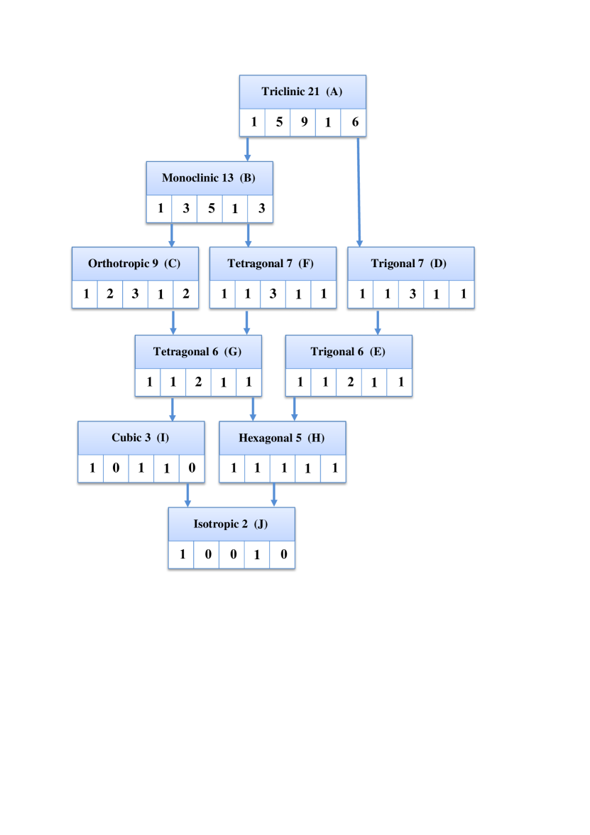
Figure 1: Hierarchy of the symmetry systems. Dimensions of the tensor spaces and of their irreducible parts ${}^{(1)}S^{ijkl}$, ${}^{(2)}S^{ijkl}$, ${}^{(3)}S^{ijkl}$, ${}^{(1)}A^{ijkl}$ and ${}^{(2)}A^{ijkl}$ are indicated.

In order to have a more detailed description of the relation between the symmetry systems, we study now their inclusions and intersections. For briefness, we use now the notations $A,B,\cdots,J$ given in Tab. 1. For two systems connected in Fig. 1 by an arrow, the lower system is included into the higher one. Thus we have obvious inclusions

$$J\subset I\subset G\subset C\subset B\subset A\,,$$ (136)

and so on. We consider now the relations between the system from different branches that are not directly connected one to another by an arrow. First we observe

$$D\cap I=E\cap I=F\cap I=J\,.$$ (137)

Moreover,

$$D\cap H=E\cap H=D\cap G=E\cap G=D\cap C=E\cap C=D\cap B=E\cap B=F$$ (138)

and

$$C\cap G=H$$ (139)

Consequently, we have a diagram in Fig. 2 presented the inclusions of the symmetry systems in the form of Venn’s diagrams from set theory.

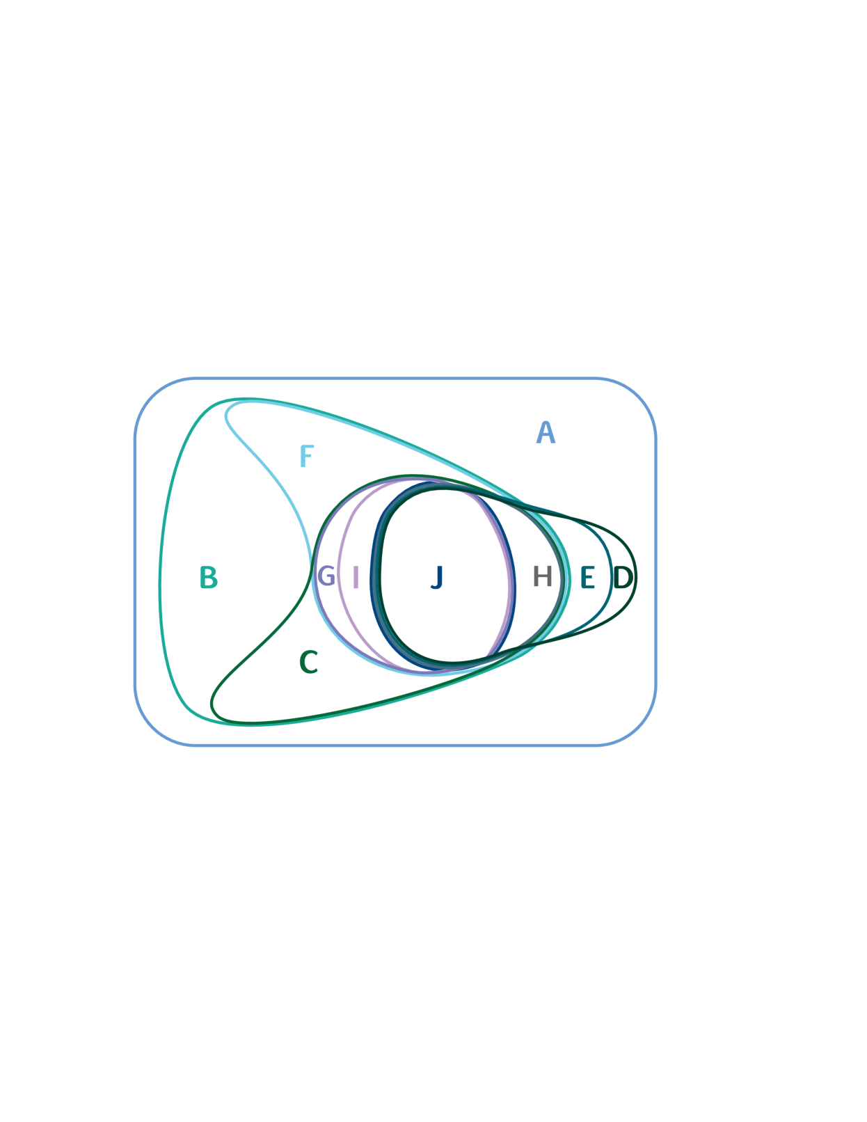
Figure 2: Venn diagrams for inclusion of symmetry systems.

6 Conclusion

In this paper,we presented matrix representations of the elasticity tensor that confirm with its irreducible decompositions. In particular, $(3\times 7)$ matrix corresponds to $GL(3)$ decomposition of the elasicity tensor intoCauchy and non-Cauchy parts. When the traces of the elasticity tensor are applied, an additional $SO(3)$ irreducible decomposition emerges. We describe this decomposition with three $(3\times 3)$ matrices. Two of these matrices are symmetric and one is of a general form. Since the symmetric matrices represent two second order tensors, their traces are extracted in an invariant form and generate two linear invariants of the elasticity tensor.

We apply the irreducible matrix decomposition to all symmetry classes and decompose correspondingly their elasticity tensors. This resolution of the symmetry classes yields a natural scheme of the hierarchy and inclusion of the symmetry classes. This result is in an almost completely correspondence with the diagrams presented in literature.

To our opinion the central problem related to the irreducible decomposition is the physical meaning of the independent pieces. We observe some preliminary results that can be derived from the resolution of the symmetry classes:

• The scalar parts ${}^{(1)}S^{ijkl}$ and ${}^{(1)}A^{ijkl}$ with the scalars $S$ and $A$ enter all symmetry systems. Thus they can be considered as basic states of the deformed material. In particular, the closed isotropic prototype of a material can be derived by extracting these two scalars from the elasticity tensor. In algebraic description it means the orthogonal projection into two one dimensional subspaces, see [18].

• The part ${}^{(3)}S^{ijkl}$ enclosed in all anisotropic crystal systems. Hence its norm can be used as a basic factor of anisotropy. This term, however, enters only the Cauchy part. Thus without additional tensor parts, the non-Cauchy part is left isotropic.

• Two tensor parts ${}^{(2)}S^{ijkl}$ with the tensor $P^{ij}$ and ${}^{(2)}A^{ijkl}$ with the tensor $Q^{ij}$ do not enter only the cubic and the isotropic systems. They can be used as additional characteristics of anisotropy. For trigonal, tetragonal and transverse isotropic systems, these parts are one-dimensional and can be completely described by their norms.

• For the systems with the symmetry higher than orthotropic, an invariant relation between second order tensors holds: the tensors $P^{ij}$ and $Q^{ij}$ are proportional to one another

  $$P^{ij}=CQ^{ij}$$ (140)

  with some numerical coefficient $C$.

References

• [1] Auffray, N., Kolev, B., and Petitot, M. (2014). On anisotropic polynomial relations for the elasticity tensor, Journal of Elasticity, 115, 77-103.
• [2] G. Backus (1970) A geometrical picture of anisotropic elastic tensors, Rev. Geophys. Space Phys. 8, 633–671.
• [3] Baerheim, R. (1993) Harmonic decomposition of the anisotropic elasticity tensor. Quarterly J. Mech. Appl. Math. 46, 391–418.
• [4] Bóna, A., Bucataru, I., & Slawinski, M. A. (2004). Material symmetries of elasticity tensors. Quarterly J. Mech. Appl. Math. 57, 583-598.
• [5] J.D. Clayton, Nonlinear Mechanics of Crystals, Solid Mechanics and Its Applications 177, DOI 10.1007/978-94-007-0350-6, Springer Science+Business Media B.V. 2011
• [6] Cowin, S. C. (1989) Properties of the anisotropic elasticity tensor. Quarterly J. Mech. Appl. Math. 42, 249–266. Corrigenda ibid. (1993) 46, 541–542.
• [7] Cowin, S. C. & Mehrabadi, M. M. (1992) The structure of the linear anisotropic elastic symmetries, J. Mech. Phys. Solids 40, 1459–1471.
• [8] S. C. Cowin and M. M. Mehrabadi (1995) Anisotropic symmetries of linear elasticity, Appl. Mech. Rev., 48(5), 247–285.
• [9] Cowin, S. C. (1995). On the number of distinct elastic constants associated with certain anisotropic elastic symmetries. In Theoretical, Experimental, and Numerical Contributions to the Mechanics of Fluids and Solids (pp. 210-224). Birkhäuser, Basel.
• [10] Fedorov, F. I. (2013) Theory of elastic waves in crystals, Springer Science & Business Media.
• [11] Gazis, D. C., Tadjbakhsh, I., & Toupin, R. A. (1963). The elastic tensor of given symmetry nearest to an anisotropic elastic tensor. Acta Crystallographica, 16 (9), 917-922.
• [12] Haussühl, S. 2007 Physical Properties of Crystals: An Introduction. Weinheim, Germany: Wiley-VCH.
• [13] Hehl, F. W. & Itin, Y. (2002) The Cauchy relations in linear elasticity theory. J. Elasticity, 66, 185–192.
• [14] Forte, S., & Vianello, M. (1998). Functional bases for transversely isotropic and transversely hemitropic invariants of elasticity tensors. Quarterly J. Mech. Appl. Math., 51 (4), 543-552.
• [15] Forte, S.J. Elasticity, & Vianello, M. (1996). Symmetry classes for elasticity tensors. J. Elasticity 43 (2), 81-108.
• [16] Forte, S., & Vianello, M. (2014). A unified approach to invariants of plane elasticity tensors. Meccanica, 49 (9), 2001-2012.
• [17] Itin, Y., & Hehl, F. W. (2013) The constitutive tensor of linear elasticity: Its decompositions, Cauchy relations, null Lagrangians, and wave propagation. J. Math. Phys. 54, 042903.
• [18] Itin, Y. (2016). Quadratic invariants of the elasticity tensor. J. Elasticity 125 (1), 39-62.
• [19] Marsden, J. E. & Hughes, T. J. R. (1983) Mathematical Foundations of Elasticity, Englewood Cliffs, NJ: Prentice-Hall.
• [20] Landau, L. D., & Lifshitz, E. M. (1986). Theory of Elasticity, 3rd. ed: Pergamon Press, Oxford, UK.
• [21] Love, A.E.H., (1920) A treatise on the mathematical theory of elasticity. at the University Press.
• [22] Moakher, M., & Norris, A. N. (2006). The closest elastic tensor of arbitrary symmetry to an elasticity tensor of lower symmetry. J. Elasticity 85, 215-263.
• [23] Norris, A. N. (2007) Quadratic invariants of elastic moduli, Quarterly J. Mech. Appl. Math. 60 (3), 367–389.
• [24] Norris, A.N., (2006) Elastic moduli approximation of higher symmetry for the acoustical properties of an anisotropic material, Journal of Acoustical Society of America 119 (4), 2114-2121
• [25] Nye, J. F. (1985). Physical properties of crystals: their representation by tensors and matrices. Oxford University Press.
• [26] Olive, M., Kolev, B., & Auffray, N. (2017). A minimal integrity basis for the elasticity tensor. Archive for Rational Mechanics and Analysis, 226 (1), 1-31.
• [27] Weber, M., Glüge, R., & Bertram, A. (2018). Distance of a stiffness tetrad to the symmetry classes of linear elasticity. International Journal of Solids and Structures, in press.