Neuromodulated Learning in Deep Neural Networks

Abstract

In the brain, learning signals change over time and synaptic location, and are applied based on the learning history at the synapse, in the complex process of neuromodulation. Learning in artificial neural networks, on the other hand, is shaped by hyper-parameters set before learning starts, which remain static throughout learning, and which are uniform for the entire network. In this work, we propose a method of deep artificial neuromodulation which applies the concepts of biological neuromodulation to stochastic gradient descent. Evolved neuromodulatory dynamics modify learning parameters at each layer in a deep neural network over the course of the network’s training. We show that the same neuromodulatory dynamics can be applied to different models and can scale to new problems not encountered during evolution. Finally, we examine the evolved neuromodulation, showing that evolution found dynamic, location-specific learning strategies.

1 Introduction

In deep learning and machine learning, the learning process is most often cast as an optimization problem of the neural network parameters $\theta$, being synaptic weights and neuron biases, according to some loss function $Q$. In classification, for example, this loss function can be the mean squared error between a target classes, $h_{i}$, and the class given by the deep NN, $X(\theta,i)$:

$$Q_{i}(\theta)=(X(\theta,i)-h_{i})^{2}$$ (1)

$$Q(\theta)=\frac{1}{n}\sum_{i=1}^{n}Q_{i}(\theta)$$ (2)

The standard approach to optimizing the weights $\theta$ of the ANN is to use gradient descent over batches of the data. Classic stochastic gradient descent (SGD) uses a learning rate hyper-parameter, $\eta$ to determine the speed at which weights change based on the loss function. This method can be improved with the addition of momentum [Nesterov, 1983], which changes the weight update based on the previous weight update. An additional hyper-parameter, $\alpha$, is then used to determine the impact of momentum on the final update:

$$\Delta\theta^{(t+1)}\leftarrow\alpha\Delta\theta^{(t)}-\eta\nabla Q_{i}(\theta^{(t)})$$ (3)

$$\theta^{(t+1)}\leftarrow\theta^{(t)}+\Delta\theta^{(t+1)}$$ (4)

In contemporary deep learning, there is a variety of gradient descent approaches to choose from. Adagrad [Duchi et al., 2011] implements an adaptive learning rate and is often used for sparse datasets. Adadelta [Zeiler, 2012] and RMSprop [Tieleman and Hinton, 2018] were both suggested to solve a problem of quickly diminishing learning rates in Adagrad and are now popular choices for timeseries tasks. Adam [Kingma and Ba, 2014] is one of the most widely used optimizers for classification tasks, where past gradients are stored in a variable $m$, and past squared gradients are stored in a variable $v$. Two hyper-parameters, $\beta_{1}$ and $\beta_{2}$, control the update rate of $m$ and $v$, respectively. $m$ and $v$ are then used to update the weights, instead of using the gradient directly. This update has a learning rate hyper-parameter, $\eta$, as well as a “fuzzing factor” hyper-parameter $\epsilon$ which controls the ratio between $m$ and $v$ in the final update.

These methods, as well as others, are all the result of empirical study on specific problems. An overview of their different benefits and weaknesses is presented in [Ruder, 2016], and the choice of optimizer represents an important but difficult decision on the part of the human expert, followed by the equally difficult choice of hyper-parameters for the chosen method. These choices depend on domain, on the data available, on the architecture of the network, and on the training resources available. Furthermore, the choice is restrained to these existing methods, or to the rigorous development of a new optimization method.

In this work, we propose a method to automatically develop an optimizer. Using evolution, a neuromodulatory agent is generated for a training task. This agent, based on artificial gene regulatory networks (AGRN), uses an existing optimizer as a base and modifies the parameters of learning at each layer and at each update. Two different base optimizers were tested: SGD and Adam. We therefore denote the neuromodulatory versions of these optimizers Nm-SGD and Nm-Adam. These optimization bases were chosen based on their popularity for the chosen task, image classification. We use classification on the CIFAR benchmark to demonstrate this method, but it can be applied to any domain, as evolution can create an optimizer specialized for the domain of interest. We show that the evolved neuromodulation strategy can generalize during evolution to different deep ANN architectures and after evolution to a longer training time and to new problems. Furthermore, by analysing the behavior of the evolved AGRN during training, we demonstrate that the location-specific and time-dependent qualities of neuromodulation are important for deep learning training, as they are in the biological brain. This represents a novel foray into location-specific learning for deep neural networks.

2 Background

The field of artificial neuromodulation is in rather new, especially when applied to ANNs. Much of the existing work in this field has focused on reward-based modulation for unsupervised Hebbian learning to allow for supervised learning. In the case of Spike-timing Dependent Plasticity, a type of Hebbian learning based on biological synaptic change, reward-modulated learning has been used in a variety of tasks [Frémaux and Gerstner, 2016]. In [Farries and Fairhall, 2007], a spiking neural network was trained using neuromodulated STDP to elicit specific spike train. Similarly, in [Izhikevich, 2007], a population response of neurons firing in a specific group was demonstrated, using a model of neuromodulation based on a chemical dopamine signal.

A non-spiking example of neuromodulated Hebbian learning is in in [Velez and Clune, 2017], where diffusion-based neuromodulation is used to eliminate catastrophic forgetting in ANNs. The ANNs used in this work are shallow networks trained using Hebbian learning to perform multiple tasks.

Artificial neuromodulation has also been studied in other contexts than ANNs. In [Harrington et al., 2013], a robot agent learns to cover an area in a reinforcement learning scheme. The agent is trained by SARSA, which is itself controlled by an evolved neuromodulator. This work was extended in [Cussat-Blanc and Harrington, 2015], where evolved neuromodulation agents facilitate multi-task learning. This work also uses SARSA as the agent.

The task of artificial neuromodulation can be seen as part of the “learning to learn” or “meta-learning” problem of optimizing the learning process. Active learning optimization of this nature has been the topic of much study, such as in [Andrychowicz et al., 2016], where a secondary ANN is introduced to optimize the learning of the primary network. In [Miconi et al., 2018], additional Hebbian learning is shown to improve the performance of networks trained through gradient descent.

Our focus in this work is to evolve the rules of neuromodulation, using two existing learning methods, SGD and Adam, as a base and improving upon these methods with evolution. The physical aspects of the neural network are central to the design of the neuromodulation controller. SGD is traditionally a global process, with a static learning rate used for all neurons. While methods like [Kingma and Ba, 2014] offer dynamic learning rates, these rates are applied throughout the network. In the brain, the location of a neuron highly impacts its learning. Neuromodulation often employs volume transmission as a means of communicating, using chemicals to distribute information as opposed to synaptic or wired transmission [Agnati et al., 2010]. Clusters of neurons physically concentrated together will share chemical signals, even if they have disparate connections. Some neuromodulatory signals are wide-ranged, effecting entire sections of neurons together, while others are highly localized, modulating learning in only a few neurons.

The neuromodulation controllers were also designed to be responsive, changing over time and in response to neural activity. In the brain, this is an important aspect of learning, where neuromodulation is itself controlled by activity in the brain. In [Pignatelli and Bonci, 2015], the role of synaptic plasticity of dopaminergic neurons is examined, showing that external pressures such as stress can change the behavior of these neurons. The response of a synapse to dopamine changes also over time and depends on the state of the neuron.

The goal of the evolved controllers is therefore to use information about the neurons, i.e. their placement, activity, and learning history, to modify learning as it happens and in different ways across the network. For this purpose, we evolve an artificial controller, an AGRN, to regulate the parameters of learning at each layer. AGRNs, a model based on biological gene regulatory networks, have been shown to be capable evolved agents on a number of tasks, including signal processing, robot navigation, and game playing [Disset et al., 2017]. In the next section, we present the AGRN model for neuromodulation.

3 AGRN neuromodulation model

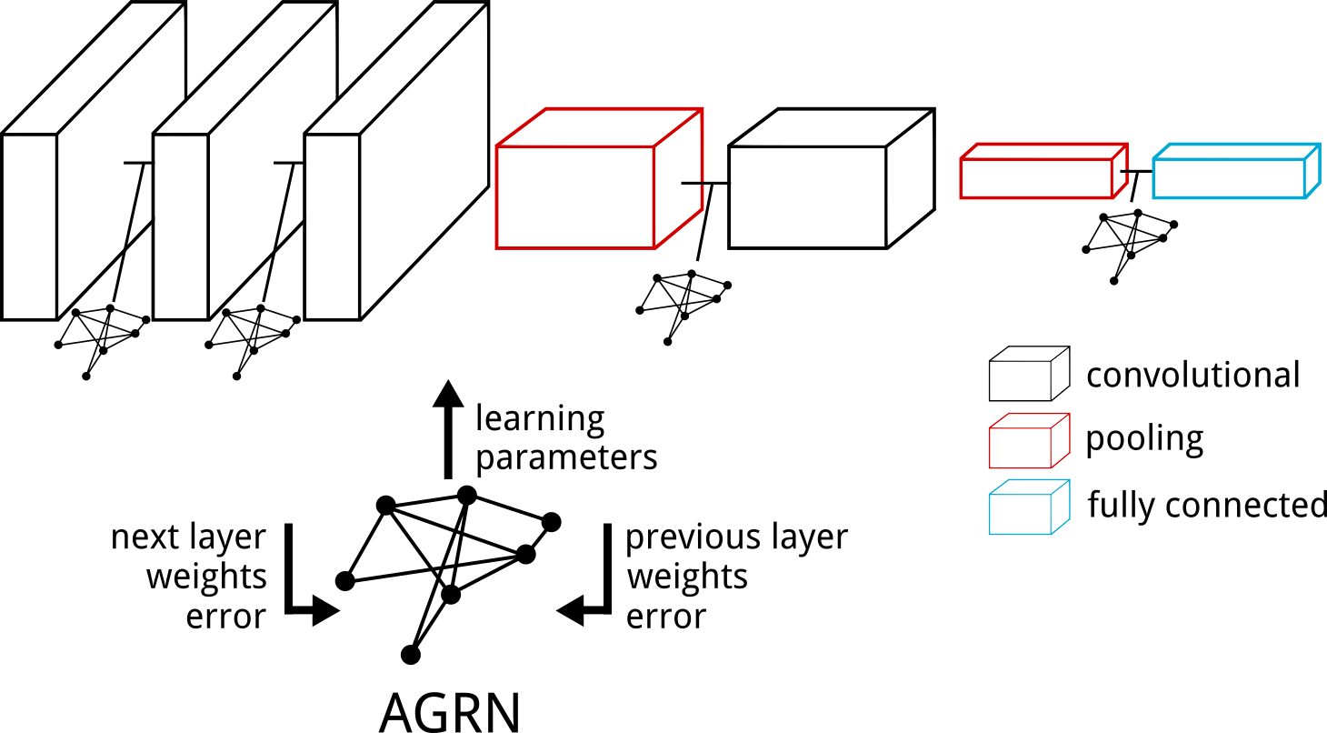
Figure 1: The neuromodulation architecture. A copy of the evolved AGRN is placed between all weighted layers of the network. Inputs are given to the AGRN at each batch update with information about the two layers between which the AGRN is placed. The AGRN then outputs the learning parameters to be used in that batch update for the first of the two layers.

The neuromodulation architecture consists of AGRNs placed between all layers of a deep neural network where weights and gradients are defined (pooling layers, for example, do not have a corresponding AGRN). The parameters of learning in the first of the two layers surrounding each AGRN are decided by the AGRN. The AGRN receives information about the two layers surrounding it, and about the weights and gradients in both layers. The neuromodulation computation happens in three steps: 1) collecting the appropriate inputs, 2) processing these through the AGRN, and 3) using the outputs as learning parameters. This computation takes place at each update step, i.e. at the end of each batch, which we refer to as one iteration. In the neuromodulation architecture, each AGRN has the same genetic code, which is found by evolution; different behavior from the different AGRN copies arises due to the different inputs given at each layer. A separate AGRN is used for the synaptic weights and neuron biases of each layer, so there are two AGRN copies for each layer. All layers except pooling layers use biases.

The inputs of each AGRN consist of static information about the layer, i.e. its location and size, and statistical information about the weights and gradients, i.e. the mean and standard deviation of both. To be processed by the AGRN, each input must be between 0.0 and 1.0, so different normalization methods or constraints are used. For the layer location input, each deep ANN layer is given a location index $l$ from 0, the first layer, to $L$, the last layer, and the input is input is $l/L$. The layer size input is similarly normalized over the entire ANN; the size of each layer, being the number of parameters in the layer, is divided by the number of parameters of the largest layer in the network. The statistical information is not normalized but instead constrained in $[0.0,1.0]$. The absolute value of the weights are used for the mean and standard deviation inputs, $\mu_{\theta}$ and $\sigma_{\theta}$, based on the observation that the magnitude of the weights rarely exceed 1.0. Similarly, the absolute value of the gradients was used to calculate $\mu_{\nabla Q}$ and $\sigma_{\nabla Q}$.

These six inputs, layer location, $\mu_{\theta}$, $\sigma_{\theta}$, $\mu_{\nabla Q}$, $\sigma_{\nabla Q}$, and layer size, are found for each layer. The AGRN receives the inputs of the layer before and after it, making 12 inputs. An additional 13th input is also included; this input provides constant activation of 1.0. This was included to mitigate the possible case that, for certain layers, none of the inputs would have a high enough magnitude to provide sufficient activation of the regulatory proteins of the AGRN.

The outputs of the AGRN are the hyper-parameters of the relevant optimizer. For Nm-SGD, the outputs are the learning rate, $\eta$, and the momentum parameter $\alpha$. For Nm-Adam, the outputs are the two $\beta$ parameters, $\beta_{1}$ and $\beta_{2}$, $\epsilon$, and the learning rate $\eta$. The full list of inputs and outputs are given in Table 1.

Inputs	SGD output	Adam output
layer location	$\eta$	$\eta$
$\mu_{\theta}$	$\alpha$	$\beta_{1}$
$\sigma_{\theta}$		$\beta_{2}$
$\mu_{\nabla Q}$		$\epsilon$
$\sigma_{\nabla Q}$
layer size

Table 1: The layer inputs and hyper-parameter outputs of the AGRN. All inputs are specific to a layer, and the AGRN receives two copies of these inputs, one for each layer surrounding the AGRN. With the constant activation input, there are 13 total input proteins. For each output parameter, two AGRN output proteins are used. There are therefore 4 output proteins for SGD and 8 output proteins for Adam.

In the standard AGRN update step, protein concentrations are normalized to sum to 1. This is a part of AGRN computation that has been shown to be necessary [Disset et al., 2017], but it can have the undesirable consequence of restraining the protein concentration levels. In order to allow the AGRNs to control the magnitude of its outputs, irrespective of normalization, two output proteins are assigned to each learning hyper-parameter. The normalized difference between the two output protein concentrations, $o$, is then used to compute the hyper-parameter output, $O$:

$$O_{i}=\frac{|o_{2i}-o_{2i+1}|}{o_{2i}+o_{2i+1}}$$ (5)

The AGRN used in Nm-SGD therefore has 13 input proteins and 4 output proteins, and for Nm-Adam it has 13 input proteins and 8 output proteins. These two different neuromodulation schemes present two different optimization problems; to find an AGRN, with the respective number of inputs and outputs, capable of improving overall learning of a deep ANN by making local changes to the learning parameters at each layer. In the next section, we describe the use of artificial evolution to find the neuromodulatory AGRNs.

4 Evolution of the neuromodulatory agent

The evolutionary method used in this work is GRNEAT, a genetic algorithm specialized in AGRN evolution [Cussat-Blanc et al., 2015]. A key component of using GRNEAT, or any genetic algorithm, is the design of the evolutionary fitness function used for selection. In this work, we aim to find an AGRN which improves learning. Specifically, we use each AGRN individual during training for the same number of epochs, $E=20$ and then compare these individuals based on their accuracy on the trained task. In order to ensure generalization, we modify the deep ANN model and random initialization seed at each generation.

The task used for training during evolution is CIFAR-10 [Krizhevsky and Hinton, 2009]. This is a standard image classification task where 60000 32x32 color images are presented from 10 classes, with 6000 images per class. We chose this benchmark due to its prevalence in the literature and for the ease of testing a more difficult problem, CIFAR-100, without needing to change deep ANN models or the data infrastructure. CIFAR-100 is the same size as CIFAR-10, but has 100 classes containing 600 images each. Results on the CIFAR-100 benchmark are presented in section 6.

At each generation during evolution, a deep ANN model is chosen. This model is used to evaluate all individuals in the generation, providing a standard platform for comparison. We use three different models, $m0$, $m1$, and $m2$, which are presented in Table 2. These models were based on popular image classification architectures (LeNet and VGG16) and were chosen to evaluate neuromodulation on a variety of model sizes, from the small $m0$, which is unable to solve CIFAR-10, to the complex $m2$. The choice of model during evolution is random; one of the three models is chosen per generation according to a uniform distribution.

$m0$	$m1$	$m2$
conv 32	conv 64	conv 64
conv 32	maxpool	maxpool
maxpool	conv 128	conv 128
conv 64	maxpool	maxpool
conv 64	conv 256	conv 256
maxpool	maxpool	maxpool
fc 512	conv 512	conv 512
fc $n_{out}$	maxpool	maxpool
	fc 4096	conv 512
	fc 4096	maxpool
	fc $n_{out}$	fc 4096
		fc 4096
		fc $n_{out}$

Table 2: The three models used during evolution, $m0$, $m1$, and $m2$. Layer types are convolutional (conv), maxpool, and fully connected (fc), with the size of the layer indicated. $n_{out}$ is the number of outputs and depends on problem; for CIFAR-10, used during evolution, $n_{out}=10$.

Each AGRN individual is therefore used to train a deep ANN, of one of the three architectures, on the CIFAR-10 dataset, which is split into training and testing sets of 50000 and 10000 images, respectively. The evolutionary fitness used was the training accuracy at the end of the final epoch. This metric was chosen to avoid giving the AGRN an advantage from export to the test data.

Nm-SGD and Nm-Adam agents were evolved using GRNEAT. For the next sections, we selected the best individuals from 50th generation of each evolution, one for Nm-SGD and one for Nm-Adam. These two individuals were used to compare neuromodulation to the base optimization methods in the next section.

5 Comparison of neuromodulation to standard optimization

Using the best individual from the last generation of the evolution for Nm-SGD and Nm-Adam, we compare neuromodulation with standard methods. We first compare them on the evolutionary task, CIFAR-10. For SGD and Adam, we compare against the default parameters of the Keras framework, as well as parameters found through a grid search. These parameters are presented in Table 3, with the “decay” parameter being the learning rate decay over each update.

method	model	$\eta$	$\alpha$	decay
SGD	all	0.01	0.0	0.0
SGD*	$m0$	0.01	0.75	0.0
	$m1$	0.1	0.0	0.001
	$m2$	0.01	0.5	0.0

method	model	$\eta$	$\beta_{1}$	$\beta_{2}$	$\epsilon$	decay
Adam	all	0.001	0.9	0.999	$10^{-}8$	0.0
Adam*	$m0$	0.001	0.9	0.999	0.001	0.0
	$m1$	0.1	0.99	0.9	1.0	0.001
	$m2$	0.1	0.99	0.999	1.0	0.001

Table 3: Keras default parameters for the two base methods, and the parameters found through search. To find the optimal parameters, all parameter combinations over defined ranges were tried, and the best parameter set was selected based on final training accuracy on the CIFAR-10 set.

We trained the three different models using the compared optimizers 10 times each. This was done to ensure fair comparison with different random initial weights. The results of the comparison on training accuracy are presented in Figure 2.

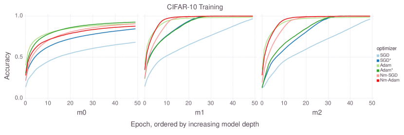
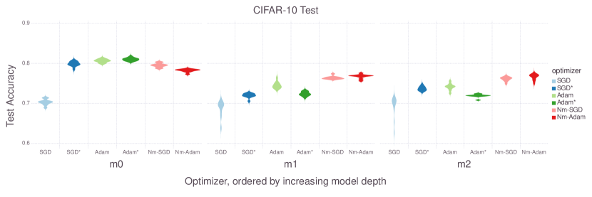
Figure 2: Training and test accuracy on the CIFAR-10 benchmark of the neuromodulatory methods, Nm-SGD and Nm-Adam, compared to the base methods.

First, we observe that the neuromodulation methods, Nm-SGD and Nm-Adam, are able to generalize to longer training times. These methods were evolved for 20 epochs, but are here trained for 50 epochs. Especially when training on the model $m0$, we can see that Nm-SGD and Nm-Adam both continue to aid training after 20 epochs.

We can also see that neuromodulation can limit overfitting. While the training accuracy achieved by Nm-SGD and Nm-Adam are both very near 1.0 by the end of 50 epochs on $m1$ and $m2$, the test accuracy for both methods on these models is superior to that of either standard SGD or Adam.

Finally, we see that the neuromodulatory training can converge faster than standard training, seen especially for models $m1$ and $m2$. This may be a result of the use of 20 epochs in the evolutionary fitness, as convergence speed wasn’t explicitly selected for. Instead, by evaluating AGRNs after 20 epochs, those that converged early may have presented an evolutionary benefit.

6 Generalization of the neuromodulatory agent

Next, we compare these four optimization methods on the CIFAR-100 benchmark. The experiment is the same, i.e. the three different models are trained in 10 separate trials, but the dataset is different and 100 epochs are used to account for the more difficult dataset. CIFAR-100 is a challenging change from CIFAR-10. The number of classes increases from 10 to 100, and the number of examples from each class decreases from 6000 to 600 (5000 to 500 in the training set). The network must therefore be trained on sparser data for more classes. This new task would often present the need to find new hyper-parameters, requiring an expensive tuning search. Here, we use the AGRNs evolved on CIFAR-10 to test their generalization to CIFAR-100 without change. The results from this experiment are presented in Figure 3.

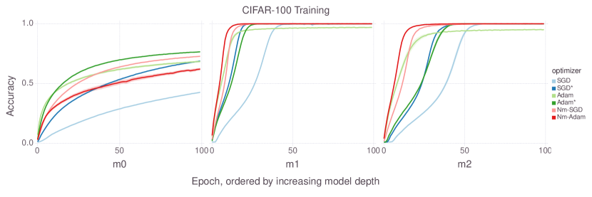
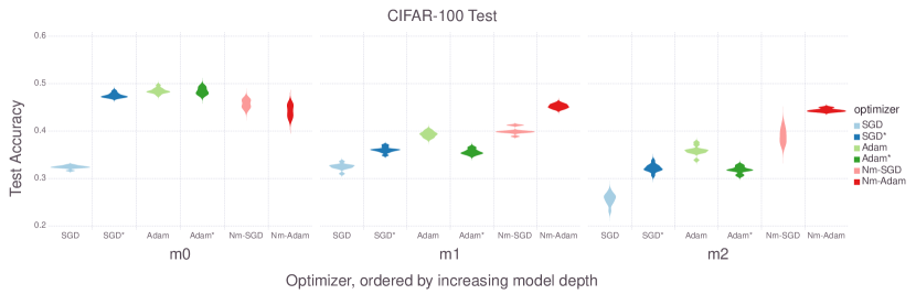
Figure 3: Training and test accuracy on the CIFAR-100 benchmark of the neuromodulatory methods, Nm-SGD and Nm-Adam, compared to their base methods, SGD and Adam.

Nm-SGD and Nm-Adam show clear capabilities to adapt to this new task, outperforming the base methods on $m1$ and $m2$, while producing early equivalent test results on $m0$. The training accuracy on $m0$ of Nm-SGD is the highest of the methods tried, but Nm-Adam is lower than standard Adam. It is possible that the chosen individual for Nm-Adam was not as suited to the smallest architecture $m0$ as others from the same evolution, due to the random selection of model during evolution. Nm-Adam does perform well across the different models, with better training and test accuracy than the model-specific Adam* methods.

The conclusions drawn from the CIFAR-10 experiments hold for CIFAR-100. Both neuromodulation methods exhibit an ability to generalize to longer training, here extending from 20 epochs during evolution to 100 epochs here. The test accuracy, especially of Nm-Adam, remains high across different models and is better than that of SGD and Adam for $m1$ and $m2$. It is worth nothing that the evolutionary fitness was only related to the training accuracy, and on the simpler CIFAR-10 set. There was no evolutionary pressure towards generalization to other problems nor to avoiding overfitting, yet the evolved neuromodulation dynamics are capable of both.

These experiments demonstrate the viability of this method. Evolved AGRNs can make effective hyper-parameter choices at each layer, leading to optimized learning. We now examine the behavior of the AGRNs to understand this function and the hyper-parameters chosen.

7 Neuromodulation behavior

To understand the behavior of the evolved AGRN, we observe the inputs and outputs of each AGRN copy during training. Specifically, we present the Nm-Adam CIFAR-10 training of $m1$. This training is shorter than CIFAR-100 and involves fewer AGRN copies than $m2$. We evaluate a single training, not the training over 10 different initial weight conditions, as presented in the previous sections. These choices were made to allow the results to be better understood, as the inputs and outputs of each AGRN over training represents a large amount of data, while providing an interesting use-case, the Nm-Adam training on $m1$. The training is presented in iterations, which are the update steps at each batch. The batch size used in all experiments was 128, meaning there were 391 iterations per epoch and a total of 19550 iterations over 50 epochs.

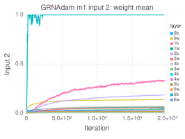
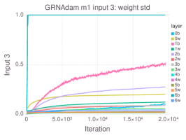
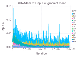
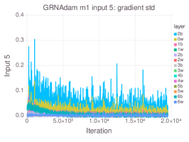
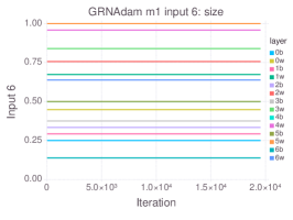
Figure 4: Input protein concentrations during Nm-Adam training on $m1$, with each AGRN copy represented by a different color. Layer names indicate either neuron bias, “b”, or synaptic weight, “w”.

We first present the inputs given to each AGRN in Figure 4. We show only the first six inputs, as this contains all of the relevant information. The next six inputs of each AGRN are the same values for the next layer, already represented in the shown inputs. The final input, the constant activation input, is always 1.0 for all layers.

The surprising aspect of these inputs is that the biases of the final layer do exceed 1.0 after a small amount of training. This restricts the information the AGRN is able to receive about these weights, as $\mu_{\theta}$ is constrained to 1.0. We also see that the gradient mean, $\mu{\nabla Q}$ is generally very small and could potentially be scaled when provided as an input for easier use by the AGRN. Finally, while the gradient provides noisy oscillations, most inputs are static throughout the training, especially after the halfway point of 1e4 iterations.

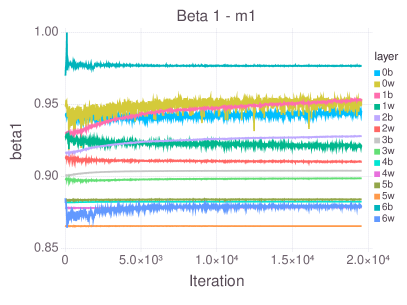
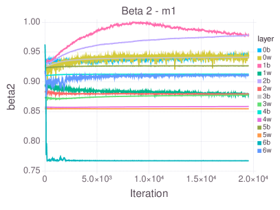
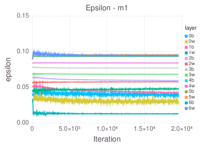
Figure 5: The hyper-parameters chosen during Nm-Adam training on $m1$, with each AGRN copy represented by a different color. Layer names indicate either neuron bias, “b”, or synaptic weight, “w”.

The hyper-parameters decided by the AGRN are presented in Figure 5. For this evolved AGRN individual, it is clear that there is a nearly direct relationship between $\mu_{\theta}$ and $\eta$ for the biases in the last layer, as the learning rate mirrors the bias mean almost exactly. There are notable differences in the early layers, however, with the learning rate of the weights of layer 0 displaying an inverse relationship with $\mu_{\theta}$. This is an example of a location-specific neuromodulation strategy, a behavior which is not possible with standard optimization methods.

Most hyper-parameters are static over time, or like the training, stabilize after 1e4 iterations. The $\beta_{2}$ parameter of the biases of layer 1 is an exception to this, decreasing during the second half of training. This means that, near the middle of the training, the update of $v_{\theta}$ depends almost entirely on its previous state and not on the squared gradient. It only changes based on the squared gradient at the beginning and ends of training. While this behavior was not common for the hyper-parameter choices, this sort of variability over time is a known aspect of neuromodulation and is also not possible using standard optimization methods.

8 Conclusion

In this work, we found that artificially neuromodulated optimizers improved learning on standard classification benchmarks. Furthermore, neuromodulatory dynamics were discovered that improve learning on previously unseen problems. As these dynamics were discovered automatically through evolution, this method of artificial neuromodulation can be applied to any situation where learning task performance can be ranked for evolutionary selection.

We believe that this method could lead to shared improvements for deep learning. At the end of evolution, a single AGRN individual is selected from the entire population, across all generations. In this work, this was the best individual from the final population. However, a single evolution creates a wealth of different individuals, which can be selected based on other characteristics, like their size. We have shown that a single individual can generalize to longer training and new problems without needing more training. We can therefore imagine that neuromodulatory agents could be shared, much as trained neural networks are shared, with agents evolved for certain task types and architectures, i.e. image classification. As in the case of “model zoos”, a repository of neuromodulatory agents could be shared, eliminating the need to choose hyper-parameters and improving optimization.

Artificial neuromodulation is a promising direction for deep meta-learning. Principles of biological neuromodulation were shown in this work to play an important role in learning. Local signals which change over time were used to decide the rate of learning and the importance of other factors, such as momentum, in weight change. These dynamics are novel for stochastic gradient descent methods, and we believe these characteristics of learning could lead to the design of new optimization methods.

References

- [Agnati et al., 2010] Agnati, L. F., Guidolin, D., Guescini, M., Genedani, S., and Fuxe, K. (2010). Understanding wiring and volume transmission. Brain research reviews, 64(1):137–159.
- [Andrychowicz et al., 2016] Andrychowicz, M., Denil, M., Gomez, S., Hoffman, M. W., Pfau, D., Schaul, T., Shillingford, B., and De Freitas, N. (2016). Learning to learn by gradient descent by gradient descent. In Advances in Neural Information Processing Systems, pages 3981–3989.
- [Cussat-Blanc and Harrington, 2015] Cussat-Blanc, S. and Harrington, K. (2015). Genetically-regulated Neuromodulation Facilitates Multi-Task Reinforcement Learning. In Proceedings of the 2015 on Genetic and Evolutionary Computation Conference - GECCO ’15, pages 551–558, New York, New York, USA. ACM Press.
- [Cussat-Blanc et al., 2015] Cussat-Blanc, S., Harrington, K., and Pollack, J. (2015). Gene regulatory network evolution through augmenting topologies. IEEE Transactions on Evolutionary Computation, 19(6):823–837.
- [Disset et al., 2017] Disset, J., Wilson, D. G., Cussat-Blanc, S., Sanchez, S., Luga, H., and Duthen, Y. (2017). A comparison of genetic regulatory network dynamics and encoding. In Proceedings of the Genetic and Evolutionary Computation Conference, pages 91–98. ACM.
- [Duchi et al., 2011] Duchi, J., Hazan, E., and Singer, Y. (2011). Adaptive subgradient methods for online learning and stochastic optimization. Journal of Machine Learning Research, 12(Jul):2121–2159.
- [Farries and Fairhall, 2007] Farries, M. A. and Fairhall, A. L. (2007). Reinforcement Learning With Modulated Spike Timing-Dependent Synaptic Plasticity. Journal of neurophysiology, 98(6):3648–3665.
- [Frémaux and Gerstner, 2016] Frémaux, N. and Gerstner, W. (2016). Neuromodulated Spike-Timing-Dependent Plasticity, and Theory of Three-Factor Learning Rules. Frontiers in Neural Circuits, 9(January).
- [Harrington et al., 2013] Harrington, K. I., Awa, E., Cussat-Blanc, S., and Pollack, J. (2013). Robot Coverage Control by Evolved Neuromodulation. In Angelov, P., Levine, D., and Erdi, P., editors, The 2013 International Joint Conference on Neural Networks, pages 1–8, Piscataway, NJ, USA. IEEE.
- [Izhikevich, 2007] Izhikevich, E. M. (2007). Solving the distal reward problem through linkage of STDP and dopamine signaling. Cerebral Cortex, 17(10):2443–2452.
- [Kingma and Ba, 2014] Kingma, D. P. and Ba, J. (2014). Adam: A method for stochastic optimization. arXiv preprint arXiv:1412.6980.
- [Krizhevsky and Hinton, 2009] Krizhevsky, A. and Hinton, G. (2009). Learning multiple layers of features from tiny images. Technical report, Citeseer.
- [Miconi et al., 2018] Miconi, T., Clune, J., and Stanley, K. O. (2018). Differentiable plasticity: training plastic neural networks with backpropagation. arXiv preprint arXiv:1804.02464.
- [Nesterov, 1983] Nesterov, Y. E. (1983). A method for solving the convex programming problem with convergence rate O(1/k). In Dokl. Akad. Nauk SSSR, volume 269, pages 543–547.
- [Pignatelli and Bonci, 2015] Pignatelli, M. and Bonci, A. (2015). Role of Dopamine Neurons in Reward and Aversion: A Synaptic Plasticity Perspective. Neuron, 86(5):1145–1157.
- [Ruder, 2016] Ruder, S. (2016). An overview of gradient descent optimization algorithms. CoRR, abs/1609.04747.
- [Tieleman and Hinton, 2018] Tieleman, T. and Hinton, G. (2018). Divide the gradient by a running average of its recent magnitude.
- [Velez and Clune, 2017] Velez, R. and Clune, J. (2017). Diffusion-based neuromodulation can eliminate catastrophic forgetting in simple neural networks. PloS one, 12(11):e0187736.
- [Zeiler, 2012] Zeiler, M. D. (2012). ADADELTA: an adaptive learning rate method. arXiv preprint arXiv:1212.5701.