A practical light transport system model for chemiluminescence distribution reconstruction

Abstract

Plenoptic cameras and other integral photography instruments capture richer angular information from a scene than traditional 2D cameras. This extra information is used to estimate depth, perform superresolution or reconstruct 3D information from the scene. Many of these applications involve solving a large-scale numerical optimization problem. Most published approaches model the camera(s) using pre-computed matrices that require large amounts of memory and are not well-suited to modern many-core processors. We propose a flexible camera model based on light transport and use it to model plenoptic and traditional cameras. We implement the proposed model on a GPU and use it to reconstruct simulated and real 3D chemiluminescence distributions (flames) from images taken by traditional and plenoptic cameras.

I Introduction

Plenoptic cameras [9, 10], cameras with coded masks [11], and other integral photography equipment augment traditional 2D photographic measurements with additional angular information. They do this by interposing additional lenses, masks or other elements along the optical path from the scene to the detector; these additional provide angular information about the scene that is “integrated away” by traditional cameras. The spatial/angular data acquired by one of these devices can facilitate depth estimation, digital refocusing, superresolution, and, in the main application of this paper, tomographic reconstruction of chemilumiscence distributions, i.e., flames.

The 3D structure of translucent luminescent objects is relevant for multiple mechanical engineering and modeling tasks [12, 13, 14]. Previous works have used multiple traditional or plenoptic cameras to acquire enough angular information to reconstruct the object [15, 16]. This is often done by numerically solving an inverse problem, and a key part of that problem is the model that predicts from a candidate 3D chemiluminescence distribution, ${\bm{x}}$, the resulting image on a camera, ${\bm{A}}{\bm{x}}$. Although these works have taken different approaches to modeling the physics of the acquisition process, the most common practice has been to precompute the (sparse but large) matrix ${\bm{A}}$ and use sparse linear algebra routines to solve the reconstruction problem. While this technique can produce good results, it is computationally expensive and solving even relatively small problems can take many hours even using GPU linear algebra libraries, in part because computing speed gains have outpaced memory bandwidth increases in modern many-core computing systems.

This work proposes a practical light transport-based framework for the camera model, ${\bm{A}}$. Instead of precomputing the system matrix ${\bm{A}}$, we provide expressions to compute its entries on the fly, which is significantly more efficient. We then describe an efficient GPU implementation. The system is “light transport-based” in the sense that it numerically implements a discrete version of certain analytical light transport techniques [17, 18] to analyze camera properties. This structure results in camera models that are compositions of simple light transport steps; this enables modeling a wide range of camera designs with only a few tools. We present results quantifying the accuracy of the proposed system model and apply it to several image reconstruction problems with simulated and real data. Mathematically, the chemiluminescence reconstruction problem is similar to SPECT image reconstruction [19, 20]; in both cases the goal is to reconstruct the spatial distribution of the rate of emission of photons using models for the system physics. Unlike traditional SPECT, the chemiluminescence reconstruction problem we consider gathers information only from a few fixed camera positions, and therefore has relatively sparse angular information about the object.

Section II describes how we implement the light transport “building block” operations. Section III models 3D chemiluminescence distributions. Section IV discusses some implementation practicalities, Section V proposes a multi-camera reconstruction algorithm for a chemiluminescence distribution, and Section VI contains some experiments. Section VII contains some concluding remarks.

II Camera system model

This section derives computational models for the progression of light from a scene to the camera’s detector. The main tool we use is light transport via geometric optics. The model describes how an incident light field propagates stage-by-stage through the camera to the detector. To accomplish this, we discretize (i.e., define a finite-series representation of) the light field at each stage spatially (e.g., on the detector along pixel boundaries) and angularly (by where the described light field passes through a designated “angular plane.”). The resulting model is highly parallelizable and has computationally efficient forward and transpose operations (those operations are essential for use in many inverse problem settings).

II-A Geometric optics

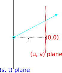
Figure 1: Two-plane ray parameterization

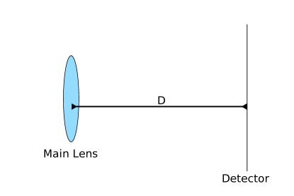
Figure 2: Schematic of a single-lens camera

In this paper we model light transport using geometric optics, following earlier works, e.g., [18, 17]. Because we are interested in modeling the behavior of cameras imaging scenes at macro scale, we do not need to resort to wave transport [21] to model the imaging process. This section summarizes the elements of light transport used in the proposed system model.

The monochrome light field function defined at a given plane at a fixed time is a four dimensional real-valued function $\mathsf{L}:\mathbb{R}^{4}\to\mathbb{R}$. The light field function has two spatial arguments ${\left(s,t\right)}$ and two angular arguments ${\left(u,v\right)}$, using the common two-plane parameterization [22]; see Figure 1. Together these coordinates $\bm{\theta}={\left(s,u,t,v\right)}$ describe the position and angular orientation of a ray passing through the light field’s $(s,t)$ plane. The corresponding value of the light field function at that point gives the radiance along that ray.

TABLE I: Common affine optical transformations

Operation	Transformation
Propagation by $d$	$\bm{T}_{d}{\left(\bm{\theta}\right)}={\left[\begin{matrix}1&d&0&0\\ 0&1&0&0\\ 0&0&1&d\\ 0&0&0&1\end{matrix}\right]}{\left[\begin{matrix}s\\ u\\ t\\ v\end{matrix}\right]}$
Thin lens refraction with focal length $f$ and center ${{\left(s,t\right)}={\left(s_{0},t_{0}\right)}}$	$\bm{R}_{f}{\left(\bm{\theta}\right)}={\left[\begin{matrix}1&0&0&0\\ -1/f&1&0&0\\ 0&0&1&0\\ 0&0&-1/f&1\end{matrix}\right]}{\left[\begin{matrix}s\\ u\\ t\\ v\end{matrix}\right]}$
	$\hskip 150.00023pt+{\left[\begin{matrix}0\\ s_{0}/f\\ 0\\ t_{0}/f\end{matrix}\right]}$

Geometric optics describes how rays of light are altered, i.e., how the parameters $\bm{\theta}$ change, as rays pass through space and refracting media; including, particularly for this paper, ideal thin lenses and occluding masks. Ignoring diffraction and attenuation, light transport corresponds to transformations of $\bm{\theta}$ that are affine and easy to compute. Table I gives expressions for the transformations used in this paper.

The expressions in Table I are composed to describe more complex optical effects. For example, a ray $\bm{\theta}$ entering the camera in Figure 2 is refracted by the main lens, then travels the distance $D$ before landing on the detector. That is, the light field on the detector, $\mathsf{L}^{\text{det}}{\left(\bm{\theta}\right)}$, is determined by the light field impinging on the main lens, $\mathsf{L}^{\text{main}}{\left(\bm{\theta}\right)}$:

$$\mathsf{L}^{\text{main}}{\left(\bm{\theta}\right)} =\mathsf{L}^{\text{det}}{\left({\bm{X}}^{\text{det-main}}{\left(\bm{\theta}\right)}\right)},$$ (1)

where ${\bm{X}}^{\text{det-main}}{\left(\bm{\theta}\right)}={\left(\bm{T}_{D}\circ\bm{R}_{f_{\text{main}}}\right)}{\left(\bm{\theta}\right)},$ and $\circ$ denotes function composition. For any two planes $p$ and $q$ in an optical system, we use the notation $\bm{X}^{pq}$ to describe the optical transformation from $q$ to $p$.

Because we will refer to specific entries of such optical transformations later in this paper, we denote any such the optical transformation $\bm{X}$ as

$${\left[\begin{matrix}X_{\mathrm{s}}{\left(\bm{\theta}\right)}\\ X_{\mathrm{u}}{\left(\bm{\theta}\right)}\\ X_{\mathrm{t}}{\left(\bm{\theta}\right)}\\ X_{\mathrm{v}}{\left(\bm{\theta}\right)}\end{matrix}\right]} ={\left[\begin{matrix}X_{\mathrm{ss}}&X_{\mathrm{su}}&0&0\\ X_{\mathrm{us}}&X_{\mathrm{uu}}&0&0\\ 0&0&X_{\mathrm{tt}}&X_{\mathrm{tv}}\\ 0&0&X_{\mathrm{vt}}&X_{\mathrm{vv}}\\ \end{matrix}\right]}{\left[\begin{matrix}s\\ u\\ t\\ v\end{matrix}\right]}+{\left[\begin{matrix}\overline{X}_{\mathrm{s}}\\ \overline{X}_{\mathrm{u}}\\ \overline{X}_{\mathrm{t}}\\ \overline{X}_{\mathrm{v}}\end{matrix}\right]}.$$ (2)

The separable structure follows from the ideal geometric optics in Table I and helps yield convenient computational structures. It is possible to extend the work in this paper to handle non-separable optical transformations, and one could use the transformation factorization approach described in Section III-A to implement many non-separable transformations efficiently.

II-B Light field discretization

Consider a plane normal to the primary axis of the optical system. To store and compute the light field at that plane, we approximate it with a basis expansion, as is common in other inverse problems [23, 24]. Light field $\mathsf{L}{\left(\bm{\theta}\right)}$ has two spatial and two angular variables; we discretize the spatial dimension $(s,t)$ using separable pillbox functions, i.e., pixels. To handle the angular coordinates $(u,v)$, we designate a plane in the optical system and discretize the light field by where the ray $\bm{\theta}$ lands on that plane. Often, but not always, this plane is along the main lens of the camera. We call this plane the “angular plane” of the system. In our approach, all light fields in the optical system use the same angular plane for angular discretization.

Let ${\bm{X}}^{0p}$ denote the optical transformation from the plane $p$ (including all lenses and free-space propagation) to the selected angular plane. We represent the light field at the plane $p$ using the following basis expansion with coefficients ${\bm{f}}^{p}\in\mathbb{R}^{N^{p}K}$:

$$\mathsf{L}^{p}{\left(\bm{\theta};{\bm{f}}^{p}\right)} =\sum_{k=1}^{K}a{\left(\frac{X^{0p}_{\mathrm{s}}{\left(s,u\right)}-s_{k}}{\Delta_{\mathrm{s}}^{0}}\right)}a{\left(\frac{X^{0p}_{\mathrm{t}}{\left(t,v\right)}-t_{k}}{\Delta_{\mathrm{t}}^{0}}\right)}$$

$$\times\sum_{i=1}^{N^{p}}b{\left(\frac{s-s_{i}}{\Delta_{\mathrm{s}}^{p}}\right)}b{\left(\frac{t-t_{i}}{\Delta_{\mathrm{t}}^{p}}\right)}f^{p}_{ki},$$ (3)

where $N^{p}$ denotes the number of pixels and $K$ denotes the number of angular coordinate samples (sub-aperture images). The basis center points ${\left\{{\left(s_{k},t_{k}\right)}\right\}}$ on the angular plane and, (lightly recycling notation) ${\left\{{\left(s_{i},t_{i}\right)}\right\}}$ on the plane $p$, are separated by the respective distances ${\left\{{\left(\Delta_{\mathrm{s}}^{0},\Delta_{\mathrm{t}}^{0}\right)}\right\}}$ and ${\left\{{\left(\Delta_{\mathrm{s}}^{p},\Delta_{\mathrm{t}}^{p}\right)}\right\}}$, respectively. The spatial basis function $b{\left(\cdot\right)}$ is the standard rectangular function:

$$b{\left(t\right)} =\begin{cases}1,&{\left|t\right|}\leq\frac{1}{2}\\ 0,&\text{else.}\end{cases}$$ (4)

We consider two choices for the basis function on the angular plane, $a{\left(\cdot\right)}$: the rect function $b$, that leads to a 2D “pillbox” basis, and the Dirac impulse $\delta$. Using $a=\delta$ yields slightly simpler expressions in Section II-C for light transport, but we found that it often requires a finer (and therefore more computationally expensive) discretization of the angular plane to produce an accurate model. The Dirac impulse basis is used implicitly when a finite camera lens is modeled as a superposition of pinhole cameras [25]. Section VI-A explores this trade-off.

II-C Light transport

Let $p$ and $q$ be two planes in the optical system with the same optical plane. Assume that $q$ is closer to the scene and $p$ is closer to the detector; to model the camera’s image acquisition process, we model the transport from $q$ to $p$.

The optical transformations from $q$ and $p$ to the angular plane are $\bm{X}^{0q}$ and $\bm{X}^{0p}$, respectively. From these expressions, the optical transformation from $q$ to $p$ is $\bm{\theta}^{p}=\bm{X}^{pq}{\left(\bm{\theta}^{q}\right)}$ where $\bm{X}^{pq}={{\left[\bm{X}^{0p}\right]}^{-1}\circ\bm{X}^{0q}}$. In general, when we start with a light field having the representation (3), after a transformation it will no longer have exactly that same representation. This property is acceptable since (3) is already an approximation of the continuous light field. To maintain (3) as a consistent form of the representation throughout the model, after each optical transformation we project the transformed light field onto a finite dimensional subspace of the form (3). Specifically, to find the coefficients of the discrete light field on $p$, ${\bm{f}}^{p}$, from the coefficients of the light field on $q$, ${\bm{f}}^{q}$, we solve the following optimization problem in $L_{2}{\left(\mathbb{R}^{4}\right)}$:

$${\bm{f}}^{p} =\mathop{\text{argmin }}_{{\bm{f}}}{\left|\left|\mathsf{L}^{p}{\left(\bm{X}^{pq}{\left(\cdot\right)};{\bm{f}}\right)}-\mathsf{L}^{q}{\left(\cdot;{\bm{f}}^{q}\right)}\right|\right|}_{2}^{2}.$$ (5)

This least-squares approximation problem has a block-separable solution with $K$ blocks, ${\bm{f}}^{p}={\left({\bm{f}}^{p}_{1},\ldots,{\bm{f}}^{p}_{K}\right)}$; one block for each basis function on the angular plane:

$${\bm{f}}^{p}_{k}=\frac{1}{V^{p}}\bm{B}^{pq}_{k}{\bm{f}}^{q}_{k},$$ (6)

where the “volume” of a basis element in $\mathbb{R}^{4}$ on plane $p$ is defined by

$$V^{p}={\left|\left|a{\left(\frac{X^{0p}_{\mathrm{s}}{\left(s,u\right)}}{\Delta_{\mathrm{s}}^{0}}\right)}a{\left(\frac{X^{0p}_{\mathrm{t}}{\left(t,v\right)}}{\Delta_{\mathrm{t}}^{0}}\right)}b{\left(\frac{s}{\Delta_{\mathrm{s}}^{p}}\right)}b{\left(\frac{t}{\Delta_{\mathrm{t}}^{p}}\right)}\right|\right|}_{2}^{2}.$$ (7)

The entries of $\bm{B}^{pq}_{k}$ come from the ${\left(s,t,u,v\right)}$ inner products:

$${\left[\bm{B}^{pq}_{k}\right]}_{ij} =\left<b{\left(\frac{X^{pq}_{\mathrm{s}}{\left(s,u\right)}-s_{i}}{\Delta_{\mathrm{s}}^{p}}\right)}a{\left(\frac{X^{0q}_{\mathrm{s}}{\left(s,u\right)}-s_{k}}{\Delta_{\mathrm{s}}^{0}}\right)},\right.$$

$$\left.\hskip 40.00006ptb{\left(\frac{s-s_{j}}{\Delta_{\mathrm{s}}^{q}}\right)}\right>\times$$

$$\hskip 11.00008pt\left<b{\left(\frac{X^{pq}_{\mathrm{t}}{\left(t,v\right)}-t_{i}}{\Delta_{\mathrm{t}}^{p}}\right)}a{\left(\frac{X^{0q}_{\mathrm{t}}{\left(t,v\right)}-t_{k}}{\Delta_{\mathrm{t}}^{0}}\right)},\right.$$

$$\left.\hskip 40.00006ptb{\left(\frac{t-t_{j}}{\Delta_{\mathrm{t}}^{q}}\right)}\right>,$$ (8)

where the first inner product is over $${\left(s,u\right)} {\left(t,v\right)}$$ and the second is over . After some simplification,

$${\left[\bm{B}^{pq}_{k}\right]}_{ij} =\int_{s_{j}-\Delta_{\mathrm{s}}/2}^{s_{j}+\Delta_{\mathrm{s}}/2}h_{k,\mathrm{s}}^{pq}g{\left(s-\alpha^{pq}_{k,\mathrm{s}}s_{i};\bm{\tau}^{pq}_{k,\mathrm{s}}\right)}~{}\text{d}s$$

$$\hskip 30.00005pt\times\int_{t_{j}-\Delta_{\mathrm{t}}/2}^{t_{j}+\Delta_{\mathrm{t}}/2}h_{k,\mathrm{t}}^{pq}g{\left(t-\alpha^{pq}_{k,\mathrm{t}}t_{i};\bm{\tau}^{pq}_{k,\mathrm{t}}\right)}~{}\text{d}t.$$ (9)

The blur kernel $g$ results from an inner integral over $u$ or $v$ and depends on the choice of angular basis function $a$. The magnification terms ${\left\{\alpha^{pq}_{k,*}\right\}}$ and blur parameters ${\left\{\bm{\tau}^{pq}_{k,*}\right\}}$ depend only on the planes $p$ and $q$ and the angle $k$. For the Dirac $\delta$ and pillbox angular basis functions, the blur integrals and blur parameters are efficient to derive and compute. Tables II and III give expressions for these parameters for the $s$ direction; the $t$ direction expressions are analogous.

TABLE II: Dirac basis transport expressions

Property	Expression
Blur kernel	$g{\left(s\right)}=\begin{cases}1,&\tau_{s1}^{pqk}\leq w<\tau_{s2}^{pqk}\\ 0,&\text{else.}\end{cases}$
	$\alpha=X^{pq}_{\mathrm{ss}}-X^{0q}_{\mathrm{ss}}X^{pq}_{\mathrm{su}}/X^{0q}_{\mathrm{su}}$
	$\beta=\overline{X}^{pq}_{\mathrm{s}}+X^{pq}_{\mathrm{su}}{\left(s_{k}-\overline{X}^{0q}_{\mathrm{s}}\right)}/X^{0q}_{\mathrm{su}}$
	$\widehat{}\bm{\tau}_{s}^{pqk}={\left(\pm\Delta_{\mathrm{s}}^{p}/2-\beta\right)}/\alpha$
Blur parameters	$\bm{\tau}_{s}^{pqk}=\text{sort-ascend}{\left\{\widehat{}\bm{\tau}_{s}^{pqk}\right\}}$
Blur height	$h^{pqk}_{s}=\Delta^{0}_{s}/{\left|X^{0q}_{\mathrm{su}}\right|}$
Blur magnification	$\alpha^{pqk}_{s}=1/\alpha$
Basis element volume	$V^{p}=\Delta_{\mathrm{s}}^{p}\Delta_{\mathrm{t}}^{p}{\left|\Delta_{\mathrm{s}}^{0}\Delta_{\mathrm{t}}^{0}/{\left(X^{0p}_{\mathrm{su}}X^{0p}_{\mathrm{tv}}\right)}\right|}$

TABLE III: Pillbox basis transport expressions

Property	Expression
Blur kernel	$g{\left(s\right)}=\begin{cases}\frac{s-\tau_{s1}^{pqk}}{\tau_{s2}^{pqk}-\tau_{s1}^{pqk}},&\tau_{s1}^{pqk}\leq s<\tau_{s2}^{pqk};\\ 1,&\tau_{s2}^{pqk}\leq s<\tau_{s3}^{pqk};\\ 1-\frac{s-\tau_{s3}^{pqk}}{\tau_{s4}^{pqk}-\tau_{s3}^{pqk}}&\tau_{s3}^{pqk}\leq s<\tau_{s4}^{pqk};\\ 0&\text{else.}\end{cases}$
	$\alpha=X^{pq}_{\mathrm{ss}}-X^{pq}_{\mathrm{su}}X^{0q}_{\mathrm{ss}}/X^{0q}_{\mathrm{su}}$
	$\beta=X^{pq}_{\mathrm{su}}/X^{0q}_{\mathrm{su}}$
	$\gamma=\overline{X}^{pq}_{\mathrm{s}}-X^{pq}_{\mathrm{su}}\overline{X}^{0q}_{\mathrm{s}}/X^{0q}_{\mathrm{su}}$
	$\widehat{}\bm{\tau}_{s}^{pqk}={\left(\pm\Delta_{\mathrm{s}}^{p}/2-\beta{\left(s_{k}\mp\Delta_{\mathrm{s}}^{0}/2\right)}-\gamma\right)}/\alpha$
Blur parameters	$\bm{\tau}_{s}^{pqk}=\text{sort-ascend}{\left\{\widehat{}\bm{\tau}_{s}^{pqk}\right\}}$
Blur height	$\mathop{\text{min}}{\left\{{\left|\Delta_{\mathrm{s}}^{0}/X^{0q}_{\mathrm{su}}\right|},{\left|\Delta_{\mathrm{s}}^{p}/X^{pqk}_{\mathrm{su}}\right|}\right\}}$
Blur magnification	$\alpha_{s}^{pqk}=1/\alpha$
	$m_{\mathrm{s}}=\text{max}{\left\{\Delta_{\mathrm{s}}^{0}/2{\left|X^{0p}_{\mathrm{su}}\right|},\Delta_{\mathrm{s}}^{p}{\left|X^{0p}_{\mathrm{ss}}/X^{0p}_{\mathrm{su}}\right|}/2\right\}}$
	$h_{s}=\text{min}{\left\{\Delta_{\mathrm{s}}^{p},\Delta_{\mathrm{s}}^{0}/{\left|X^{0p}_{\mathrm{ss}}\right|}\right\}}$
	$V^{p}_{s}=2m_{s}h_{s}$
Basis element volume	$V^{p}=V^{p}_{s}V^{p}_{t}$

Note that the entries of $\bm{B}^{pq}_{k}$ are separable products of one-dimensional $s$ and $t$ functions (9). Consequently, we implement $\bm{B}^{pq}_{k}$ as the Kronecker product

$$\bm{B}^{pq}_{k}=\bm{B}^{pq}_{k\mathrm{s}}\otimes\bm{B}^{pq}_{k\mathrm{t}}.$$ (10)

II-D Occlusion

The final important optical elements we need to model are occluders, e.g., a coded mask inside the camera [11] or outside the lens [26]. For an occluder on the plane $p$, let $\mathsf{L}^{p-}$ be the light field at $p$ on the side of the occluder towards the scene and $\mathsf{L}^{p+}$ be the light field at $p$ on the side towards the detector. We model occlusion in terms of the light field coefficients as

$${\bm{f}}_{k}^{p+} =\bm{M}{\bm{f}}_{k}^{p-},$$ (11)

where $\bm{M}$ is a $N^{p}\times N^{p}$ diagonal matrix that encodes the occluder’s spatial behavior. We compute the entries of $\bm{M}$ by rasterizing the occluder’s support onto the spatial grid for $\mathsf{L}^{p}$.

II-E Measurement formation

Let $\mathsf{L}^{d}$ be the light field on the detector, and we choose the spatial discretization of $\mathsf{L}^{d}$ to align with the spatial discretization of the detector. In the absence of noise, the $i$th sensor measurement is the integral of the irradiance of the light over the spatial extent of the $i$th sensor cell, and with this choice of discretization the integral simplifies as follows:

$$y_{i} =\int_{s\in S_{i}}\int_{t\in T_{i}}\int_{u\in\mathbb{R}}\int_{v\in\mathbb{R}}\mathsf{L}^{d}{\left(s,u,t,v\right)}~{}\text{d}s~{}\text{d}u~{}\text{d}t~{}\text{d}v$$

$$=\sqrt{V^{d}}\sum_{k=1}^{K}f^{d}_{ki}.$$ (12)

Thus the vector of measurements ${\bm{y}}$ is simply the sum over each angular component

$${\bm{y}} =\sqrt{V_{d}}\sum_{k=1}^{K}{\bm{f}}_{k}^{d}.$$ (13)

II-F Camera models

We combine the operations in the preceding sections to model single-lens and plenoptic cameras. For both types of cameras, we place the angular plane on the main lens, and consider transporting a scene light field $\mathsf{L}^{s}$, parameterized by ${\bm{f}}^{s}$ located $D_{\text{scene}}$ units from the camera’s main lens to the detector plane. The optical transformation from $\mathsf{L}^{s}$ to the angular plane is $\bm{X}^{0s}={\left(\bm{T}_{D_{\text{scene}}}\circ\bm{R}_{f_{\text{main}}}\right)}^{-1}$, where $\bm{R}_{f\text{main}}$ denotes refraction by the main lens.

II-F1 Single lens camera

Modeling a single lens camera, Figure 2, requires a single transport operation, from the scene light field $\mathsf{L}^{s}$ through the main lens to the detector light field $\mathsf{L}^{d}$. The optical transformation from the detector to the angular plane is the propagation $\bm{X}^{0d}=\bm{T}_{D}$, where $D$ is the distance from the detector to the main lens. With $\bm{X}^{0d}$ and $\bm{X}^{0s}$ defined, we can follow Sections II-C and II-E to write the single lens camera system model:

$${\bm{y}}_{\text{single}} =\sqrt{V^{d}}\sum_{k=1}\bm{B}^{ds}_{k}{\bm{f}}^{s}_{k}.$$ (14)

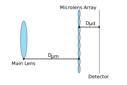
Figure 3: Schematic of a plenoptic camera

II-F2 Plenoptic camera

In a plenoptic camera, light from the main lens falls on an array of microlenses that further refract the light onto the detector; see Figure 3. We model this configuration using two stages: an initial transport onto the microlens array, followed by masking and transport through each of the microlenses onto the detector.

Let $D_{\mu\text{m}}$ be the distance between the microlens array and the main lens. The optical transformation from the microlens array (prior to refraction through the microlenses) is the propagation $\bm{X}^{0a}=\bm{T}_{D_{\mu m}}$; let $\bm{B}^{as}$ denote the transport operation from the scene $\mathsf{L}^{s}$ to the microlens array. Not all the light incident on the microlens array will be refracted onto the detector; we assume that light falling between microlenses is occluded. We model this with a diagonal masking matrix $\bm{M}$ (11).

The light field incident on the detector, $\mathsf{L}^{d}$ is the superposition of the light that is refracted through each of the $N_{\mu}$ microlenses; i.e., $\mathsf{L}^{d}{\left(\cdot\right)}=\sum_{\mu=1}^{N_{\mu}}\mathsf{L}^{\mu}{\left(\cdot\right)}$. The optical transformation from behind each microlens to the angular plane is unique, because each microlens has a different center location (and possibly different optical parameters): $\bm{X}^{0\mu}={\bm{X}}^{0a}\circ\bm{R}_{\mu}\circ\bm{T}_{D_{d\mu}}$.

Combining the first transport onto the microlens array, masking, and microlens transport yields the following (noiseless) plenoptic camera measurement model:

$${\bm{y}}_{\text{plenoptic}} =\sum_{k=1}^{K}{\left[\sum_{\mu=1}^{N_{\mu}}\sqrt{V^{\mu}}\bm{B}^{d\mu}_{k}\right]}{\bm{M}}\bm{B}^{\mu s}_{k}{\bm{f}}^{s}_{k}.$$ (15)

III Chemiluminescence object model

One application of the computational transport model described above is reconstructing a 3D chemiluminescence distribution from images captured by several cameras. We model the continuous monochrome chemiluminscence distribution $f$ using a 3D array of voxels; i.e., products of pillbox functions in the $x$, $y$ and $z$ directions:

$$f{\left(x,y,z\right)} =\sum_{j=1}^{N}b{\left(\frac{x-\widetilde{x}_{j}}{\Delta_{\mathrm{x}}}\right)}b{\left(\frac{y-\widetilde{y}_{j}}{\Delta_{\mathrm{y}}}\right)}b{\left(\frac{z-\widetilde{z}_{j}}{\Delta_{\mathrm{z}}}\right)}x_{j},$$ (16)

where ${\left\{x_{j}\right\}}$ are the coefficients of the expansion and ${\left\{{\left(\widetilde{x}_{j},\widetilde{y}_{j},\widetilde{z}_{j}\right)}\right\}}$ are the voxel centers. To simplify the acquisition model for a single camera, we assume initially that the object’s $x$, $y$ and $z$ directions are parallel to the camera’s $s$, $t$ and axial directions, respectively. Section III-A describes the generalization for rotated objects.

We assume that the only source of light in the scene is the chemiluminescent body $f$, and there are no reflecting objects in the camera’s field of view. Consequently, the radiance along each ray through the scene depends on a line integral through $f$.

With the object and camera coordinate systems aligned, it is convenient to view the object $f$ as a set of $N_{\mathrm{z}}$ “slices”, each corresponding to a different value of the axial coordinate $z$. We “collapse” each slice into a light field at the center of each slice using a small-angle approximation, and use the light transport tools in the previous section to model the acquisition process. Let $\mathsf{L}^{s}$ be the light field originating from the slice $z=z_{s}$, defined with respect to the camera’s angular plane, with vector expansion coefficients ${\bm{w}}^{s}_{k}=\Delta_{\mathrm{z}}{\bm{x}}^{s}$, and $\bm{C}^{ds}$ be the camera measurement operator from $\mathsf{L}^{s}$ onto the camera’s detector (as described in the previous section). The image acquisition model is

$${\bm{y}}=\sum_{s=1}^{N_{\mathrm{z}}}\bm{C}^{ds}{\bm{w}}^{s}.$$ (17)

For some camera models, it is computationally efficient to factor common terms of the camera operators ${\left\{\bm{C}^{ds}\right\}}_{s=1}^{N_{z}}$. For example, we factor the plenoptic camera measurement model into two steps: propagation of each light field view from every slice onto the microlens array, followed by propagation through the microlens array:

$${\bm{y}}_{\text{plenoptic}} =\sum_{k=1}^{K}\underbrace{{\left[\sum_{\mu=1}^{N_{\mu}}\sqrt{V^{\mu}}\bm{B}^{d\mu}_{k}\right]}{\bm{M}}}_{\text{array onto detector}}\underbrace{{\left[\sum_{s=1}^{N_{\mathrm{z}}}\bm{B}^{\mu s}_{k}{\bm{w}}^{s}_{k}\right]}}_{\text{scene onto array}}.$$ (18)

An unfactorized implementation of the plenoptic camera model would require $O{\left(N_{\mathrm{z}}N_{\mu}K\right)}$ transport operations; this factorization (18) reduces that to $O{\left(K{\left(N_{\mathrm{z}}+N_{\mu}\right)}\right)}$.

III-A Rotated perspectives

For most multiple-camera or multiple-perspective acquisitions, it is unlikely that the coordinate systems of each camera and the single object $f$ will be aligned. Consequently, we need to be able to image $f$ from a rotated perspective as well as from the simpler “head-on” perspective in the previous section. Our approach resamples $f$ and its “natural” coefficients ${\bm{x}}$ into a rotated coordinate system with coefficients ${\bm{p}}^{\mathrm{r}}$ for the rotated perspective. The imaging model for each rotated camera is the composition of the camera model and the rotation operators.

We take an approach similar to the classical three-pass technique used in image rotation [27, 28]. Similar to those works, we consider rotations along each axis of less than $45$ degrees; larger rotations can be modeled as a composition of a permutation operation (i.e., rotation by $n$ $90$ degree rotations) and a smaller rotation.

Let ${\bm{p}}\in\mathbb{R}^{3}$ be a point in the object’s “natural” coordinate system and ${\bm{p}}^{\mathrm{r}}$ be the same point in the rotated coordinate system: ${\bm{p}}={\bm{\Theta}}{\bm{p}}^{\mathrm{r}}$, where ${\bm{\Theta}}$ is a $3\times 3$ rotation matrix. This matrix can be decomposed as a composition of a diagonal matrix, ${\bm{D}}_{\bm{\Theta}}$ and three shear coordinate transformations:

$${\bm{\Theta}} ={\bm{D}}_{\bm{\Theta}}\bm{S}_{\mathrm{z}}\bm{S}_{\mathrm{x}}\bm{S}_{\mathrm{y}},$$ (19)

where ${\bm{D}}_{\bm{\Theta}}=\mathop{\text{diag}}{\left\{D_{\mathrm{x}},~{}D_{\mathrm{y}},~{}D_{\mathrm{z}}\right\}}$ and e.g.,

$$\bm{S}_{z} ={\left[\begin{matrix}1&0&0\\ 0&1&0\\ S_{\mathrm{zx}}&S_{\mathrm{zy}}&1\end{matrix}\right]}.$$ (20)

We implement 3D rotation by applying each of these coordinate transforms serially, i.e., from left to right in (19). Each of the operations is motivated by functional approximation, as in [27] and in (5). The first operation, scaling the coordinates with the diagonal matrix ${\bm{D}}_{\bm{\Theta}}$, simply changes the voxel sizes:

$$\Delta_{x}^{r}=\frac{\Delta_{\mathrm{x}}}{D_{\mathrm{x}}},\quad\Delta_{y}^{r}=\frac{\Delta_{\mathrm{y}}}{D_{\mathrm{y}}},\quad\Delta_{z}^{r}=\frac{\Delta_{\mathrm{z}}}{D_{\mathrm{z}}}.$$ (21)

Unlike rotation methods that merely involve interpolation [27, 28], we we want to maintain the basis representation (16) even after rotation. Thus, to determine the coefficients ${\bm{r}}^{z}$ after, say, the $z$ shear transform from the original coefficients ${\bm{x}}$, we perform a least-squares projection similar to that in (5) as follows:

$${\bm{r}}^{z} =\mathop{\text{argmin }}_{\bm{r}}{\left|\left|f{\left(\bm{S}_{\mathrm{z}}{\left(\cdot\right)};{\bm{r}}\right)}-f{\left(\cdot;{\bm{x}}\right)}\right|\right|}$$

$$={\bm{E}}^{\mathrm{z}}{\bm{x}},$$ (22)

where the norm is from $L_{2}{\left(\mathbb{R}^{3}\right)}$ and $f{\left(x,y,z;{\bm{x}}\right)}$ is parameterized with the new voxel sizes (16). In a similar way, we compute ${\bm{r}}^{x}$ from ${\bm{r}}^{z}$ and so on: ${\bm{x}}^{r}={\bm{E}}^{\mathrm{y}}{\bm{E}}^{\mathrm{x}}{\bm{E}}^{\mathrm{z}}{\bm{x}}$.

III-A1 Shear transformations

The shear transformations ${\bm{E}}^{\mathrm{x}}$, ${\bm{E}}^{\mathrm{y}}$ and ${\bm{E}}^{\mathrm{z}}$ are block-diagonal with Toeplitz blocks. That is, in each transformation, for all the non-sheared directions (e.g., for ${\bm{E}}^{\mathrm{x}}$, for the range of entries with the same ${\left(y,z\right)}$ coordinates), the transformation is Toeplitz. The operations also shear only in one direction; i.e., the operators have block structure, e.g.,

$${\left[{\bm{E}}^{\mathrm{z}}\right]}_{ij} =\begin{cases}\int_{z\in Z_{j}}g^{\mathrm{z}}{\left(z-z_{i}-\alpha^{x_{i}y_{i}}\right)}\text{~{}d}z,&x_{i}=x_{j},y_{i}=y_{j}\\ 0,&\text{else.}\end{cases}$$ (23)

The interpolation function $g^{\mathrm{z}}$ is a piecewise quadratic function and is derived using the same techniques as the light transport expressions in Section II. Again, we evaluate the elements of ${\bm{E}}^{\mathrm{z}}$ on the fly rather than precomputing and storing them as sparse matrices to accelerate computation on modern many-core hardware.

III-B System models

All the operations in this section are linear so their composition is also linear. For the sake of brevity, we use ${\bm{A}}:\mathbb{R}^{N}\to\mathbb{R}^{M}$ to denote the composition of operators that represents the action of a camera that produces an $M$-pixel image from an $N$-voxel chemiluminescence distribution.

IV Practical implementation

The previous two sections describe the system model that relates the unknown chemiluminescence expansion coefficients ${\bm{x}}$ to the camera measurements ${\bm{y}}$. These expressions could be used to precompute the measurement matrix for a camera, ${\bm{A}}$, that, with the algorithm in Section V, could be used to estimate ${\bm{x}}$ from the measurements ${\bm{y}}$. This is the most common approach in the literature [15, 29, 30, 16], and although it would produce the same results as our proposed method, the reconstruction would be extremely time-consuming, even with GPU-accelerated sparse linear algebra libraries.

In X-ray CT [31] and other time-sensitive inverse problems, this approach is impractical. Instead, the entries of ${\bm{A}}$ are computed on-the-fly by routines that compute the projection (${\bm{A}}{\bm{x}}$) and backprojection (${\bm{A}}^{\intercal}{\bm{y}}$) matrix-vector products. In this section, we describe how we implement these operations efficiently using a GPU for chemiluminescence imaging.

GPUs can execute effectively thousands of “threads” simultaneously. A common programming model (e.g., used by both CUDA and OpenCL) defines an N-dimensional integer lattice and launches a “thread” for each point in the lattice. The threads are separated into groups that execute in SIMD (single instruction multiple data) if possible; i.e., the threads execute simultaneously provided the threads are executing the same instruction (e.g., “add” or “multiply”) albeit on different data. If two threads in the same group execute different instructions, the group of threads serially executes each different execution path; this is called “thread divergence.” To maximize throughput, thread divergence should be avoided as much as possible.

Memory accesses have a similar property. A group of threads can read or write simultaneously from the GPU’s memory provided the addresses they access are adjacent (although more modern GPUs relax this requirement); these are called “coalesced” memory accesses. More irregular memory access patterns result in serialized memory accesses, reducing parallelism.

Finally, to avoid data races or speed-decreasing locking mechanisms, we assign at most one thread to each coordinate of an output vector. That is, when computing the light transport ${\bm{f}}^{p}_{k}=\bm{B}^{pq}_{k}{\bm{f}}^{q}_{k}$, only one thread writes to each element of ${\bm{f}}^{p}_{k}$.

IV-A Adjoint operations

Sections II and III derive expressions for rows of matrices representing the light transport and rotation operations. This is convenient for implementing the forward operations, e.g., $\bm{B}^{pq}_{k}{\bm{f}}^{q}_{k}$, because the elements of $\bm{B}^{pq}_{k}$ needed by the $i$th thread to compute ${\left[\bm{B}^{pq}_{k}{\bm{f}}^{q}_{k}\right]}_{i}={\left[{\left(\bm{B}^{pq}\right)}_{k}^{\intercal}\right]}_{i}^{\intercal}{\bm{f}}^{q}_{k}$ are readily available. However, it may be less immediately obvious how to compute the adjoints needed for the gradient-based optimization method we use in Section V. In some applications, e.g., X-ray CT, some system models may have a parsimonious representation for either its rows or columns but not both [31]. Fortunately, the $L_{2}$ approximation framework (5) used here leads to equally efficient adjoints. For example, the light transport operation (5) has adjoint

$$\frac{1}{V^{p}}{\left(\bm{B}^{pq}\right)}^{\intercal}{\bm{f}}^{p}=\frac{1}{V^{p}}\bm{B}^{qp}{\bm{f}}^{p}=\frac{V^{q}}{V^{p}}\underbrace{{\left(\frac{1}{V_{q}}\bm{B}^{qp}{\bm{f}}^{p}\right)}}_{\text{Transport from $p$ to $q$}},$$ (24)

due to the $p,q$ symmetry of the inner product definition of $\bm{B}^{pq}$ (8); i.e., $\bm{B}^{pq}={\left(\bm{B}^{qp}\right)}^{\intercal}$. All the non-diagonal operations in this paper share this property, so to implement a fast adjoint we only need a scaled version of a fast forward implementation.

IV-B Nondiverging coalesced filtering

The core operation in our models for both light transport and volume rotation is separable Toeplitz-like (10) or Toeplitz (23) filtering. Using separability, we decompose these operations into two (or three, for rotation) operations. Although this strategy requires additional kernels to be launched, which incurs some overhead, the composition-based implementation can reduce computation significantly. For example, the separable implementation requires $O{\left(T+S\right)}$ operations instead of $O{\left(ST\right)}$ operations per pixel, where $S$ and $T$ are the widths in pixels of the $s$ and $t$ blurs, respectively.

We store the light field view at the plane $p$ as a $N_{\mathrm{s}}^{p}\times N_{\mathrm{t}}^{p}$ column-major matrix, i.e., the $s$ dimension varies most quickly in memory.

TABLE IV: Kernels for light transport

Name	Operation	Input order	Output order
Minor filtering	Filter in $t$ direction	$N_{\mathrm{s}}^{q}\times N_{\mathrm{t}}^{q}$	$N_{\mathrm{t}}^{p}\times N_{\mathrm{s}}^{q}$
Major filtering	Filter in $s$ direction	$N_{\mathrm{t}}^{p}\times N_{\mathrm{s}}^{q}$	$N_{\mathrm{s}}^{p}\times N_{\mathrm{t}}^{p}$

Table IV lists the kernels that perform the light transport operation $\bm{B}^{pq}_{k}$. We first filter in the $t$ (minor) direction. We do this because filtering in the data’s major direction would lead to either thread divergence or noncoalesced memory accesses, since computing integrals over disjoint regions of the blur functions (8, 23), often involves diverging operations. After filtering, each group of threads transposes the data using local memory before writing it to a temporary vector. The transpose places $s$ in the minor direction, and we repeat the operation, again ending with a transpose using local memory to return the data to the original ordering.

V Reconstruction algorithm

Suppose we have $N_{\mathrm{c}}$ monochrome cameras with corresponding system models ${\left\{{\bm{A}}_{c}\right\}}$ that acquire images of the chemiluminescence distribution ${\left\{{\bm{y}}_{c}\right\}}$, where

$${\bm{y}}_{c} ={\bm{A}}_{c}{\bm{x}}+{\bm{\varepsilon}}_{c},$$ (25)

where ${\bm{\varepsilon}}_{c}$ denotes the measurement noise for the $c$th camera. We assume that the geometrical configuration of the cameras with respect to the object is known (which often requires calibration). Our goal is to estimate $\widehat{}{\bm{x}}\in\mathbb{R}^{N}$, the vector of basis expansion coefficients for the chemiluminescence distribution.

Because we may be acquiring data from different types of cameras with different ADCs and other properties, we do not assume that we know the relative gains of each of the cameras and will need to estimate them. Since the rate of photon emission from each voxel via chemiluminescence is nonnegative, we constrain $\widehat{}{\bm{x}}$ to be nonnegative. This leads to the following penalized nonnegative least squares problem:

$$\Psi{\left({\bm{x}},{\left\{\gamma_{c}\right\}}\right)} =\frac{1}{2}{\left|\left|{\bm{A}}_{1}{\bm{x}}-{\bm{y}}_{1}\right|\right|}_{\bm{W}_{1}}^{2}+\sum_{c=2}^{N_{\mathrm{c}}}\frac{1}{2}{\left|\left|{\bm{A}}_{c}{\bm{x}}-\gamma_{c}{\bm{y}}_{c}\right|\right|}_{\bm{W}_{c}}^{2}$$

$$\hskip 80.00012pt+\nu{\left|\left|{\bm{x}}\right|\right|}_{1}+\mathsf{R}{\left({\bm{x}}\right)}$$

$$\widehat{}{\bm{x}} =\mathop{\text{argmin }}_{{\bm{x}}\geq{\bm{0}}}\mathop{\text{min}}_{{\left\{\gamma_{c}\right\}}}\Psi{\left({\bm{x}},{\left\{\gamma_{c}\right\}}\right)},$$ (26)

where $\gamma_{c}$ is the unknown gain for the $c$th camera. To avoid degeneracy, we assume the gain for the first camera is unity, without loss of generality. The nonnegative diagonal weights matrix $\bm{W}_{c}$ is used to, e.g., select a Bayer pattern of pixels or disregard a damaged region of the detector. In low-light situations, $\bm{W}_{c}$ could also be used to approximate the combination of the Poisson photon statistics with the Gaussian electronic readout noise [32, 33]. The differentiable and convex edge-preserving regularizer $\mathsf{R}$ encourages piecewise smoothness in $\widehat{}{\bm{x}}$ by penalizing the differences between adjacent voxels:

$$\mathsf{R}{\left({\bm{x}}\right)} =\frac{\beta}{2}\sum_{j=1}^{N}\sum_{l\in\mathcal{N}_{j}}\psi{\left(x_{j}-x_{l}\right)},$$ (27)

where $\mathcal{N}_{j}$ contains the 26 3D neighbors of the $j$th voxel and $\psi$ is an even, convex, differentiable function with bounded curvature of unity. The optional sparsity-encouraging $\ell_{1}$ term $\nu{\left|\left|{\bm{x}}\right|\right|}_{1}$ causes the algorithm to favor solutions with fewer nonzero entries.

The optimization problem (26) has a convex objective and convex domain, and there are many algorithms available to solve it. We use an iterative shrinkage and thresholding algorithm (FISTA) [34] similar to one that has been very effective in accelerating X-ray CT reconstruction problems [35] and is summarized in Table V. Appendix A demonstrates the majorization condition underlying this algorithm.

TABLE V: Reconstruction algorithm

Initialize: ${\bm{x}}^{(0)}={\bm{0}}$; ${\bm{z}}^{(0)}={\bm{0}}$; $\gamma_{1}=1$, $\gamma_{c}=0$ for $c=2,\ldots,N_{c}$, $t^{(0)}=1$. Compute the majorizer $\bm{D}=\mathop{\text{diag}}_{j}{\left\{{\left[\sum_{c=1}^{N_{c}}{\bm{A}}_{c}^{\intercal}\bm{W}_{c}{\bm{A}}_{c}{\bm{1}}\right]}_{j}\right\}}$. Loop for $n=1,\ldots,N_{\text{iter}}$: 1. In parallel for $c=1,\ldots,N_{c}$: (a) Compute the projection ${\bm{p}}_{c}\leftarrow{\bm{A}}_{c}{\bm{z}}^{(n)}$ (b) If $c>1$, compute the gain $$\gamma_{c}\leftarrow\frac{{\bm{y}}_{c}^{\intercal}\bm{W}_{c}{\bm{p}}_{c}}{{\bm{y}}_{c}^{\intercal}\bm{W}_{c}{\bm{y}}_{c}}.$$ (c) Compute the gradient for camera $c$: $${\bm{g}}_{c}\leftarrow{\bm{A}}_{c}^{\intercal}\bm{W}_{c}{\left({\bm{p}}_{c}-\gamma_{c}{\bm{y}}_{c}\right)}.$$ 2. Accumulate the camera gradients, ${\bm{g}}\leftarrow\sum_{c=1}^{N_{c}}{\bm{g}}_{c}$. 3. Update: $\displaystyle t$ $\displaystyle=\frac{1+\sqrt{1+4{\left(t^{(n)}\right)}^{2}}}{2}$ $\displaystyle{\bm{w}}$ $\displaystyle={\left[{\bm{z}}^{(n)}-{\left(\bm{D}+26\beta\bm{I}\right)}^{-1}{\left({\bm{g}}+\nabla\mathsf{R}{\left({\bm{z}}^{(n)}\right)}\right)}\right]}_{+}$ $\displaystyle x^{(n+1)}_{j}$ $\displaystyle={\left[w_{j}-\nu\right]}_{+}$ $\displaystyle{\bm{z}}^{(n+1)}$ $\displaystyle={\bm{x}}^{(n+1)}+\frac{t^{(n)}-1}{t^{(n+1)}}{\left({\bm{x}}^{(n+1)}-{\bm{x}}^{(n)}\right)}$ (28) Output: ${\bm{x}}^{(N_{\text{iter}})}$.

The most time consuming steps in the algorithm described by Table V are the projection and backprojection steps for each camera. Fortunately, these can be computed in either partially in parallel by the out-of-order execution capability in modern GPUs or completely using multiple GPUs or multiple computers on a network. In our experiments with a GPU with 2.5 GB of memory, we stored all variables in single-precision floating point format on the GPU, and the algorithm did not require any host-GPU transfers except to compute the inner products needed for camera gain estimation.

V-A View subset acceleration

To further accelerate the reconstruction, we use an approximation similar to the “ordered subsets” approximation from X-ray CT [36, 35] or the stochastic gradient approach from machine learning. Instead of computing the exact gradient of the data fidelity term for each camera, we compute an approximation using only a subset of the angular plane:

$${\bm{g}}_{c}^{\text{exact}} =\sum_{k=1}^{K}{\bm{A}}_{ck}^{\intercal}\bm{W}_{c}{\left({\bm{A}}_{ck}{\bm{x}}-\gamma_{c}{\bm{y}}_{k}\right)}$$

$$\approx\frac{K}{{\left|\mathcal{S}_{n}\right|}}\sum_{k\in\mathcal{S}_{n}}{\bm{A}}_{k}^{\intercal}\bm{W}_{c}{\left(\frac{K}{{\left|\mathcal{S}_{n}\right|}}{\bm{A}}_{ck}{\bm{x}}-\gamma_{c}{\bm{y}}_{k}\right)}={\bm{g}}_{c}^{\text{approx.}}$$ (29)

The subset of the angular plane $\mathcal{S}_{n}\subset{\left\{1,\ldots,K\right\}}$ is iteration-dependent and heuristically chosen such that the approximation (29) is reasonably accurate.

In our experiments below, we divide the angular plane’s basis functions into $N_{\text{subset}}$ disjoint subsets formed by taking every $N_{\text{subset}}$th view from the angular plane ordered lexicographically. Alternative orders have been proposed for X-ray CT [37] and are an area of possible future research.

V-B Algorithm parameters

There are two types of parameters in the proposed algorithm: regularizer parameters and parameters related to the camera system models ${\left\{{\bm{A}}_{c}\right\}}$.

The edge-preserving regularizer $\mathsf{R}$ (27) has two parameters: the nonnegative weight $\beta$ and the potential function $\psi$. The regularizer we use is common in image reconstruction, and there are many options for choosing these parameters in the literature, e.g.,  [38]. In our experiments, we used the simple quadratic potential function $\psi{\left(t\right)}=\frac{1}{2}t^{2}$ and, due to the early nature of the experiments we performed, chose the weight $\beta$ by coarse hand tuning. Further work could certainly refine these choices.

The light transport chain in the camera system models ${\left\{{\bm{A}}_{c}\right\}}$ are defined relative to optical planes parameterized by the angular basis function $a$ and the plane’s spatial discretization. The computational complexity of performing a projection or backprojection operation is linear in the number of points $K$ in the angular plane’s discretization, but more fine discretizations potentially yield more accurate models for light transport physics. Similarly, the pillbox angular basis function requires slightly more computation, but offers a more accurate model than the Dirac angular basis function. Finally, the degree of subset-based acceleration (Section V-A) has an effect on accuracy as well.

VI Experiments and results

This section reports four experiments:

• Section VI-A explores the tradeoff in computation time and image quality for different discretizations of the angular plane.

• Section VI-B shows a simulated reconstruction from a single plenoptic camera with a hexagonal microlens configuration. The reconstructed chemiluminescence distribution has very poor depth resolution, although we can recover some depth information by thresholding the reconstruction.

• Section VI-C illustrates reconstructing a simulated phantom from three cameras with known geometric configuration: a single plenoptic camera and two simple cameras at $\pm 30$ degrees. The additional axial information provided by the two secondary cameras yields a reconstruction with much higher fidelity than the single-camera experiment in Section VI-B.

• Finally, Section VI-D reports a flame reconstruction from three views taken by a single Raytrix R29 plenoptic camera [10] of a flame on a rotating stage, emulating a three-camera acquisition.

For all the experiments, we used an implementation of the system and object models described in previous sections, and the reconstruction algorithm in Section V. All software was implemented in OpenCL and the Rust programming language and run on a NVIDIA Quadro K5200 GPU with 2.5GB of memory. Source code and configuration files for the first three experiments will be available under an open source license.

TABLE VI: Simulated plenoptic camera configuration

Property	Value
Main lens focal length	105 mm
Main lens radius	4.5 mm
Distance between main lens and array, $D_{\mu m}$	112.0 mm
Distance between array and detector, $D_{\mu d}$	2.2 mm
Microlens radius	100 $\mu$m
Microlens focal lengths	2.8 mm, 3.0 mm, 3.2 mm
Microlens pattern	Hexagonal
Detector pixel pitch	5 $\mu$m
Detector dimensions	$2048\times 2048$ pixels

VI-A Model parameters

Finer discretizations of a camera’s angular plane may yield more accurate models but require higher computational cost. At a certain point this reaches a point of diminishing returns and the higher accuracy is no longer worth further increases in complexity, particularly given other approximations such as neglecting aberrations. This section explores that tradeoff using the phantom and plenoptic camera used in the reconstruction in Section VI-C; see Table VI for the camera parameters and Figure 3 for a cartoon of the camera.

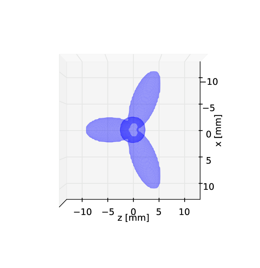
(a) Top

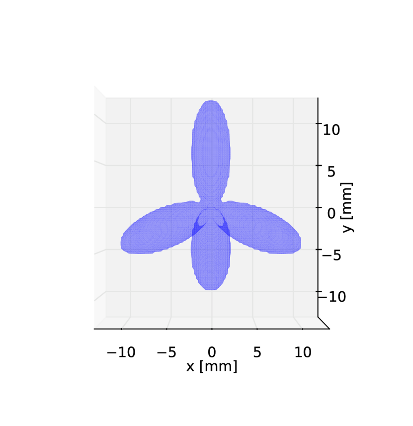
(b) Axial

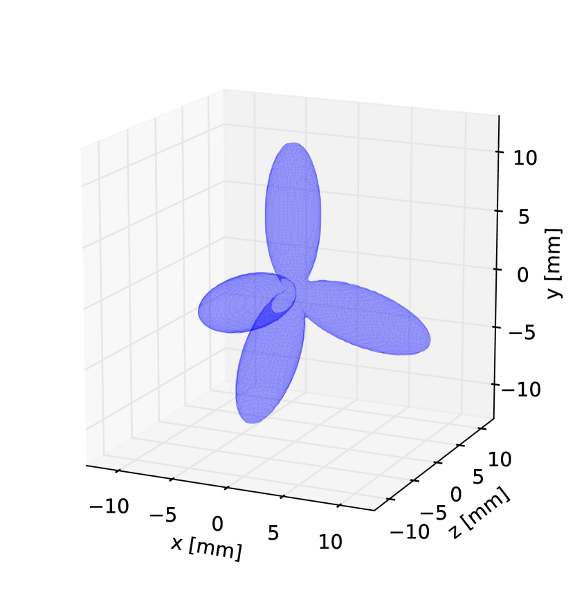
(c) Perspective

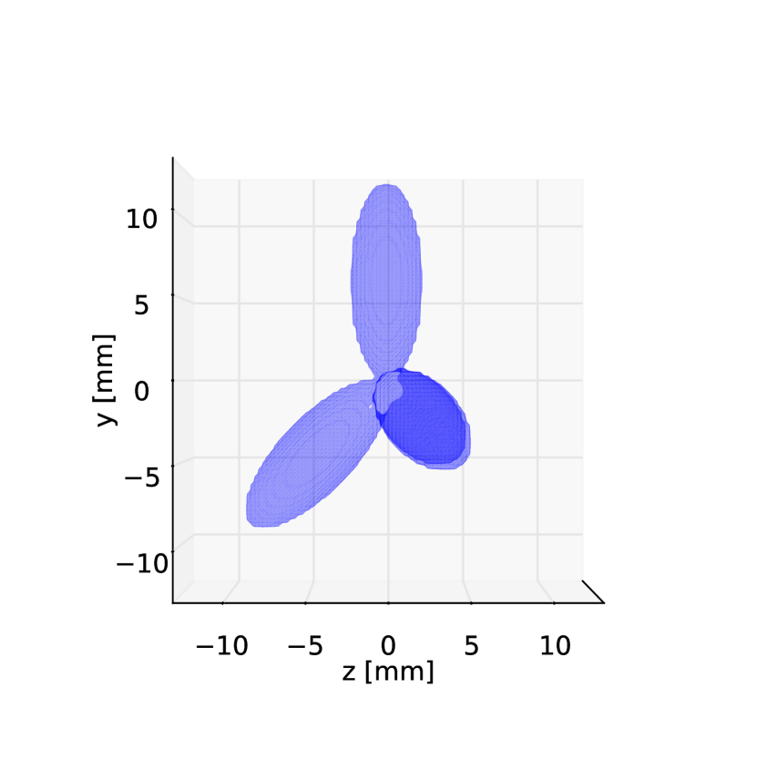
(d) Side

Figure 4: The four-pronged phantom used in the simulations.

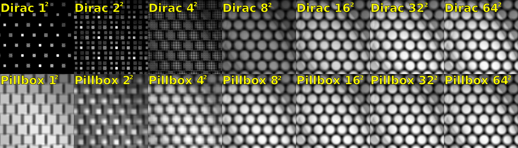
Figure 5: $256\times 256$-pixel subimages from the simulated plenoptic camera with different angular discretizations. As the angular discretization increases, both models produce high quality images, but the pillbox basis function is more accurate at coarser discretizations.

Figure 4 shows the four-pronged phantom we imaged in this experiment, and Figure 5 shows $256\times 256$ subimages from the simulated plenoptic camera at each parameterization of the angular plane we tested. Each number in the parameterization gives the coarseness of the discretization along the $s$ and $t$ directions; e.g., “Pillbox $8^{2}$” means a $8\times 8$ discretization of the angular plane using the pillbox angular basis function.

Both the Dirac and pillbox models produce high quality images at higher angular discretizations, but the Dirac model yields significant aliasing artifacts at lower discretizations. This is a well-known weakness of “pinhole camera” modeling from image-based rendering methods [39, 40], and is mitigated by using the pillbox basis function.

Figure 6(b) plots the normalized difference,

$$\text{NSD}{\left({\bm{y}}\right)} =\frac{{\left|\left|{\bm{y}}-{\bm{y}}_{\text{high-quality}}\right|\right|}^{2}}{{\left|\left|{\bm{y}}_{\text{high-quality}}\right|\right|}^{2}}$$

of each configuration to the highest-quality pinhole rendering, and confirms the superior accuracy of the pillbox angular plane discretization over the pinhole discretization. Since the higher quality rendering of the pillbox comes at essentially no additional computational time over the Dirac approach, as Figure 6(a) shows, we use the pillbox-based model for the following reconstructions.

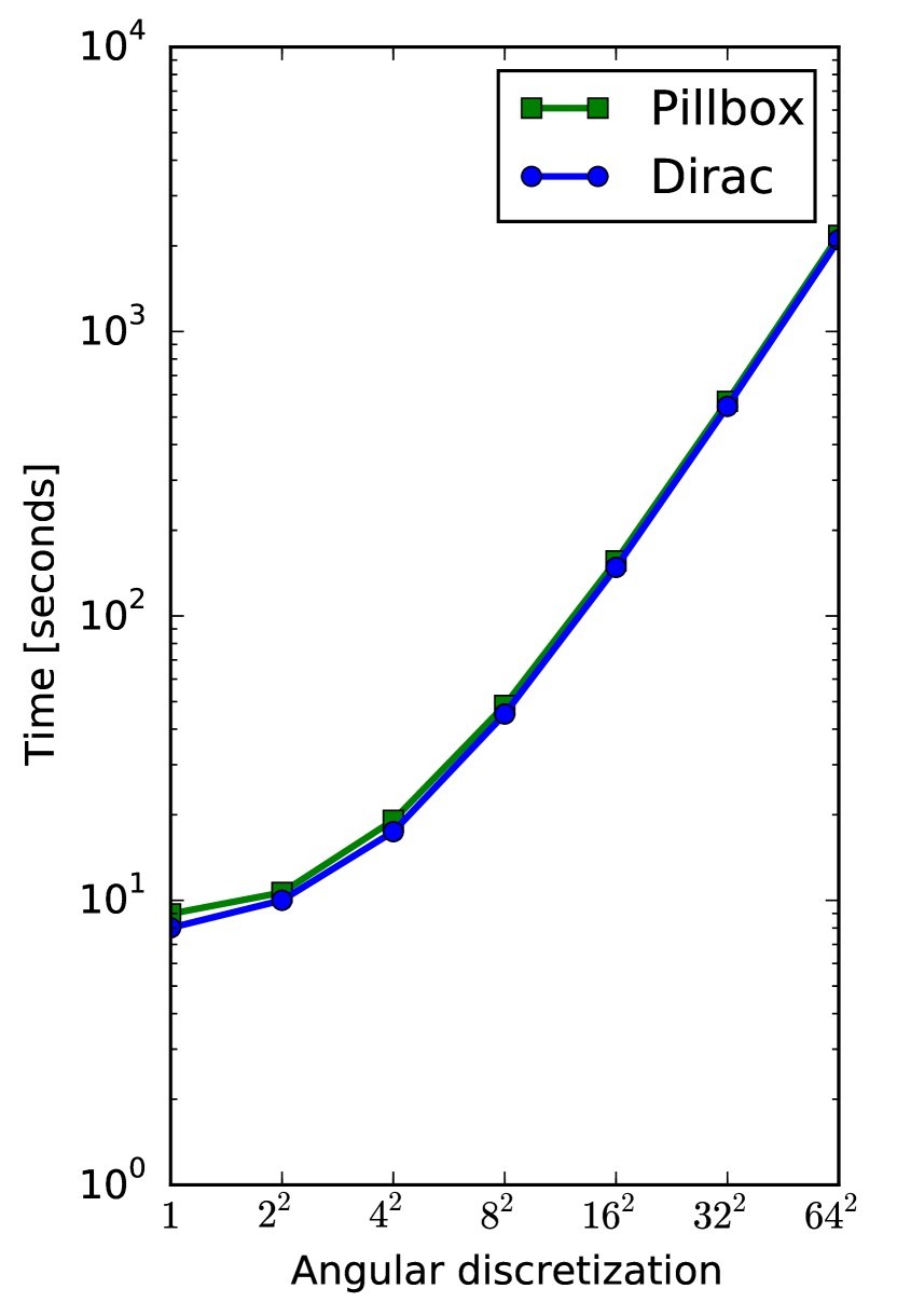
(a) Projection time

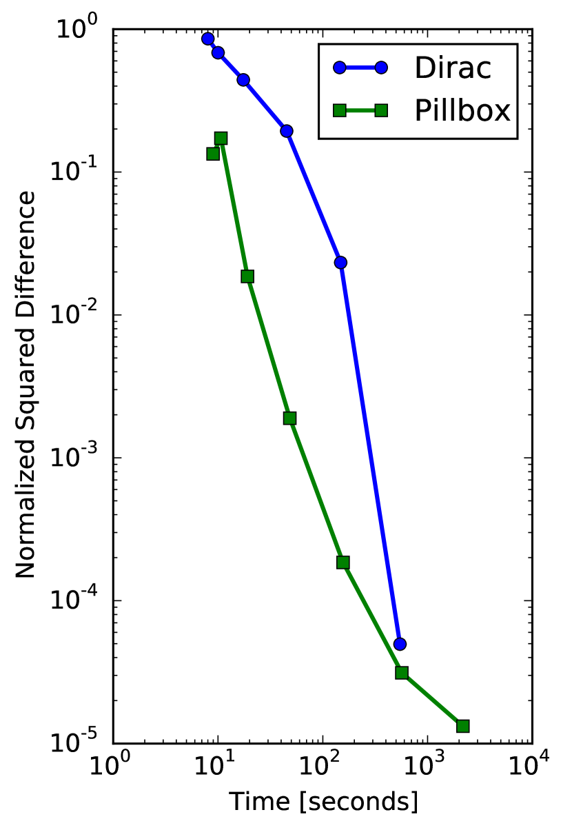
(b) Projection accuracy

Figure 6: Projection times and NSD for a the simulated plenoptic camera model. NSD is computed relative to the image from the Dirac image with $64\times 64$ angular discretization. The pillbox model is essentially as fast as the Dirac model, but produces more accurate results, particularly at coarser discretizations.

VI-B Single camera reconstruction

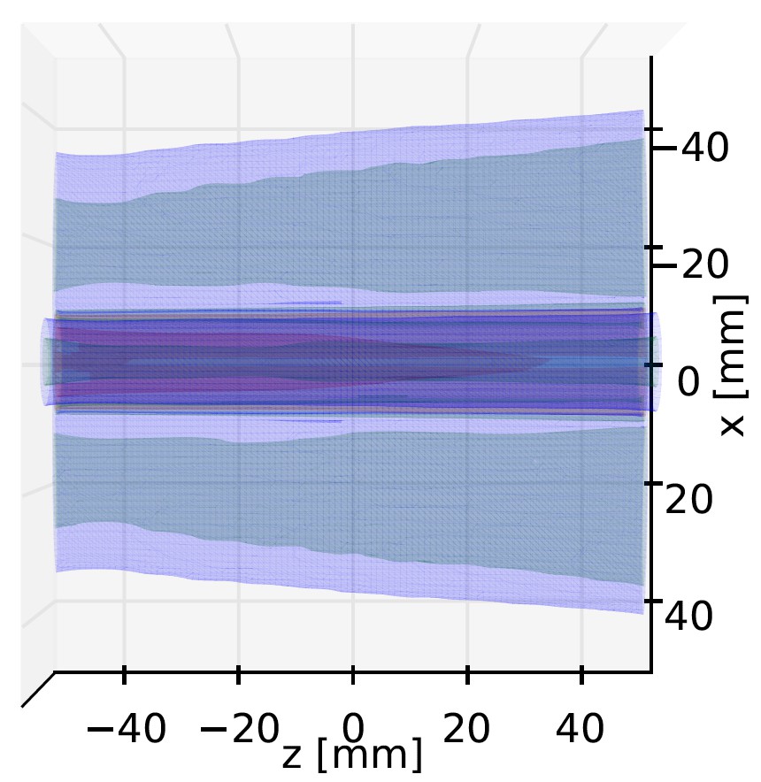
(a) Top

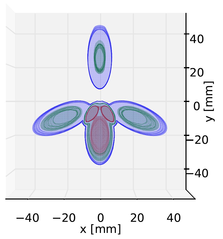
(b) Axial

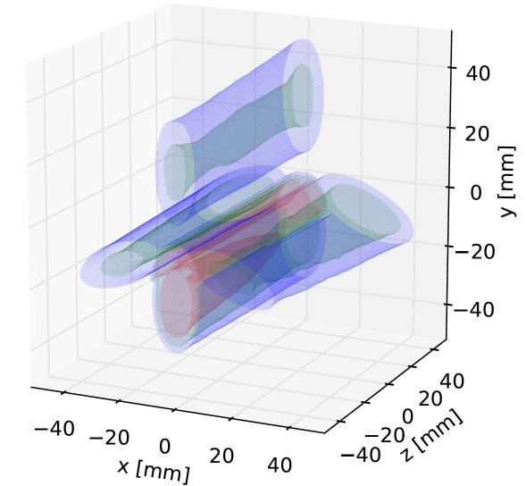
(c) Perspective

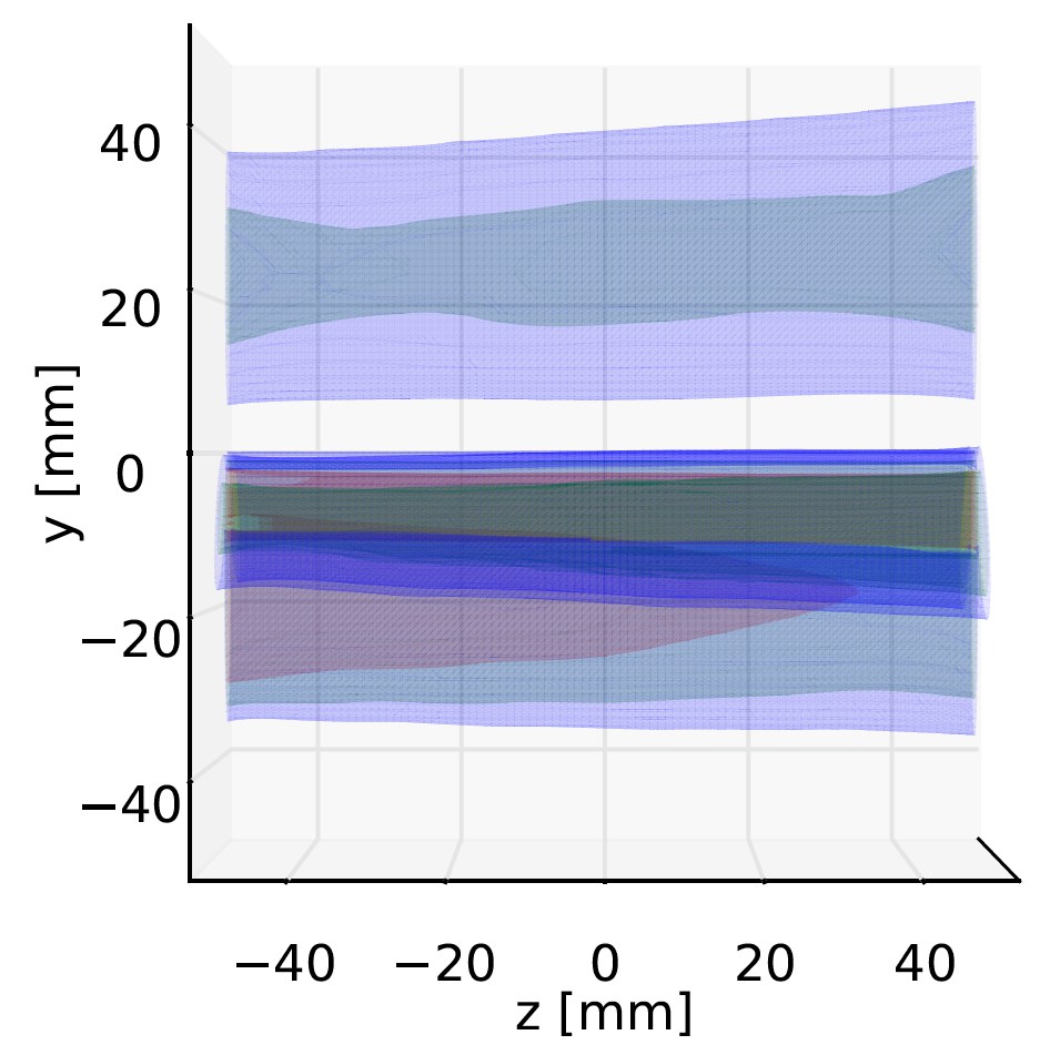
(d) Side

Figure 7: Simulated reconstruction from one plenoptic camera. The figures show level sets at 45% (blue), 60% (green) and 75% (red) of the reconstruction’s maximum value. The reconstruction has very poor axial ($z$) resolution.

We simulated image an of the four-pronged phantom taken by the plenoptic 2.0 camera in Table VI, shown in Figure 9(b), using the pinhole basis function and a $64\times 64$ angular plane discretization. We then reconstructed the image using a $16\times 16$ angular discretization using the pillbox basis function and $N_{\text{subset}}=2$ subset acceleration. The image is reconstructed onto a $100\times 100\times 100$ volume with $1~{}\text{mm}^{3}$ voxels; the data were generated from a $200\times 200\times 200$ volume with $\frac{1}{8}\text{mm}^{3}$ voxels to avoid an “inverse crime.” Each image update (subset) took about 70 seconds, and we ran the algorithm for 160 iterations.

Figure 7 shows level sets from the reconstructed image. The reconstruction has good transaxial ($xy$) resolution, but very poor axial ($z$) resolution. The reconstruction quality is too poor to be useful; this confirms earlier findings [41] using another system model [30] and similar reconstruction approach. We posit that the poor reconstruction quality is due to very limited angular information; the next section adds two regular cameras at $\pm 30^{\circ}$ to augment the missing angular information.

VI-C Three camera reconstruction

(a) Top

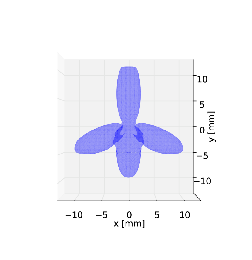
(b) Axial

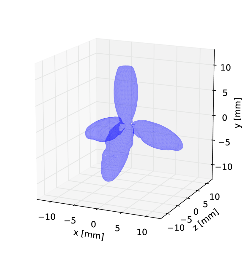
(c) Perspective

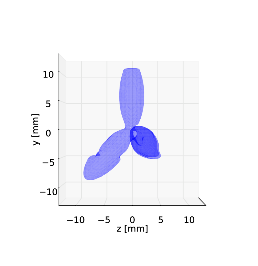
(d) Side

Figure 8: Simulated reconstruction from one plenoptic camera and two cameras. The figures show level sets at 40% of the reconstruction’s maximum value. The additional angular information from the two secondary cameras results in a high quality reconstruction.

TABLE VII: Simulated single-lens camera configuration

Property	Value
Lens focal length	30 mm
Lens radius	5 mm
Distance between lens and detector, $D$	31.3 mm
Detector pixel pitch	5 $\mu$m
Detector dimensions	$1024\times 1024$ pixels

We rendered images of the phantom from $\pm 30^{\circ}$ using the single lens camera described in Table VII. Figure 9 shows the three images used to perform the reconstruction. With the additional axial information, we found that a coarser angular discretization was acceptable for reconstruction: we used a $8\times 8$ pillbox discretization for each camera’s angular plane and no subset acceleration. Each iteration took about 49 seconds to run, and we ran 100 iterations of the proposed algorithm, but the iterates were stable after about 50 iterations.

Figure 8 shows the level sets of the reconstructed phantom. The additional angular information from the single lens cameras has a dramatic effect: the reconstructed images are much higher fidelity reconstructions of the original phantom in Figure 4. The proposed camera model also handles multiple cameras, gain estimation, and several camera types effectively. The next section, we validates the proposed technique using real data collected with a plenoptic camera and a rotational stage.

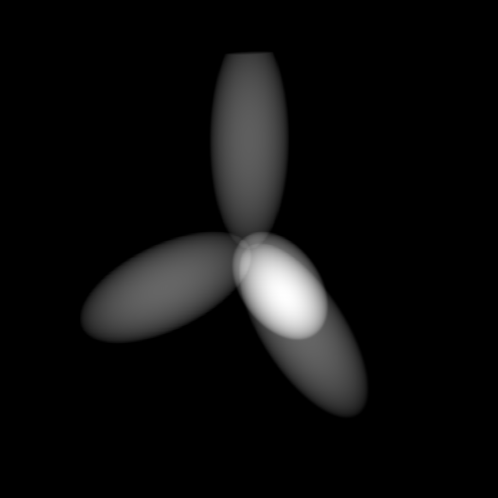
(a) $-30^{\circ}$ view

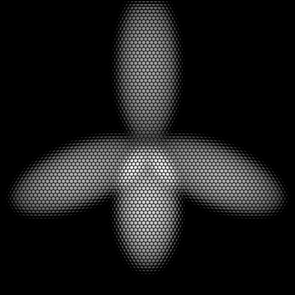
(b) Plenoptic image

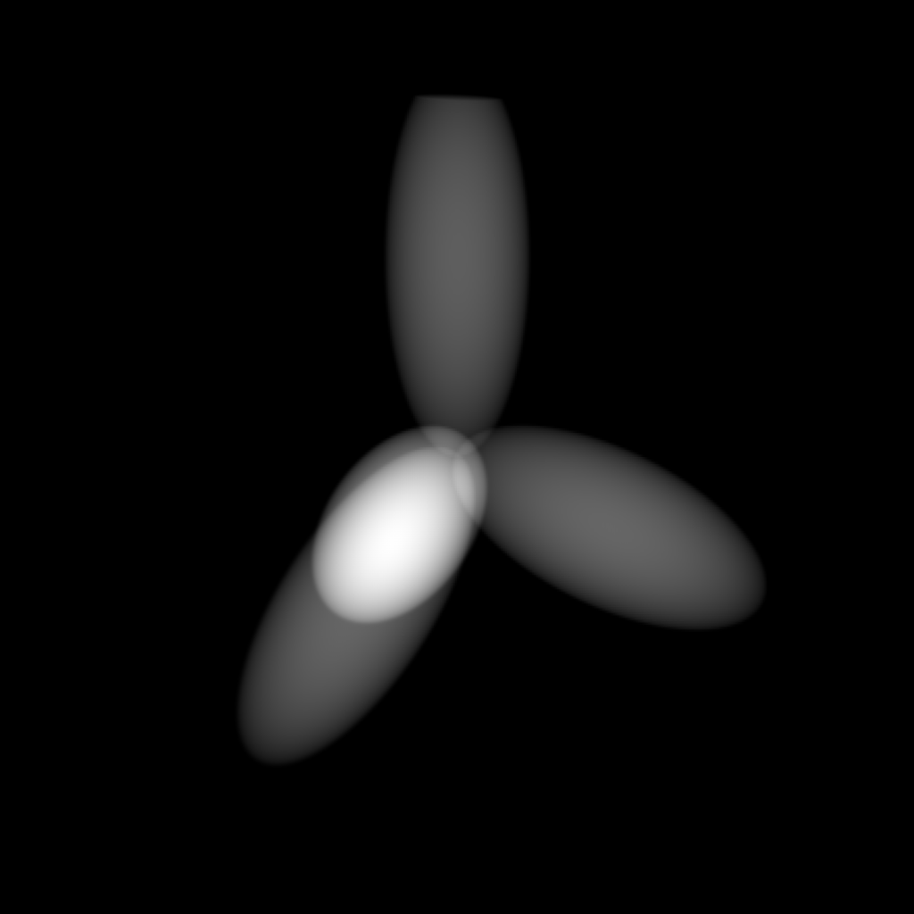
(c) $+30^{\circ}$ view

Figure 9: Three simulated views of a four-pronged torch phantom.

VI-D Flame reconstruction

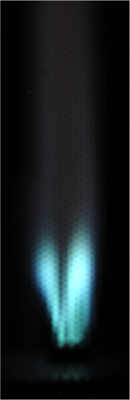
(a) $-15^{\circ}$

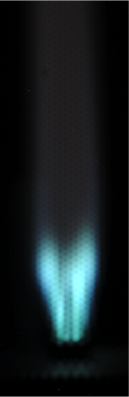
(b) Center

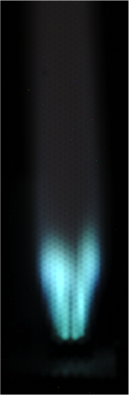
(c) $+15^{\circ}$

Figure 10: Subsets of refocused images created using Raytrix software for the flame reconstruction experiment. These images are for illustration; our reconstruction used the raw Bayer-encoded images from the camera.

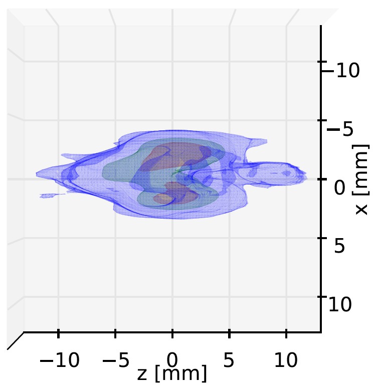
(a) Top

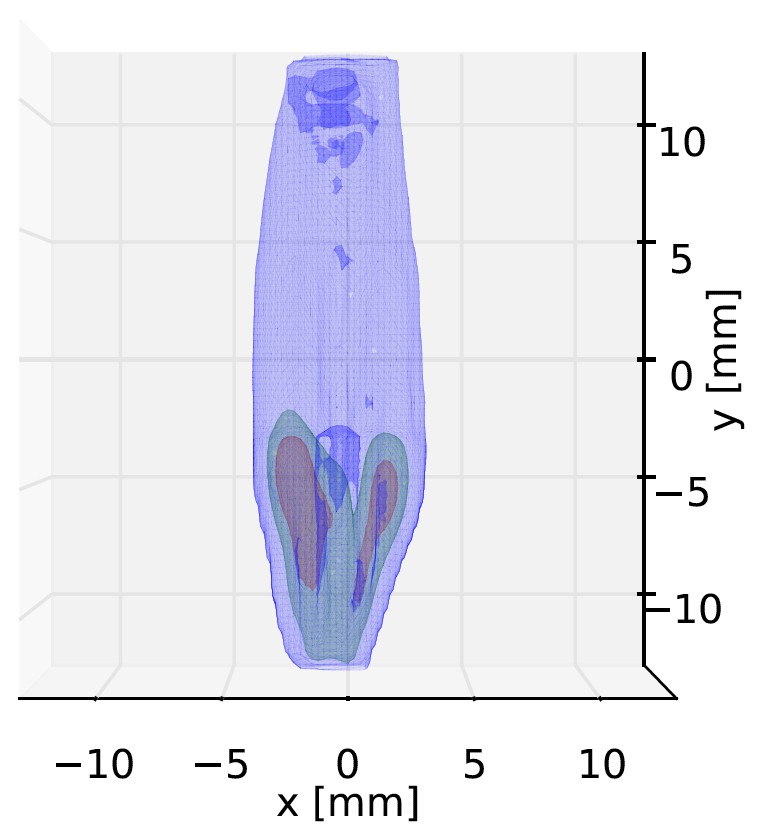
(b) Axial

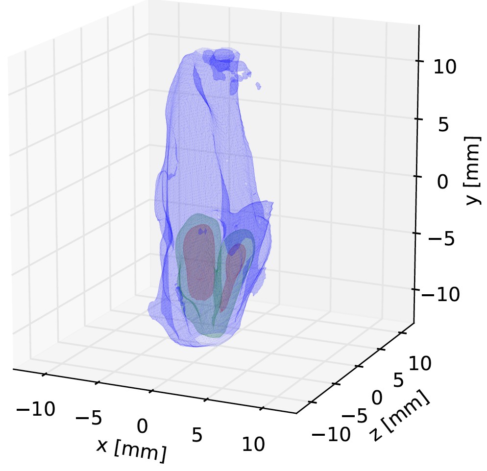
(c) Perspective

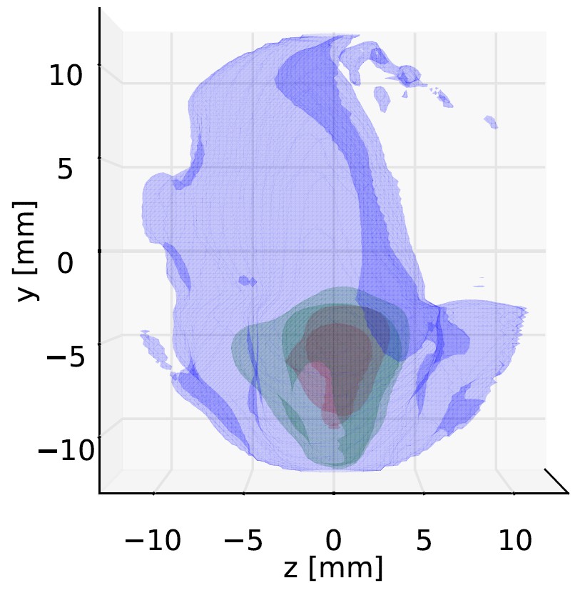
(d) Side

Figure 11: Reconstructed flame from three poses of the R29 camera. Isocontours shown at 2% (blue), 40% (green) and 70% (red) of the reconstruction’s maximum value.

We placed a burner on a rotating stage and took three images, each separated by $15^{\circ}$, with a Raytrix R29 camera attached to a 105 mm 1:2.8D macro lens; Figure 10 shows the center view. As Figure 10 shows, our detector has a region of damaged pixels. Although one could account for these defects in the reconstruction algorithm by identifying and down-weighting these pixels via the weights matrix $\bm{W}_{c}$, in this preliminary experiment we did not perform any such correction.

Some calibration had to be performed to fit our simple plenoptic approach (Figure 3) to the R29 camera. More sophisticated calibration techniques have been proposed by Raytrix [42] and others, but we use only a very simple method in this work. We performed a simple corner-based calibration to determine $D_{\mu m}$, the main lens-microlens array distance, and used vendor-given values for the main lens focal length, detector-microlens array distance $D_{\mu d}$, and microlens focal lengths. We tuned the aperture of the main lens to produce a simulated checkerboard image qualitatively similar to the calibration checkerboard image. The calibrated parameters themselves are proprietary, but the calibration code we used will be available under an open source license.

We reconstructed the flame onto a $100^{3}$ voxel grid with ${\left(\frac{1}{4}\right)}^{3}$ mm³. The weighting matrix $\bm{W}_{c}$ was used to extract only the green Bayer channel from the raw data. We used a $5\times 5$ angular discretization with $N_{\text{subset}}=4$ subsets; each iteration took about 50 seconds and we ran 100 iterations to produce the images in Figure 11.

Figure 11 shows that the proposed algorithm can successfully recover the 3D structure of the flame. There is some stretching in the axial direction that is particularly noticeable in the lower-valued and cooler (blue) flame. More sophisticated calibration and simultaneous capture of multiple perspectives (instead of the “rotate-and-shoot” acquisition used here), may mitigate these problems.

VII Conclusions and future work

We proposed an efficient light transport-based system model for camera inverse problems. The technique models cameras as compositions of light transport steps that can be efficiently implemented on modern computing hardware. In simulated experiments, we modeled a plenoptic 2.0 camera and a traditional single-lens camera and performed 3D flame reconstructions using a FISTA-based [34] algorithm. We also validated the proposed algorithm on 3D reconstruction problem with real data taken from a Raytrix R29 camera.

A drawback of many existing camera models for inverse problems is their reliance on precomputation and sparse linear algebra routines. These techniques are mathematically correct but often too inefficient to produce reconstructions quickly. The proposed model is efficient and flexible: the general-purpose reconstruction algorithm in this paper can perform a 3D reconstruction from three plenoptic camera images in under an hour on a single GPU, and more specialized algorithms would likely produce faster reconstructions. Furthermore, faster algorithms make dynamic time-varying 3D reconstructions more feasible.

Future work on handling nonideal optics will hopefully improve the reconstruction results reported in Section V. We also plan to apply the tools in this paper to other lightfield imaging and recovery tasks, along with more systematic quantitative results and comparisons of camera configurations for specific applications.

Appendix A Reconstruction cost function Hessian

This appendix shows that the Hessian of the reconstruction cost function (26) in terms of ${\bm{x}}$ (after minimization over the gains) is positive semidefinite and easily majorized.

For simplicity, first perform a change of variables to “absorb” the weights $\bm{W}_{c}$ to the system matrix ${\bm{A}}_{c}$ and the data ${\bm{y}}_{c}$. Perform the inner minimization over the camera gains ${\left\{\gamma_{c}\right\}}$:

$$\gamma_{c} =\frac{{\bm{y}}_{c}^{\intercal}{\bm{A}}_{c}{\bm{x}}}{{\bm{y}}_{c}^{\intercal}{\bm{y}}_{c}}.$$ (30)

Plug (30) into (26):

$$\mathop{\text{min}}_{{\left\{\gamma_{c}\right\}}}\Psi{\left({\bm{x}},{\left\{\gamma_{c}\right\}}\right)} =\frac{1}{2}{\left|\left|{\bm{A}}_{1}{\bm{x}}-{\bm{y}}_{1}\right|\right|}_{2}^{2}+\mathsf{R}{\left({\bm{x}}\right)}$$

$$+\sum_{c=2}^{N_{c}}\frac{1}{2}{\left|\left|{\left(\bm{I}-\frac{1}{{\left|\left|{\bm{y}}_{c}\right|\right|}^{2}}{\bm{y}}_{c}{\bm{y}}_{c}^{\intercal}\right)}{\bm{A}}_{c}{\bm{x}}\right|\right|}_{2}^{2}.$$ (31)

The Hessian of this resulting cost function is

$$\nabla^{2}_{\bm{x}}\mathop{\text{min}}_{{\left\{\gamma_{c}\right\}}}\Psi{\left({\bm{x}},{\left\{\gamma_{c}\right\}}\right)} ={\bm{A}}_{1}^{\intercal}{\bm{A}}_{1}+\nabla^{2}\mathsf{R}{\left({\bm{x}}\right)}+\sum_{c=2}^{N_{c}}{\bm{A}}_{c}^{\intercal}\bm{G}_{c}^{2}{\bm{A}}_{c}$$

$$\succeq{\bm{0}},$$ (32)

where $\bm{G}_{c}=\bm{I}-\frac{1}{{\left|\left|{\bm{y}}_{c}\right|\right|}^{2}}{\bm{y}}{\bm{y}}^{\intercal}$ is positive semidefinite but has spectral radius less than unity. Consequently,

$$\nabla^{2}_{\bm{x}}\mathop{\text{min}}_{{\left\{\gamma_{c}\right\}}}\Psi{\left({\bm{x}},{\left\{\gamma_{c}\right\}}\right)} \preceq\sum_{c=1}^{N_{c}}{\bm{A}}_{c}^{\intercal}{\bm{A}}_{c}+\nabla^{2}\mathsf{R}{\left({\bm{x}}\right)}$$

$$\preceq\bm{D}+\nabla^{2}\mathsf{R}{\left({\bm{x}}\right)}$$

$$\preceq\bm{D}+26\beta\bm{I},$$ (33)

where $\bm{D}$ is the usual diagonal majorizer for the data-fit terms [36]:

$$\bm{D} =\mathop{\text{diag}}_{j}{\left\{{\left[\sum_{c=1}^{N_{c}}{\bm{A}}_{c}^{\intercal}{\bm{A}}_{c}{\bm{1}}\right]}_{j}\right\}}.$$ (34)

References

- [1] D. G. Dansereau, O. Pizarro, and S. B. Williams, “Decoding, calibration and rectification for lenselet-based plenoptic cameras,” in Proc. IEEE Conf. on Comp. Vision and Pattern Recognition, 2013, pp. 1027–34.
- [2] O. Klehm, I. Ihrke, H.-P. Seidel, and E. Eisemann, “Volume stylizer: tomography-based volume painting,” in SIGGRAPH, 2013, pp. 161–8.
- [3] V. Todoroff, G. L. Besnerais, D. Donjat, F. Micheli, A. Plyer, and F. Champagnat, “Reconstruction of instantaneous 3D flow density fields by a new direct regularized 3DBOS method,” in 17th Intl. Symp. on Appl. of Laser Tech. to Fluid. Mech., 2014.
- [4] G. Wetzstein, I. Ihrke, and W. Heidrich, “Sensor saturation in Fourier multiplexed imaging,” in Proc. IEEE Conf. on Comp. Vision and Pattern Recognition, 2010, pp. 545–52.
- [5] I. Ihrke and M. Magnor, “Image-based tomographic reconstruction of flames,” in Proc. SIGGRAPH/Eurographics Symp. on Comp. Anim., 2004, pp. 365–73.
- [6] A. Schwarz, “Multi-tomographic flame analysis with a schlieren apparatus,” Meas. Sci. and Tech., vol. 7, pp. 406–13, Mar. 1996.
- [7] X. Li and L. Ma, “Volumetric imaging of turbulent reactive flows at kHz based on computed tomography,” Optics Express, vol. 22, no. 4, pp. 4768–78, Feb. 2014.
- [8] S. W. Hasinoff and K. N. Kutulakos, “Photo-consistent 3D fire by flame-sheet decomposition,” in Proc. Intl. Conf. Comp. Vision, vol. 2, 2003, pp. 1184–91.
- [9] R. Ng, M. Levoy, M. Brédif, G. Duval, M. Horowitz, and P. Hanrahan, “Light field photography with a hand-held plenoptic camera,” 2005, stanford Tech Report CTSR 2005-02, micro-lens.
- [10] C. Perwass and L. Wietzke, “Single lens 3D-camera with extended depth-of-field,” in Proc. SPIE 8291 Human Vision and Electronic Imaging XVII, 2012, p. 829108.
- [11] K. Marwah, G. Wetzstein, Y. Bando, and R. Raskar, “Compressive light field photography using overcomplete dictionaries and optimized projections,” ACM Trans. on Graphics, vol. 32, no. 4, pp. 46:1–12, Jul. 2013.
- [12] G. E. Elsinga, F. Scarano, B. Wieneke, and B. W. Van Oudheusden, “Tomographic particle image velocimetry,” Experiments in Fluids, vol. 41, no. 6, pp. 933–47, Dec. 2006.
- [13] T. W. Fahringer and B. S. Thurow, “Tomographic reconstruction of a 3-D flow field using a plenoptic camera,” in AIAA Fluid Dynamics Conf., 2012, p. 2826.
- [14] M. L. Greene and V. Sick, “Volume-resolved flame chemiluminescence and laser-induced fluorescence imaging,” Appl Phys B, vol. 113, no. 1, pp. 87–92, Oct. 2013.
- [15] S. A. Shroff and K. Berkner, “Image formation analysis and high resolution image reconstruction for plenoptic imaging systems,” Appl. Optics, vol. 52, no. 10, pp. D22–31, Apr. 2013.
- [16] W. Cai, X. Li, and L. Ma, “Practical aspects of implementing three-dimensional tomography inversion for volumetric flame imaging,” Appl. Optics, vol. 52, no. 33, pp. 8106–16, Nov. 2013.
- [17] C.-K. Liang, Y.-C. Shih, and H. H. Chen, “Light field analysis for modeling image formation,” IEEE Trans. Im. Proc., vol. 20, no. 2, pp. 446–60, Feb. 2011.
- [18] C.-K. Liang and R. Ramamoorthi, “A light transport framework for lenslet light field cameras,” ACM Trans. on Graphics, vol. 34, no. 2, pp. 16:1–16:19, Mar. 2015.
- [19] B. M. W. Tsui, H.-B. Hu, D. R. Gilland, and G. T. Gullberg, “Implementation of simultaneous attenuation and detector response correction in SPECT,” IEEE Trans. Nuc. Sci., vol. 35, no. 1, pp. 778–83, Feb. 1988.
- [20] R. M. Leahy and J. Qi, “Statistical approaches in quantitative positron emission tomography,” Statistics and Computing, vol. 10, no. 2, pp. 147–65, Apr. 2000.
- [21] M. Broxton, L. Grosenick, S. Yang, N. Cohen, A. Andalman, K. Deisseroth, and M. Levoy, “Wave optics theory and 3-D deconvolution for the light field microscope,” Optics Express, vol. 21, no. 21, pp. 25 418–39, Oct. 2013.
- [22] M. Levoy and P. Hanrahan, “Light field rendering,” in SIGGRAPH, 1996, pp. 31–42.
- [23] Y. Censor, “Finite series expansion reconstruction methods,” Proc. IEEE, vol. 71, no. 3, pp. 409–19, Mar. 1983.
- [24] R. M. Lewitt and S. Matej, “Overview of methods for image reconstruction from projections in emission computed tomography,” Proc. IEEE, vol. 91, no. 10, pp. 1588–611, Oct. 2003.
- [25] H. Nien, “Model-based X-ray CT image and light field reconstruction using variable splitting methods,” Ph.D. dissertation, Univ. of Michigan, Ann Arbor, MI, 48109-2122, Ann Arbor, MI, 2014. [Online]. Available: https://hdl.handle.net/2027.42/108981
- [26] S. D. Babacan, R. Ansorge, M. Luessi, P. R. Mataran, R. Molina, and A. K. Katsaggelos, “Compressive light field sensing,” IEEE Trans. Im. Proc., vol. 21, no. 12, pp. 4746–57, Dec. 2012.
- [27] M. Unser, P. Thevenaz, and L. Yaroslavsky, “Convolution-based interpolation for fast, high quality rotation of images,” IEEE Trans. Im. Proc., vol. 4, no. 10, pp. 1371–81, Oct. 1995.
- [28] A. W. Paeth, “A fast algorithm for general raster rotation,” in Proc. Graphics Interface, 1986, pp. 77–81. [Online]. Available: http://doi.org/10.20380/GI1986.15
- [29] J. Schwiegerling, “Plenoptic camera image simulation for reconstruction algorithm verification,” in Proc. SPIE 9193 Novel Optical Systems Design and Optimization XVI, 2014, p. 91930V.
- [30] T. E. Bishop and P. Favaro, “The light field camera: extended depth of field, aliasing, and superresolution,” IEEE Trans. Patt. Anal. Mach. Int., vol. 34, no. 5, pp. 972–86, May 2012.
- [31] Y. Long, J. A. Fessler, and J. M. Balter, “3D forward and back-projection for X-ray CT using separable footprints,” IEEE Trans. Med. Imag., vol. 29, no. 11, pp. 1839–50, Nov. 2010.
- [32] D. L. Snyder, A. M. Hammoud, and R. L. White, “Image recovery from data acquired with a charge-coupled-device camera,” J. Opt. Soc. Am. A, vol. 10, no. 5, pp. 1014–23, May 1993.
- [33] D. L. Snyder, C. W. Helstrom, A. D. Lanterman, M. Faisal, and R. L. White, “Compensation for readout noise in CCD images,” J. Opt. Soc. Am. A, vol. 12, no. 2, pp. 272–83, Feb. 1995.
- [34] A. Beck and M. Teboulle, “A fast iterative shrinkage-thresholding algorithm for linear inverse problems,” SIAM J. Imaging Sci., vol. 2, no. 1, pp. 183–202, 2009.
- [35] D. Kim, S. Ramani, and J. A. Fessler, “Combining ordered subsets and momentum for accelerated X-ray CT image reconstruction,” IEEE Trans. Med. Imag., vol. 34, no. 1, pp. 167–78, Jan. 2015.
- [36] H. Erdogan and J. A. Fessler, “Ordered subsets algorithms for transmission tomography,” Phys. Med. Biol., vol. 44, no. 11, pp. 2835–51, Nov. 1999.
- [37] H. Guan and R. Gordon, “A projection access order for speedy convergence of ART (algebraic reconstruction technique): a multilevel scheme for computed tomography,” Phys. Med. Biol., vol. 39, no. 11, pp. 2005–22, Nov. 1994.
- [38] S. Ramani, Z. Liu, J. Rosen, J.-F. Nielsen, and J. A. Fessler, “Regularization parameter selection for nonlinear iterative image restoration and MRI reconstruction using GCV and SURE-based methods,” IEEE Trans. Im. Proc., vol. 21, no. 8, pp. 3659–72, Aug. 2012.
- [39] Z. Lin and H.-Y. Shum, “On the number of samples needed in light field rendering with constant-depth assumption,” in Proc. IEEE Conf. on Comp. Vision and Pattern Recognition, 2000.
- [40] J. Chai, X. Tong, S. Chan, and H. Shum, “Plenoptic sampling,” in SIGGRAPH, 2000, pp. 307–18.
- [41] H. Nien, V. Sick, and J. A. Fessler, “Model-based image reconstruction of chemiluminescence using plenoptic 2.0 camera,” in Proc. IEEE Intl. Conf. on Image Processing, 2015, pp. 359–63.
- [42] O. Johannsen, C. Heinze, B. Goldluecke, and C. Perwass, “On the calibration of focused plenoptic cameras,” in Time-of-Flight and Depth Imaging. Sensors, Algorithms, and Applications: Dagstuhl 2012 Seminar on Time-of-Flight Imaging and GCPR 2013 Workshop on Imaging New Modalities, M. Grzegorzek, C. Theobalt, R. Koch, and A. Kolb, Eds. Berlin: Springer, 2013, pp. 302–17.