Measurement of the $\ce{{}^{\textbf{8}}}$B Solar Neutrino Flux in SNO+ with Very Low Backgrounds

Abstract

A measurement of the $\ce{{}^{8}B}$ solar neutrino flux has been made using a 69.2 kt-day dataset acquired with the SNO+ detector during its water commissioning phase. At energies above 6 MeV the dataset is an extremely pure sample of solar neutrino elastic scattering events, owing primarily to the detector’s deep location, allowing an accurate measurement with relatively little exposure. In that energy region the best fit background rate is $0.25^{+0.09}_{-0.07}$ events/kt-day, significantly lower than the measured solar neutrino event rate in that energy range, which is $1.03^{+0.13}_{-0.12}$ events/kt-day. Also using data below this threshold, down to 5 MeV, fits of the solar neutrino event direction yielded an observed flux of $2.53^{+0.31}_{-0.28}$(stat.)${}^{+0.13}_{-0.10}$(syst.)$\times 10^{6}$ cm^-2s^-1, assuming no neutrino oscillations. This rate is consistent with matter enhanced neutrino oscillations and measurements from other experiments.

I Introduction

Neutrinos are produced in the core of the Sun through a variety of nuclear reactions. The $\ce{{}^{8}B}$ $\beta^{+}$ decay (Q$\leavevmode\nobreak\ \approx\leavevmode\nobreak\$18 MeV), dominates the high-energy portion of the solar neutrino spectrum Bahcall et al. (2005). Pioneering measurements of the solar neutrino fluxes, including $\ce{{}^{8}B}$, were made by the chlorine and gallium radiochemical experiments Cleveland et al. (1998); Abdurashitov et al. (2003); Altmann et al. (2005); Hampel et al. (1999), and the first real-time measurement of solar neutrinos was made by the Kamiokande-II experiment Hirata et al. (1990). The measurement of $\ce{{}^{8}B}$ solar neutrinos by the Sudbury Neutrino Observatory (SNO), along with measurements of atmospheric and solar neutrinos from Super Kamiokande (Super-K), led to the resolution of the solar neutrino problem and the initial determination of solar neutrino mixing parameters Bahcall and Ulrich (1988); Ahmad et al. (2001, 2002); Fukuda et al. (1998, 2001). After the first measurements from SNO and Super-K, further $\ce{{}^{8}B}$ solar neutrino measurements have been made by the liquid scintillator detectors Borexino Bellini et al. (2010) and KamLAND Abe et al. (2011). These two experiments have also measured solar neutrinos from reactions other than $\ce{{}^{8}B}$  Agostini et al. (2018); Bellini et al. (2014); Gando et al. (2015).

Due to the depth and flat overburden at SNOLAB, SNO+ has an extremely low rate of cosmic-ray muons: roughly three per hour. At this rate it is practical to veto all events for a period of time after each muon (see Sec. VI) to reduce spallation backgrounds. As a result, the rate of backgrounds due to cosmogenic activation and spallation is extremely low.

This article presents the first solar neutrino results from the SNO+ experiment. The low level of backgrounds permits a measurement of the $\ce{{}^{8}B}$ solar neutrino flux down to 5 MeV with the first 8 months of data. The analysis exercises many tools distinct from those used by the SNO Collaboration, including new precision modeling of the detector, energy and vertex reconstruction, instrumental background rejection, and a well understood level of intrinsic radioactive contamination in all detector components. These will be critical to the future sensitivity of SNO+ in searches for neutrinoless double beta decay and measurements of low-energy solar neutrinos Andringa et al. (2016).

Elastic scattering of electrons by neutrinos, $\nu_{x}$ $+$ $e^{-}$ $\rightarrow$ $\nu_{x}$ $+$ $e^{-}$ ($x$ = $e$, $\mu$, $\tau$), can occur through either a neutral current interaction for neutrinos of all flavors, or a charged current interaction, for electron neutrinos only. The scattered electron’s direction is correlated with the direction of the incident neutrino, so recoil electrons from solar neutrino interactions will typically produce Cherenkov radiation that is directed away from the Sun. The analysis presented here exploits this correlation to measure the solar neutrino flux and spectrum.

II Detector

The SNO+ detector inherits much of its infrastructure from the SNO experiment Boger et al. (2000). The detector is located at a depth of approximately 6000 m water equivalent below surface; it consists of a spherical 6 m radius acrylic vessel (AV) suspended within a urylon-lined, barrel-shaped cavity that is 11 m in radius and 34 m tall; the cavity is filled with purified water. For the data in this analysis the AV was filled with 0.9 kt of “light” water ($\ce{H_{2}O}$), as opposed to the heavy water ($\ce{D_{2}O}$) used in SNO. Surrounding the AV are 9394 inward-looking 8-inch photomultiplier tubes (PMTs) housed within a geodesic stainless steel PMT support structure of average radius 8.4 m. Mounted on the outside of the support structure are 90 outward looking (OWL) PMTs that serve as a muon veto. Each of the SNO+ PMTs is surrounded by a reflective concentrator to increase its effective light collection. A number of the original SNO PMTs were removed to accommodate a hold-down rope net that will counteract the buoyant forces on the AV when it is filled with liquid scintillator Bialek et al. (2016).

The PMTs are read out by custom data acquisition (DAQ) electronics that have been largely carried over from SNO; parts of the trigger and readout system have been upgraded, allowing a lower trigger threshold. A separate paper discussing in greater detail the SNO+ detector is forthcoming.

III Simulation

A Geant4-based Agostinelli et al. (2003) Monte Carlo (MC) simulation framework of the SNO+ detector (“RAT”) was used to determine the expected detector response and selection efficiency for solar neutrino interactions. The $\ce{{}^{8}B}$ neutrino spectrum from Winter et al. Winter et al. (2006), and a model of the differential and total cross-sections for electron-neutrino scattering from Bahcall et al. Bahcall et al. (1995), were used to calculate the expected interaction rate. The detector simulation models all relevant effects after the initial particle interaction, including Cherenkov light production, electron scattering processes, photon propagation and detection, and the DAQ electronics. The geometries and material properties in the simulation were determined using ex-situ measurements and in-situ calibrations. The input parameters for the DAQ simulation were matched to the detector settings and channel status on a run-by-run basis.

IV Reconstruction

For each detected or simulated event, the position, time, direction, and energy were reconstructed under the assumption that all light produced is Cherenkov radiation from an electron. The direction, time, and position were determined simultaneously through a likelihood fit based on the pattern and timing of the PMT signals in the event. The likelihood was determined using expected distributions of photon timing and angular spread, which are calculated using MC simulation. Only signals originating from well-calibrated channels were used in the fit.

Energy was determined separately using the position, time, direction, and the number of PMT signals in a prompt 18 ns window as inputs; the prompt time window mitigates the effect of PMT noise and of light that follows a difficult to model path between creation and detection. Using the inputs, the reconstruction algorithm then uses a combination of MC simulation and analytic calculation to estimate the event energy that is most likely to produce the observed number of PMT signals. The same reconstruction algorithms were used for both simulated and detected events.

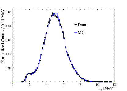
(a)

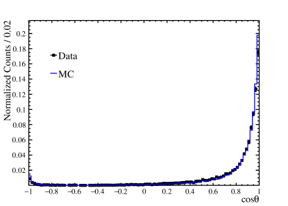
(b)

FIG. 1: Energy (a) and direction (b) reconstruction comparison between Monte Carlo simulation and data for $\ce{{}^{16}N}$ events. Here $T_{e}$ is the electron kinetic energy, and $\theta$ is the angle between the reconstructed direction of an event and the direction vector pointing from the source position to the event’s reconstructed position.

V Calibration

Calibration data were taken with a deployed $\ce{{}^{16}N}$ source Dragowsky et al. (2002), which primarily produces a tagged 6.1 MeV $\gamma$-ray. These data are used for calibrating detector components and evaluating systematic uncertainties of reconstructed quantities.

The source position was controlled using a system of ropes to perform a 3-dimensional scan of the space inside the AV, and a 1-dimensional vertical scan in the region between the AV and the PMTs. For the purpose of evaluating systematics, the distributions of events in position, direction, and energy were fitted with response functions. The parameters from fits performed on data and MC simulation were compared to assign systematic uncertainties on each reconstructed quantity. Figure 1 shows comparisons between simulation and data for the reconstructed energy and direction of $\ce{{}^{16}N}$ events.

The 6.1 MeV $\ce{{}^{16}N}$ $\gamma$-ray typically Compton scatters in the detector to produce one or more electrons that reconstruct to energies peaking near 5 MeV. In addition to Compton scattering, energy deposition in the source container also produces a substantial tail at lower energies. This tail fades out below about 1.7 MeV due to the detector trigger thresholds (see Fig. 1a). The energy resolution is composed of several effects including Compton scattering, detector resolution, and photon statistics; the latter being dominant. In the fit of the energy response function, the detector resolution was modeled as Gaussian and convolved with an $\ce{{}^{16}N}$ energy spectrum determined from MC simulation to account for the other two components. The resulting fractional uncertainty on the resolution within the fiducial volume and at kinetic energy $T_{e}$ is $0.018\sqrt{T_{e}/\text{MeV}}$; the fractional energy scale uncertainty is $2.0\%$. Similarly, for the position fit, the response function includes a convolution with the angular distribution of photon production to account for the non-negligible mean free path of the $\ce{{}^{16}N}$ $\gamma$-ray. The photon production distribution was also determined from MC simulation. More information about the $\ce{{}^{16}N}$ source analysis is available in Ref. Anderson et al. (2018), in which other water phase physics results from SNO+ are presented.

VI Dataset

Data for this analysis were gathered from May through December, 2017. Calibrations and detector maintenance were also performed during this period. Data taking periods were split into runs; the typical run length was between 30 and 60 minutes. Each run was checked against a number of criteria to ensure its quality. This included checks on the spatial uniformity of PMT signals, trigger rate, laboratory activity, and detector stability.

Within each run, muons and interactions from atmospheric neutrinos were tagged using the number of OWL PMT signals in an event and the number of events that follow closely in time. After each muon or atmospheric event, a 20 second deadtime was introduced to reduce backgrounds from cosmogenically produced isotopes, such as $\ce{{}^{16}N}$. Additional adjustments to the overall livetime were made to account for removal of time-correlated instrumental backgrounds. The resulting dataset contains 120 days of data and a corresponding livetime of 114.7 days, or 69.2 kt-days exposure with the fiducial volume cut described in Sec. VII.

VII Analysis

For each event, a suite of low-level cuts were applied to reject events originating from instrumental effects, and to ensure that the events had energies high enough to lie in a region of well-understood and near-perfect trigger efficiency. The trigger efficiency cut requires the number of PMT signals in a 100 ns coincidence window to be above a certain threshold. During the first 60% of dataset livetime, the threshold for this cut was $23$, while the trigger threshold itself was $15$ in-time signals. For the remaining section of data, the trigger threshold was lowered to $7$ in-time PMT signals and the corresponding trigger efficiency cut was $10$.

For events passing the low level cuts, it was further required that the vertex reconstruction fits successfully converged. Unsuccessful fits can occur if an event takes place in an optically complicated region of the detector, e.g., near the cylindrical chimney at the top of the AV. These regions often distort the light distribution from an event such that its vertex cannot be reliably determined.

A fiducial volume cut was then introduced requiring that each event reconstruct within 5.3 m of the detector center, reducing backgrounds from events originating on or outside the AV. A more restrictive cut on position was used for the beginning of data taking to minimize the impact of an increased rate of external backgrounds in the upper half of the detector. For that data, events observed in the upper half of the detector were required to be within 4.2 m of the center. The more restrictive cut was applied for $13\%$ of the dataset livetime.

After vertex reconstruction, additional cuts were placed on the timing and isotropy of PMT signals in each event. These cuts removed residual contamination from instrumental backgrounds (which have neither the prompt timing nor angular distribution of Cherenkov light), as well as events with poorly fit vertices. The timing cut required at least 55% of the PMT signals occur within a time-of-flight corrected prompt time window of width 7.5 ns. Isotropy was parameterised by $\beta_{14}$, a value determined by the first and fourth Legendre polynomials of the angular distribution of PMT signals within an event Aharmim et al. (2010). Events were required to have $\beta_{14}$ is between $-0.12$ and $0.95$.

A final cut was placed on the reconstructed kinetic energy of each event, selecting only events within the energy region 5.0 to 15.0  MeV, removing most of the backgrounds from radioactivity and atmospheric neutrino interactions; the only solar neutrinos with a significant flux in this energy region are $\ce{{}^{8}B}$ neutrinos. The fiducial volume and energy cuts select $21.4\%$ of simulated solar $\nu_{e}$ events that interact within the AV; events were simulated according to the $\ce{{}^{8}B}$ energy spectrum. The efficiencies of the other cuts on events that are within the energy region and fiducial volume are given in Table 1. Table 2 shows the effect of each cut on the dataset.

Selection	Passing MC Fraction
Total (after energy & position cuts)	1.0
Low-level cuts	0.988
Trigger Efficiency	0.988
Hit Timing	0.988
Isotropy	0.986

Table 1: Efficiency for each cut on MC simulated solar $\nu_{e}$ events that are within the fiducial volume and the energy region.

Selection	Passing Triggers
Total	12 447 734 554
Low-level cuts	4 547 357 090
Trigger Efficiency	126 207 227
Fit Valid	31 491 305
Fiducial Volume	6 958 079
Hit Timing	2 752 332
Isotropy	2 496 747
Energy	820

Table 2: Dataset reduction for each applied cut. The second column is the number of triggered events from the detector that pass each cut.

Since the direction of the recoil electron in a solar neutrino scattering event is correlated with the position of the Sun, the rate of solar neutrino events in the dataset was extracted by fitting the distribution of events in $\cos\theta_{\text{sun}}$, where $\theta_{\text{{sun}}}$ is the angle between an event’s reconstructed direction and the vector pointing directly away from the Sun at the time of the event. The rate of radioactive backgrounds present in the dataset can be determined as one of the parameters in the fit, so no a priori knowledge of the background rate was required.

Events with reconstructed kinetic energy, $T_{e}$, between $5.0$ and $10.0$ MeV were distributed among five uniformly wide bins, and a single bin from $10.0$ to $15.0$ MeV. In each energy bin, a maximum likelihood fit was performed on the distribution of events in $\cos\theta_{\text{{sun}}}$ to determine the rate of solar neutrino events and the rate of background events as a function of energy. The expected distribution for solar neutrino events in $\cos\theta_{\text{{sun}}}$ was calculated from MC simulation. The PDF for background events was taken to be uniform in $\cos\theta_{\text{{sun}}}$. The best fit flux over all energies was found by maximizing the product of the likelihoods from the fit in each energy bin. The resulting likelihood function is given by

$$\mathcal{L}(S ,\mathbb{B},\delta_{\theta}|\mathbb{n},\mu_{\theta},\sigma_{\theta})=$$

$$\mathcal{N}(\delta_{\theta},\mu_{\theta},\sigma_{\theta})\prod_{j=0}^{N_{E}}\prod^{N_{\theta}}_{i=0}\text{Pois}\left(n_{ij},\,B_{j}+S\,p_{ij}(\delta_{\theta})\right)\text{.}$$ (1)

The number of energy bins and angular bins are represented by $N_{E}$ and $N_{\theta}$ respectively. $S$ is the solar neutrino interaction rate and is the parameter of interest for this analysis, $B_{j}$ is the background rate in each energy bin. $\mathcal{N}$ represents a normalized Gaussian distribution. The $\delta_{\theta}$ parameter represents an adjustment to the angular resolution; $\mu_{\theta}$ and $\sigma_{\theta}$ are respectively the best fit and the constraint on $\delta_{\theta}$ from the $\ce{{}^{16}N}$ source analysis. The number of observed counts in the $i^{th}$ angular bin and $j^{th}$ energy bin is given by $n_{ij}$, and $p_{ij}(\delta_{\theta})$ is the corresponding predicted solar probability density for a given angular resolution parameter. $\text{Pois}\left(k,\lambda\right)$ is the value of the Poisson distribution at the value $k$ for a rate parameter $\lambda$.

Systematic uncertainties were propagated by varying the reconstructed quantities for each simulated event. A fit was then performed with each modified solar PDF to determine the effect the systematic uncertainty has on the final result. Because this analysis relies heavily on direction reconstruction, the angular resolution ($\delta_{\theta}$) was treated as a nuisance parameter in the fit for the solar flux. Details about the systematic uncertainties can be found in Ref. Anderson et al. (2018).

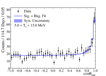
FIG. 2: Distribution of event direction with respect to solar direction. The systematic error bar includes angular correlated and uncorrelated errors.

VIII Results

Figure 2 shows the distribution of events in $\cos\theta_{\text{{sun}}}$ for events over the entire energy range of $5$ to $15$ MeV and the fit to that distribution. The fit gives a solar event rate of $1.30\pm 0.18$ events/kt-day and background rate of $10.23\pm 0.38$ events/kt-day. Performing a similar fit in each individual energy bin yielded a best fit solar flux as a function of energy. The fits were combined, in accordance with Eq. 1, yielding an overall best fit flux of

$$\Phi_{ES}=2.53^{+0.31}_{-0.28}\text{(stat.)}^{+0.13}_{-0.10}\text{(syst.)}\times 10^{6}\,\text{cm}^{-2}\text{s}^{-1}\text{.}$$

This value assumes the neutrino flux consists purely of electron flavor neutrinos. The result agrees with the elastic scattering flux published by Super-K, $\Phi_{ES}$=$\left(2.345\pm 0.039\right)$$\times 10^{6}$ cm^-2s^-1 Abe et al. (2016), combining statistical and systematic errors.

FIG. 3: (Top) The extracted solar neutrino elastic scattering event rate as a function of reconstructed electron kinetic energy $T_{e}$. (Bottom) The same, as a fraction of the expected rate. The red and blue lines show the MC simulation predicted spectrum normalized to the best fit flux and the SNO flux measurement Aharmim et al. (2013), respectively. The uncertainty on the SNO result includes reported uncertainty combined with mixing parameter uncertainties. The black points are the results of the fits to the $\cos\theta_{\text{{sun}}}$ distribution in each energy bin, with error bars indicating the combined statistical and systematic uncertainty, including energy-correlated uncertainty. A horizontal dash is placed on each error bar indicating the statistics only uncertainty; for all points the statistical error is dominant and the systematic error bar is not visible above the dash.

Systematic	Effect
Energy Scale	3.9%
Fiducial Volume	2.8%
Angular Resolution	1.7%
Mixing Parameters	1.4%
Energy Resolution	0.4%
Total	5.0%

Table 3: Effect of each systematic uncertainty on the extracted solar neutrino flux. Systematic uncertainties with negligible effects are not shown. For asymmetric uncertainties, the larger is shown.

Including the effects of solar neutrino oscillations, using the neutrino mixing parameters given in Ref. Patrignani et al. (2016) and the solar production and electron density distributions given in Ref. Bahcall et al. (2005) gave a best fit solar flux of

$$\Phi_{\ce{{}^{8}B}}=5.95^{+0.75}_{-0.71}\text{(stat.)}^{+0.28}_{-0.30}\text{(syst.)}\times 10^{6}\text{cm}^{-2}\text{s}^{-1}\text{.}$$

This result is consistent with the $\ce{{}^{8}B}$ flux as measured by the SNO experiment, $\Phi_{\ce{{}^{8}B}}$=$\left(5.25\pm 0.20\right)$$\times 10^{6}$ cm^-2s^-1 Aharmim et al. (2013), combining statistical and systematic uncertainties. Figure 3 shows the best fit solar neutrino $\ce{{}^{8}B}$ event rate in each energy bin along with the predicted energy spectrum scaled to the best fit flux, and scaled to the flux measured by SNO. Each statistical error bar on the measured rate is affected by both the solar neutrino and background rates in that energy bin. Table 3 details how each systematic uncertainty affects this result.

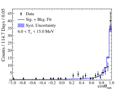
FIG. 4: Distribution of event directions with respect to solar direction for events with energy in $6.015.0$ MeV.

The upper five energy bins, $6.015.0$ MeV, were an extremely low background region for this analysis. There was very little background contamination from cosmogenically produced isotopes due primarily to depth of the detector. The comparatively high rate of backgrounds in the $5.06.0$ MeV bin comes primarily from decays of radioactive isotopes, such as radon, within the detector. Figure 4 shows the distribution in $\cos\theta_{\text{{sun}}}$ of events at energies above 6 MeV, illustrating the low background rate. In that energy region the best fit background rate was $0.25^{+0.09}_{-0.07}$ events/kt-day, much lower than the measured solar rate in that energy range, $1.03^{+0.13}_{-0.12}$ events/kt-day. For the region above 6 MeV, this is the lowest background elastic scattering measurement of solar neutrinos in a water Cherenkov detector.

IX Conclusion

Described here is the first measurement of the $\ce{{}^{8}B}$ solar neutrino flux as observed by the SNO+ detector in its water phase using 114.7 days of data. Our results are consistent with measurements from other experiments, and serve to provide continued monitoring of reactions within the core of the Sun.

The low rate of backgrounds above 6 MeV, in conjunction with the measured systematic uncertainties, allows an accurate measurement of the solar neutrino flux despite the limited size of the dataset. The low background rates at high energies come primarily from a low rate of cosmic-ray muons within the detector volume, and allows the measurement of other physical phenomena, including invisible nucleon decay Anderson et al. (2018) and potentially the local reactor anti-neutrino flux in the SNO+ water phase. The presence of radon backgrounds from the internal water limits this analysis at lower energies. In SNO+’s scintillator and tellurium loaded phases the internal radioactive backgrounds will be significantly reduced, allowing further measurements of solar neutrinos at lower energies.

References

- Bahcall et al. (2005) J. N. Bahcall, A. M. Serenelli, and S. Basu, The Astrophysical Journal Letters 621, L85 (2005).
- Cleveland et al. (1998) B. T. Cleveland et al., The Astrophysical Journal 496, 505 (1998).
- Abdurashitov et al. (2003) J. Abdurashitov et al., Nuclear Physics B - Proceedings Supplements 118, 39 (2003), proceedings of the XXth International Conference on Neutrino Physics and Astrophysics.
- Altmann et al. (2005) M. Altmann et al., Physics Letters B 616, 174 (2005).
- Hampel et al. (1999) W. Hampel et al., Physics Letters B 447, 127 (1999).
- Hirata et al. (1990) K. S. Hirata et al., International Astronomical Union Colloquium 121, 179–186 (1990).
- Bahcall and Ulrich (1988) J. N. Bahcall and R. K. Ulrich, Rev. Mod. Phys. 60, 297 (1988).
- Ahmad et al. (2001) Q. R. Ahmad et al. (SNO collaboration), Phys. Rev. Lett. 87, 071301 (2001).
- Ahmad et al. (2002) Q. R. Ahmad et al. (SNO collaboration), Phys. Rev. Lett. 89, 011301 (2002).
- Fukuda et al. (1998) Y. Fukuda et al. (Super-Kamiokande collaboration), Phys. Rev. Lett. 81, 1562 (1998).
- Fukuda et al. (2001) S. Fukuda et al. (Super-Kamiokande collaboration), Phys. Rev. Lett. 86, 5651 (2001).
- Bellini et al. (2010) G. Bellini et al. (Borexino collaboration), Phys. Rev. D 82, 033006 (2010).
- Abe et al. (2011) S. Abe et al. (KamLAND collaboration), Phys. Rev. C 84, 035804 (2011).
- Agostini et al. (2018) M. Agostini et al. (BOREXINO), Nature 562, 505 (2018).
- Bellini et al. (2014) G. Bellini et al. (Borexino collaboration), Phys. Rev. D 89, 112007 (2014).
- Gando et al. (2015) A. Gando et al. (KamLAND Collaboration), Phys. Rev. C 92, 055808 (2015).
- Andringa et al. (2016) S. Andringa et al. (SNO+ collaboration), Advances in High Energy Physics 2016 (2016).
- Boger et al. (2000) J. Boger et al. (SNO collaboration), Nucl. Instr. And Meth. A 449, 172 (2000).
- Bialek et al. (2016) A. Bialek et al., Nuclear Instruments and Methods in Physics Research Section A: Accelerators, Spectrometers, Detectors and Associated Equipment 827, 152 (2016).
- Agostinelli et al. (2003) S. Agostinelli et al., Nucl. Instr. And Meth. A 506, 250 (2003).
- Winter et al. (2006) W. T. Winter, S. J. Freedman, K. E. Rehm, and J. P. Schiffer, Phys. Rev. C 73, 025503 (2006).
- Bahcall et al. (1995) J. N. Bahcall, M. Kamionkowski, and A. Sirlin, Phys. Rev. D 51, 6146 (1995).
- Dragowsky et al. (2002) M. Dragowsky et al., Nucl. Instr. And Meth. A 481, 284 (2002).
- Anderson et al. (2018) M. Anderson et al. (SNO+ collaboration), (2018), arXiv:1812.05552 .
- Aharmim et al. (2010) B. Aharmim et al. (SNO Collaboration), Phys. Rev. C 81, 055504 (2010).
- Abe et al. (2016) K. Abe et al. (Super Kamiokande collaboration), Phys. Rev. D 94, 052010 (2016).
- Aharmim et al. (2013) B. Aharmim et al. (SNO Collaboration), Phys. Rev. C 88, 025501 (2013).
- Patrignani et al. (2016) C. Patrignani et al. (Particle Data Group), Chin. Phys C 40, 100001 (2016).
- Faulkner et al. (2006) P. J. W. Faulkner et al. (The GridPP collaboration), Journal of Physics G: Nuclear and Particle Physics 32, N1 (2006).
- Britton et al. (2009) D. Britton et al. (The GridPP collaboration), Philosophical Transactions of the Royal Society of London A: Mathematical, Physical and Engineering Sciences 367, 2447 (2009).