Inflation with mixed helicities and its observational imprint on CMB

Abstract

In the framework of effective field theories with prominent helicity-0 and helicity-1 fields coupled to each other via a dimension-3 operator, we study the dynamics of inflation driven by the helicity-0 mode, with a given potential energy, as well as the evolution of cosmological perturbations, influenced by the presence of a mixing term between both helicities. In this scenario, the temporal component of the helicity-1 mode is an auxiliary field and can be integrated out in terms of the time derivative of the helicity-0 mode, so that the background dynamics effectively reduces to that in single-field inflation modulated by a parameter $\beta$ associated to the coupling between helicity-0 and helicity-1 modes. We discuss the evolution of a longitudinal scalar perturbation $\psi$ and an inflaton fluctuation $\delta\phi$, and explicitly show that a particular combination of these two, which corresponds to an isocurvature mode, is subject to exponential suppression by the vector mass comparable to the Hubble expansion rate during inflation. Furthermore, we find that the effective single-field description corrected by $\beta$ also holds for the power spectrum of curvature perturbations generated during inflation. We compute the standard inflationary observables such as the scalar spectral index $n_{s}$ and the tensor-to-scalar ratio $r$ and confront several inflaton potentials with the recent observational data provided by Planck 2018. Our results show that the coupling between helicity-0 and helicity-1 modes can lead to a smaller value of the tensor-to-scalar ratio especially for small-field inflationary models, so our scenario exhibits even better compatibility with the current observational data.

I Introduction

Inflation Sta80 ; oldinf provides a causal mechanism for generating primordial density perturbations responsible for large-scale structures of the Universe oldper . Moreover, the temperature anisotropies observed in the Cosmic Microwave Background (CMB) are overall consistent with the prediction of the inflationary paradigm WMAP ; Planck2015 ; Planck2018 . It is anticipated that the possible detection of B-mode polarizations in the future will offer the opportunity to identify the origin of inflation.

The simplest candidate for inflation is a new scalar field $\phi$ beyond the Standard Model subject to a particular potential $V(\phi)$. As long as the field evolves slowly along a nearly flat potential, the primordial power spectra of scalar and tensor perturbations generated during inflation are close to scale-invariant Kolb . The deviation from scale invariance, characterized by the spectral index $n_{s}$ and the tensor-to-scalar ratio $r$, depends strongly on the assumption about the inflaton potential. Using the bounds of $n_{s}$ and $r$ constrained from the CMB data, one can distinguish between different inflationary models Martin ; TOKA ; PTEP ; Planck2015 ; Planck2018 ; Escudero:2015wba .

A cosmological accelerated expansion can be driven not only by a scalar field but also by a vector field. Indeed, the accelerated solutions were found in Ref. Koi08 ; Maroto1 in traditional vector-tensor theories, however they are generically plagued by instabilities vecins1 ; vecins2 ; vecins3 . In the so-called generalized Proca theories where an abelian vector field with broken $U(1)$ gauge symmetry has derivative self-interactions and nonminimal couplings to gravity Heisenberg ; Allys ; Jimenez16 (see also Ref. BGP ), the existence of a temporal vector component $A_{0}$ can give rise to de Sitter solutions. Indeed, the generalized Proca theories are very successful for describing the late-time cosmic acceleration GPcosmo1 ; GPcosmo2 .

On the other hand, there are also mechanisms for realizing the cosmic acceleration by using space-like vector fields Bento ; Armen . Naively this configuration is not compatible with an isotropic cosmological background, but the rotational invariance can be preserved by considering three orthogonal vector fields aligned with three spatial directions. Indeed, three vector fields $A^{a}_{\mu}$ nonminimally coupled to the Ricci scalar $R$ in the form $RA^{a}_{\mu}A^{a\mu}$ can lead to inflation vectorinf , but such accelerated solutions are plagued by either ghosts or Laplacian instabilities Peloso . Non-abelian gauge fields with $SU(2)$ gauge symmetry can be also the source for inflation without instabilities gaugeinf ; Soda , but the scalar spectral index $n_{s}$ and the tensor-to-scalar ratio $r$ are not compatible with the CMB data Namba ; Ads . There exists an inflationary scenario driven by a nonminimally coupled non-abelian gauge field Davydov , but the tensor perturbation is subject to ghost instabilities Jose .

Efforts have also been made to construct well-behaved inflationary models in the presence of vector fields but where, as in the standard case, the main source for the accelerated expansion is a scalar field $\phi$. It is of particular interest the case where this field is coupled to an abelian vector field $A_{\mu}$. It is known that, for this type of scenarios, a stable inflationary solution with an anisotropic hair exists for the coupling of the form $f^{2}(\phi)F_{\mu\nu}F^{\mu\nu}$, where $F_{\mu\nu}=\nabla_{\mu}A_{\nu}-\nabla_{\nu}A_{\mu}$ is the field strength tensor with a covariant derivative operator $\nabla_{\mu}$ aniinf . The same coupling has been often used for the generation of magnetic fields during inflation Turner ; Ratra , but in such cases the models need to be carefully constructed to avoid the back-reaction and strong-coupling problems Bamba ; Kanno ; Slava ; Fujita ; Mukoh .

Moreover, in the presence of a real scalar field $\phi$ and a vector field $A_{\mu}$ with derivative self-interactions and nonminimal couplings to gravity, the general action of scalar-vector-tensor (SVT) theories was recently constructed by keeping the equations of motion up to second order Heisenberg2 . In particular, the massive vector field with broken $U(1)$ gauge symmetry is relevant to the cosmological application. In this case, the vector perturbation is subject to exponential suppression by the mass of $A_{\mu}$.

Among the possible interactions between scalar and massive vector fields, and in particular for inflation, the coupling $A^{\mu}\nabla_{\mu}\phi$ is the simplest one modifying the inflaton velocity, $\dot{\phi}$, during the cosmic expansion. This interaction is not only prone to SVT theories but arises in many effective field theories as one of the lowest-order operator, once the involved broken gauge symmetries are compensated by the introduction of appropriate Stückelberg fields. In addition, the vector-field contribution to the total energy density during inflation is subdominant relative to the scalar potential $V(\phi)$, yet the modification to the inflaton velocity induced by the vector field can affect the primordial power spectra of scalar and tensor perturbations. See Ref. Heisenberg:2018vsk for a recent review on the systematic construction of modified gravity theories based on additional scalar, vector and tensor fields (see also Amendola:2012ys ).

For the aforementioned type of interaction, $A^{\mu}\nabla_{\mu}\phi$, there exists a longitudinal scalar perturbation, $\psi$, arising from $A_{\mu}$, besides the inflaton fluctuation $\delta\phi$ HKT18a ; KT18 ; HKT18b . This longitudinal perturbation contributes to the total curvature perturbation $\mathcal{R}$ in a nontrivial way. Therefore, the computation of the primordial power spectrum, incorporating both $\psi$ and $\delta\phi$, is not as straightforward as in the standard canonical case. In this paper, we address this problem and derive the standard inflationary observables such as $n_{s}$ and $r$ under the slow-roll approximation. We show that, as in the canonical case, one can relate these observables with slow-roll parameters but with a rescaling factor $\beta$ coming from the helicity-0 and helicity-1 mixing. Using these general expressions, we then confront several different inflaton potentials with the recent CMB data provided by the 2018 results from the Planck collaboration Planck2018 .

This paper is organized as follows. In Sec. II, we discuss the background inflationary dynamics and show that the system effectively reduces to that of a single-field inflation. In Sec. III, we revisit the primordial tensor power spectrum generated in our scenario and also study the evolution of vector perturbations during inflation. In Sec. IV, we investigate how the perturbations $\psi$ and $\delta\phi$ evolve during inflation and obtain the resulting power spectrum of total curvature perturbations. In Sec. V, we compute inflationary observables and test several inflaton potentials with the latest Planck 2018 data. Sec. VI is devoted to conclusions.

II Inflation with a scalar-vector coupling

In many effective field theories, mixings between different helicity modes, even with derivative interactions, arise in a natural way. In massive gravity and massive Proca theories, the decomposition of helicities yields interesting couplings among them deRham:2012ew ; Heisenberg ; Jimenez16 —this, in fact, motivated the construction of SVT theories Heisenberg2 . The particular mixing of the form $A^{\mu}\nabla_{\mu}\phi$ arises quite naturally and is a unique coupling that modifies the involved propagators of scalar and vector fields. As we will see below, one possible origin of this coupling is the standard Proca mass term, which modifies the property of propagator by the mass parameter.

Let us consider, for instance, the Lagrangian of the standard Proca field:

$$\mathcal{L}_{A_{\mu}}=-\frac{1}{4}F_{\mu\nu}F^{\mu\nu}-\frac{1}{2}M^{2}A_{\mu}A^{\mu}\,.$$ (1)

The existence of the mass term $M$ explicitly breaks the $U(1)$ gauge symmetry and therefore the massive spin-1 field propagates 3 degrees of freedom. Since the gauge invariance is just a redundancy, one can restore it by introducing a Stückelberg field $\phi$ via the field transformation

$$A_{\mu}\to A_{\mu}+\nabla_{\mu}\phi.$$ (2)

The initial Lagrangian for the massive spin-1 field (1) then modifies to

$$\mathcal{L}_{A_{\mu}}=-\frac{1}{4}F_{\mu\nu}F^{\mu\nu}-\frac{1}{2}M^{2}(A_{\mu}+\nabla_{\mu}\phi)(A^{\mu}+\nabla^{\mu}\phi)\,.$$ (3)

Notice that the kinetic term $-F_{\mu\nu}F^{\mu\nu}/4$ is not modified under this change of variables since it is gauge invariant. Here, the helicity-0 field $\phi$ represents the longitudinal mode of the massive vector field. Written in this form, the standard Proca theory is now invariant under the simultaneous transformations $A_{\mu}\to A_{\mu}+\nabla_{\mu}\theta$ and $\phi\to\phi-\theta$. After canonically normalizing the Stückelberg field $\phi\to\phi/M$, the Lagrangian becomes

$$\mathcal{L}_{A_{\mu}} = -\frac{1}{4}F_{\mu\nu}F^{\mu\nu}-\frac{1}{2}M^{2}A_{\mu}A^{\mu}-\frac{1}{2}\nabla_{\mu}\phi\nabla^{\mu}\phi$$ (4)

$$-MA^{\mu}\nabla_{\mu}\phi\,.$$

The last term is exactly the coupling we are interested in. This Lagrangian constitutes our low energy effective field theory.

In the following, we will consider a soft breaking of the shift symmetry of the helicity-0 mode and introduce a scalar potential $V(\phi)$ of the real scalar field $\phi$ for the purpose of realizing a successful inflationary scenario. Bear in mind that any UV completion will unavoidably introduce the breaking of global symmetry anyway. Our setup consists in an inflationary scenario in which the inflaton field $\phi$ has a derivative interaction with a massive vector field $A^{\mu}$ of the form $A^{\mu}\nabla_{\mu}\phi$, equivalent to that in Eq. (4). The inflationary period is mostly driven by the scalar potential $V(\phi)$, but the scalar-vector coupling modifies the dynamics of inflation and the primordial power spectra of cosmological perturbations. We then focus on the action 

$${\cal S} = \int d^{4}x\sqrt{-g}\Biggl{[}\frac{M_{\rm pl}^{2}}{2}R+F+X_{1}-V(\phi)$$ (5)

$$\qquad\qquad\quad~{}+\beta_{m}MX_{2}+\beta_{A}M^{2}X_{3}\Biggr{]}\,,$$

where $g$ is the determinant of a metric tensor $g_{\mu\nu}$, $M_{\rm pl}$ is the reduced Planck mass, $R$ is the Ricci scalar, and $F=-(1/4)F_{\mu\nu}F^{\mu\nu}$. The quantity $X_{1}$ is the scalar kinetic energy $X_{1}=-(1/2)\nabla_{\mu}\phi\nabla^{\mu}\phi$, while $X_{2}$ and $X_{3}$ are defined by

$$X_{2}=-\frac{1}{2}A^{\mu}\nabla_{\mu}\phi,\qquad X_{3}=-\frac{1}{2}A_{\mu}A^{\mu}\,.$$ (6)

In the last two terms of Eq. (5), $M$ is a positive constant (mass of the vector field) relevant to the mass scale of inflation, and $\beta_{m}$ and $\beta_{A}$ are dimensionless constants associated with the scalar-vector mixing and the vector mass, respectively.

To discuss the background dynamics of inflation, we consider the flat Friedmann-Lemaître-Robertson-Walker (FLRW) spacetime described by the line element $ds^{2}=-dt^{2}+a^{2}(t)\delta_{ij}dx^{i}dx^{j}$, where $a(t)$ is a time-dependent scale factor. The vector-field profile compatible with this metric is of the form $A_{\mu}=(A_{0}(t),0,0,0)$, with a time-dependent scalar field $\phi=\phi(t)$. The background equations of motion in full parity-invariant SVT theories were already derived in Refs. HKT18a ; KT18 . For the action (5), they are given by

$$3M_{\rm pl}^{2}H^{2}=\frac{1}{2}\dot{\phi}^{2}+V-\frac{1}{2}\beta_{A}M^{2}A_{0}^{2}\,,$$ (7)

$$-2M_{\rm pl}^{2}\dot{H}=\dot{\phi}^{2}+\frac{1}{2}\beta_{m}M\dot{\phi}A_{0}\,,$$ (8)

$$\ddot{\phi}+3H\dot{\phi}+V_{,\phi}+\frac{1}{2}M\beta_{m}\left(\dot{A}_{0}+3HA_{0}\right)=0\,,$$ (9)

$$A_{0}=-\frac{\beta_{m}}{2\beta_{A}M}\dot{\phi}\,,$$ (10)

where $H\equiv\dot{a}/a$ is the Hubble expansion rate, a dot represents a derivative with respect to cosmic time $t$, and $V_{,\phi}\equiv dV/d\phi$. From Eq. (10), we notice that the temporal vector component $A_{0}$ is simply proportional to $\dot{\phi}$. Substituting Eq. (10) into Eqs. (7), (8), and (9), we obtain

$$3M_{\rm pl}^{2}H^{2}=\frac{1}{2}\beta\dot{\phi}^{2}+V\,,$$ (11)

$$-2M_{\rm pl}^{2}\dot{H}=\beta\dot{\phi}^{2}\,,$$ (12)

$$\ddot{\phi}+3H\dot{\phi}+\frac{V_{,\phi}}{\beta}=0\,,$$ (13)

where we have defined

$$\beta\equiv 1-\frac{\beta_{m}^{2}}{4\beta_{A}}\,.$$ (14)

The coupling $\beta$ is different from 1 due to the mixing term $\beta_{m}$. This leads to the modified evolution of $\phi$ compared to the standard case ($\beta=1$).

In Refs. HKT18a ; KT18 , the authors derived conditions for the absence of ghost and Laplacian instabilities of linear cosmological perturbations in the small-scale limit. The propagation speeds of tensor, vector, and scalar perturbations are all equivalent to that of light for the theory given by the action (5). The no-ghost conditions of tensor and vector perturbations are trivially satisfied, while the scalar ghost is absent under the condition

$$q_{s}=\frac{M^{2}}{16}\left(4\beta_{A}-\beta_{m}^{2}\right)>0\,,$$ (15)

and hence $4\beta_{A}>\beta_{m}^{2}\geq 0$. Then, the coupling (14) lies in the range

$$0<\beta\leq 1\,.$$ (16)

From Eq. (13), the nonvanishing mixing term $\beta_{m}$ effectively leads to a faster inflaton velocity.

Employing the slow-roll approximations $\beta\dot{\phi}^{2}/2\ll V$ and $|\ddot{\phi}|\ll|3H\dot{\phi}|$ in Eqs. (11) and (13), it follows that

$$3M_{\rm pl}^{2}H^{2}\simeq V\,,$$ (17)

$$3H\dot{\phi}\simeq-\frac{V_{,\phi}}{\beta}\,.$$ (18)

The slow-roll parameter associated with the cosmic expansion rate is given by

$$\epsilon\equiv-\frac{\dot{H}}{H^{2}}\simeq\frac{\epsilon_{V}}{\beta}\,,$$ (19)

where we used Eq. (12), and defined

$$\epsilon_{V}\equiv\frac{M_{\rm pl}^{2}}{2}\left(\frac{V_{,\phi}}{V}\right)^{2}\,.$$ (20)

The existence of the nonvanishing mixing term $\beta_{m}$ breaks the relation $\epsilon\simeq\epsilon_{V}$ in standard inflation. The field value $\phi=\phi_{f}$ at the end of inflation can be derived by the condition $\epsilon(\phi_{f})=1$, i.e.,

$$\epsilon_{V}(\phi_{f})=\beta\,.$$ (21)

The number of e-foldings counted to the end of inflation is given by

$$N=\int_{\phi}^{\phi_{f}}\frac{H}{\dot{\tilde{\phi}}}d\tilde{\phi}\simeq\frac{\beta}{M_{\rm pl}^{2}}\int_{\phi_{f}}^{\phi}\frac{V}{V_{,\tilde{\phi}}}d\tilde{\phi}\,,$$ (22)

where, in the last approximate equality, we again used the slow-roll approximation. For smaller $\beta$, the number of e-foldings gets smaller with a given initial value of $\phi$. This is attributed to the fact that the inflaton velocity is effectively increased by the nonvanishing coupling $\beta_{m}$.

If we introduce a rescaled field $\varphi$ defined by

$$\frac{d\varphi}{d\phi}=\sqrt{\beta}\,,$$ (23)

then Eqs. (11), (12), (13) reduce, respectively, to

$$3M_{\rm pl}^{2}H^{2}=\frac{1}{2}\dot{\varphi}^{2}+V\,,$$ (24)

$$-2M_{\rm pl}^{2}\dot{H}=\dot{\varphi}^{2}\,,$$ (25)

$$\ddot{\varphi}+3H\dot{\varphi}+V_{,\varphi}=0\,.$$ (26)

This means that the background dynamics in the presence of $\phi$ and $A_{0}\propto\dot{\phi}$ is equivalent to the effective single-field dynamics driven by the scalar field $\varphi$. From Eq. (23), we have $\dot{\phi}=\dot{\varphi}/\sqrt{\beta}$, so the inflaton $\phi$ evolves faster than the rescaled field $\varphi$ for $\beta_{m}\neq 0$.

III Tensor and vector perturbations

In this section, we revisit the tensor power spectrum generated during inflation HKT18a ; KT18 and also discuss the evolution of vector perturbations in SVT theories given by the action (5).

III.1 Tensor perturbations

The perturbed line element containing intrinsic tensor modes $h_{ij}(t,x^{i})$ on the flat FLRW background is given by

$$ds_{t}^{2}=-dt^{2}+a^{2}(t)\left(\delta_{ij}+h_{ij}\right)dx^{i}dx^{j}\,,$$ (27)

where $h_{ij}$ obeys the transverse and traceless conditions $\nabla^{j}h_{ij}=0$ and ${h_{i}}^{i}=0$. From Eq. (3.2) of Ref. HKT18a , the second-order action of $h_{ij}$, for the theory given by Eq. (5), is the same as that in GR, i.e.,

$${\cal S}_{t}^{(2)}=\int dtd^{3}x\,\frac{a^{3}M_{\rm pl}^{2}}{8}\delta^{ik}\delta^{jl}\left[\dot{h}_{ij}\dot{h}_{kl}-\frac{1}{a^{2}}(\partial h_{ij})(\partial h_{kl})\right]\,,$$ (28)

where the symbol $\partial$ represents the spatial partial derivative. In Fourier space with the coming wavenumber $k$, the equation of motion of $h_{ij}$ is given by

$$\ddot{h}_{ij}+3H\dot{h}_{ij}+\frac{k^{2}}{a^{2}}h_{ij}=0\,.$$ (29)

Deep inside the Hubble radius ($k/a\gg H$), the tensor perturbation is in a Bunch-Davies vacuum state, whereas after the Hubble exit ($k/a<H$) during inflation, $h_{ij}$ soon approaches a constant. Taking into account two polarization states, the primordial tensor power spectrum (per unit logarithmic wavenumber interval) generated during inflation yields HKT18a

$${\cal P}_{t}=\frac{2H^{2}}{\pi^{2}M_{\rm pl}^{2}}\biggr{|}_{k=aH}\,,$$ (30)

which should be evaluated at the Hubble exit. By using the slow-roll approximation (17), Eq. (30) can be expressed in terms of $V$, as

$${\cal P}_{t}\simeq\frac{2V}{3\pi^{2}M_{\rm pl}^{4}}\biggr{|}_{k=aH}\,.$$ (31)

III.2 Vector perturbations

For the vector sector, we choose the perturbed line element in the flat gauge

$$ds_{v}^{2}=-dt^{2}+2V_{i}dtdx^{i}+a^{2}(t)\delta_{ij}dx^{i}dx^{j}\,,$$ (32)

where the vector perturbation $V_{i}(t,x^{i})$ obeys the transverse condition $\nabla^{i}V_{i}=0$. The spatial component of $A_{\mu}$ contains the intrinsic vector mode $Z_{i}$ and the longitudinal scalar perturbation $\psi$, such that

$$A_{i}=Z_{i}+\nabla_{i}\psi\,,$$ (33)

where $Z_{i}$ obeys the condition $\nabla^{i}Z_{i}=0$. In this section, we study the evolution of vector perturbations $Z_{i}$ during inflation, leaving the analysis of scalar mode $\psi$ for Sec. IV.

Without loss of generality, we can choose the components of $V_{i}$ and $Z_{i}$ in the forms $V_{i}=(V_{1}(t,z),V_{2}(t,z),0)$ and $Z_{i}=(Z_{1}(t,z),Z_{2}(t,z),0)$. After integrating out the nondynamical field $V_{i}$, the second-order action of vector perturbations reduces to HKT18a

$${\cal S}_{v}^{(2)}=\int dtd^{3}x\sum_{i=1}^{2}\frac{a}{2}\left[\dot{Z}_{i}^{2}-\frac{1}{a^{2}}\left(\partial Z_{i}\right)^{2}-\beta_{A}M^{2}Z_{i}^{2}\right]\,.$$ (34)

Then, in Fourier space, the dynamical perturbation $Z_{i}$ obeys

$$\ddot{Z}_{i}+H\dot{Z}_{i}+\left(\frac{k^{2}}{a^{2}}+\beta_{A}M^{2}\right)Z_{i}=0\,,$$ (35)

which can be written as

$$Z_{i}^{\prime\prime}+\left(k^{2}+a^{2}\beta_{A}M^{2}\right)Z_{i}=0\,,$$ (36)

where a prime represents the derivative with respect to the conformal time $\tau=\int a^{-1}dt$. For the modes satisfying the condition $k^{2}\gg a^{2}\beta_{A}M^{2}$, the perturbation is in a Bunch-Davies vacuum state characterized by $Z_{i}=e^{-ik\tau}/\sqrt{2k}$. On the other hand, after the mass term $a^{2}\beta_{A}M^{2}$ dominates over $k^{2}$ during inflation, we solve Eq. (35) for $Z_{i}$ under the conditions that $H={\rm constant}$ and that $k^{2}/a^{2}$ is negligible relative to $\beta_{A}M^{2}$. We then obtain the following solution

$$Z_{i}=A_{+}e^{\lambda_{+}t}+A_{-}e^{\lambda_{-}t}\,,$$ (37)

where $A_{\pm}$ are integration constants, and

$$\lambda_{\pm}=\frac{H}{2}\left[-1\pm\sqrt{1-\frac{4\beta_{A}M^{2}}{H^{2}}}\right]\,.$$ (38)

Since $\beta_{A}>0$, the vector mass term leads to the exponential suppression of $Z_{i}$ after the perturbation enters the region $k^{2}/a^{2}<\beta_{A}M^{2}$. The term in the square root of Eq. (38) becomes negative for $4\beta_{A}M^{2}>H^{2}$. Now, we would like to consider the case in which $M$ is of the same order as the Hubble expansion rate $H$ during inflation. Then, for the coupling

$$\beta_{A}={\cal O}(1)\,,$$ (39)

the condition $4\beta_{A}M^{2}>H^{2}$ is satisfied. In this case, the amplitude of $Z_{i}$ decreases as

$$|Z_{i}|\propto e^{-Ht/2}\,,$$ (40)

with damped oscillations. Then, the vector perturbation decays very fast once it enters the region $k^{2}/a^{2}<\beta_{A}M^{2}$. Since $\beta_{A}M^{2}$ is of the same order as $H^{2}$, this exponential suppression starts to occur around the same moment of Hubble exit ($k^{2}/a^{2}<H^{2}$).

In the following, we focus on the coupling $\beta_{A}$ of order 1. Then, the amplitude of vector perturbations at the end of inflation is completely negligible relative to those of tensor and scalar perturbations, so we can ignore the contributions of vector perturbations to the total primordial power spectrum.

IV Primordial scalar power spectrum generated during inflation

Let us proceed to the derivation of the scalar power spectrum generated in our model given by the action (5). In doing so, we begin with the perturbed line-element on the FLRW background in the flat gauge:

$$ds_{s}^{2}=-(1+2\alpha)\,dt^{2}+2\nabla_{i}\chi dt\,dx^{i}+a^{2}(t)\delta_{ij}dx^{i}dx^{j}\,,$$ (41)

where $\alpha$ and $\chi$ are scalar metric perturbations. We decompose the scalar field $\phi$ into the background and perturbed parts, as

$$\phi=\phi_{0}(t)+\delta\phi(t,x^{i})\,.$$ (42)

In the following, we omit the subscript “0” from the background value of $\phi$. The temporal component of $A^{\mu}$ is expressed in the form

$$A^{0}=-A_{0}(t)+\delta A(t,x^{i})\,,$$ (43)

whereas the spatial vector component $A_{i}$ contains the longitudinal scalar perturbation $\psi$ as Eq. (33).

The second-order action ${\cal S}_{s}^{(2)}$ of scalar perturbations was already computed in full parity-invariant SVT theories HKT18a . In our theories given by the action (5), we show the explicit form of ${\cal S}_{s}^{(2)}$ in Eq. (101) of Appendix A. Varying the action ${\cal S}_{s}^{(2)}$ with respect to $\alpha,\chi,\delta A$, we obtain the equations of motion for these nondynamical perturbations, see Eqs. (104)-(106). After integrating them out from the action, we are finally left with two dynamical real fields, $\psi$ and $\delta\phi$. In general, any real scalar field ${\cal X}$ can be expanded in Fourier series, as

$${\cal X}=\int\frac{d^{3}k}{(2\pi)^{3}}\left[{\cal X}_{k}(t)a({\bm{k}})e^{i{\bm{k}}\cdot{\bm{x}}}+{\cal X}^{*}_{k}(t)a^{\dagger}({\bm{k}})e^{-i{\bm{k}}\cdot{\bm{x}}}\right]\,,$$ (44)

where ${\bm{k}}$ is a coming wavenumber and ${\cal X}_{k}(t)$ is the mode function in Fourier space. For a quantized field ${\cal X}$, the coefficient $a({\bm{k}})$ and its Hermitian conjugate $a^{\dagger}({\bm{k}})$ correspond to annihilation and creation operators.

Thus, the second-order action for dynamical perturbations ${\cal X}^{t}=(\psi_{k},\delta\phi_{k})$ in Fourier space can be written as

$${\cal S}_{s}^{(2)}=\int dtd^{3}x\,a^{3}\left(\dot{\vec{\mathcal{X}}}^{t}{\bm{K}}\dot{\vec{\mathcal{X}}}-\frac{k^{2}}{a^{2}}\vec{\mathcal{X}}^{t}{\bm{G}}\vec{\mathcal{X}}-\vec{\mathcal{X}}^{t}{\bm{M}}\vec{\mathcal{X}}\right)\,,$$ (45)

where ${\bm{K}}$, ${\bm{G}}$, and ${\bm{M}}$ are $2\times 2$ matrices. The matrix ${\bm{M}}$ does not contain the $k^{2}$ term. We note that the term $\vec{\mathcal{X}}^{t}{\bm{B}}\dot{\vec{\mathcal{X}}}$ appearing in Ref. HKT18a has been absorbed into ${\bm{M}}$ after the integration by parts. The nonvanishing matrix components are given by 

$$K_{11}=\frac{k^{2}\beta_{A}M^{2}}{2(k^{2}+a^{2}\beta_{A}M^{2})}\,,\quad K_{12}=K_{21}=\frac{\beta_{m}}{2\beta_{A}M}K_{11}\,,$$

$$K_{22}=\frac{1}{2}-\frac{a^{2}\beta_{m}^{2}M^{2}}{8(k^{2}+a^{2}\beta_{A}M^{2})}\,,$$

$$G_{11}=\frac{\beta_{A}M^{2}}{2}\,,\quad G_{12}=G_{21}=\frac{\beta_{m}M}{4}\,,\quad G_{22}=\frac{1}{2}\,,$$

$$M_{22}=\frac{V_{,\phi\phi}}{2}-\frac{(1-\delta_{\phi}^{2})V_{,\phi}^{2}}{6M_{\rm pl}^{2}H^{2}}-\frac{(1+\delta_{\phi})^{4}V_{,\phi}^{4}}{324\beta H^{6}M_{\rm pl}^{4}}\,,$$ (46)

where we used the background Eqs. (11)-(13) to eliminate $\dot{H}$ and $\ddot{\phi}$. We also introduced the dimensionless quantity

$$\delta_{\phi}\equiv\frac{\beta\ddot{\phi}}{V_{,\phi}}=-\frac{3\beta H\dot{\phi}+V_{,\phi}}{V_{,\phi}}\,,$$ (47)

which is smaller than order 1 during inflation. The off-diagonal components $K_{12}$ and $G_{12}$ do not vanish for $\beta_{m}\neq 0$.

To study the evolution of perturbations $\psi_{k}$ and $\delta\phi_{k}$ in Fourier space, we introduce the following combination

$$\delta\chi_{k}\equiv\psi_{k}+\frac{\beta_{m}}{2\beta_{A}M}\delta\phi_{k}\,.$$ (48)

Varying the action (45) with respect to $\psi_{k}$ and using the properties that both $K_{12}/K_{11}$ and $G_{12}/G_{11}$ are equivalent to $\beta_{m}/(2\beta_{A}M)$, we obtain

$$\frac{1}{a^{3}}\frac{d}{dt}\left(a^{3}K_{11}\dot{\delta\chi}_{k}\right)+\frac{k^{2}}{a^{2}}G_{11}\delta\chi_{k}=0\,.$$ (49)

For $k^{2}/a^{2}\gg\beta_{A}M^{2}$, we have $K_{11}\to\beta_{A}M^{2}/2=G_{11}$ and hence Eq. (49) reduces to

$$\ddot{\delta\chi}_{k}+3H\dot{\delta\chi}_{k}+\frac{k^{2}}{a^{2}}\delta\chi_{k}=0\,.$$ (50)

This equation is of the same form as Eq. (29) for tensor perturbations, i.e., the equation of motion of a massless field. For the modes deep inside the Hubble radius ($k^{2}/a^{2}\gg H^{2}$), the canonically normalized field $v_{k}=\sqrt{2}a\delta\chi_{k}$ is in a Bunch-Davies vacuum state characterized by $v_{k}=e^{-ik\int dt/a}/\sqrt{2k}$. Since we are considering the coupling in Eq. (39) with $M\simeq H$ during inflation, the transition to another regime $k^{2}/a^{2}<\beta_{A}M^{2}$ occurs around the exit of Hubble radius.

For $k^{2}/a^{2}\ll\beta_{A}M^{2}$, we have $K_{11}\to k^{2}/(2a^{2})$, so Eq. (49) yields

$$\ddot{\delta\chi}_{k}+H\dot{\delta\chi}_{k}+\beta_{A}M^{2}\delta\chi_{k}=0\,,$$ (51)

which is of the same form as Eq. (35) after taking the same limit. On the quasi de Sitter background ($H\simeq{\rm constant}$), the solution to Eq. (51) is given by

$$\delta\chi_{k}=A_{+}e^{\lambda_{+}t}+A_{-}e^{\lambda_{-}t}\,,$$ (52)

where $\lambda_{\pm}$ are equivalent to those given in Eq. (38). Analogous to the intrinsic vector mode $Z_{i}$, the perturbation $\delta\chi_{k}$ starts to be exponentially suppressed after it enters the region $k^{2}/a^{2}<\beta_{A}M^{2}$.

For the coupling $\beta_{A}$ satisfying $4\beta_{A}M^{2}>H^{2}$, the amplitude of $\delta\chi_{k}$ decreases as $|\delta\chi_{k}|\propto e^{-Ht/2}$. Then, the perturbation $\delta\chi_{k}$ is vanishing small at the end of inflation, so we can set $\delta\chi_{k}\simeq 0$ in Eq. (48) and hence

$$\psi_{k}\simeq-\frac{\beta_{m}}{2\beta_{A}M}\delta\phi_{k}\,.$$ (53)

One can notice that, from Eq. (10), the relation between $\psi_{k}$ and $\delta\phi_{k}$ is analogous to that between $A_{0}$ and $\dot{\phi}$.

The only possibility for avoiding the above strong suppression is to consider the small coupling $\beta_{A}\ll 1$. In this case, there is a period characterized by $H^{2}>k^{2}/a^{2}>\beta_{A}M^{2}$ during which the perturbation $\delta\chi_{k}$ is temporally frozen with the value at Hubble radius crossing. However, after the perturbation enters the region $k^{2}/a^{2}<\beta_{A}M^{2}$, $\delta\chi_{k}$ starts to decay according to Eq. (52). It is possible to derive the solution to Eq. (51) even for the background where the scale factor evolves as $a\propto t^{p}$, where $p$ is a positive constant. In this case the resulting solution is given by $|\delta\chi_{k}|\propto t^{-p/2}$, so the suppression of $\delta\chi_{k}$ also occurs after inflation whenever $H^{2}$ drops below the order of $\beta_{A}M^{2}$.

Varying the action (45) with respect to $\delta\phi_{k}$, it follows that

$$\frac{1}{a^{3}}\frac{d}{dt}\left[a^{3}\left(K_{22}\dot{\delta\phi}_{k}+K_{12}\dot{\psi}_{k}\right)\right]+\frac{k^{2}}{a^{2}}\left(G_{22}\delta\phi_{k}+G_{12}\psi_{k}\right)$$

$$+M_{22}\delta\phi_{k}=0\,.$$ (54)

Now, we employ Eq. (48) and its time derivative to eliminate $\psi_{k}$ and $\dot{\psi}_{k}$ from Eq. (54). In doing so, we also resort to the fact that $\delta\chi_{k}$ obeys Eq. (49). Then, the contributions arising from $\delta\chi_{k}$ to Eq. (54) cancel out, so that

$$\frac{1}{a^{3}}\frac{d}{dt}\left(a^{3}\tilde{K}_{22}\dot{\delta\phi}_{k}\right)+\left(\frac{k^{2}}{a^{2}}\tilde{G}_{22}+M_{22}\right)\delta\phi_{k}=0\,,$$ (55)

where

$$\tilde{K}_{22}\equiv K_{22}-\frac{\beta_{m}}{2\beta_{A}M}K_{12}=\frac{\beta}{2}\,,$$ (56)

$$\tilde{G}_{22}\equiv G_{22}-\frac{\beta_{m}}{2\beta_{A}M}G_{12}=\frac{\beta}{2}\,.$$ (57)

Taking the limit $\beta\to 1$ in Eq. (55) with Eqs. (56) and (57), we recover the perturbation equation of $\delta\phi_{k}$ in standard single-field inflation.

We introduce the canonically normalized field $\delta\sigma_{k}$, as

$$\delta\sigma_{k}\equiv a\sqrt{\beta}\delta\phi_{k}\,.$$ (58)

Then, we can express Eq. (55) in the form

$$\delta\sigma_{k}^{\prime\prime}+\left(k^{2}-\frac{a^{\prime\prime}}{a}+\frac{2a^{2}M_{22}}{\beta}\right)\delta\sigma_{k}=0\,.$$ (59)

On the quasi de-Sitter background characterized by $H\simeq{\rm constant}$, the conformal time $\tau=\int a^{-1}dt$ is approximately given by $\tau\simeq-(1+\epsilon)/(aH)$. Applying the slow-roll approximation (17) to the mass term $M_{22}$ and picking up next-to-leading order terms in slow-roll in Eq. (59), we obtain

$$\delta\sigma_{k}^{\prime\prime}+\left[k^{2}-2(aH)^{2}\left(1+\frac{5\epsilon_{V}-3\eta_{V}}{2\beta}\right)\right]\delta\sigma_{k}=0\,,$$ (60)

where we used the relation (19) and introduced the second slow-roll parameter

$$\eta_{V}\equiv\frac{M_{\rm pl}^{2}V_{,\phi\phi}}{V}\,.$$ (61)

Neglecting the time variations of $\epsilon_{V}$ and $\eta_{V}$, the solution to Eq. (60), which recovers the Bunch-Davies vacuum state ($\delta\sigma_{k}=e^{-ik\tau}/\sqrt{2k}$) in the asymptotic past ($k\tau\to-\infty$), is given by

$$\delta\sigma_{k}=\frac{\sqrt{\pi|\tau|}}{2}e^{i(1+2\nu)\pi/4}H_{\nu}^{(1)}(k|\tau|)\,,$$ (62)

where $H_{\nu}^{(1)}(k|\tau|)$ is the Hankel function of first kind, and

$$\nu=\frac{3}{2}+\frac{3\epsilon_{V}-\eta_{V}}{\beta}\,.$$ (63)

Using the relations $H_{\nu}^{(1)}(k|\tau|)\to-(i/\pi)\Gamma(\nu)(k|\tau|/2)^{-\nu}$ for $k\tau\to 0$ and $\Gamma(3/2)=\sqrt{\pi}/2$, the solution for $\delta\phi_{k}$ long after the Hubble exit during inflation is

$$\delta\phi_{k}=i\frac{H(1-\epsilon)}{k^{3/2}\sqrt{2\beta}}\frac{\Gamma(\nu)}{\Gamma(3/2)}\left(\frac{k|\tau|}{2}\right)^{3/2-\nu}\,.$$ (64)

In the de-Sitter limit characterized by $\epsilon_{V}\to 0$ and $\eta_{V}\to 0$, the solution (64) reduces to $\delta\phi_{k}\to iH/(k^{3/2}\sqrt{2\beta})$.

We introduce the curvature perturbation in flat gauge incorporating both the field perturbations $\delta\phi_{k}$ and $\psi_{k}$, as HKT18b

$${\cal R}=-\frac{H(\dot{\phi}\delta\phi_{k}+M^{2}A_{0}\psi_{k})}{\dot{\phi}^{2}+M^{2}A_{0}^{2}}\,.$$ (65)

By using Eq. (10) and eliminating $\psi_{k}$ on account of Eq. (48), we can write Eq. (65) in the form

$${\cal R}={\cal R}_{\phi}+{\cal R}_{\chi}\,,$$ (66)

where

$${\cal R}_{\phi}=-\frac{H\delta\phi_{k}}{\dot{\phi}}\,,\qquad{\cal R}_{\chi}=\frac{2\beta_{m}\beta_{A}}{4\beta_{A}^{2}+\beta_{m}^{2}}\frac{HM\delta\chi_{k}}{\dot{\phi}}\,.$$ (67)

Since $\delta\chi_{k}$ is exponentially suppressed by the end of inflation, we only need to compute the power spectrum of ${\cal R}_{\phi}$. Taking Eq. (55) with the mass term $M_{22}$ given in Eq. (46), the perturbation ${\cal R}_{\phi}$ obeys

$$\frac{1}{a^{3}\epsilon}\frac{d}{dt}\left(a^{3}\epsilon\dot{\cal R}_{\phi}\right)+\frac{k^{2}}{a^{2}}{\cal R}_{\phi}=0\,.$$ (68)

In the large-scale limit ($k^{2}/a^{2}\to 0$), we obtain the following solution

$${\cal R}_{\phi}=c_{1}+c_{2}\int\frac{dt}{a^{3}\epsilon}\,,$$ (69)

where $c_{1}$ and $c_{2}$ are integration constants. In slow-roll inflation, the second term on the right hand side of Eq. (69) can be identified as a decaying mode. Then, ${\cal R}_{\phi}$ approaches the constant $c_{1}$ soon after the Hubble exit. Then, the primordial power spectrum of ${\cal P}_{{\cal R}_{\phi}}$ per unit logarithmic wavenumber interval can be computed at $k=aH$, as

$${\cal P}_{{\cal R}_{\phi}}\equiv\frac{k^{3}}{2\pi^{2}}\left|{\cal R}_{\phi}\right|^{2}=\frac{H^{4}}{4\pi^{2}\dot{\phi^{2}}\beta}\biggr{|}_{k=aH}\,,$$ (70)

where we used the leading-order solution of Eq. (64). Applying the slow-roll approximations (17)-(18) to Eq. (70) and neglecting the contribution from $\delta\chi_{k}$ to the total curvature perturbation ${\cal R}$, the resulting primordial scalar power spectrum is given by

$${\cal P}_{\cal R}\simeq\frac{\beta V^{3}}{12\pi^{2}M_{\rm pl}^{6}V_{,\phi}^{2}}\biggr{|}_{k=aH}\,.$$ (71)

In comparison with the canonical picture of single-field inflation, the coupling $\beta$ induces different behavior for the scalar power spectrum. Using the background field $\varphi$ defined by Eq. (23), the power spectrum (71) can be written in the form ${\cal P}_{\cal R}=V^{3}/(12\pi^{2}M_{\rm pl}^{6}V_{,\varphi}^{2})|_{k=aH}$. This means that, as long as the perturbation $\delta\chi_{k}$ is negligibly small compared to $\delta\phi_{k}$ at the end of inflation, the effective single-field description in terms of $\varphi$ also works for curvature perturbations.

V Observational signatures in CMB

In this section, we compute inflationary observables to confront our SVT theories with the CMB data of temperature anisotropies and study how they are modified by the presence of the coupling $\beta$.

V.1 Inflationary observables

In Sec. III, we showed that vector perturbations are exponentially suppressed relative to scalar and tensor perturbations at the end of inflation, so we neglect the contribution of vector modes to the inflationary power spectra. At the pivot wavenumber $k_{0}=0.05$ Mpc^-1, the amplitude of curvature perturbations constrained from Planck 2018 observations is Planck2018

$${\cal P}_{\cal R}=\frac{\beta V^{3}}{12\pi^{2}M_{\rm pl}^{6}V_{,\phi}^{2}}=2.1\times 10^{-9}\,.$$ (72)

The spectral indices of tensor and scalar perturbations are defined, respectively, by

$$n_{t} \equiv \frac{d\ln{\cal P}_{t}}{d\ln k}\biggr{|}_{k=aH}\,,$$ (73)

$$n_{s} \equiv 1+\frac{d\ln{\cal P}_{\cal R}}{d\ln k}\biggr{|}_{k=aH}\,.$$ (74)

From Eqs. (31) and (71), we obtain

$$n_{t} = -\frac{2\epsilon_{V}}{\beta}\,,$$ (75)

$$n_{s} = 1-\frac{1}{\beta}\left(6\epsilon_{V}-2\eta_{V}\right)\,,$$ (76)

where we used the slow-roll approximations (17)-(18). The tensor-to-scalar ratio is given by

$$r\equiv\frac{{\cal P}_{t}}{{\cal P}_{\cal R}}=\frac{16\epsilon_{V}}{\beta}=16\epsilon\,.$$ (77)

From Eqs. (75) and (77), the following consistency relation holds

$$r=-8n_{t}\,,$$ (78)

which is of the same form as that in standard single-field inflation. We study how the coupling $\beta$ modifies the observational prediction of $n_{s}$ and $r$. We show that this modification generally depends on the form of inflaton potentials.

V.2 Different inflaton potentials and Planck 2018 constraints

In the following, we consider three different inflaton potentials arising in (i) natural inflation, (ii) $\alpha$-attractors, and (iii) brane inflation. We also discuss whether these models can be consistent with the latest Planck 2018 data Planck2018 in presence of the scalar-vector mixing.

V.2.1 Natural inflation

In natural inflation natural , the potential is given by

$$V(\phi)=M^{2}M_{\rm pl}^{2}\left[1+\cos\left(\frac{\phi}{f}\right)\right]\,,$$ (79)

where $f$ is a mass scale associated with the shift symmetry. In this case, the observables (72), (76), and (77) reduce, respectively, to

$${\cal P}_{\cal R} = \frac{f_{\beta}^{2}M^{2}(1+x)^{2}}{12\pi^{2}M_{\rm pl}^{2}(1-x)}=2.1\times 10^{-9}\,,$$ (80)

$$n_{s} = 1-\frac{3-x}{f_{\beta}^{2}(1+x)}\,,$$ (81)

$$r = \frac{8(1-x)}{f_{\beta}^{2}(1+x)}\,,$$ (82)

where $f_{\beta}\equiv\sqrt{\beta}f/M_{\rm pl}$ and $x\equiv\cos(\phi/f)$. From Eq. (22), we obtain $N=f_{\beta}^{2}\ln[(1-x_{f})/(1-x)]$, so that

$$x=1-(1-x_{f})e^{-N/f_{\beta}^{2}}\,,$$ (83)

where $x_{f}=(1-2f_{\beta}^{2})/(1+2f_{\beta}^{2})$ is the value of $x$ at the end of inflation determined by the condition (21). Substituting Eq. (83) into Eqs. (81) and (82), it follows that $n_{s}$ and $r$ depend on $f_{\beta}$ and $N$. For a given $N$, these observables are functions of $f_{\beta}$ alone. Hence the theoretical curve in the $(n_{s},r)$ plane is the same as that in standard natural inflation. The only difference is that the coupling $f/M_{\rm pl}$ is now modified to $f_{\beta}=\sqrt{\beta}f/M_{\rm pl}$. From Planck 2015 data Planck2015 , the coupling is constrained to be ${\rm log}_{10}(f_{\beta})>0.84$ at 95 % CL, i.e.,

$$f>\frac{6.9M_{\rm pl}}{\sqrt{\beta}}\,.$$ (84)

As in the standard case, the trans-Planckian problem about the scale $f$ also persists for $\beta<1$. With given values of $f,\beta$, and $N$, the mass scale $M$ is known from the Planck normalization (80).

The recent Planck 2018 data combined with the data of B-mode polarizations available from the BICEP2/Keck field (BK14) and baryon acoustic oscillations (BAO) indicate that most of the theoretical values of $n_{s}$ and $r$ in natural inflation are outside of the 95 % CL observational contour, see Fig. 8 of Ref. Planck2018 . As shown above, this situation is not improved by the mixing term $\beta_{m}$ between inflaton and vector fields.

V.2.2 $\alpha$-attractors

The $\alpha$-attractor model alpha is given by the potential

$$V(\phi)=\frac{3}{4}\alpha_{c}M^{2}M_{\rm pl}^{2}\left[1-\exp\left(-\sqrt{\frac{2}{3\alpha_{c}}}\frac{\phi}{M_{\rm pl}}\right)\right]^{2}\,,$$ (85)

where $\alpha_{c}$ is a dimensionless constant . Starobinsky inflation Sta80 characterized by the Lagrangian $f(R)=R+R^{2}/(6M^{2})$ gives rise to the potential (85) with $\alpha_{c}=1$ after a conformal transformation to the Einstein frame. In the limit that $\alpha_{c}\to\infty$, the potential (85) reduces to that in chaotic inflation: $V(\phi)=M^{2}\phi^{2}/2$.

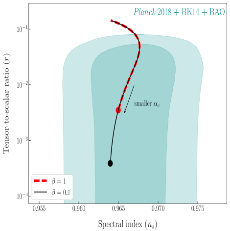
Figure 1: Observational constraints on $\alpha$-attractors in the $(n_{s},r)$ plane. The green contours represent the 68 % CL (inside) and 95 % CL (outside) boundaries derived by the joint data analysis of Planck 2018 $+$ BK14 $+$ BAO at $k=0.002$ Mpc^-1 Planck2018 . The red dashed and black thin solid lines correspond to the cases $\beta=1$ and $\beta=0.1$, respectively, with $N=55$ and $1\leq\alpha_{c}\leq 10^{6}$. The red and black circles represent Starobinsky inflation ($\alpha_{c}=1$) with $\beta=1$ and $\beta=0.1$, respectively.

For $\alpha$ attractors, the inflationary observables are

$${\cal P}_{\cal R} = \frac{3\alpha_{c}^{2}\beta M^{2}(1-y)^{4}}{128\pi^{2}M_{\rm pl}^{2}y^{2}}=2.1\times 10^{-9}\,,$$ (86)

$$n_{s} = 1-\frac{8y(1+y)}{3\alpha_{c}\beta(1-y)^{2}}\,,$$ (87)

$$r = \frac{64y^{2}}{3\alpha_{c}\beta(1-y)^{2}}\,,$$ (88)

where $y\equiv e^{-\sqrt{2/(3\alpha_{c})}\phi/M_{\rm pl}}$. The number of e-foldings is given by

$$N=\frac{3}{4}\alpha_{c}\beta\left(\frac{1}{y}-\frac{1}{y_{f}}+\ln\frac{y}{y_{f}}\right)\,,$$ (89)

where $y_{f}=(3\alpha_{c}\beta-2\sqrt{3\alpha_{c}\beta})/(3\alpha_{c}\beta-4)$ is the value of $y$ at the end of inflation.

For $\alpha_{c}<{\cal O}(10)$, $y$ is smaller than order 1 during inflation. In this case, the dominant contribution to $N$ is the first term in the parenthesis of Eq. (89), i.e., $y\simeq 3\alpha_{c}\beta/(4N)\ll 1$. Substituting this expression into Eqs. (87) and (88), we obtain

$$n_{s}\simeq 1-\frac{2}{N}\,,\qquad r\simeq\frac{12\alpha_{c}\beta}{N^{2}}\,.$$ (90)

While $n_{s}$ does not depend on $\beta$, the scalar-vector mixing ($\beta_{m}\neq 0$) leads to a smaller value for the tensor-to-scalar ratio compared to the case $\beta=1$. The Planck normalization (86) gives

$$M=1.3\times 10^{-5}M_{\rm pl}\sqrt{\beta}\left(\frac{55}{N}\right)\,,$$ (91)

so that $M$ decreases for smaller $\beta$.

For $\alpha_{c}\gg{\cal O}(10)$, $y$ approaches 1 with increasing $\alpha_{c}$. Expansion of Eq. (89) around $y=1$ shows that the number of e-foldings long before the end of inflation is approximately given by $N\simeq 3\alpha_{c}\beta(1-y)^{2}/8\gg 1$. In this regime, the observables (87) and (88) reduce to

$$n_{s}\simeq 1-\frac{2}{N}\,,\qquad r\simeq\frac{8}{N}\,,$$ (92)

which are equivalent to those in standard chaotic inflation driven by the potential $V(\phi)=M^{2}\phi^{2}/2$ TOKA . From Eq. (92), the coupling $\beta$ modifies neither $n_{s}$ nor $r$ for $\alpha_{c}\gg{\cal O}(10)$.

In Fig. 1, we plot the theoretical curves in the $(n_{s},r)$ plane for $\beta=1$ (red dashed) and $\beta=0.1$ (black thin solid) for $N=55$ and $1\leq\alpha_{c}\leq 10^{6}$. For $\alpha_{c}\gg{\cal O}(10)$, the observables converge to the values (92) irrespective of the coupling $\beta$. With decreasing $\alpha_{c}$, the difference of $r$ between the two different values of $\beta$ tends to be significant. In Starobinsky inflation ($\alpha_{c}=1$), for example, we have $r=3.9\times 10^{-4}$ for $\beta=0.1$. As estimated from Eq. (90), this is by one order of magnitude smaller than the value $r=3.5\times 10^{-3}$ for $\beta=1$. In both cases, the models are inside 68 % CL observational contour constrained from Planck 2018 $+$ BK14 $+$ BAO data. Interestingly, even if future observations place the upper limit of $r$ down to $10^{-3}$, the model with $\alpha_{c}=1$ can be still rescued by the coupling $\beta$.

As we observe in Fig. 1, the scalar spectral index $n_{s}$ for $\beta=0.1$ and $\alpha_{c}=1$ is slightly smaller than that for $\beta=1$ and $\alpha_{c}=1$. This reflects the fact that, in the latter case, the approximation $y\ll 1$ we used for the derivation of $n_{s}$ in Eq. (90) is not completely accurate. As the product $\alpha_{c}\beta$ decreases toward 0, the observables approach $n_{s}\to 1-2/N$ and $r\to 0$, which are favored in current CMB observations.

Since the coupling $\beta$ smaller than 1 can reduce the value of $r$, the bound on $\alpha_{c}$ is less stringent compared to the case $\beta=1$. For $\beta=1$ the observational upper limit is $\alpha_{c}<4.4\times 10$ (68 % CL), while, for $\beta=0.1$, the bound is loosened: $\alpha_{c}<4.2\times 10^{2}$ (68 % CL). Unless $\alpha_{c}$ is very much larger than 1 to approach the asymptotic values of $n_{s}$ and $r$ given by Eq. (92), the product $\alpha_{c}\beta$ is constrained to be

$$\alpha_{c}\beta\lesssim 40\,,$$ (93)

at 68 % CL. The main reason why $r$ is reduced by the mixing term $\beta_{m}$ is that the coupling $\beta$ leads to smaller $y\simeq 3\alpha_{c}\beta/(4N)$ (i.e., larger $\phi$) for $\alpha_{c}<{\cal O}(10)$. This effect overwhelms the coupling $\beta$ in the denominator of Eq. (88), so that $r$ has the dependence $r\propto\alpha_{c}\beta/N^{2}$. In other words, for $\beta<1$, we require that inflation occurs in the region where the potential is flatter relative to the case $\beta=1$ to acquire the same number of e-foldings. This effectively reduces the value of $r=16\epsilon$ for given $N$.

V.2.3 Brane inflation

Finally, we study brane inflation characterized by the effective potential

$$V(\phi)=M^{2}M_{\rm pl}^{2}\left[1-\left(\frac{\mu}{\phi}\right)^{p}+\cdots\right]\,,$$ (94)

where $p$ and $\mu$ are positive constants. The models arising from the setup of D-brane and anti D-brane configuration have the power $p=2$ branep=2 or $p=4$ branep=4a ; branep=4b . For the positivity of $V(\phi)$, we require that $z\equiv\phi/\mu>1$. We assume that inflation ends around $\phi\approx\mu$ before the additional terms denoted by the ellipsis in Eq. (94) contributes to the potential.

The observables (72), (76), and (77) reduce, respectively, to

$${\cal P}_{\cal R} = \frac{\beta M^{2}\mu^{2}(z^{p}-1)^{3}}{12\pi^{2}M_{\rm pl}^{4}p^{2}z^{p-2}}=2.1\times 10^{-9}\,,$$ (95)

$$n_{s} = 1-\frac{pM_{\rm pl}^{2}[2(p+1)z^{p}+p-2]}{\mu^{2}z^{2}(z^{p}-1)^{2}\beta}\,,$$ (96)

$$r = \frac{8p^{2}M_{\rm pl}^{2}}{\mu^{2}z^{2}(z^{p}-1)^{2}\beta}\,.$$ (97)

The number of e-foldings is given by

$$N\simeq\frac{\beta\mu^{2}[z^{2}(2z^{p}-p-2)+p]}{2M_{\rm pl}^{2}p(p+2)}\,,$$ (98)

where we used the fact that the value of $z$ at the end of inflation is $z_{f}\simeq 1$.

Since inflation occurs in the region $z^{p}\gg 1$, we pick up the dominant contributions to Eqs. (96), (97), and (98). Then we have $z^{p+2}\simeq M_{\rm pl}^{2}p(p+2)N/\beta\mu^{2}$, and

$$n_{s} \simeq 1-\frac{2(p+1)}{(p+2)N}\,,$$ (99)

$$r \simeq 8p^{2}\left(\frac{\beta\mu^{2}}{M_{\rm pl}^{2}}\right)^{\frac{p}{p+2}}\left[\frac{1}{p(p+2)N}\right]^{\frac{2(p+1)}{p+2}}\,,$$ (100)

which show that the $\beta$ dependence appears in $r$ but not in $n_{s}$. From Eq. (99), we obtain $n_{s}=1-3/(2N)$ for $p=2$ and $n_{s}=1-5/(3N)$ for $p=4$, so they are larger than $n_{s}$ in Eq. (90) of $\alpha$ attractors. From Eq. (100), the tensor-to-scalar ratio has the dependence $r\propto\beta^{1/2}/N^{3/2}$ for $p=2$ and $r\propto\beta^{2/3}/N^{5/3}$ for $p=4$. In the limit that $p\gg 1$, we have $n_{s}\simeq 1-2/N$ and $r\propto\beta/N^{2}$, so they have the same dependence of $N$ and $\beta$ as those in $\alpha$-attractors with $\alpha_{c}<{\cal O}(10)$. The scalar-vector mixing works to reduce the tensor-to-scalar ratio compared to the case $\beta=1$. Unlike $\alpha$-attractors in which the dependence of $r$ with respect to $\beta$ depends on $\alpha_{c}$, the reduction of $r$ induced by the coupling $\beta$ occurs irrespective of the values of $\mu$.

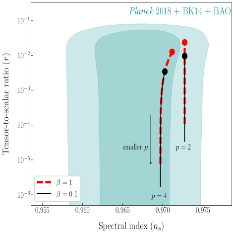
Figure 2: Observational constraints on brane inflation in the $(n_{s},r)$ plane for $p=2$ and $p=4$. The green contours are the same as those in Fig. 1. The red dashed and black thin solid lines represent the cases $\beta=1$ and $\beta=0.1$, respectively, with $N=55$ and $-1.5\leq{\rm log}_{10}(\mu/M_{\rm pl})\leq 1.0$. The red and black circles correspond to ${\rm log}_{10}(\mu/M_{\rm pl})=1.0$ with $\beta=1$ and $\beta=0.1$, respectively.

In Fig. 2, we plot the theoretical curves in the $(n_{s},r)$ plane for the brane inflation scenario with $\beta=1$ and $\beta=0.1$ for the mass range between $10^{-3/2}\leq\mu/M_{\rm pl}\leq 10$. We consider the models with two different powers: $p=2$ and $p=4$. For smaller $\mu$, $z$ gets larger and hence the approximate results (99)-(100) tend to be more accurate. As estimated from Eq. (99), the scalar spectral index is nearly constant, i.e., $n_{s}\simeq 0.9727$ for $p=2$ and $n_{s}\simeq 0.9697$ for $p=4$.

The red circle plotted on the line for $p=2$ of Fig. 2 corresponds to the model parameters $\beta=1$ and $\mu/M_{\rm pl}=10$, in which case the model is inside the 95 % CL observational contour with $r=2.35\times 10^{-2}$. From Eq. (100), the tensor-to-scalar ratio decreases for smaller values of $\beta$ and $\mu$. When $p=2$, $\beta=0.1$, $\mu/M_{\rm pl}=10$, the numerical value of $r$ is given by $9.53\times 10^{-3}$ —see the black circle on the line for $p=2$ of Fig. 2. The models with $\beta<1$ and $\mu\lesssim 10M_{\rm pl}$ are consistent with the current upper bound of $r$. For $p=2$, the scalar spectral index is between the 68 % CL and 95 % CL observational boundaries.

The model with $p=4$ gives rise to $n_{s}$ smaller than that for $p=2$, so the former model enters the 68% CL observational contour for $\mu\lesssim 10M_{\rm pl}$ and $\beta\leq 1$. The red circle shown on the line for $p=4$ of Fig. 2 corresponds to $\beta=1$ and $\mu/M_{\rm pl}=10$, in which case $r=1.25\times 10^{-2}$. For $\beta=0.1$, this value is reduced to $r=3.41\times 10^{-3}$. For smaller $\beta$ and $\mu$, the tensor-to-scalar ratio approximately decreases as $r\propto(\beta\mu^{2})^{2/3}$ for $p=4$.

We note that the increase of $r$ induced by the coupling $\beta~{}(<1)$ in the denominator of Eq. (97) is switched to the decrease of $r$ by the other term $z^{2+2p}\propto\beta^{-(2+2p)/(2+p)}$. Analogous to $\alpha$-attractors with $\alpha_{c}<{\cal O}(10)$, this behavior occurs in small-field inflation in which the variation of $\phi$ during inflation does not exceed the order of $M_{\rm pl}$. In $\alpha$-attractors with $\alpha_{c}\gg{\cal O}(10)$, which corresponds to large-field inflation, the decrease of $r$ induced by $\beta$ is not significant. In chaotic inflation (the limit $\alpha_{c}\to\infty$ in $\alpha$-attractors), both $\epsilon_{V}$ and $\eta_{V}$ are inversely proportional to $N$, in which case both $n_{s}$ and $r$ solely depend on $N$ but not on $\beta$. In small-field inflation, $\epsilon_{V}$ and $\eta_{V}$ have different $N$ dependence with $\epsilon_{V}\ll|\eta_{V}|$, in which case the explicit $\beta$ dependence appears in $r$.

VI Conclusions

This work was devoted to the study of prominent effective field theories with helicity-0 and helicity-1 fields in the presence of a dimension-3 operator that couples the two sectors. We have investigated the implications of this coupling for inflation driven by the helicity-0 mode with a given potential energy, paying particular attention to the evolution of cosmological perturbations. At the background level, the temporal component of helicity-1 mode, $A_{0}$, is just an auxiliary (nondynamical) field, so that it can be directly integrated out in terms of the time derivative of helicity-0 mode. In this way, the background dynamics resembles that of a single-field inflation modulated by a parameter $\beta$ associated with the coupling between the helicity-0 and helicity-1 modes.

We studied the evolution of longitudinal scalar perturbation $\psi_{k}$ in the presence of the inflaton fluctuation $\delta\phi_{k}$. The perturbation corresponding to the isocurvature mode is given by the combination $\delta\chi_{k}=\psi_{k}+\beta_{m}/(2\beta_{A}M)\delta\phi_{k}$. Existence of the vector-field mass $M$ comparable to the Hubble expansion rate during inflation leads to exponential suppression of $\delta\chi_{k}$ after the perturbation enters the region $k^{2}/a^{2}<\beta_{A}M^{2}$. We then explicitly showed that the power spectrum of the total curvature perturbation, $\mathcal{R}$, generated during inflation, corresponds to that of an effective single-field description also corrected by $\beta$. This is possible due to a similar relation between $\psi_{k}$ and $\delta\phi_{k}$ to that of $A_{0}$ and $\dot{\phi}$ at the background level, obtained in fact by the suppression of $\delta\chi_{k}$.

After deriving the power spectra of scalar and tensor perturbations generated during inflation, we computed their spectral indices $n_{s}$ and $n_{t}$ as well as the tensor-to-scalar ratio $r$ to confront our inflationary scenario with CMB observations. The mixing between helicity-0 and helicity-1 modes leads to modifications on $n_{s}$ and $r$ through the parameter $\beta$, with the same consistency relation $r=-8n_{t}$ as in the standard canonical case ($\beta=1$).

We computed the observables ${\cal P}_{\cal R}$, $n_{s}$, and $r$ for several inflaton potentials to explore the effect of coupling $\beta$ on CMB. For natural inflation, these observables reduce to those of the canonical case after the rescaling of the mass scale $f$. In small-field inflation like $\alpha$-attractors and brane inflation, however, the coupling $\beta~{}(<1)$ can lead to the suppression of $r=16\epsilon$ compared to the canonical case. This is attributed to the fact that, for smaller $\beta$, the total field velocity gets larger and hence inflation needs to start from a region in which the potential $V(\phi)$ is flatter to acquire the sufficient amount of $e$-foldings. Then, the tensor-to-scalar ratio decreases by the reduction of $\epsilon$ on scales relevant to observed CMB anisotropies.

In $\alpha$-attractors given by the potential (85), we showed that $n_{s}$ and $r$ are approximately given by $n_{s}\simeq 1-2/N$ and $r\simeq 12\alpha_{c}\beta/N^{2}$ for $\alpha_{c}<{\cal O}(10)$. This includes the Starobinsky inflation as a special case ($\alpha_{c}=1$). The coupling $\beta$ smaller than 1 leads to the suppression of $r$, so that the $\alpha$-attractor model exhibits even better compatibility with current CMB observations (see Fig. 1). For $\alpha_{c}<{\cal O}(10)$, we obtained the observational bound $\alpha_{c}\beta\lesssim 40$ (68 % CL) from the joint analysis based on the Planck 2018 $+$ BK14 $+$ BAO data sets. The similar suppression of $r$ and the better compatibility with observations have been also confirmed for brane inflation given by the potential (94). For $\beta<1$, the brane inflation models with $p=2$ and $p=4$ are inside the 95 % CL and 68 % CL observational contours, respectively, constrained from the Planck 2018 $+$ BK14 $+$ BAO data, see Fig. 2.

In this work, we focused on the simple mixing term $A^{\mu}\nabla_{\mu}\phi$ as a first step for computing primordial power spectra generated during inflation, but the further generalization of couplings between $\phi$ and $A^{\mu}$ is possible along the lines of Ref. Heisenberg2 . It will be also of interest to study potential signatures of such couplings in the CMB bispectrum as well as implications in the physics of reheating. Another direct implication worth studying is the improvement of standard inflationary models with respect to the de Sitter Swampland conjecture in the presence of this mixing term Obied:2018sgi . These interesting issues are left for future works.

Appendix A Second-order action for scalar perturbations (45)

In this Appendix, we show the details for the derivation of Eq. (45). In Eq. (5.4) of Ref. HKT18a , the second-order action ${\cal S}_{s}^{(2)}$ of scalar perturbations was derived in general SVT theories by choosing the flat gauge. For the specific theories given in this work by Eq. (5), we have

$${\cal S}_{s}^{(2)}=\int dtd^{3}x\,a^{3}\left({\cal L}_{s}^{\phi}+{\cal L}_{s}^{\rm GP}\right)\,,$$ (101)

where

$${\cal L}_{s}^{\phi} = \frac{1}{2}\dot{\delta\phi}^{2}-\frac{(\partial\delta\phi)^{2}}{2a^{2}}-\frac{1}{2}V_{,\phi\phi}\delta\phi^{2}-\left\{\dot{\phi}\left(2-\beta\right)\dot{\delta\phi}+V_{,\phi}\delta\phi\right\}\alpha+\dot{\phi}\beta\delta\phi\frac{\partial^{2}\chi}{a^{2}}-\frac{\beta_{m}M}{2}\left(\dot{\delta\phi}\delta A-\delta\phi\frac{\partial^{2}\psi}{a^{2}}\right),$$ (102)

$${\cal L}_{s}^{{\rm GP}} = -2HM_{\rm pl}^{2}\alpha\frac{\partial^{2}\chi}{a^{2}}+\frac{\beta_{m}^{2}\dot{\phi}^{2}}{2\beta_{A}^{2}M^{2}a^{2}}\left[(\partial\alpha)^{2}+\frac{\partial^{2}\delta A}{A_{0}}\alpha+\frac{\partial^{2}\dot{\psi}}{A_{0}}\alpha+\frac{(\partial\delta A)^{2}}{4A_{0}^{2}}-\frac{\dot{\psi}\partial^{2}\delta A}{2A_{0}^{2}}+\frac{(\partial\dot{\psi})^{2}}{4A_{0}^{2}}\right]$$ (103)

$$+\left[\dot{\phi}^{2}\left(\frac{1}{2}+\frac{3\beta_{m}^{2}}{8\beta_{A}}\right)-3H^{2}M_{\rm pl}^{2}\right]\alpha^{2}+\frac{\beta_{m}^{2}\dot{\phi}^{2}}{8\beta_{A}}\left(\frac{\delta A^{2}}{A_{0}^{2}}-4\alpha\frac{\delta A}{A_{0}}\right)-M^{2}\beta_{A}\frac{(\partial\psi)^{2}}{2a^{2}}\,.$$

Varying the action (101) with respect to $\alpha,\chi,\delta A$, we obtain the three constraint equations in Fourier space, respectively as

$$\dot{\phi}\left(1+\frac{\beta_{m}^{2}}{4\beta_{A}}\right)\dot{\delta\phi}+V_{,\phi}\delta\phi-\left[\dot{\phi}^{2}\left(1+\frac{3\beta_{m}^{2}}{4\beta_{A}}\right)-6H^{2}M_{\rm pl}^{2}\right]\alpha+\frac{\beta_{m}^{2}\dot{\phi}^{2}}{2\beta_{A}}\frac{\delta A}{A_{0}}$$

$$+\frac{k^{2}}{a^{2}}\left[\frac{\beta_{m}^{2}\dot{\phi}^{2}}{2\beta_{A}^{2}M^{2}}\left(\frac{\dot{\psi}}{A_{0}}+\frac{\delta A}{A_{0}}\right)-\frac{\beta_{m}^{2}\dot{\phi}^{2}}{\beta_{A}^{2}M^{2}}\alpha-2HM_{\rm pl}^{2}\chi\right]=0\,,$$ (104)

$$\dot{\phi}\left(1-\frac{\beta_{m}^{2}}{4\beta_{A}}\right)\delta\phi-2HM_{\rm pl}^{2}\alpha=0\,,$$ (105)

$$\beta_{m}M\dot{\delta\phi}+\frac{\beta_{m}^{2}\dot{\phi}^{2}}{2\beta_{A}}\left(\frac{2\alpha}{A_{0}}-\frac{\delta A}{A_{0}^{2}}\right)-\frac{k^{2}}{a^{2}}\frac{1}{A_{0}}\left[\frac{\beta_{m}^{2}\dot{\phi}^{2}}{2\beta_{A}^{2}M^{2}}\left(\frac{\dot{\psi}}{A_{0}}+\frac{\delta A}{A_{0}}\right)-\frac{\beta_{m}^{2}\dot{\phi}^{2}}{\beta_{A}^{2}M^{2}}\alpha\right]=0\,.$$ (106)

We solve Eqs. (104)-(106) for $\alpha,\chi,\delta A$ and substitute them into Eq. (101). Then, in Fourier space, we obtain the second-order action (45) for dynamical perturbations ${\cal X}^{t}=(\psi_{k},\delta\phi_{k})$ with the matrix components given by Eq. (46).

References

- (1) A. A. Starobinsky, Phys. Lett. B 91, 99 (1980).
- (2) R. Brout, F. Englert and E. Gunzig, Annals Phys. 115, 78 (1978); D. Kazanas, Astrophys. J. 241 L59 (1980); K. Sato, Mon. Not. R. Astron. Soc. 195, 467 (1981); Phys. Lett. 99B, 66 (1981); A. H. Guth, Phys. Rev. D 23, 347 (1981).
- (3) V. F. Mukhanov and G. V. Chibisov, JETP Lett. 33, 532 (1981); A. H. Guth and S. Y. Pi, Phys. Rev. Lett. 49 (1982) 1110; S. W. Hawking, Phys. Lett. B 115, 295 (1982); A. A. Starobinsky, Phys. Lett. B 117 (1982) 175; J. M. Bardeen, P. J. Steinhardt and M. S. Turner, Phys. Rev. D 28, 679 (1983).
- (4) G. Hinshaw et al. [WMAP Collaboration], Astrophys. J. Suppl. 208, 19 (2013) [arXiv:1212.5226 [astro-ph.CO]].
- (5) P. A. R. Ade et al. [Planck Collaboration], Astron. Astrophys. 594, A20 (2016) [arXiv:1502.02114 [astro-ph.CO]].
- (6) Y. Akrami et al. [Planck Collaboration], arXiv:1807.06211 [astro-ph.CO].
- (7) J. E. Lidsey, A. R. Liddle, E. W. Kolb, E. J. Copeland, Rev. Mod. Phys. 69, 373 (1997); D. H. Lyth and A. Riotto, Phys. Rept. 314, 1 (1999); B. A. Bassett, S. Tsujikawa and D. Wands, Rev. Mod. Phys. 78, 537 (2006).
- (8) J. Martin, C. Ringeval and V. Vennin, Phys. Dark Univ. 5-6, 75 (2014) [arXiv:1303.3787 [astro-ph.CO]].
- (9) S. Tsujikawa, J. Ohashi, S. Kuroyanagi and A. De Felice, Phys. Rev. D 88, 023529 (2013) [arXiv:1305.3044 [astro-ph.CO]].
- (10) S. Tsujikawa, PTEP 2014, no. 6, 06B104 (2014) [arXiv:1401.4688 [astro-ph.CO]].
- (11) M. Escudero, H. Ramírez, L. Boubekeur, E. Giusarma and O. Mena, JCAP 1602, 020 (2016) [arXiv:1509.05419 [astro-ph.CO]].
- (12) T. Koivisto and D. F. Mota, JCAP 0808, 021 (2008). [arXiv:0805.4229 [astro-ph]].
- (13) J. Beltran Jimenez and A. L. Maroto, Phys. Rev. D 80, 063512 (2009). [arXiv:0905.1245 [astro-ph.CO]].
- (14) J. Beltran Jimenez and A. L. Maroto, JCAP 0902, 025 (2009). [arXiv:0811.0784 [astro-ph]].
- (15) G. Esposito-Farese, C. Pitrou and J. P. Uzan, Phys. Rev. D 81, 063519 (2010). [arXiv:0912.0481 [gr-qc]].
- (16) P. Fleury, J. P. Beltran Almeida, C. Pitrou and J. P. Uzan, JCAP 1411, 043 (2014). [arXiv:1406.6254 [hep-th]].
- (17) L. Heisenberg, JCAP 1405, 015 (2014) [arXiv:1402.7026 [hep-th]].
- (18) E. Allys, P. Peter and Y. Rodriguez, JCAP 1602, 004 (2016). [arXiv:1511.03101 [hep-th]].
- (19) J. Beltran Jimenez and L. Heisenberg, Phys. Lett. B 757, 405 (2016). [arXiv:1602.03410 [hep-th]].
- (20) G. Tasinato, JHEP 1404, 067 (2014) [arXiv:1402.6450 [hep-th]]; G. Tasinato, Class. Quant. Grav. 31, 225004 (2014) [arXiv:1404.4883 [hep-th]]; L. Heisenberg, R. Kase and S. Tsujikawa, Phys. Lett. B 760, 617 (2016) [arXiv:1605.05565 [hep-th]]; J. Beltran Jimenez and T. S. Koivisto, Phys. Lett. B 756, 400 (2016) [arXiv:1509.02476 [gr-qc]]; J. Beltran Jimenez, L. Heisenberg and T. S. Koivisto, JCAP 1604, 046 (2016) [arXiv:1602.07287 [hep-th]].
- (21) A. De Felice, L. Heisenberg, R. Kase, S. Mukohyama, S. Tsujikawa and Y. l. Zhang, JCAP 1606, 048 (2016) [arXiv:1603.05806 [gr-qc]].
- (22) A. De Felice, L. Heisenberg, R. Kase, S. Mukohyama, S. Tsujikawa and Y. l. Zhang, Phys. Rev. D 94, 044024 (2016) [arXiv:1605.05066 [gr-qc]].
- (23) M. C. Bento, O. Bertolami, P. V. Moniz, J. M. Mourao and P. M. Sa, Class. Quant. Grav. 10, 285 (1993) [gr-qc/9302034].
- (24) C. Armendariz-Picon, JCAP 0407, 007 (2004) [astro-ph/0405267].
- (25) A. Golovnev, V. Mukhanov and V. Vanchurin, JCAP 0806, 009 (2008) [arXiv:0802.2068 [astro-ph]].
- (26) B. Himmetoglu, C. R. Contaldi and M. Peloso, Phys. Rev. Lett. 102, 111301 (2009) [arXiv:0809.2779 [astro-ph]]; B. Himmetoglu, C. R. Contaldi and M. Peloso, Phys. Rev. D 79, 063517 (2009) [arXiv:0812.1231 [astro-ph]].
- (27) A. Maleknejad and M. M. Sheikh-Jabbari, Phys. Lett. B 723, 224 (2013) [arXiv:1102.1513 [hep-ph]]; A. Maleknejad and M. M. Sheikh-Jabbari, Phys. Rev. D 84, 043515 (2011) [arXiv:1102.1932 [hep-ph]].
- (28) A. Maleknejad, M. M. Sheikh-Jabbari and J. Soda, Phys. Rept. 528, 161 (2013) [arXiv:1212.2921 [hep-th]].
- (29) R. Namba, E. Dimastrogiovanni and M. Peloso, JCAP 1311, 045 (2013) [arXiv:1308.1366 [astro-ph.CO]].
- (30) P. Adshead, E. Martinec and M. Wyman, JHEP 1309, 087 (2013) [arXiv:1305.2930 [hep-th]].
- (31) E. Davydov and D. Gal’tsov, Phys. Lett. B 753, 622 (2016) [arXiv:1512.02164 [hep-th]].
- (32) J. Beltran Jimenez, L. Heisenberg, R. Kase, R. Namba and S. Tsujikawa, Phys. Rev. D 95, 063533 (2017) [arXiv:1702.01193 [hep-th]].
- (33) M. a. Watanabe, S. Kanno and J. Soda, Phys. Rev. Lett. 102, 191302 (2009); [arXiv:0902.2833 [hep-th]]; A. E. Gumrukcuoglu, B. Himmetoglu and M. Peloso, Phys. Rev. D 81, 063528 (2010) [arXiv:1001.4088 [astro-ph.CO]]; M. a. Watanabe, S. Kanno and J. Soda, Prog. Theor. Phys. 123, 1041 (2010) [arXiv:1003.0056 [astro-ph.CO]]; J. Ohashi, J. Soda and S. Tsujikawa, JCAP 1312, 009 (2013) [arXiv:1308.4488 [astro-ph.CO]].
- (34) M. S. Turner and L. M. Widrow, Phys. Rev. D 37, 2743 (1988).
- (35) B. Ratra, Astrophys. J. 391, L1 (1992).
- (36) K. Bamba and J. Yokoyama, Phys. Rev. D 69, 043507 (2004) [astro-ph/0310824].
- (37) S. Kanno, J. Soda and M. a. Watanabe, JCAP 0912, 009 (2009) [arXiv:0908.3509 [astro-ph.CO]].
- (38) V. Demozzi, V. Mukhanov and H. Rubinstein, JCAP 0908, 025 (2009) [arXiv:0907.1030 [astro-ph.CO]].
- (39) T. Fujita and S. Mukohyama, JCAP 1210, 034 (2012) [arXiv:1205.5031 [astro-ph.CO]].
- (40) S. Mukohyama, Phys. Rev. D 94, 121302 (2016) [arXiv:1607.07041 [hep-th]].
- (41) L. Heisenberg, arXiv:1801.01523 [gr-qc].
- (42) L. Heisenberg, arXiv:1807.01725 [gr-qc].
- (43) L. Amendola et al. [Euclid Theory Working Group], Living Rev. Rel. 16, 6 (2013) [arXiv:1206.1225 [astro-ph.CO]]; L. Amendola et al., Living Rev. Rel. 21, no. 1, 2 (2018) [arXiv:1606.00180 [astro-ph.CO]]; E. J. Copeland, M. Sami and S. Tsujikawa, Int. J. Mod. Phys. D 15, 1753 (2006) [hep-th/0603057]; A. De Felice and S. Tsujikawa, Living Rev. Rel. 13, 3 (2010) [arXiv:1002.4928 [gr-qc]]; A. Joyce, B. Jain, J. Khoury and M. Trodden, Phys. Rept. 568, 1 (2015) [arXiv:1407.0059 [astro-ph.CO]].
- (44) L. Heisenberg, R. Kase and S. Tsujikawa, Phys. Rev. D 98, 024038 (2018) [arXiv:1805.01066 [gr-qc]].
- (45) R. Kase and S. Tsujikawa, JCAP 1811, 024 (2018) [arXiv:1805.11919 [gr-qc]].
- (46) L. Heisenberg, R. Kase and S. Tsujikawa, arXiv:1807.07202 [gr-qc] (Physical Review D to appear).
- (47) C. de Rham, G. Gabadadze, L. Heisenberg and D. Pirtskhalava, Phys. Rev. D 87, no. 8, 085017 (2013) [arXiv:1212.4128 [hep-th]].
- (48) K. Freese, J. A. Frieman and A. V. Olinto, Phys. Rev. Lett. 65, 3233 (1990); F. C. Adams, J. R. Bond, K. Freese, J. A. Frieman and A. V. Olinto, Phys. Rev. D 47, 426 (1993) [hep-ph/9207245].
- (49) R. Kallosh, A. Linde and D. Roest, JHEP 1311, 198 (2013) [arXiv:1311.0472 [hep-th]]; S. Ferrara, R. Kallosh, A. Linde and M. Porrati, Phys. Rev. D 88, no. 8, 085038 (2013) [arXiv:1307.7696 [hep-th]].
- (50) A. De Felice, S. Tsujikawa, J. Elliston and R. Tavakol, JCAP 1108, 021 (2011) [arXiv:1105.4685 [astro-ph.CO]].
- (51) J. Garcia-Bellido, R. Rabadan and F. Zamora, JHEP 0201, 036 (2002) [hep-th/0112147].
- (52) G. R. Dvali, Q. Shafi and S. Solganik, hep-th/0105203.
- (53) S. Kachru, R. Kallosh, A. D. Linde, J. M. Maldacena, L. P. McAllister and S. P. Trivedi, JCAP 0310, 013 (2003) [hep-th/0308055].
- (54) G. Obied, H. Ooguri, L. Spodyneiko and C. Vafa, arXiv:1806.08362 [hep-th]; P. Agrawal, G. Obied, P. J. Steinhardt and C. Vafa, Phys. Lett. B 784, 271 (2018) [arXiv:1806.09718 [hep-th]]; L. Heisenberg, M. Bartelmann, R. Brandenberger and A. Refregier, arXiv:1808.02877 [astro-ph.CO]; L. Heisenberg, M. Bartelmann, R. Brandenberger and A. Refregier, arXiv:1809.00154 [astro-ph.CO].