Permanence and Extinction for the Stochastic SIR Epidemic Model

Abstract

The aim of this paper is to study the stochastic SIR equation with general incidence functional responses and in which both natural death rates and the incidence rate are perturbed by white noises. We derive a sufficient and almost necessary condition for the extinction and permanence for SIR epidemic system with multi noises

$$\begin{cases}dS(t)=\big{[}a_{1}-b_{1}S(t)-I(t)f(S(t),I(t))\big{]}dt+\sigma_{1}S(t)dB_{1}(t)-I(t)g(S(t),I(t))dB_{3}(t),\\ dI(t)=\big{[}-b_{2}I(t)+I(t)f(S(t),I(t))\big{]}dt+\sigma_{2}I(t)dB_{2}(t)+I(t)g(S(t),I(t))dB_{3}(t).\end{cases}$$

Moreover, the rate of all convergences of the solution are also established. A number of numerical examples are given to illustrate our results.

Keywords. SIR model; Extinction; Permanence; Stationary Distribution; Ergodicity.

Subject Classification. 34C12, 60H10, 92D25.

1 Introduction

The epidemic models have a very long history and have been widely studied because of their importance in ecology. Such models were first introduced by Kermack and McKendrick in [11, 12] and recently, much attention has been devoted to analyzing, predicting the spread and designing controls of infectious diseases in host populations; see [2, 4, 5, 6, 8, 15, 16, 21, 22, 25, 27, 28, 29, 31]. One of the classical epidemic models is the SIR model which is suitable for modeling some diseases with permanent immunity such as rubella, whooping cough, measles, smallpox, etc. The SIR epidemic models consist of three groups of individuals: the susceptible, infected and recovered individuals, whose densities at the time $t$ are denoted by $S(t),I(t)$ and $R(t)$, respectively. The relationship between these quantities are in general described by the following equations

$$\begin{cases}dS(t)=\big{[}a_{1}-\mu_{S}S(t)-F(S(t),I(t))\big{]}dt,\\ dI(t)=\big{[}-(\mu_{I}+r)I(t)+F(S(t),I(t)\big{]}dt,\\ dR(t)=\big{[}-\mu_{R}R(t)+rI(t)\big{]}dt,\end{cases}$$ (1.1)

where $a_{1}>0$ is the recruitment rate of the population; $\mu_{S},\mu_{I},\mu_{R}>0$ are the death rates of the susceptible, infected and recovered individuals, respectively; $r>0$ is the recovery rate of the infected individuals and $F(S(t),I(t))$ is the incidence rate. To simplify the study, it has been noted that the dynamics of recovered individuals have no effect on the disease transmission dynamics. Thus, following the usual practice, the recovered individuals are removed from the formulation henceforth. Some kinds of the incidence rates are considered such as

• The Holling type II functional response (see e.g., [8]): $F(S,I)=\frac{\beta SI}{m_{1}+S}\cdot$

• The bilinear functional response (see e.g., [4, 31]): $F(S,I)=\beta SI$.

• The nonlinear functional response (see e.g., [25, 29]): $F(S,I)=\dfrac{\beta SI^{l}}{1+m_{2}I^{h}}\cdot$

• The Beddington-DeAngelis functional response (see e.g., [5, 6]): $F(S,I)=\dfrac{\beta SI}{1+m_{1}S+m_{2}I}\cdot$

For the deterministic SIR models with these incidence rates, the researchers have found the reproduction number $R_{0}$ which has the property: if $R_{0}<1$ then the disease free equilibrium point is locally asymptotically stale; in case $R_{0}>1$ we see that the disease point is unstable and there is a steady state, which is locally asymptotically stable.

However, it is well recognized that the environment is often affected by some random factors such as the temperature, the climate, the water resources, etc. Thus, it is important to consider the stochastic epidemic models. By these random effects, the death rates and the incidence rate are often perturbed by white noises. Many authors have considered the stochastic SIR models when the natural death rates are affected by white noises, i.e., $\mu_{S}\hookrightarrow\mu_{S}+\sigma_{1}\dot{B}_{1}(t),\mu_{I}+r\hookrightarrow\mu_{I}+r+\sigma_{2}\dot{B}_{2}(t)$, where $B_{i}(t),i=1,2$ are Brownian motions and the stochastic equation in general has the form (see e.g., [4, 6, 29])

$$\begin{cases}dS(t)=\big{[}a_{1}-b_{1}S(t)-I(t)f(S(t),I(t))\big{]}dt+\sigma_{1}S(t)dB_{1}(t),\\ dI(t)=\big{[}-b_{2}I(t)+I(t)f(S(t),I(t))\big{]}dt+\sigma_{2}I(t)dB_{2}(t),\\ \end{cases}$$

where, we have rewritten the coefficients: $b_{1}=\mu_{S},b_{2}=\mu_{I}+r$ and $F(S,I)=If(S,I)$ (compared with (1.1)). In an other motivation, some authors have studied the models, in which, the white noise acts on some special incidence functional responses, i.e., $f(s,i)\hookrightarrow f(s,i)+g(s,i)\dot{B}_{3}(t)$ and the stochastic equation becomes (see e.g., [1])

$$\begin{cases}dS(t)=\big{[}a_{1}-b_{1}S(t)-I(t)f(S(t),I(t))\big{]}dt-I(t)g(S(t),I(t))dB_{3}(t),\\ dI(t)=\big{[}-b_{2}I(t)+I(t)f(S(t),I(t))\big{]}dt+I(t)g(S(t),I(t))dB_{3}(t).\\ \end{cases}$$

By these motivations, the main aim of this paper is to generalize this problem by two ways. We study the stochastic SIR equation with more general incidence functional responses and in which, both natural death rates and the incidence rate are perturbed by white noises. Precisely, we consider the stochastic SIR equation as following

$$\begin{cases}dS(t)=\big{[}a_{1}-b_{1}S(t)-I(t)f(S(t),I(t))\big{]}dt+\sigma_{1}S(t)dB_{1}(t)-I(t)g(S(t),I(t))dB_{3}(t),\\ dI(t)=\big{[}-b_{2}I(t)+I(t)f(S(t),I(t))\big{]}dt+\sigma_{2}I(t)dB_{2}(t)+I(t)g(S(t),I(t))dB_{3}(t),\end{cases}$$ (1.2)

and provide a threshold number $R$ for the stochastic epidemic SIR model (1.2) that has the same properties as the reproduction number $R_{0}$ in the deterministic case. This means that when $R<1$ the number of the infected individuals $I(t)$ tends to zero with the exponential rate while the number of the susceptible individuals $S(t)$ converges exponentially to the solution on the boundary. In case of $R>1$, the solution has a unique invariant measure concentrated on $\mathbb{R}_{+}^{2,\circ}$ and the transition probability converges to the invariant measure in total variation norm with a polynomial of any degree rate. The ergodic property is also obtained in this case.

One of the main difficulties in studying this model is that the comparison theorem [9, Theorem 1.1, p.437] to compare the solution of (1.2) with the solution on boundary as in [4, 6] is no longer valid because there are complex white noises attended in the stochastic equation (1.2). Therefore, we can not approach the problem as usual and some new techniques must require here.

The rest of the paper is arranged as follows. Section 2 provides some preliminary results about the system and introduce the threshold $R$ to determine the permanence and extinction of the system. In Section 3, we derive the condition for the extinction of the system (1.2), which is equivalent to the case $R<1$ while section 4 focuses on the condition for permanence, corresponding to the case $R>1$. The last section is devoted to some numerical examples as well as discussing the obtained results in this paper.

2 Preliminary results and the threshold $R$

Throughout of this paper, we assume that the incidence rate and the diffusion term satisfy the following conditions.

Assumption 2.1.

Assume that

• $f,g$ are non-negative functions and $f(0,i)=0,g(0,i)=0\;\forall i\geq 0$,

• there exist positive constants $F,G,K$ such that

  $$\left|f(s_{1},i_{1})-f(s_{2},i_{2})\right| \leq F(\left|s_{1}-s_{2}\right|+\left|i_{1}-i_{2}\right|),$$

  $$\left|g(s_{1},i_{1})-g(s_{2},i_{2})\right| \leq G(\left|s_{1}-s_{2}\right|+\left|i_{1}-i_{2}\right|),$$

  $$\left|ig(s_{1},i)-ig(s_{2},i)\right| \leq G\left|s_{1}-s_{2}\right|\quad\text{and}\quad g(s,i)\leq K,$$

  for all $s_{1},s_{2},i_{1},i_{2},s,i\geq 0$.

We note that the bilinear incidence rate, the Beddington-DeAngelis incidence rate, the Holling type II functional response are special cases of this general incidence function.

2.1  The existence and uniqueness of the solution

Let $(\Omega,\mathcal{F},\{\mathcal{F}_{t}\}_{t\geq 0},\mathbb{P})$ be a complete probability space with the filtration $\{\mathcal{F}_{t}\}_{t\geq 0}$ satisfying the usual conditions and $B_{1}(t),B_{2}(t),$ $B_{3}(t)$ be mutually independent Brownian motions.

Theorem 2.1.

For any initial point $(u,v)\in\mathbb{R}_{+}^{2,\circ}:=\{(u^{\prime},v^{\prime})\in\mathbb{R}^{2}:u^{\prime},v^{\prime}>0\}$, there exists a unique global solution $(S_{u,v}(t),I_{u,v}(t)),t\geq 0$ of (1.2) with initial value $(S_{u,v}(0),I_{u,v}(0))=(u,v)$. Further, $(S_{u,v}(t),I_{u,v}(t))\in\mathbb{R}_{+}^{2,\circ}$ for all $t>0$.

Proof.

It is noted that although we have assumed $f(s,i)$ is Lipschitz continuous, the coefficient $if(s,i)$ in the system (1.2) is non-Lipschitz in general. Since the coefficients of the equation are locally Lipschitz continuous, there is a unique solution $(S_{u,v}(t),I_{u,v}(t))\in\mathbb{R}_{+}^{2,\circ}$ with the initial value $(u,v)\in\mathbb{R}_{+}^{2,\circ}$, defined on maximal interval $t\in[0,\tau_{e})$. We need to show $\tau_{e}=\infty$ a.s. Let us consider the Lyapunov function $V:\mathbb{R}_{+}^{2}\rightarrow\mathbb{R}_{+}$

$$V(s,i)=\left(s-C_{1}-C_{1}\ln{\frac{s}{C_{1}}}\right)+(i-1-\ln i)\;\;\;\;\;\text{where}\;\;\;\;\;C_{1}:=\frac{b_{2}}{F}\cdot$$

By directly calculating the differential operator $\mathcal{L}V(s,i)$, we have

$$\mathcal{L}V(s,i) =\left(1-\frac{C_{1}}{s}\right)\left(a_{1}-b_{1}s-if(s,i)\right)+\frac{C_{1}}{2s^{2}}\left(\sigma_{1}^{2}s^{2}+i^{2}g^{2}(s,i)\right)$$

$$\;\;\;+\left(1-\frac{1}{i}\right)\left(-b_{2}i+if(s,i)\right)+\frac{1}{2i^{2}}\left(\sigma_{2}^{2}i^{2}+i^{2}g^{2}(s,i)\right).$$

It follows from the assumption 2.1 that

$$f(s,i)=\left|f(s,i)-f(0,i)\right|\leq Fs\;\;\;\;\;\text{and}\;\;\;\;\;ig(s,i)=\left|ig(s,i)-ig(0,i)\right|\leq Gs.$$

Therefore, it is easily seen that

$$\mathcal{L}V(s,i) \leq C_{2}+\frac{C_{1}f(s,i)i}{s}+\frac{C_{1}g^{2}(s,i)i^{2}}{2s^{2}}+\frac{g^{2}(s,i)}{2}-b_{2}i$$

$$\leq C_{2}+\frac{C_{1}G^{2}}{2}+\frac{K^{2}}{2}+(C_{1}F-b_{2})i$$

$$=C_{2}+\frac{C_{1}G^{2}}{2}+\frac{K^{2}}{2},\quad\text{where}\;C_{2}=a_{1}+C_{1}b_{1}+\frac{C_{1}\sigma_{1}^{2}}{2}+b_{2}+\frac{\sigma_{2}^{2}}{2}.$$

As a result, $\mathcal{L}V(s,i)$ is bounded in $\mathbb{R}_{+}^{2,\circ}$. By using the same argument in the proofs in [14, Theorem 2.1, p. 994], we complete the proof of the theorem. ∎

2.2  Preliminary estimates about the expectation

Via Lyapunov functions we estimate moments of $S_{u,v}(t),I_{u,v}(t)$ that are shown in the following Lemma.

Lemma 2.1.

The following assertions hold:

• For any $0<p<\min\left\{\dfrac{2b_{1}}{\sigma_{1}^{2}},\dfrac{2b_{2}}{\sigma_{2}^{2}}\right\}$ and $\overline{p}>0$, there is a constants $Q_{1}$ such that

  $$\limsup\limits_{t\to\infty}\mathbb{E}\left[(S_{u,v}(t)+I_{u,v}(t))^{1+p}+(S_{u,v}(t)+I_{u,v}(t))^{-\overline{p}}\right]\leq Q_{1}\;\;\forall(u,v)\in\mathbb{R}_{+}^{2}.$$

• For any $\varepsilon>0$, $H>1$, $T>0$, there is $\overline{H}=\overline{H}(\varepsilon,H,T)$ such that

  $$\mathbb{P}\left\{\dfrac{1}{\overline{H}}\leq S_{u,v}(t)\leq\overline{H}\;\;\forall t\in[0,T]\right\}\geq 1-\varepsilon\;\;\text{if}\;\;\;(u,v)\in[H^{-1},H]\times[0;H],$$

  and

  $$\mathbb{P}\{0\leq S_{u,v}(t),I_{u,v}(t)\leq\overline{H}\;\;\forall t\in[0,T]\}\geq 1-\varepsilon\;\;\text{if}\;\;\;(u,v)\in[0,H]\times[0;H].$$

Proof.

Consider Lyapunov function $V_{1}(s,i)=(s+i)^{1+p}+(s+i)^{-\overline{p}}.$ By directly calculating the differential operator $\mathcal{L}V_{1}(s,i)$, we obtain

$$\mathcal{L}V_{1}(s,i)= (1+p)(s+i)^{p}(a_{1}-b_{1}s-b_{2}i)+\frac{p(1+p)}{2}(s+i)^{p-1}\Big{(}\sigma_{1}^{2}s^{2}+\sigma_{2}^{2}i^{2}\Big{)}$$

$$-\overline{p}(s+i)^{-\overline{p}-1}(a_{1}-b_{1}s-b_{2}i)+\frac{\overline{p}(1+\overline{p})}{2}(s+i)^{-\overline{p}-2}\Big{(}\sigma_{1}^{2}s^{2}+\sigma_{2}^{2}i^{2}\Big{)}$$

$$\leq (1+p)a_{1}(s+i)^{p}-(1+p)(s+i)^{p-1}\Big{[}(b_{1}-\dfrac{p}{2}\sigma_{1}^{2})s^{2}+(b_{2}-\dfrac{p}{2}\sigma_{2}^{2})i^{2}+(b_{1}+b_{2})si\big{]}$$

$$-\overline{p}a_{1}(s+i)^{-\overline{p}-1}+\overline{p}\left[\max\{b_{1},b_{2}\}+\frac{1+\overline{p}}{2}\max\{\sigma_{1}^{2},\sigma_{2}^{2}\}\right](s+i)^{-\overline{p}}.$$

Let $0<C_{3}<(1+p)\min\Big{\{}b_{1}-\dfrac{p}{2}\sigma_{1}^{2},b_{2}-\dfrac{p}{2}\sigma_{2}^{2},\dfrac{b_{1}+b_{2}}{2}\Big{\}}$. By some standard calculations, we get

$$C_{4}=\sup_{(s,i)\in\mathbb{R}^{2}_{+}\setminus\{(0,0)\}}\left\{\mathcal{L}V_{1}(s,i)+C_{3}V_{1}(s,i)\right\}<\infty.$$

That means

$$\mathcal{L}V_{1}(s,i)\leq C_{4}-C_{3}V_{1}(s,i).$$ (2.1)

Applying [17, Theorem 5.2, p.157] obtains the part (i) of Lemma.

Now, we move to the proof of the part (ii). By (2.1), there exist $h_{1}$,$h_{2}>0$ (see [7, Lemma 2.1, p. 45]) such that for all $(u,v)\in[0,H]\times[0,H]$

$$\mathbb{P}\Big{\{}0\leq S_{u,v}(t)\leq h_{1}\;\forall t\in[0,T]\Big{\}}\geq 1-\frac{\varepsilon}{2}\;\text{and}\;\mathbb{P}\Big{\{}0\leq I_{u,v}(t)\leq h_{2}\;\forall t\in[0,T]\Big{\}}\geq 1-\dfrac{\varepsilon}{2}.$$

Let

$$\Omega^{\prime}_{1}=\Big{\{}0\leq I_{u,v}(t)\leq h_{2}\;\forall t\in[0,T]\Big{\}},\;\;\Omega^{\prime}_{1}\;\text{may depend on}\;(u,v).$$

By exponential martingale inequality [17, Theorem 7.4, p. 44] we have $\mathbb{P}(\Omega^{\prime}_{2})\geq 1-\dfrac{\varepsilon}{2}$, where

$$\Omega^{\prime}_{2} =\left\{-\sigma_{1}B_{1}(t)+\int_{0}^{t}\dfrac{I_{u,v}(s)g(S_{u,v}(s),I_{u,v}(s))}{S_{u,v}(s)}dB_{3}(s)\right.$$

$$\hskip 14.22636pt\leq\left.\dfrac{\sigma_{1}^{2}t}{2}+\dfrac{1}{2}\int_{0}^{t}\dfrac{I^{2}_{u,v}(s)g^{2}(S_{u,v}(s),I_{u,v}(s))}{S^{2}_{u,v}(s)}ds+\ln\dfrac{2}{\varepsilon}\;\;\forall t\geq 0\right\},\;\;\Omega^{\prime}_{2}\;\text{may depend on}\;(u,v).$$

Applying Itô’s formula to the equation (1.2) yields that

$$\ln S_{u,v}(t)=\ln u+\int_{0}^{t}\dfrac{a_{1}}{S_{u,v}(s)}ds-\left(b_{1}+\dfrac{\sigma_{1}^{2}}{2}\right)t-\int_{0}^{t}\dfrac{I_{u,v}(s)f(S_{u,v}(s),I_{u,v}(s))}{S_{u,v}(s)}ds\\ \;\;\;-\dfrac{1}{2}\int_{0}^{t}\dfrac{I^{2}_{u,v}(s)g^{2}(S_{u,v}(s),I_{u,v}(s))}{S^{2}_{u,v}(s)}ds+\sigma_{1}B_{1}(t)-\int_{0}^{t}\dfrac{I_{u,v}(s)g(S_{u,v}(s),I_{u,v}(s))}{S_{u,v}(s)}dB_{3}(s).$$ (2.2)

For all $(u,v)\in[H^{-1},H]\times[0,H]$, $\omega\in\Omega^{\prime}_{1}\cap\Omega^{\prime}_{2}$ and $t\in[0,T]$, by the assumption 2.1 we have

$$\ln S_{u,v}(t) \geq\ln u-(b_{1}+\sigma_{1}^{2})t-F\int_{0}^{t}I_{u,v}(s)ds-G^{2}\int_{0}^{t}I^{2}_{u,v}(s)ds-\ln\dfrac{2}{\varepsilon}$$

$$\geq\ln H^{-1}-(b_{1}+\sigma_{1}^{2})T-h_{2}FT-h_{2}G^{2}T-\ln\dfrac{2}{\varepsilon}:=\ln h_{3}^{-1}$$

By setting $\overline{H}=\max\{1,h_{1},h_{2},h_{3}\}$ we complete the proof. ∎

Moreover, we note that $I_{u,v}(t)=0\;\forall t\geq 0$ a.s.  provided $I_{u,v}(0)=0$. Further, it follows [17, Theorem 2.9.3] and [30, Section 2.5] that the solution of (1.2) is homogeneous strong Markov and Feller process if provided that the coefficients are global Lipschitz. Therefore, by using the results in part (ii) of Lemma 2.1, we obtain from the local Lipschitz property of coefficients of (1.2) and a truncated argument that $(S_{u,v}(t),I_{u,v}(t))$ is homogeneous strong Markov and Feller process. The details of this truncated argument and this result can be found in [23, Theorem 5.1].

2.3  The threshold $R$

Consider the equation on boundary when the infected individuals are absent, i.e.,

$$d\varphi(t)=\big{(}a_{1}-b_{1}\varphi(t)\big{)}dt+\sigma_{1}\varphi(t)dB_{1}(t),\;\;\;\varphi(0)\geq 0.$$ (2.3)

We write $\varphi_{u}(t)$ for the solution of the equation (2.3) with the initial condition $\varphi(0)=u$. By solving the Fokker-Planck equation, the equation (2.3) has a unique stationary distribution with density $f^{*}$ given by

$$f^{*}(x)=\dfrac{b^{a}}{\Gamma(a)}x^{-(a+1)}e^{-\frac{b}{x}},\;x>0,$$ (2.4)

where $c_{1}=b_{1}+\dfrac{\sigma_{1}^{2}}{2},a=\dfrac{2c_{1}}{\sigma_{1}^{2}},b=\dfrac{2a_{1}}{\sigma_{1}^{2}}$ and $\Gamma(\cdot)$ is Gamma function. Our idea is to determine whether $I_{u,v}(t)$ converges to 0 or not by considering the Lyapunov exponent $\limsup_{t\to\infty}\dfrac{\ln I_{u,v}(t)}{t}$ when $I_{u,v}(t)$ is small. Using Itô’s formula gets

$$\dfrac{\ln I_{u,v}(t)}{t}= \dfrac{\ln v}{t}+\dfrac{\sigma_{2}B_{2}(t)}{t}+\dfrac{1}{t}\int_{0}^{t}g(S_{u,v}(s),I_{u,v}(s))dB_{3}(s)$$ (2.5)

$$-c_{2}+\dfrac{1}{t}\int_{0}^{t}\Big{(}f(S_{u,v}(s),I_{u,v}(s))-\dfrac{1}{2}g^{2}(S_{u,v}(s),I_{u,v}(s))\Big{)}ds,$$

where $c_{2}=b_{2}+\dfrac{\sigma_{2}^{2}}{2}.$ Intuitively, $\limsup_{t\to\infty}\frac{\ln I_{u,v}(t)}{t}<0$ implies $\lim_{t\to\infty}I_{u,v}(t)=0$ and when $I_{u,v}(t)$ is small then $S_{u,v}(t)$ is close to $\varphi_{u}(t)$ and therefore, when $t$ is sufficiently large we have

$$\dfrac{1}{t}\int_{0}^{t}\Big{(}f(S_{u,v}(s),I_{u,v}(s))-\dfrac{1}{2}g^{2}(S_{u,v}(s),I_{u,v}(s))\Big{)}ds\approx\dfrac{1}{t}\int_{0}^{t}\Big{(}f(\varphi_{u}(s),0)-\dfrac{1}{2}g^{2}(\varphi_{u}(s),0)\Big{)}ds.$$

By boundedness of $g(\cdot,\cdot)$; strong law of large numbers [26, Theorem 3.16, p.46] for $\varphi_{u}(t),$ from (2.5) we obtain that the Lyapunov exponent of $I_{u,v}(t)$ is approximated to

$$-c_{2}+\int_{0}^{\infty}\Big{(}f(x,0)-\dfrac{1}{2}g^{2}(x,0)\Big{)}f^{*}(x)dx:=\lambda.$$ (2.6)

Roughly speaking, if $\lambda>0$, whenever $I_{u,v}(t)$ is enough small, $\limsup_{t\to\infty}\frac{\ln I_{u,v}(t)}{t}\approx\lambda>0$ and it leads to $I_{u,v}(t)$ can not be very small in a long time. Conversely, when $\lambda<0$, if the solution starts from a initial point $(u,v)$, where v is sufficiently small then $\limsup_{t\to\infty}\frac{\ln I_{u,v}(t)}{t}\approx\lambda<0$ and which implies $I_{u,v}(t)\to 0$. Therefore, the remaining work is to investigate how the solution enters the region $\{(u,v):v\;\text{is sufficient small}\}$. However, that is just in intuition, the detailed proofs are very technical and complex and need to be carefully done.

Remark 1.

For $\lambda$ defined as in (2.6), $\lambda<0$ is equivalent to

$$R:=\dfrac{\int_{0}^{\infty}f(x,0)f^{*}(x)dx}{c_{2}+\int_{0}^{\infty}\frac{1}{2}g^{2}(x,0)f^{*}(x)dx}<1.$$ (2.7)

Therefore, we expect $R$ to be a threshold between the persistence and extinction of (1.2) as in the deterministic case. It is noted that since the conditions on $f(s,i)$, it is easy to see that $f(s,i)\leq Fs$ and thus,

$$\int_{0}^{\infty}\Big{(}f(x,0)-\dfrac{1}{2}g^{2}(x,0)\Big{)}f^{*}(x)dx\leq F\int_{0}^{\infty}xf^{*}(x)dx=\dfrac{Fa_{1}}{b_{1}}.$$

As a result, $\lambda,R$ are well-defined.

3 Extinction

Consider the case $R<1$ or equivalently, $\lambda<0$. We shall show that the number of the infected individuals $I_{u,v}(t)$ tends to zero with the exponential rate while the number of the susceptible individuals $S_{u,v}(t)$ converges to $\varphi_{u}(t)$. The problem here is that we can not apply the comparison theorem [9, Theorem 1.1, p.437] for $S_{u,v}(t)$ and $\varphi_{u}(t)$ to use a similar argument as in [4, 6].

Theorem 3.1.

Assume that $\lambda<0$. We also assume that the function $f(s,0)-\frac{1}{2}g^{2}(s,0)$ is monotonic. Then for any initial point $(u,v)\in\mathbb{R}_{+}^{2,\circ}$, the number of the infected individuals $I_{u,v}(t)$ tends to zero with the exponential rate $\lambda$ and the susceptible class $S_{u,v}(t)$ converges exponentially to the solution on boundary $\varphi_{u}(t)$. Precisely,

$$\limsup\limits_{t\to\infty}\dfrac{\ln I_{u,v}(t)}{t}=\lambda\text{\;a.s.\;}$$

and

$$\limsup\limits_{t\to\infty}\dfrac{\ln\left|S_{u,v}(t)-\varphi_{u}(t)\right|}{t}\leq\max\{\lambda,-c_{1}\}\text{\;a.s.\;}$$

In order to prove Theorem 3.1, we need some following auxiliary results.

Proposition 3.1.

For any $T,H>1,$ $\varepsilon>0,\theta>0$, there is a $\delta=\delta(H,T,\varepsilon,\theta)$ such that

$$\mathbb{P}\{\tau_{u,v}^{\theta}\geq T\}\geq 1-\varepsilon\;\;\forall\;(u,v)\in[0,H]\times(0,\delta],$$

where $\tau_{u,v}^{\theta}=\inf\{t\geq 0:I_{u,v}(t)>\theta\}.$

Proof.

By exponential martingale inequality [17, Theorem 7.4, p. 44], we have $\mathbb{P}(\Omega^{\prime\prime}_{1})\geq 1-\dfrac{\varepsilon}{2}$, where

$$\Omega^{\prime\prime}_{1}=\left\{\sigma_{2}B_{2}(t)+\int_{0}^{t}g(S_{u,v}(s),I_{u,v}(s))dB_{3}(s)\leq\dfrac{\sigma_{2}^{2}t}{2}+\dfrac{1}{2}\int_{0}^{t}g^{2}(S_{u,v}(s),I_{u,v}(s))ds+\ln\dfrac{2}{\varepsilon}\;\forall t\geq 0\right\},$$

$\Omega^{\prime\prime}_{1}$ may depend on $(u,v)$. In view of part (ii) Lemma 2.1, there exists $\overline{H}=\overline{H}(T,H,\varepsilon)$ such that $\mathbb{P}(\Omega^{\prime\prime}_{2})\geq 1-\dfrac{\varepsilon}{2}$, where

$$\Omega^{\prime\prime}_{2}=\{0\leq S_{u,v}(t),I_{u,v}(t)\leq\overline{H}\;\;\forall t\in[0,T]\},\;\;\Omega^{\prime\prime}_{2}\;\text{may depend on}\;(u,v).$$

Applying Itô’s formula to the equation (1.2) implies that

$$\ln I_{u,v}(t)=\ln v-c_{2}t+\int_{0}^{t}f(S_{u,v}(s),I_{u,v}(s))ds-\dfrac{1}{2}\int_{0}^{t}g^{2}(S_{u,v}(s),I_{u,v}(s))ds\\ +\sigma_{2}B_{2}(t)+\int_{0}^{t}g(S_{u,v}(s),I_{u,v}(s))dB_{3}(s).$$ (3.1)

Therefore, for any $(u,v)\in[0,H]\times(0,H]$ and $\omega\in\Omega^{\prime\prime}_{1}\cap\Omega^{\prime\prime}_{2}$ we have

$$\ln I_{u,v}(t)<\ln v-b_{2}t+t\big{(}2F\overline{H}+f(\overline{H},\overline{H})\big{)}+\ln\dfrac{2}{\varepsilon}\;\;\forall t\in[0,T].$$

Hence, we can choose a sufficiently small $\delta=\delta(H,T,\varepsilon,\theta)<H$ so that for all $(u,v)\in[0,H]\times(0,\delta]$ and $0\leq t\leq T$, $\ln I_{u,v}(t)<\ln\theta$. The proof is complete. ∎

Proposition 3.2.

For any $H,T>1$, $\varepsilon,\nu>0$, there exists $\theta>0$ such that for all $(u,v)\in[0,H]\times(0,\theta],$

$$\mathbb{P}\big{\{}\left|S_{u,v}(t)-\varphi_{u}(t)\right|\leq\nu\;\;\forall\;0\leq t\leq T\wedge\tau_{u,v}^{\theta}\big{\}}\geq 1-\varepsilon.$$

Proof.

First, in view of part (ii) in Lemma 2.1, there exists $\overline{H}$ such that

$$\mathbb{P}\{0\leq S_{u,v}(t),\varphi_{u}(t)\leq\overline{H}\;\forall t\in[0,T]\}\geq 1-\dfrac{\varepsilon}{2}\;\;\forall(u,v)\in[0,H]\times[0,H].$$ (3.2)

Second, by a same argument as in the proofs of [3, Lemma 3.2] or [17, Lemma 6.9], there exists a constant $C=C(H,\overline{H},T,\theta)$ satisfying

$$\begin{cases}\mathbb{E}\sup\limits_{0\leq t\leq T\wedge\tau_{u,v}^{\theta}\wedge\inf\{t\geq 0:S_{u,v}(t)\vee\varphi_{u}(t)>\overline{H}\}}\big{(}S_{u,v}(t)-\varphi_{u}(t)\big{)}^{2}\leq C,\\ C\to 0\;\text{ when}\;\theta\to 0.\end{cases}$$

Therefore, by virtue of Chebyshev’s inequality and (3.2), we can choose a sufficiently small constant $\theta$ such that

$$\mathbb{P}\{\left|S_{u,v}(t)-\varphi_{u}(t)\right|\leq\nu\;\;\forall 0\leq t\leq T\wedge\tau_{u,v}^{\theta}\}\geq 1-\varepsilon,\;\;\forall(u,v)\in[0,H]\times(0,\theta].$$

∎

The following lemma is a generalization of the law of iterated logarithm.

Lemma 3.1.

Let $W(t)$ be a standard Brownian motion and $\phi_{t}$ be a stochastic process, $\mathcal{F}_{t}-$ progressively measurable such that

$$P\left\{\int_{0}^{t}\phi_{s}^{2}\,ds<\infty\right\}=1\quad\text{ for all}\quad t>0.$$

Then for any $\varepsilon>0$ there exists a constant $q_{\varepsilon}$, independent of process $\phi$ such that

$$\mathbb{P}\left\{\bigg{|}\int_{0}^{t}\phi_{s}\,dW_{s}\bigg{|}\leq q_{\varepsilon}\sqrt{m(t)\ln(\left|m(t)\right|+1)}\right\}\geq 1-\varepsilon,$$

where $m(t)=\int_{0}^{t}\phi_{s}^{2}\,ds$.

Proof.

For simplifying notations, we set

$$M(t)=\int_{0}^{t}\phi_{s}\,dW_{s}\;;\;m(t)=\int_{0}^{t}\phi_{s}^{2}\,ds.$$

We define a family of stopping times $\tau_{1}(t)$ given by

$$\tau_{1}(t)=\begin{cases}\inf\{\;s\geq 0:m(s)>t\}\\ \infty\;\;\text{ if }\;\;t\geq m(\infty)=\lim_{t\uparrow\infty}m(t).\end{cases}$$

Applying [9, Theorem 7.2, p.92], on an extension $(\overset{\sim}{\Omega},\overset{\sim}{\mathcal{F}},\overset{\sim}{\mathbb{P}})$ of $(\Omega,\mathcal{F},\mathbb{P})$, there exists an $\overset{\sim}{\mathcal{F}}-$ Brownian motion $\mu(t)$ such that $\mu(t)=M(\tau_{1}(t)),$ $t\in[0,\infty).$ Consequently, we can represent $M(t)$ by an $\overset{\sim}{\mathcal{F}}-$ Brownian motion $\mu(t)$ and the stopping times $\tau_{1}(m(t))=t$, i.e.,

$$\int_{0}^{t}\phi_{s}\,dW_{s}=\mu(m(t)).$$

On the other hand, by virtues of the law of iterated logarithm we have

$$\limsup_{t\to\infty}\frac{|\mu(t)|}{\sqrt{2t\ln|\ln t|}}=1;\quad\limsup_{t\to 0}\frac{|\mu(t)|}{\sqrt{2t\ln|\ln t|}}=1\quad\text{ a.s.}$$

Therefore, the random variable $\Phi$ defined by

$$\Phi:=\sup_{0<t<\infty}\frac{|\mu(t)|}{\sqrt{t\big{(}|\ln t|+1\big{)}}}$$

is finite a.s. , i.e., $\mathbb{P}\{\Phi<\infty\}=1$ and the distribution of $\Phi$ does not depend on the process $(\phi_{t})$. The definition of $\Phi$ implies that

$$|\mu(t)|\leq\Phi\cdot\sqrt{t\big{(}|\ln t|+1\big{)}}.$$

Hence, one has

$$\bigg{|}\int_{0}^{t}\phi_{s}(\omega)\,dW_{s}\bigg{|}\leq\Phi\cdot\sqrt{m(t)\big{(}|\ln m(t)|+1\big{)}}.$$

Since $\Phi$ is finite  a.s.  and the distribution of $\Phi$ does not depend on $\phi$, for any $\varepsilon>0$ there exists $q_{\varepsilon}$ independent of $\phi$ such that $\mathbb{P}\{\Phi<q_{\varepsilon}\}\geq 1-\varepsilon.$ Lemma 3.1 is proved. ∎

Lemma 3.2.

For any $u\geq 0$, one has

$$\lim_{t\to\infty}\frac{\varphi_{u}(t)}{t}=0\text{\;a.s.\;}$$

Proof.

It is seen that as in Lemma 2.1, for $p<\frac{2b_{1}}{\sigma_{1}^{2}}$, we have $\mathcal{L}s^{\frac{1+p}{2}}\leq C_{4}-C_{3}s^{\frac{1+p}{2}}$, for some constants $C_{4},C_{3}$. Using this fact and Itô’s formula for $\varphi_{u}^{\frac{1+p}{2}}(t)$, we get that for all $n\in\mathbb{N}$

$$\sup_{t\in[n,n+1]}\varphi_{u}^{\frac{1+p}{2}}(t)\leq\varphi_{u}^{\frac{1+p}{2}}(n)+C_{4}+\sup_{t\in[n,n+1]}\int_{n}^{t}\frac{1+p}{2}\varphi_{u}^{\frac{1+p}{2}}(s)dB_{1}(s).$$

As a consequence, one has

$$\mathbb{E}\sup_{t\in[n,n+1]}\varphi_{u}^{1+p}(t)\leq 2(\varphi_{u}^{\frac{1+p}{2}}(n)+C_{4})^{2}+2\mathbb{E}\left(\sup_{t\in[n,n+1]}\int_{n}^{t}\frac{1+p}{2}\varphi_{u}^{\frac{1+p}{2}}(s)dB_{1}(s)\right)^{2}.$$ (3.3)

It is similar to Lemma 2.1 to obtain that

$$\sup_{t\in[0,\infty]}\mathbb{E}\left(\varphi_{u}^{1+p}(t)+\varphi_{u}^{\frac{1+p}{2}}(t)\right)\leq\overline{Q}_{1},$$

for some finite constant $\overline{Q}_{1}$. Which together with (3.3) and Burkholder-Davis-Gundy inequality give us that

$$\mathbb{E}\sup_{t\in[n,n+1]}\varphi_{u}^{1+p}(t)\leq 2\left(\overline{Q}_{1}+C_{4}\right)^{2}+8\overline{Q}_{1}=:\widehat{Q}.$$ (3.4)

For any $\varepsilon>0$, put $A_{n}=\Big{\{}\dfrac{\sup_{n\leq t\leq n+1}\varphi_{u}(t)}{n}\geq\varepsilon\Big{\}}$. From (3.4), we have $\mathbb{P}(A_{n})\leq(\varepsilon n)^{-(1+p)}\widehat{Q}$, which implies $\sum_{n=1}^{\infty}\mathbb{P}(A_{n})<\infty$. Hence, $\mathbb{P}\{A_{n}\text{ i.o.}\}=0$ by Borel-Cantelli lemma. In other word, $\limsup\limits_{n\to\infty}\dfrac{\sup_{n\leq t\leq n+1}\varphi_{u}(t)}{n}\leq\varepsilon$ a.s. Since $\varepsilon$ is arbitrary and $\varphi_{u}(t)>0$, the Lemma is proved. ∎

Proposition 3.3.

Assume that the assumption in Theorem 3.1 holds. For any $0<\varepsilon<\min\{\frac{1}{9},-\frac{\lambda}{9}\}$ and $H>1$, there exists $\widehat{\delta}=\widehat{\delta}(\varepsilon,H)\in(0,H^{-1})$ such that

$$\mathbb{P}\left\{\limsup_{t\to\infty}\left|\dfrac{\ln I_{u,v}(t)}{t}-\lambda\right|\leq\varepsilon\right\}\geq 1-8\varepsilon\;\forall(u,v)\in[H^{-1};H]\times(0;\widehat{\delta}].$$

Proof.

First, we consider the case the function $f(s,0)-\frac{1}{2}g^{2}(s,0)$ is non-decreasing. In what follows, although some sets $\Omega_{i}^{u,v}$ may not depend on $(u,v)$, we still use the superscript $(u,v)$ for the consistence of notations. Our idea in this proposition is to estimate simultaneously $\ln I_{u,v}(t)$ and the difference $\left|S_{u,v}(t)-\varphi_{u}(t)\right|$. To start, we need some following primary estimates. By definition of $\lambda$ and ergodicity of $\varphi_{H}(t)$ we obtain

$$-c_{2}+\lim_{t\to\infty}\dfrac{1}{t}\int_{0}^{t}f(\varphi_{H}(s),0)ds-\lim_{t\to\infty}\dfrac{1}{2t}\int_{0}^{t}g^{2}(\varphi_{H}(s),0)ds=\lambda\text{\;a.s.\;}$$

So, there exists $T_{1}=T_{1}(\varepsilon)>1$ such that $\mathbb{P}(\Omega_{1}^{u,v})\geq 1-\varepsilon$, where

$$\Omega_{1}^{u,v}=\left\{-c_{2}+\dfrac{1}{t}\int_{0}^{t}f(\varphi_{H}(s),0)ds-\dfrac{1}{2t}\int_{0}^{t}g^{2}(\varphi_{H}(s),0)ds\leq\lambda+\varepsilon,\;\forall t\geq T_{1}\right\}.$$

Furthermore, by exponential martingale inequality we have $\mathbb{P}(\Omega_{2}^{u,v})\geq 1-\varepsilon$, where

$$\Omega_{2}^{u,v} =\left\{\int_{0}^{t}g(S_{u,v}(s),I_{u,v}(s))dB_{3}(s)\leq\dfrac{K^{2}}{\varepsilon}\ln\dfrac{1}{\varepsilon}+\dfrac{\varepsilon}{2K^{2}}\int_{0}^{t}g^{2}(S_{u,v}(s),I_{u,v}(s))ds,\;\forall t\geq 0\right\}.$$

Since $\lim\limits_{t\to\infty}\dfrac{B_{2}(t)}{t}=0\text{\;a.s.\;}$, there is $T_{2}=T_{2}(\varepsilon)>1$ such that $\mathbb{P}(\Omega_{3}^{u,v})\geq 1-\varepsilon$ where

$$\Omega_{3}^{u,v}=\left\{\sigma_{2}\dfrac{B_{2}(t)}{t}<\dfrac{\varepsilon}{2}\;\forall t\geq T_{2}\right\}.$$

On the other hand, by Lipschitz continuity of $f,g$ and boundedness of $g$, we can choose $0<\nu=\nu(\varepsilon)<\min\Big{\{}1,\dfrac{\varepsilon}{2(F+KG)}\Big{\}}$ such that

$$\left|f(s_{1},i_{1})-f(s_{2},i_{2})\right|<\varepsilon\;\;\;\text{and}\;\;\;\left|\dfrac{1}{2}g^{2}(s_{1},i_{1})-\dfrac{1}{2}g^{2}(s_{2},i_{2})\right|<\varepsilon,$$

provided $\left|s_{1}-s_{2}\right|<\nu$ and $\left|i_{1}-i_{2}\right|<\nu$.

By Lemma 3.1, there exists $q_{\varepsilon}$, independent of $u,v$ such that $\mathbb{P}(\Omega_{4}^{u,v})\geq 1-\varepsilon$, where

$$\Omega_{4}^{u,v}:= \Big{\{}\left|\sigma_{1}B(t)\right|\leq q_{\varepsilon}\sqrt{t(\left|\ln t\right|+1)}\;\forall t\geq 0\Big{\}}$$

$$\bigcap\Bigg{\{}\left|\int_{T}^{t}e^{c_{1}s-\sigma_{1}B_{1}(s)}I_{u,v}(s)g(S_{u,v}(s),I_{u,v}(s))dB_{3}(s)\right|\leq q_{\varepsilon}\sqrt{n(t)(\left|\ln n(t)\right|+1)}\;\forall t\geq T\Bigg{\}},$$

and $T:=T_{1}\vee T_{2}$ and $n(t)=\int_{T}^{t}e^{2c_{1}s+2q_{\varepsilon}\sqrt{s(\left|\ln s\right|+1)}}I^{2}_{u,v}(s)g^{2}(S_{u,v}(s),I_{u,v}(s))ds$. To simplify notations we denote $q_{\varepsilon}(t):=q_{\varepsilon}\sqrt{t(\left|\ln t\right|+1)}$. It is clear that

$$\Phi_{1}(\varepsilon):=\sup_{t\geq 0}e^{-c_{1}t+q_{\varepsilon}(t)}e^{c_{1}T+q_{\varepsilon}(T)}\Big{(}1+\frac{K^{2}}{\varepsilon}\ln\frac{1}{\varepsilon}+\frac{\varepsilon}{2}\Big{)}T<\infty.$$

On the other hand, by Lemma 2.1 (ii), there exists $\overline{H}$ such that $\forall(u,v)\in[0,H]^{2}$, $\mathbb{P}(\Omega_{5}^{u,v})\geq 1-\varepsilon$ where

$$\Omega_{5}^{u,v}=\big{\{}0\leq S_{u,v}(t),I_{u,v}(t)\leq\overline{H}\;\forall t\in[0,T]\big{\}}.$$

In view of Proposition 3.2, there exists $\eta>0$ satisfying

$$\eta<\min\Big{\{}\nu,\dfrac{\nu}{2\Phi_{1}(\varepsilon)\big{(}2F\overline{H}+1\big{)}},\dfrac{\varepsilon}{2(F+KG)}\Big{\}}$$

such that $\forall(u,v)\in[H^{-1};H]\times(0;\eta],$ $\mathbb{P}(\Omega_{6}^{u,v})\geq 1-\varepsilon$ where

$$\Omega_{6}^{u,v}=\left\{\left|S_{u,v}(t)-\varphi_{u}(t)\right|<\nu\;\forall t\leq T\wedge\tau_{u,v}^{\eta}\right\}\;\text{and}\;\tau_{u,v}^{\eta}=\inf\{t\geq 0:I_{u,v}(t)>\eta\}.$$

We also set $\xi_{u,v}^{\nu}=\inf\{t\geq 0:\left|S_{u,v}(t)-\varphi_{u}(t)\right|>\nu\}$ and $\zeta_{u,v}:=\xi_{u,v}^{\nu}\wedge\tau_{u,v}^{\eta}$. By virtue of Proposition 3.1, there exists $0<\delta<\min\{H^{-1},\eta\}$ such that $\forall(u,v)\in[H^{-1};H]\times(0;\delta]$, $\mathbb{P}(\Omega_{7}^{u,v})\geq 1-\varepsilon,$ where $\Omega_{7}^{u,v}=\big{\{}\tau_{u,v}^{\eta}\geq T\big{\}}.$ Therefore, for all $(u,v)\in[H^{-1};H]\times(0;\delta]$, $\omega\in\cap_{i=1}^{7}\Omega_{i}^{u,v}$ we have $\zeta_{u,v}\geq T$.

Now, following the idea introduced at the beginning, we will estimate simultaneously $\ln I_{u,v}(t)$ and the difference $\left|S_{u,v}(t)-\varphi_{u}(t)\right|$. It follows from (3.1) that $\forall(u,v)\in[H^{-1},H]\times(0,\delta]$ we have in $\cap_{i=1}^{7}\Omega_{i}^{u,v}$

$$\ln I_{u,v}(t)=\ln v-c_{2}t+\int_{0}^{t}\left(f(\varphi_{H}(s),0)-\dfrac{1}{2}g^{2}(\varphi_{H}(s),0)\right)ds$$ (3.5)

$$\;\;\;\;\;+\int_{0}^{t}\Big{(}f(\varphi_{u},0)-\dfrac{1}{2}g^{2}(\varphi_{u}(s),0)-f(\varphi_{H}(s),0)+\dfrac{1}{2}g^{2}(\varphi_{H}(s),0)\Big{)}ds$$

$$\;\;\;\;\;+\int_{0}^{t}\Big{(}f(S_{u,v}(s),0)-f(\varphi_{u}(s),0)\Big{)}ds+\dfrac{1}{2}\int_{0}^{t}\left(g^{2}(\varphi_{u}(s),0)-g^{2}(S_{u,v}(s),0)\right)ds$$

$$\;\;\;\;\;+\int_{0}^{t}\Big{(}f(S_{u,v}(s),I_{u,v}(s))-f(S_{u,v},0)\Big{)}ds+\dfrac{1}{2}\int_{0}^{t}\left(g^{2}(S_{u,v}(s),0)-g^{2}(S_{u,v}(s),I_{u,v}(s))\right)ds$$

$$\;\;\;\;\;+\int_{0}^{t}g(S_{u,v}(s),I_{u,v}(s))dB_{3}(s)+\sigma_{2}B_{2}(t)\leq\ln v+\dfrac{K^{2}}{\varepsilon}\ln\dfrac{1}{\varepsilon}+(\lambda+6\varepsilon)t\;\;\forall t\in[T,\zeta_{u,v}],$$

where we have used the facts $\varphi_{u}(t)\leq\varphi_{H}(t)\text{\;a.s.\;}\forall t\geq 0,u\in[H^{-1},H]$ and the non-decreasing property of $f(s,0)-\dfrac{1}{2}g^{2}(s,0)$. Therefore, for all $(u,v)\in[H^{-1},H]\times(0,\delta]$, $\omega\in\cap_{i=1}^{7}\Omega_{i}^{u,v}$ we get

$$I_{u,v}(t)\leq v\varepsilon^{-\frac{K^{2}}{\varepsilon}}e^{\left(\lambda+6\varepsilon\right)t}\;\;\forall t\in[T,\zeta_{u,v}].$$ (3.6)

To proceed, we will estimate the difference $\left|S_{u,v}(t)-\varphi_{u}(t)\right|$. By using Itô’s formula and variation of constant formula, we get from (1.2) and (2.3) that

$$S_{u,v}(t)-\varphi_{u}(t) =e^{-c_{1}t+\sigma_{1}B_{1}(t)}\int_{0}^{t}e^{c_{1}s-\sigma_{1}B_{1}(s)}I_{u,v}(s)f(S_{u,v}(s),I_{u,v}(s))ds$$ (3.7)

$$\quad+e^{-c_{1}t+\sigma_{1}B_{1}(t)}\int_{0}^{t}e^{c_{1}s-\sigma_{1}B_{1}(s)}I_{u,v}(s)g(S_{u,v}(s),I_{u,v}(s))dB_{3}(s)$$

$$:=A_{1}^{u,v}(t)+A_{2}^{u,v}(t).$$

In the next paragraph, we are going to estimate $A_{1}^{u,v}(t),A_{2}^{u,v}(t)$.

A consequence of Lemma 2.3 is that there is $\Omega_{8}^{u}$ satisfying $\mathbb{P}(\Omega_{8}^{u})\geq 1-\varepsilon$, and $L_{1}$ (independent of $u$) such that for any $u\in[H^{-1},H]$, $\omega\in\Omega_{8}^{u}$, one has $\varphi_{u}(t)\leq L_{1}e^{\varepsilon t}.$ By direct calculations, from (3.6) and the assumption 2.1 we obtain that $\forall(u,v)\in[H^{-1},H]\times(0,\delta],\omega\in\cap_{i=1}^{8}\Omega_{i}^{u,v},t\geq T$

$$\big{|} A_{1}^{u,v}(t\wedge\zeta_{u,v})\big{|}\leq e^{-c_{1}(t\wedge\zeta_{u,v})+\sigma_{1}B_{1}(t\wedge\zeta_{u,v})}\int_{0}^{T}e^{c_{1}s-\sigma_{1}B_{1}(s)}I_{u,v}(s)f(S_{u,v}(s),I_{u,v}(s))ds$$

$$\quad+e^{-c_{1}(t\wedge\zeta_{u,v})+\sigma_{1}B_{1}(t\wedge\zeta_{u,v})}\int_{T}^{t\wedge\zeta_{u,v}}e^{c_{1}s-\sigma_{1}B_{1}(s)}I_{u,v}(s)f(S_{u,v}(s),I_{u,v}(s))ds$$

$$\leq 2\eta F\overline{H}e^{-c_{1}(t\wedge\zeta_{u,v})+q_{\varepsilon}(t\wedge\zeta_{u,v})}\int_{0}^{T}e^{c_{1}s+q_{\varepsilon}(s)}ds$$

$$\quad+Fe^{-c_{1}(t\wedge\zeta_{u,v})+q_{\varepsilon}(t\wedge\zeta_{u,v})}\int_{T}^{t\wedge\zeta_{u,v}}e^{c_{1}s+q_{\varepsilon}(s)}I_{u,v}(s)\big{(}S_{u,v}(s)+I_{u,v}(s)\big{)}ds$$

$$\leq 2\eta F\overline{H}\Phi_{1}(\varepsilon)+Fe^{-c_{1}(t\wedge\zeta_{u,v})+q_{\varepsilon}(t\wedge\zeta_{u,v})}\int_{T}^{t\wedge\zeta_{u,v}}e^{c_{1}s+q_{\varepsilon}(s)}I_{u,v}(s)\big{(}\nu+\varphi_{u}(s)+I_{u,v}(s)\big{)}ds$$

$$\leq 2\eta F\overline{H}\Phi_{1}(\varepsilon)+vF{\varepsilon}^{-\frac{K^{2}}{\varepsilon}}e^{-c_{1}(t\wedge\zeta_{u,v})+q_{\varepsilon}(t\wedge\zeta_{u,v})}\left[\int_{T}^{t\wedge\zeta_{u,v}}\hskip-14.22636pte^{c_{1}s+q_{\varepsilon}(s)}e^{(\lambda+6\varepsilon)s}(\nu+L_{1}e^{\varepsilon s})ds\right.$$

$$\hskip 256.0748pt+\left.\int_{T}^{t\wedge\zeta_{u,v}}\hskip-14.22636pte^{c_{1}s+q_{\varepsilon}(s)}e^{2(\lambda+6\varepsilon)s}ds\right].$$

In addition

$$\sup_{t\geq 0}F{\varepsilon}^{-\frac{K^{2}}{\varepsilon}}e^{-c_{1}t+q_{\varepsilon}(t)}\int_{T}^{t}e^{c_{1}s+q_{\varepsilon}(s)}e^{(\lambda+6\varepsilon)s}(\nu+L_{1}e^{\varepsilon s})ds:=\Phi_{2}(\varepsilon)<\infty,$$

$$\sup_{t\geq 0}F{\varepsilon}^{-\frac{K^{2}}{\varepsilon}}e^{-c_{1}t+q_{\varepsilon}(t)}\int_{T}^{t}e^{c_{1}s+q_{\varepsilon}(s)}e^{2(\lambda+6\varepsilon)s}ds:=\Phi_{3}(\varepsilon)<\infty.$$

As a consequence

$$\left|A_{1}^{u,v}(t\wedge\zeta_{u,v})\right|\leq 2\eta F\overline{H}\Phi_{1}(\varepsilon)+v\big{(}\Phi_{2}(\varepsilon)+\Phi_{3}(\varepsilon)\big{)}.$$ (3.8)

Similarly, $\forall(u,v)\in[H^{-1},H]\times(0,\delta],\omega\in\cap_{i=1}^{8}\Omega_{i}^{u,v},t\geq T$

$$\left|A_{2}^{u,v}(t\wedge\zeta_{u,v})\right|\leq\eta e^{-c_{1}(t\wedge\zeta_{u,v})+q_{\varepsilon}(t\wedge\zeta_{u,v})}e^{c_{1}T+q_{\varepsilon}(T)}\left|\int_{0}^{T}g(S_{u,v}(s),I_{u,v}(s))dB_{3}(s)ds\right|$$

$$\quad+e^{-c_{1}(t\wedge\zeta_{u,v})+\sigma_{1}B_{1}(t\wedge\zeta_{u,v})}\left|\int_{T}^{t\wedge\zeta_{u,v}}e^{c_{1}s-\sigma_{1}B_{1}(s)}I_{u,v}(s)g(S_{u,v}(s),I_{u,v}(s))dB_{3}(s)\right|$$

$$\leq\eta\Phi_{1}(\varepsilon)+e^{-c_{1}(t\wedge\zeta_{u,v})+q_{\varepsilon}(t\wedge\zeta_{u,v})}\int_{T}^{t\wedge\zeta_{u,v}}q_{\varepsilon}\sqrt{n(s)(\left|\ln n(s)\right|+1)}ds,$$

where $n(t)=\int_{T}^{t}e^{2c_{1}s+2q_{\varepsilon}(s)}I^{2}_{u,v}(s)g^{2}(S_{u,v}(s),I_{u,v}(s))ds$. By (3.6) and boundedness of $g(s,i)$ we obtain that

$$n(t)\leq v^{2}K^{2}\varepsilon^{-\frac{2K^{2}}{\varepsilon}}\int_{T}^{t}e^{2c_{1}s+2q_{\varepsilon}(s)}e^{2(\lambda+6\varepsilon)s}ds.$$

Therefore, by a similar argument in the processing of getting (3.8), there exists $\Phi_{4}(\varepsilon)$ such that for all $(u,v)\in[H^{-1},H]\times(0,\delta],$ $\omega\in\cap_{i=1}^{8}\Omega_{i}^{u,v}$, $t\geq T$

$$\left|A_{2}^{u,v}(t\wedge\zeta_{u,v})\right|\leq\eta\Phi_{1}(\varepsilon)+v\Phi_{4}(\varepsilon).$$ (3.9)

Let $\widehat{\delta}\in(0,\delta)$ be a constant satisfying

$$\widehat{\delta}\big{[}\Phi_{2}(\varepsilon)+\Phi_{3}(\varepsilon)+\Phi_{4}(\varepsilon)\big{]}<\dfrac{\nu}{2}\quad\text{and}\quad\widehat{\delta}\varepsilon^{-\frac{K^{2}}{\varepsilon}}e^{(\lambda+6\varepsilon)T}<\eta.$$

Hence, by combining (3.7), (3.8) and (3.9), we obtain that for all $(u,v)\in[H^{-1},H]\times(0,\widehat{\delta}]$ and $\omega\in\cap_{i=1}^{8}\Omega_{i}^{u,v}$, $t\geq T$

$$\big{|}S_{u,v}(t\wedge\zeta_{u,v})- \varphi_{u}(t\wedge\zeta_{u,v})\big{|}$$

$$\leq\eta\big{[}2F\overline{H}\Phi_{1}(\varepsilon)+\Phi_{1}(\varepsilon)\big{]}+v\big{[}\Phi_{2}(\varepsilon)+\Phi_{3}(\varepsilon)+\Phi_{4}(\varepsilon)\big{]}<\dfrac{\nu}{2}+\dfrac{\nu}{2}=\nu.$$

It follows that $t\wedge\zeta_{u,v}\leq\xi_{u,v}^{\nu}\;\forall t\geq T$. Therefore, for all $\omega\in\cap_{i=1}^{8}\Omega_{i}^{u,v}$, $\zeta_{u,v}\leq\xi^{\nu}_{u,v}$ and the equality only occurs when $\zeta_{u,v}=\xi_{u,v}^{\nu}=\infty$. As a consequence, $\cap_{i=1}^{8}\Omega_{i}^{u,v}\subset\{\tau_{u,v}^{\eta}\leq\xi_{u,v}^{\nu}\}$. Hence, combining with (3.6) we have $\forall(u,v)\in[H^{-1},H]\times(0,\widehat{\delta}],\omega\in\cap_{i=1}^{8}\Omega_{i}^{u,v},t\geq T$

$$I_{u,v}(t\wedge\tau_{u,v}^{\eta})\leq\widehat{\delta}\varepsilon^{-\frac{K^{2}}{\varepsilon}}e^{(\lambda+6\varepsilon)T}<\eta.$$

That means $t\wedge\tau_{u,v}^{\eta}<\tau_{u,v}^{\eta}\;\forall t\geq T$ or $\tau_{u,v}^{\eta}=\infty$ for all $(u,v)\in[H^{-1},H]\times(0,\widehat{\delta}]$ and $\omega\in\cap_{i=1}^{8}\Omega_{i}^{u,v}$. As a result, by the assumption 2.1 we have $\forall(u,v)\in[H^{-1},H]\times(0,\widehat{\delta}]$, $\omega\in\cap_{i=1}^{8}\Omega_{i}^{u,v}$

$$\limsup\limits_{t\to\infty} \left|\dfrac{\ln I_{u,v}(t)}{t}-\lambda\right|\leq\dfrac{\ln v}{t}+\limsup\limits_{t\to\infty}\dfrac{1}{t}\int_{0}^{t}\Big{[}f(S_{u,v}(s),I_{u,v}(s))-f(\varphi_{u}(s),0)\Big{]}ds$$

$$\;\;\;\;+\limsup\limits_{t\to\infty}\dfrac{1}{2t}\int_{0}^{t}\Big{[}g^{2}(S_{u,v}(s),I_{u,v}(s))-g^{2}(\varphi_{u}(s),0)\Big{]}ds$$

$$\;\;\;\;+\limsup\limits_{t\to\infty}\dfrac{\sigma_{2}B_{2}(t)}{t}+\limsup\limits_{t\to\infty}\dfrac{1}{t}\int_{0}^{t}g(S_{u,v}(s),I_{u,v}(s))dB_{3}(s)$$

$$\leq F(\nu+\eta)+KG(\nu+\eta)=\nu(F+KG)+\eta(F+KG)<\varepsilon.$$

The proof is competed by noting that $\mathbb{P}(\cap_{i=1}^{8}\Omega_{i}^{u,v})\geq 1-8\varepsilon.$ In the case of $f(s,0)-\dfrac{1}{2}g^{2}(s,0)$ is non-increasing, this proposition is similarly proved by choosing $\varphi_{H^{-1}}(t)$ in (3.5) instead of $\varphi_{H}(t)$. ∎

Proof of Theorem 3.1.

Let $0<\varepsilon<\min\{\frac{1}{9},\frac{-\lambda}{9}\}$ and initial point $(u^{\prime},v^{\prime})\in\mathbb{R}_{+}^{2,\circ}$ be arbitrary. Choose

$$H\geq\max\Big{\{}1;\Big{(}\frac{3Q_{1}}{\varepsilon}\Big{)}^{\frac{1}{1+p}};2\Big{(}\frac{3Q_{1}}{\varepsilon}\Big{)}^{\frac{1}{\overline{p}}}\Big{\}}.$$

We obtain from Lemma 2.1 and Chebyshev’s inequality that

$$\limsup_{t\to\infty}\mathbb{P}\Big{\{}S_{u^{\prime},v^{\prime}}(t)\geq H\Big{\}}=\limsup_{t\to\infty}\mathbb{P}\Big{\{}S^{1+p}_{u^{\prime},v^{\prime}}(t)\geq H^{1+p}\Big{\}}\leq\limsup_{t\to\infty}\dfrac{\mathbb{E}S^{1+p}_{u^{\prime},v^{\prime}}(t)}{H^{1+p}}\leq\dfrac{\varepsilon}{3},$$

$$\limsup_{t\to\infty}\mathbb{P}\Big{\{}I_{u^{\prime},v^{\prime}}(t)\geq H\Big{\}}=\limsup_{t\to\infty}\mathbb{P}\Big{\{}I^{1+p}_{u^{\prime},v^{\prime}}(t)\geq H^{1+p}\Big{\}}\leq\limsup_{t\to\infty}\dfrac{\mathbb{E}I^{1+p}_{u^{\prime},v^{\prime}}(t)}{H^{1+p}}\leq\dfrac{\varepsilon}{3},$$

and

$$\limsup_{t\to\infty}\mathbb{P}\Big{\{}S_{u^{\prime},v^{\prime}}(t)+I_{u^{\prime},v^{\prime}}(t)\leq 2H^{-1}\Big{\}} =\limsup_{t\to\infty}\mathbb{P}\Big{\{}[S_{u^{\prime},v^{\prime}}(t)+I_{u^{\prime},v^{\prime}}(t)]^{-\overline{p}}\geq 2^{-\overline{p}}H^{\overline{p}}\Big{\}}$$

$$\leq\limsup_{t\to\infty}\dfrac{\mathbb{E}[S_{u^{\prime},v^{\prime}}(t)+I_{u^{\prime},v^{\prime}}(t)]^{-\overline{p}}}{2^{-\overline{p}}H^{\overline{p}}}\leq\dfrac{\varepsilon}{3}.$$

Hence, it is seen that

$$\limsup_{t\to\infty}\mathbb{P}\big{\{}(S_{u^{\prime},v^{\prime}}(t),I_{u^{\prime},v^{\prime}}(t))\in\mathcal{A}\big{\}}\geq 1-\varepsilon,$$ (3.10)

where $\mathcal{A}=\big{\{}(s,i):0\leq s\leq H,0<i\leq H,s+i\geq 2H^{-1}\big{\}}$. By Proposition 3.3, there exists $\widehat{\delta}\in(0,H^{-1})$ such that

$$\mathbb{P}\Bigg{\{}\limsup_{t\to\infty}\left|\dfrac{\ln I_{u,v}(t)}{t}-\lambda\right|\leq\varepsilon\Bigg{\}}\geq 1-8\varepsilon\;\forall\,(u,v)\in[H^{-1},H]\times(0,\widehat{\delta}].$$ (3.11)

That means the process $(S_{u^{\prime},v^{\prime}}(t),I_{u^{\prime},v^{\prime}}(t))$ is not recurrent (see e.g., [13] for definition) in the invariant set $\mathcal{M}=\{(s,i):0\leq s,0<i\}$. Because the diffusion equation (1.2) is non-degenerate, its solution process is either recurrent or transient (see e.g., [13, Theorem 3.2]). As a result, it must be transient. Denote by $\mathcal{A}_{1}=\big{\{}(s,i):0\leq s\leq H,\widehat{\delta}\leq i\leq H,s+i\geq 2H^{-1}\big{\}}$ a compact subset of $\mathcal{M}$. By transient property of $(S_{u^{\prime},v^{\prime}}(t),I_{u^{\prime},v^{\prime}}(t))$

$$\lim_{t\to\infty}\mathbb{P}\big{\{}(S_{u^{\prime},v^{\prime}}(t),I_{u^{\prime},v^{\prime}}(t))\in\mathcal{A}_{1}\big{\}}=0.$$ (3.12)

Combining (3.10), (3.12) and $\mathcal{A}\backslash\mathcal{A}_{1}\subset[H^{-1},H]\times(0,\widehat{\delta}]$ we have

$$\limsup_{t\to\infty}\mathbb{P}\big{\{}(S_{u^{\prime},v^{\prime}}(t),I_{u^{\prime},v^{\prime}}(t))\in[H^{-1},H]\times(0,\widehat{\delta}]\big{\}}\geq 1-\varepsilon.$$

Therefore, there exists $T_{3}$ such that

$$\mathbb{P}\big{\{}(S_{u^{\prime},v^{\prime}}(T_{3}),I_{u^{\prime},v^{\prime}}(T_{3}))\in[H^{-1},H]\times(0,\widehat{\delta}]\big{\}}\geq 1-2\varepsilon.$$ (3.13)

The Markov property, (3.11) and (3.13) deduce that

$$\mathbb{P}\Bigg{\{}\limsup_{t\to\infty}\left|\dfrac{\ln I_{u^{\prime},v^{\prime}}(t)}{t}-\lambda\right|\leq\varepsilon\Bigg{\}}\geq(1-2\varepsilon)(1-8\varepsilon)\geq 1-10\varepsilon.$$

Since $\varepsilon$ is arbitrary,

$$\mathbb{P}\Big{\{}\limsup_{t\to\infty}\dfrac{\ln I_{u^{\prime},v^{\prime}}(t)}{t}=\lambda\Big{\}}=1.$$

We move to the proof of second part. Let $0>\overline{\lambda}>\max\{\lambda,-c_{1}\}$ be arbitrary and $\overline{\varepsilon}>0$ such that $\overline{\lambda}-\overline{\epsilon}>\max\{\lambda,-c_{1}\}$. We have

$$e^{-\overline{\lambda}t}\left|S_{u^{\prime},v^{\prime}}(t)-\varphi_{u^{\prime}}(t)\right|\leq e^{-\overline{\lambda}t}\left|A_{1}^{u^{\prime},v^{\prime}}(t)\right|+e^{-\overline{\lambda}t}\left|A_{2}^{u^{\prime},v^{\prime}}(t)\right|,$$ (3.14)

where $A_{1}^{u^{\prime},v^{\prime}},A_{2}^{u^{\prime},v^{\prime}}$ are determined as in (3.7). We can obtain that there exists finite random variables $L_{3}=L_{3}(u^{\prime},v^{\prime})$, depending on $u^{\prime},v^{\prime}$, such that $S_{u^{\prime},v^{\prime}}(t)\leq L_{3}e^{\overline{\varepsilon}t}\quad\forall t\geq 0\text{\;a.s.\;}$ Therefore, the fact $\limsup_{t\to\infty}\frac{\ln I_{u^{\prime},v^{\prime}}(t)}{t}=\lambda,\lim_{t\to\infty}\frac{B_{1}(t)}{t}=0\text{\;a.s.\;}$ and the assumption 2.1 imply that there exists a positive finite random variable $L_{4}=L_{4}(u^{\prime},v^{\prime})$ satisfying

$$e^{-c_{1}+\sigma_{1}B_{1}(t)}\int_{0}^{t} e^{c_{1}s-\sigma_{1}B_{1}(s)}I_{u^{\prime},v^{\prime}}(s)f(S_{u^{\prime},v^{\prime}}(s),I_{u^{\prime},v^{\prime}}(s))ds$$

$$\leq L_{4}e^{-(c_{1}-\frac{\overline{\varepsilon}}{5})t}\int_{0}^{t}e^{(c_{1}+\frac{\overline{\varepsilon}}{5})s}e^{(\lambda+\frac{\overline{\varepsilon}}{5})s}(L_{3}e^{\overline{\varepsilon}s}+e^{(\lambda+\frac{\overline{\varepsilon}}{5})s})ds.$$

Hence, using L’Hospital’s rule yields (see [5, proof of Theorem 2.2] for detailed calculations) yields

$$\lim_{t\to\infty}e^{-\overline{\lambda}t}\left|A_{1}^{u^{\prime},v^{\prime}}(t)\right|\\ \leq\lim_{t\to\infty}L_{4}e^{-(c_{1}+\overline{\lambda}-\frac{\overline{\varepsilon}}{5})t}\int_{0}^{t}e^{(c_{1}+\frac{\overline{\varepsilon}}{5})s}e^{(\lambda+\frac{\overline{\varepsilon}}{5})s}(L_{3}e^{\overline{\varepsilon}s}+e^{(\lambda+\frac{\overline{\varepsilon}}{5})s})ds=0\text{\;a.s.\;}$$ (3.15)

On the other hand, as in the proof of Lemma 3.1

$$\limsup_{t\to\infty}\dfrac{\left|e^{-c_{1}t+\sigma_{1}B_{1}(t)}\int_{0}^{t}e^{c_{1}s-\sigma_{1}B_{1}(s)}I_{u,v}(s)g(S_{u,v}(s),I_{u,v}(s))dB_{3}(s)\right|}{e^{-c_{1}t+\sigma_{1}B_{1}(t)}\sqrt{n_{1}(t)(\left|\ln n_{1}(t)\right|+1)}}<\infty\text{\;a.s.\;},$$

where $n_{1}(t)=\int_{0}^{t}e^{2c_{1}s-2\sigma_{1}B_{1}(s)}I^{2}_{u,v}(s)g^{2}(S_{u,v}(s),I_{u,v}(s))ds$. That means

$$\limsup_{t\to\infty}\dfrac{e^{-\overline{\lambda}t}\left|A_{2}^{u^{\prime},v^{\prime}}(t)\right|}{e^{-\overline{\lambda}t}e^{-c_{1}t+\sigma_{1}B_{1}(t)}\sqrt{n_{1}(t)(\left|\ln n_{1}(t)\right|+1)}}<\infty\text{\;a.s.\;}$$ (3.16)

By the facts $g(s,i)\leq K\;\forall s,i\geq 0$, $\limsup_{t\to\infty}\frac{\ln I_{u^{\prime},v^{\prime}}(t)}{t}=\lambda\text{\;a.s.\;}$ and $\limsup_{t\to\infty}\frac{\sigma_{1}B_{1}(t)}{t}=0\text{\;a.s.\;}$, there exists a positive finite random variable $L_{5}=L_{5}(u^{\prime},v^{\prime})$ such that

$$e^{-\overline{\lambda}t}e^{-c_{1}t+\sigma_{1}B_{1}(t)}\sqrt{n_{1}(t)(\left|\ln n_{1}(t)\right|+1)}\leq L_{5}e^{-(c_{1}+\overline{\lambda}-\frac{\overline{\varepsilon}}{5})t}\sqrt{n_{2}(t)(\left|\ln n_{2}(t)\right|+1)}\text{\;a.s.\;}$$

where $n_{2}(t)=e^{(2c_{1}+2\lambda+\frac{\overline{\varepsilon}}{5})t}$. Therefore, it is easy to see that

$$\limsup_{t\to\infty}e^{-\overline{\lambda}t}e^{-c_{1}t+\sigma_{1}B_{1}(t)}\sqrt{n_{1}(t)(\left|\ln n_{1}(t)\right|+1)}=0\text{\;a.s.\;}$$ (3.17)

Combining (3.16) and (3.17) we have

$$\limsup_{t\to\infty}e^{-\overline{\lambda}t}\left|A_{2}^{u^{\prime},v^{\prime}}(t)\right|=0\text{\;a.s.\;}$$ (3.18)

Hence, (3.14),(3.15) and (3.18) imply that

$$\limsup_{t\to\infty}e^{-\overline{\lambda}t}\left|S_{u^{\prime},v^{\prime}}(t)-\varphi_{u^{\prime}}(t)\right|=0\text{\;a.s.\;}$$

This means

$$\limsup_{t\to\infty}\frac{\ln\left|S_{u^{\prime},v^{\prime}}(t)-\varphi_{u^{\prime}}(t)\right|}{t}\leq\max\{\lambda,-c_{1}\}.$$

The proof is complete. ∎

4 Permanence

In this section, we deal with the case $R>1$ (equivalently, $\lambda>0$). Because the proofs are rather technical, we explain briefly the main ideas and steps to obtain the results before giving the detailed proofs.

Theorem 4.1.

Assume that $\lambda>0$. We also assume that the function $f(s,0)-\dfrac{1}{2}g^{2}(s,0)$ is non-decreasing. Then for any initial point $(u,v)\in\mathbb{R}_{+}^{2,\circ}$, the system (1.2) is permanent, i.e., the solution $(S_{u,v}(t),I_{u,v}(t))$ has a unique invariant probability $\pi^{*}(\cdot)$ concentrated on $\mathbb{R}_{+}^{2,\circ}$. Moreover,

• For any $(u,v)\in\mathbb{R}^{2,\circ}_{+},$

  $$\lim\limits_{t\to\infty}t^{q^{*}}\|P(t,(u,v),\cdot)-\pi^{*}(\cdot)\|=0,$$

  where $\|\cdot\|$ is the total variation norm, $q^{*}$ is any positive number and $P(t,(u,v),\cdot)$ is the transition probability of $(S_{u,v}(t),I_{u,v}(t))$.

• The strong large law number holds, i.e, for any $\pi^{*}$-integrable $h:\mathbb{R}^{2,\circ}_{+}\to\mathbb{R}$, we have

  $$\lim\limits_{t\to\infty}\frac{1}{t}\int_{0}^{t}h(S_{u,v}(s),I_{u,v}(s))ds=\int_{\mathbb{R}^{2,\circ}_{+}}h(x,y)\pi^{*}(dx,dy)\;a.s.\,\forall\,(u,v)\in\mathbb{R}^{2,\circ}_{+}.$$

The main idea to prove this theorem is similar to one in [4]. That is to construct a function $V_{*}:\mathbb{R}_{+}^{2,\circ}\rightarrow[1,\infty)$ satisfying

$$\mathbb{E}V_{*}(S_{u,v}(t^{*}),I_{u,v}(t^{*}))\leq V_{*}(u,v)-P_{1}^{*}V_{*}^{\gamma}(u,v)+P_{2}^{*}\boldsymbol{1}_{\{u,v\in\mathcal{K}\}}\;\;\;\;\;\forall(u,v)\in\mathbb{R}_{+}^{2,\circ},$$ (4.1)

for some petite set $\mathcal{K}$ and some $\gamma\in(0,1)$, $P_{1}^{*},P_{2}^{*}>0,t^{*}>1$ and then apply [10, Theorem 3.6]. We also refer the reader to [19, pp.106 -124] for further details on petite sets. Basing on the definition of the value $\lambda$ in Section 3, we will construct $V_{*}$ as a sum of the Lyapunov function $V_{1}(u,v)$ defined in the Lemma 2.1 and the function $\ln^{-}v:=\max\{-\ln v,0\}.$ If the solution starts from a initial point $(u,v)$ with sufficient small $v$, the functions $\ln^{-}I_{u,v}(t^{*}),\ln^{-}v$ are utilized to dominate the inequality (4.1) (see Propositions 4.1 and 4.2) while in the remaining region, the Lyapunov functions $V_{1}(S_{u,v}(t^{*}),I_{u,v}(t^{*})),V_{1}(u,v)$ play an important role (by using Lemma 2.1). Lemmas 4.1, 4.2 and 4.3 are auxiliary results needed for Propositions 4.1 and 4.2.

Lemma 4.1.

There are positive constants $K_{1},K_{2}$ such that, for any $t\geq 1$ and $A\in\mathcal{F}$

$$\mathbb{E}\big{(}(\ln^{-}I_{u,v}(t))^{2}\boldsymbol{1}_{A}\big{)}\leq\mathbb{P}(A)(\ln^{-}v)^{2}+K_{1}\sqrt{\mathbb{P}(A)}\ln^{-}v\;t+K_{2}\sqrt{{\mathbb{P}(A)}}\;t^{2},\;\forall(u,v)\in\mathbb{R}_{+}^{2},v\neq 0.$$

Proof.

For any initial point $(u,v)\in\mathbb{R}_{+}^{2}$, $v\neq 0$, we obtain from (3.1) that

$$-\ln I_{u,v}(t)\leq-\ln v+\left(c_{2}+\dfrac{K^{2}}{2}\right)t+\sigma_{2}\left|B_{2}(t)\right|+\left|\int_{0}^{t}g(S_{u,v}(s),I_{u,v}(s))dB_{3}(s)\right|.$$

Hence

$$\ln^{-}I_{u,v}(t)\leq\ln^{-}v+\left(c_{2}+\dfrac{K^{2}}{2}\right)t+\sigma_{2}\left|B_{2}(t)\right|+\left|\int_{0}^{t}g(S_{u,v}(s),I_{u,v}(s))dB_{3}(s)\right|.$$

From the inequality $(x_{1}+x_{2}+x_{3}+x_{4})^{2}\leq x_{1}^{2}+3(x_{2}^{2}+x_{3}^{2}+x_{4}^{2})+2x_{1}(x_{2}+x_{3}+x_{4})$ we get

$$\hskip-5.69054pt(\ln^{-} I_{u,v})^{2}\boldsymbol{1}_{A}\leq\hskip-2.84526pt(\ln^{-}v)^{2}\boldsymbol{1}_{A}+3t^{2}\Big{(}c_{2}+\hskip-2.84526pt\frac{K^{2}}{2}\Big{)}^{2}\boldsymbol{1}_{A}+3\sigma_{2}^{2}B_{2}^{2}(t)\boldsymbol{1}_{A}+3\left|\int_{0}^{t}\hskip-5.69054ptg(S_{u,v}(s),I_{u,v}(s))dB_{3}(s)\right|^{2}\hskip-5.69054pt\boldsymbol{1}_{A}$$

$$+2\ln^{-}v\Big{(}c_{2}+\frac{K^{2}}{2}\Big{)}t\boldsymbol{1}_{A}+2\sigma_{2}\ln^{-}v\left|B_{2}(t)\right|\boldsymbol{1}_{A}+2\ln^{-}v\left|\int_{0}^{t}g(S_{u,v}(s),I_{u,v}(s))dB_{3}(s)\right|\boldsymbol{1}_{A}.$$

Applying Hölder’s inequality and Burkholder-Davis-Gundy inequality, we obtain

$$\mathbb{E}\left|B_{2}(t)\right|\boldsymbol{1}_{A}\leq\sqrt{\mathbb{P}(A)}\sqrt{\mathbb{E}B_{2}^{2}(t)}\leq\sqrt{\mathbb{P}(A)}\sqrt{t};\;\;\mathbb{E}{B_{2}^{2}(t)}\boldsymbol{1}_{A}\leq\sqrt{\mathbb{P}(A)}\sqrt{\mathbb{E}B_{2}^{4}(t)}\leq 3\sqrt{\mathbb{P}(A)}\,t;$$

$$\mathbb{E}\left|\int_{0}^{t}g(S_{u,v}(s),I_{u,v}(s))dB_{3}(s)\right|\boldsymbol{1}_{A}\leq\sqrt{\mathbb{P}(A)}\left(\int_{0}^{t}g^{2}(S_{u,v}(s),I_{u,v}(s))ds\right)^{\frac{1}{2}}\leq K\sqrt{\mathbb{P}(A)}\sqrt{t},$$

and

$$\mathbb{E}\left|\int_{0}^{t}g(S_{u,v}(s),I_{u,v}(s))dB_{3}(s)\right|^{2}\boldsymbol{1}_{A}\leq\sqrt{\mathbb{P}(A)}\left(\mathbb{E}\left|\int_{0}^{t}g(S_{u,v}(s),I_{u,v}(s))dB_{3}(s)\right|^{4}\right)^{\frac{1}{2}}$$

$$\quad\quad\leq\sqrt{\mathbb{P}(A)}\left(3\mathbb{E}\left|\int_{0}^{t}g^{2}(S_{u,v}(s),I_{u,v}(s))ds\right|^{2}\right)^{\frac{1}{2}}\leq 3\sqrt{\mathbb{P}(A)}K^{2}t.$$

Therefore, there exist two constants $K_{1},K_{2}$ such that

$$\mathbb{E}(\ln^{-}I_{u,v}(t))^{2}\boldsymbol{1}_{A}\leq\mathbb{P}(A)[\ln^{-}v]^{2}+K_{1}\sqrt{\mathbb{P}(A)}\ln^{-}v\,t+K_{2}\sqrt{{\mathbb{P}(A)}}\,t^{2}.$$

Lemma is proved. ∎

Lemma 4.2.

For any $\varepsilon>0$, there is a constant $M(\varepsilon)>0$ such that

$$\mathbb{P}\left\{\left|\sigma_{2}B_{2}(t)+\int_{0}^{t}g(S_{u,v}(s),I_{u,v}(s))dB_{3}(s)\right|\leq M(\varepsilon){t^{\frac{2}{3}}},\;\forall t\geq 1\right\}\geq 1-\varepsilon.$$

Proof.

The proof follows from Lemma 3.1 in paying attention that $g$ is bounded. ∎

Choose an integer number $m>2$ such that $\dfrac{m}{m-1}<\dfrac{\lambda}{12c_{2}}+1$ and a sufficiently small number $\varepsilon^{*}\in(0,1)$ satisfying

$$\frac{3\lambda}{2}(1-\varepsilon^{*})-K_{1}\sqrt{\varepsilon^{*}}>\lambda\;\;\text{ and }\;\;\dfrac{3}{4}\lambda(1-5\varepsilon^{*})-mK_{1}\sqrt{5\varepsilon^{*}}>\frac{\lambda}{2}.$$ (4.2)

By the non-decreasing property of $f(s,0)-\frac{1}{2}g^{2}(s,0)$ and the definition of $\lambda$, there exists $H^{*}>0$ such that $\inf\limits_{s\geq H^{*}}\Big{\{}f(s,0)-\dfrac{1}{2}g^{2}(s,0)\Big{\}}\geq c_{2}+\dfrac{3\lambda}{4}.$ In what follows, to simplify notations, we suppress the superscript $(u,v)$ on $(\Omega_{i}^{*})^{u,v},(\Omega_{i}^{**})^{u,v}$ if there is no confusion although they may depend on $(u,v)$. Moreover, $m$, $\varepsilon^{*}$ and $H^{*}$ satisfying the above conditions are fixed.

Lemma 4.3.

For $m,\varepsilon^{*}$, $H^{*}$ chosen as above, there are $\delta_{1}^{*}\in(0,1)$ and $T^{*}>1$ such that

$$\mathbb{P}\Big{\{}\ln v+\frac{3\lambda t}{4}\leq\ln I_{u,v}(t)<0\;\;\forall\,t\in[T^{*},mT^{*}]\Big{\}}\geq 1-\varepsilon^{*},$$

for all $(u,v)\in[0,H^{*}]\times(0,\delta_{1}^{*}]$.

Proof.

It is similar to the proof of Proposition 3.3, we deduce from the ergodicity of $\varphi_{0}$ that there exists $T_{1}^{*}$, such that $\mathbb{P}(\Omega_{1}^{*})\geq 1-\dfrac{\varepsilon^{*}}{4}$, where

$$\Omega_{1}^{*}=\left\{-c_{2}+\dfrac{1}{t}\int_{0}^{t}f(\varphi_{0}(s),0)ds-\dfrac{1}{2t}\int_{0}^{t}g^{2}(\varphi_{0}(s),0)ds\geq\dfrac{26\lambda}{28},\;\forall t\geq T_{1}^{*}\right\}.$$

By Lemma 4.2, there exists $M=M(\varepsilon^{*})>0$ such that $\mathbb{P}(\Omega_{2}^{*})\geq 1-\dfrac{\varepsilon^{*}}{4}$, where

$$\Omega_{2}^{*}=\left\{\left|\sigma_{2}B_{2}(t)+\int_{0}^{t}g(S_{u,v}(s),I_{u,v}(s))dB_{3}(s)\right|\leq Mt^{\frac{2}{3}},\;\forall t\geq 1\right\}.$$

Let $T^{*}>\max\left\{1,T_{1}^{*},\frac{28^{3}M^{3}}{\lambda^{3}},\frac{12^{3}M^{3}m^{2}}{\lambda^{3}},\frac{M^{3}m^{2}}{c_{2}^{3}}\right\}$ be a constant satisfying

$$\exp\Big{\{}-\frac{\min\{c_{2},\frac{2\lambda}{3}\}\lambda T^{*}}{8(\sigma_{2}^{2}+K^{2})}\Big{\}}\leq\varepsilon^{*}.$$

By Lipschitz continuity, there exists $\nu^{*}>0$ such that if $|s_{1}-s_{2}|\leq\nu^{*}$ and $\left|i_{1}-i_{2}\right|<\nu^{*}$ then $\left|f(s_{1},i_{1})-f(s_{2},i_{2})\right|\leq\dfrac{\lambda}{28}$ and $\left|g^{2}(s_{1},i_{1})-g^{2}(s_{2},i_{2})\right|\leq\dfrac{\lambda}{14}$. By Proposition 3.2, we can show that for $\nu^{*}$ chosen as above there exists $0<\theta<\min\{1,\nu^{*}\}$ such that $\forall(u,v)\in[0,H^{*}]\times(0,\theta],$ $\mathbb{P}(\Omega_{3}^{*})\geq 1-\dfrac{\varepsilon^{*}}{4}$, where

$$\Omega_{3}^{*}=\big{\{}\left|S_{u,v}(t)-\varphi_{u}(t)\right|\leq\nu^{*}\;\forall 0\leq t\leq mT^{*}\wedge\tau_{u,v}^{\theta}\big{\}}\;\text{and}\;\tau_{u,v}^{\theta}=\inf\{t\geq 0:I_{u,v}(t)>\theta\}.$$

By Proposition 3.1, it can be shown that there exists $\delta_{1}^{*}\in(0,\theta)$ so that $\forall(u,v)\in[0,H^{*}]\times(0,\delta_{1}^{*}],$ $\mathbb{P}(\Omega_{4}^{*})\geq 1-\dfrac{\varepsilon^{*}}{4}$, where

$$\Omega_{4}^{*}=\left\{\tau_{u,v}^{\theta}\geq mT^{*}\right\}.$$

From the equation (1.2) and Ito’s formula, by using a similar arguments in processing of getting (3.5) we obtain that $\forall(u,v)\in[0,H^{*}]\times(0,\delta_{1}^{*}],\;\omega\in\cap_{i=1}^{4}\Omega_{i}^{*}$ and $T^{*}\leq t\leq mT^{*}$

$$0>\ln\theta\geq\ln I_{u,v}(t)\geq\ln v+\dfrac{22\lambda}{28}t-Mt^{\frac{2}{3}}\geq\ln v+\dfrac{3\lambda}{4}t.$$

The proof is completed. ∎

Proposition 4.1.

Assume the assumptions in Theorem 4.1 hold and let $T^{*}$ be as in Lemma 4.3. Then, there exists a constant $K_{3}$ such that

$$\mathbb{E}[\ln^{-}I_{u,v}(t)]^{2}\leq(\ln^{-}v)^{2}-\lambda t\ln^{-}v+K_{3}t^{2}$$

for any $(u,v)\in[0,H^{*}]\times(0,\infty),\;t\in[T^{*},mT^{*}].$

Proof.

First, consider $v\in(0,\delta_{1}^{*}]$ where $\delta_{1}^{*}$ as in Lemma 4.3 and $0\leq u\leq H^{*}.$ By Lemma 4.3, we obtain $\mathbb{P}(\overline{\Omega}_{u,v})\geq 1-\varepsilon^{*}$ where

$$\overline{\Omega}_{u,v}=\big{\{}\ln v+\dfrac{3\lambda t}{4}\leq\ln I_{u,v}(t)<0\;\;\;\forall\,t\in[T^{*},mT^{*}]\big{\}}.$$

Hence, in $\overline{\Omega}_{u,v}$ we have

$$0\leq\ln^{-}I_{u,v}(t)\leq\ln^{-}v-\frac{3\lambda t}{4}\;\;\forall\,t\in[T^{*},mT^{*}].$$

As a result,

$$[\ln^{-}I_{u,v}(t)]^{2}\leq(\ln^{-}v)^{2}-\frac{3\lambda t}{2}\ln^{-}v+\frac{9\lambda^{2}t^{2}}{4}\;\;\forall\,t\in[T^{*},mT^{*}],$$

which implies that

$$\mathbb{E}\left[(\ln^{-}I_{u,v}(t))^{2}\boldsymbol{1}_{\overline{\Omega}_{u,v}}\right]\leq\mathbb{P}(\overline{\Omega}_{u,v})(\ln^{-}v)^{2}-\frac{3\lambda t}{2}\mathbb{P}(\overline{\Omega}_{u,v})\ln^{-}v+\frac{9\lambda^{2}t^{2}}{4}\mathbb{P}(\overline{\Omega}_{u,v}).$$ (4.3)

In $\overline{\Omega}_{u,v}^{c}=\Omega\backslash\overline{\Omega}_{u,v},$ it follows from Lemma 4.1 that

$$\mathbb{E}\left[\ln^{-}I_{u,v}(t)]^{2}\boldsymbol{1}_{\overline{\Omega}^{c}_{u,v}}\right]\leq\mathbb{P}(\overline{\Omega}^{c}_{u,v})(\ln^{-}v)^{2}+K_{1}t\sqrt{\mathbb{P}(\overline{\Omega}^{c}_{u,v})}\ln^{-}v+K_{2}t^{2}\sqrt{\mathbb{P}(\overline{\Omega}^{c}_{u,v})}.$$ (4.4)

Adding (4.3) and (4.4) side by side obtains

$$\mathbb{E}[\ln^{-}I_{u,v}(t)]^{2}\leq(\ln^{-}v)^{2}-\Big{(}\frac{3\lambda}{2}(1-\varepsilon^{*})-K_{1}\sqrt{\varepsilon^{*}}\Big{)}t\ln^{-}v+\Big{(}\frac{9\lambda^{2}}{4}+K_{2}\Big{)}t^{2}.$$

In view of (4.2) we deduce that

$$\mathbb{E}[\ln^{-}I_{u,v}(t)]^{2}\leq(\ln^{-}v)^{2}-\lambda t\ln^{-}v+\Big{(}\frac{9\lambda^{2}}{4}+K_{2}\Big{)}t^{2}.$$

Now, for $v\in[\delta_{1}^{*},\infty)$ and $0\leq u\leq H^{*},$ it follows from Lemma 4.1 that

$$\mathbb{E}[\ln^{-}I_{u,v}(t)]^{2} \leq(\ln^{-}v)^{2}+K_{1}t\ln^{-}v+K_{2}t^{2}$$

$$\leq|\ln\delta_{1}^{*}|^{2}+K_{1}t|\ln\delta_{1}^{*}|+K_{2}t^{2}.$$

Letting $K_{3}$ sufficiently large such that $K_{3}>\frac{9\lambda^{2}}{4}+K_{2}$ and $|\ln\delta_{1}^{*}|^{2}+(K_{1}+\lambda)t|\ln\delta_{1}^{*}|+K_{2}t^{2}\leq K_{3}t^{2}\;\;\forall t\in[T^{*},mT^{*}]$, we obtain the desired result. ∎

Proposition 4.2.

Assume the assumptions in Theorem 4.1 holds and let $T^{*}$ as in Lemma 4.3. There exists $K_{5}>0$ such that

$$\mathbb{E}[\ln^{-}I_{u,v}(mT^{*})]^{2}\leq(\ln^{-}v)^{2}-\frac{\lambda T^{*}}{2}\ln^{-}v+K_{5}{T^{*}}^{2},$$

for any $v\in(0,\infty),u>H^{*}.$

Proof.

Let $\theta^{*}\in(0,1)$ be a constant that satisfies $\theta^{*}<\dfrac{\lambda}{12(F+KG)}$. By a similar argument to the proof of Proposition 3.1, there exists $\delta_{1}>0$ such that $\forall(u,v)\in(H^{*},\infty)\times(0,\delta_{1}],A\in\mathcal{F}$

$$\mathbb{P}\bigg{(}\Omega_{5}^{*}\cap\left\{\int_{0}^{mT^{*}}\Big{(}f(S_{u,v}(s),I_{u,v}(s))-\dfrac{1}{2}g^{2}(S_{u,v}(s),I_{u,v}(s))\Big{)}ds\leq\Big{(}2c_{2}+\dfrac{(m-1)\lambda}{2}\Big{)}T^{*}\right\}\cap A\bigg{)}$$

$$\geq\mathbb{P}\bigg{(}\left\{\int_{0}^{mT^{*}}\Big{(}f(S_{u,v}(s),I_{u,v}(s))-\dfrac{1}{2}g^{2}(S_{u,v}(s),I_{u,v}(s))\Big{)}ds\leq\Big{(}2c_{2}+\dfrac{(m-1)\lambda}{2}\Big{)}T^{*}\right\}\cap A\bigg{)}-\varepsilon^{*},$$

where

$$\Omega_{5}^{*}=\{\tau_{u,v}^{\theta^{*}}\geq mT^{*}\}\;\text{and}\;\tau_{u,v}^{\theta^{*}}=\inf\{t\geq 0:I_{u,v}(t)>\theta^{*}\}.$$

Now, consider $v\leq\delta_{2}^{*}:=\min\Big{\{}1,\delta_{1},\theta^{*}\exp\big{\{}-1-(3c_{2}+M)mT^{*}-\frac{(m-1)\lambda T^{*}}{2}\big{\}}\Big{\}}$, $u>H^{*}$. Define the stopping time $\xi^{*}_{u,v}:=(m-1)T^{*}\wedge\inf\{t>0:S_{u,v}(t)\leq H^{*}\}$ and the following sets

$$\Omega_{6}^{*}=\Omega_{2}^{*}\cap\{\xi_{u,v}^{*}=(m-1)T^{*}\}$$

$$\bigcap\left\{\int_{0}^{mT^{*}}\Big{(}f(S_{u,v}(s),I_{u,v}(s))-\dfrac{1}{2}g^{2}(S_{u,v}(s),I_{u,v}(s))\Big{)}ds\leq(2c_{2}+\dfrac{(m-1)\lambda}{2})T^{*}\right\}\cap\Omega_{5}^{*},$$

$$\Omega_{7}^{*}=\Omega_{2}^{*}\cap\{\xi_{u,v}^{*}=(m-1)T^{*}\}$$

$$\bigcap\left\{\int_{0}^{mT^{*}}\Big{(}f(S_{u,v}(s),I_{u,v}(s)-\dfrac{1}{2}g^{2}(S_{u,v}(s),I_{u,v}(s))\Big{)}ds>(2c_{2}+\dfrac{(m-1)\lambda}{2})T^{*}\right\},$$

$$\Omega_{8}^{*}=\{-\ln I_{u,v}(\xi_{u,v}^{*})\leq-\ln v+\frac{\lambda T^{*}}{8}\}\cap\{\xi_{u,v}^{*}<(m-1)T^{*}\};\Omega_{9}^{*}=\Omega\backslash(\Omega_{6}^{*}\cup\Omega_{7}^{*}\cup\Omega_{8}^{*}),$$

where $\Omega_{2}^{*}$ as in Lemma 4.3. Our idea in this Proposition is to estimate $[\ln^{-}I_{u,v}(mT^{*})]^{2}$ in each set $\Omega_{6}^{*},\Omega_{7}^{*},\Omega_{8}^{*},\Omega_{9}^{*}$ by using Lemma 4.1. First, for all $\omega\in\Omega_{6}^{*},$ we have

$$-\ln I_{u,v}(mT^{*})=-\ln v-\int_{0}^{mT^{*}}\big{[}-c_{2}+f(S_{u,v}(s),I_{u,v}(s))-\dfrac{1}{2}g^{2}(S_{u,v}(s),I_{u,v}(s))\big{]}ds$$

$$\quad-\sigma_{2}B_{2}(mT^{*})-\int_{0}^{mT^{*}}g(S_{u,v}(s),I_{u,v}(s))dB_{3}(s)$$

$$\leq-\ln v+mc_{2}T^{*}$$

$$\;\;\;\;\;-\int_{0}^{(m-1)T^{*}}\Big{[}f(S_{u,v}(s),I_{u,v}(s))-\dfrac{1}{2}g^{2}(S_{u,v}(s),I_{u,v}(s))-f(S_{u,v}(s),0)+\dfrac{1}{2}g^{2}(S_{u,v}(s),0)\Big{]}ds$$

$$\;\;\;\;-\int_{0}^{(m-1)T^{*}}\Big{(}f(S_{u,v}(s),0)-\dfrac{1}{2}g^{2}(S_{u,v}(s),0)\Big{)}ds+M(mT^{*})^{\frac{2}{3}}$$

$$\leq-\ln v+mc_{2}T^{*}+(F+KG)\theta^{*}(m-1)T^{*}-(m-1)T^{*}(c_{2}+\dfrac{3\lambda}{4})+M(mT^{*})^{\frac{2}{3}}$$

$$\leq-\ln v-(m-1)T^{*}\Big{(}c_{2}+\dfrac{3\lambda}{4}-\dfrac{m}{m-1}c_{2}-\dfrac{Mm^{\frac{2}{3}}}{(T^{*})^{\frac{1}{3}}}-(F+KG)\theta^{*}\Big{)}$$

$$\leq-\ln v-\frac{(m-1)\lambda T^{*}}{2}\;\;\;\text{by the choice of}\;m,T^{*},\theta^{*}.$$

Note that if $v\leq\delta_{2}^{*}$ then $-\ln v-\frac{(m-1)\lambda T^{*}}{2}>0$. Therefore

$$[\ln^{-}I_{u,v}(mT^{*})]\leq-\frac{(m-1)\lambda T^{*}}{2}+\ln^{-}v.$$

By squaring and then multiplying by $\boldsymbol{1}_{\Omega_{6}^{*}}$ and taking expectation both sides, we yield

$$\mathbb{E}\left([\ln^{-}I_{u,v}(mT^{*})]^{2}\boldsymbol{1}_{\Omega_{6}^{*}}\right)\leq(\ln^{-}v)^{2}\mathbb{P}(\Omega_{6}^{*})-(m-1)\lambda T^{*}\ln^{-}v\mathbb{P}(\Omega_{6}^{*})+\frac{(m-1)^{2}\lambda^{2}{T^{*}}^{2}}{4}.$$ (4.5)

Secondly, for all $\omega\in\Omega_{7}^{*}$, we also have

$$-\ln I_{u,v}(mT^{*})=-\ln v-\int_{0}^{mT^{*}}\big{[}-c_{2}+f(S_{u,v}(s),I_{u,v}(s))-\dfrac{1}{2}g^{2}(S_{u,v}(s),I_{u,v}(s))\big{]}ds$$

$$\;\;\;\;\;-\sigma_{2}B_{2}(mT^{*})-\int_{0}^{mT^{*}}g(S_{u,v}(s),I_{u,v}(s))dB_{3}(s)$$

$$\leq-\ln v-\big{(}c_{2}+\dfrac{(m-1)\lambda}{2}\big{)}T^{*}+M(mT^{*})^{\frac{2}{3}}\leq-\ln v-\frac{(m-1)\lambda T^{*}}{2}.$$

Therefore

$$\mathbb{E}\left([\ln^{-}I_{u,v}(mT^{*})]^{2}\boldsymbol{1}_{\Omega_{7}^{*}}\right)\leq(\ln^{-}v)^{2}\mathbb{P}(\Omega_{7}^{*})-(m-1)\lambda T^{*}\ln^{-}v\mathbb{P}(\Omega_{7}^{*})+\frac{(m-1)^{2}\lambda^{2}{T^{*}}^{2}}{4}.$$ (4.6)

Thirdly, we will estimate $\mathbb{P}(\Omega_{8}^{*})$. Define the following sets, which help us in estimating $\mathbb{P}(\Omega_{8}^{*})$

$$\Omega_{1}^{**} =\{\tau_{u,v}^{\theta^{*}}\geq\xi_{u,v}^{*}\},$$

$$\Omega_{2}^{**} =\left\{-\sigma_{2}B_{2}(t)-\int_{0}^{t}g(S_{u,v}(s),I_{u,v}(s))ds\leq\min\{c_{2},\dfrac{2\lambda}{3}\}t+\dfrac{\lambda T^{*}}{8}\;\;\forall t\geq 0\right\},$$

$$\Omega_{3}^{**} =\Big{\{}\int_{0}^{\xi_{u,v}^{*}}\Big{(}f(S_{u,v}(s),I_{u,v}(s))-\dfrac{1}{2}g^{2}(S_{u,v}(s),I_{u,v}(s))\Big{)}ds\leq 2c_{2}mT^{*}\Big{\}}\cap\Omega_{1}^{**}\cap\Omega_{2}^{**},$$

$$\Omega_{4}^{**} =\Big{\{}\int_{0}^{\xi_{u,v}^{*}}\Big{(}f(S_{u,v}(s),I_{u,v}(s))-\dfrac{1}{2}g^{2}(S_{u,v}(s),I_{u,v}(s))\Big{)}ds>2c_{2}mT^{*}\Big{\}}\cap\Omega_{2}^{**}.$$

For all $\omega\in\Omega_{3}^{**}$, we have

$$- \ln I_{u,v}(\xi_{u,v}^{*})\leq-\ln v+c_{2}\xi_{u,v}^{*}$$

$$\;-\int_{0}^{\xi_{u,v}^{*}}\Big{(}f(S_{u,v}(s),I_{u,v}(s))-\dfrac{1}{2}g^{2}(S_{u,v}(s),I_{u,v}(s))-f(S_{u,v}(s),0)+\dfrac{1}{2}g^{2}(S_{u,v}(s),0)\Big{)}ds$$

$$\;-\int_{0}^{\xi_{u,v}^{*}}\Big{(}f(S_{u,v}(s),0)-\dfrac{1}{2}g^{2}(S_{u,v}(s),0)\Big{)}ds-\sigma_{2}B_{2}(\xi_{u,v}^{*})-\int_{0}^{\xi_{u,v}^{*}}g(S_{u,v}(s),I_{u,v}(s))dB_{3}(s)$$

$$\leq-\ln v-\xi_{u,v}^{*}\Big{(}\dfrac{3\lambda}{4}-(F+KG)\theta^{*}\Big{)}-\sigma_{2}B_{2}(\xi_{u,v}^{*})-\int_{0}^{\xi_{u,v}^{*}}g(S_{u,v}(s),I_{u,v}(s))dB_{3}(s)$$

$$\leq-\ln v-\xi_{u,v}^{*}\dfrac{2\lambda}{3}+\min\big{\{}c_{2},\frac{2\lambda}{3}\big{\}}\xi_{u,v}^{*}+\dfrac{\lambda T^{*}}{8}\leq-\ln v+\frac{\lambda T^{*}}{8}.$$

On the other hand, for all $\omega\in\Omega_{4}^{**}$ we have

$$-\ln I_{u,v} (\xi_{u,v}^{*})=-\ln v-\int_{0}^{\xi_{u,v}^{*}}\big{[}-c_{2}+f(S_{u,v}(s),I_{u,v}(s))-\dfrac{1}{2}g^{2}(S_{u,v}(s),I_{u,v}(s))\big{]}ds$$

$$\quad-\sigma_{2}B_{2}(\xi_{u,v}^{*})-\int_{0}^{\xi^{*}_{u,v}}g(S_{u,v}(s),I_{u,v}(s))dB_{3}(s)$$

$$\leq-\ln v-c_{2}\xi_{u,v}^{*}+\min\big{\{}c_{2},\frac{2\lambda}{3}\big{\}}\xi_{u,v}^{*}+\dfrac{\lambda T^{*}}{8}\leq-\ln v+\frac{\lambda T^{*}}{8}.$$

As a consequence,

$$\Big{(}\big{(}\Omega_{3}^{**}\cup\Omega_{4}^{**}\big{)}\cap\{\xi_{u,v}^{*}<(m-1)T^{*}\}\Big{)}\subset\Omega_{8}^{*}.$$ (4.7)

By a similar way in processing to prove Proposition 3.1, we obtain that $\forall(u,v)\in(H^{*},\infty)\times(0,\delta_{2}^{*}]$

$$\mathbb{P} \Big{(}\Omega_{1}^{**}\cap\Big{\{}\int_{0}^{\xi_{u,v}^{*}}\Big{(}f(S_{u,v}(s),I_{u,v}(s))-\dfrac{1}{2}g^{2}(S_{u,v}(s),I_{u,v}(s))\Big{)}ds\leq 2c_{2}mT^{*}\Big{\}}\Big{)}$$ (4.8)

$$\geq\mathbb{P}\Big{\{}\int_{0}^{\xi_{u,v}^{*}}\Big{(}f(S_{u,v}(s),I_{u,v}(s))-\dfrac{1}{2}g^{2}(S_{u,v}(s),I_{u,v}(s))\Big{)}ds\leq 2c_{2}mT^{*}\Big{\}}-\varepsilon^{*}.$$

Moreover, it is obvious that

$$\dfrac{\min\{c_{2},\frac{2\lambda}{3}\}}{2(\sigma_{2}^{2}+K^{2})}\Big{(}\sigma_{2}^{2}t+\int_{0}^{t}g^{2}(S_{u,v}(s),I_{u,v}(s))ds\Big{)}+\frac{\lambda T^{*}}{8}<\min\Big{\{}c_{2},\frac{2\lambda}{3}\Big{\}}t+\frac{\lambda T^{*}}{8}.$$

Therefore, the exponential martingale inequality [17, Theorem 7.4, p. 44] implies that

$$\mathbb{P} \Bigg{\{}-\sigma_{2}B_{2}(t)-\int_{0}^{t}g(S_{u,v}(s),I_{u,v}(s))dB_{3}(s)\leq\min\Big{\{}c_{2},\frac{2\lambda}{3}\Big{\}}t+\frac{\lambda T^{*}}{8}\;\forall t\geq 0\Bigg{\}}$$

$$\quad\geq 1-\exp\Big{\{}-\frac{\lambda T^{*}\min\{c_{2},\frac{2\lambda}{3}\}}{8(\sigma_{2}^{2}+K^{2})}\Big{\}}\geq 1-\varepsilon^{*}.$$

That means $\mathbb{P}(\Omega_{2}^{**})\geq 1-\varepsilon^{*}.$ Therefore, we obtain from definition of $\Omega_{3}^{**}$ and (4.8) that

$$\mathbb{P} (\Omega_{3}^{**})\geq\mathbb{P}\left(\left\{\int_{0}^{\xi_{u,v}^{*}}\Big{(}f(S_{u,v}(s),I_{u,v}(s))-\dfrac{1}{2}g^{2}(S_{u,v}(s),I_{u,v}(s))\Big{)}ds\leq\Big{(}2c_{2}+\dfrac{(m-1)\lambda}{2}\Big{)}T^{*}\right\}\cap\Omega_{1}^{**}\right)$$ (4.9)

$$\quad\quad\quad\quad+\mathbb{P}(\Omega_{2}^{**})-1$$

$$\geq\mathbb{P}\left\{\int_{0}^{\xi_{u,v}^{*}}\Big{(}f(S_{u,v}(s),I_{u,v}(s))-\dfrac{1}{2}g^{2}(S_{u,v}(s),I_{u,v}(s))\Big{)}ds\leq\Big{(}2c_{2}+\dfrac{(m-1)\lambda}{2}\Big{)}T^{*}\right\}-2\varepsilon^{*}.$$

On the other hand, by definition of $\Omega_{4}^{**}$ and the property of $\Omega_{2}^{**}$, we get

$$\mathbb{P}(\Omega_{4}^{**})\geq\mathbb{P}\left\{\int_{0}^{\xi_{u,v}^{*}}\Big{(}f(S_{u,v}(s),I_{u,v}(s))-\dfrac{1}{2}g^{2}(S_{u,v}(s),I_{u,v}(s))\Big{)}ds>\Big{(}2c_{2}+\dfrac{(m-1)\lambda}{2}\Big{)}T^{*}\right\}-\varepsilon^{*}.$$ (4.10)

Thus, by the disjointedness of $\Omega_{3}^{**}$ and $\Omega_{4}^{**}$, we obtain from (4.9) and (4.10) that

$$\mathbb{P}\Big{(}\Omega_{3}^{**}\cup\Omega_{4}^{**}\Big{)}\geq 1-3\varepsilon^{*}.$$ (4.11)

As a consequence of (4.7) and (4.11), one has

$$\mathbb{P}(\Omega_{8}^{*})\geq\mathbb{P}\{\xi_{u,v}^{*}<(m-1)T^{*}\}-3\varepsilon^{*}.$$

In addition, by definition of $\Omega_{6}^{*},\Omega_{7}^{*}$, properties of $\Omega_{5}^{*}$, $\Omega_{2}^{*}$ and some basis computations, we obtain

$$\mathbb{P}\big{(}\Omega_{6}^{*}\cup\Omega_{7}^{*}\big{)}\geq\mathbb{P}\big{(}\Omega_{2}^{*}\cap\{\xi_{u,v}^{*}=(m-1)T^{*}\}\big{)}-\varepsilon^{*}\geq\mathbb{P}\big{(}\{\xi_{u,v}^{*}=(m-1)T^{*}\}\big{)}-2\varepsilon^{*}.$$

Therefore, we have

$$\mathbb{P}(\Omega_{6}^{*}\cup\Omega_{7}^{*}\cup\Omega_{8}^{*})\geq 1-5\varepsilon^{*},$$

or $\mathbb{P}(\Omega_{9}^{*})\leq 5\varepsilon^{*}$. Let $t<(m-1)T^{*}$, $u^{\prime}>0$ and $v^{\prime}$ satisfy $-\ln v^{\prime}\leq-\ln v+\frac{\lambda T^{*}}{8}\leq 0$. By applying Proposition 4.1 and the strong Markov property, we can estimate the following conditional expectation

$$\mathbb{E}\Big{[}[\ln^{-}I_{u,v} (mT^{*})]^{2}\Big{|}\xi_{u,v}=t,\;I_{u,v}(\xi_{u,v})=v^{\prime},S_{u,v}(\xi_{u,v})=u^{\prime}\Big{]}$$

$$\leq(\ln^{-}v^{\prime})^{2}-\lambda(mT^{*}-t)\ln^{-}v^{\prime}+K_{3}(mT^{*}-t)^{2}$$

$$\leq(\ln^{-}v^{\prime})^{2}-\lambda T^{*}\ln^{-}v^{\prime}+m^{2}K_{3}{T^{*}}^{2}$$

$$\leq\big{(}-\ln v+\frac{\lambda T^{*}}{8}\big{)}^{2}-\lambda T^{*}(-\ln v)+m^{2}K_{3}{T^{*}}^{2}$$

$$\leq\big{(}-\ln v\big{)}^{2}-\big{(}\lambda T^{*}-\frac{\lambda T^{*}}{4}\big{)}(-\ln v)+m^{2}K_{3}{T^{*}}^{2}+\frac{(\lambda T^{*})^{2}}{64}$$

$$\leq(\ln^{-}v)^{2}-\frac{3\lambda T^{*}}{4}\ln^{-}v+m^{2}K_{3}{T^{*}}^{2}+\frac{(\lambda T^{*})^{2}}{64}.$$

As a consequence, we get

$$\mathbb{E}\left([\ln^{-}I_{u,v}(mT^{*})]^{2}\boldsymbol{1}_{\Omega_{8}^{*}}\right)\leq(\ln^{-}v)^{2}\mathbb{P}(\Omega_{8}^{*})-\dfrac{3}{4}\lambda T^{*}\ln^{-}v\mathbb{P}(\Omega_{8}^{*})+m^{2}K_{3}{T^{*}}^{2}+\frac{(\lambda T^{*})^{2}}{64}.$$ (4.12)

In addition, it follows from Lemma 4.1 that

$$\mathbb{E}\left([\ln^{-}I_{u,v}(mT^{*})]^{2}\boldsymbol{1}_{\Omega_{9}^{*}}\right)\leq(\ln^{-}v)^{2}\mathbb{P}(\Omega_{9}^{*})+K_{1}\sqrt{\mathbb{P}(\Omega_{9}^{*})}mT^{*}\ln^{-}v+m^{2}K_{2}{T^{*}}^{2}.$$ (4.13)

Adding side by side (4.5), (4.6), (4.12), (4.13), and using (4.2), we have

$$\mathbb{E}\left([\ln^{-}I_{u,v}(mT^{*})]^{2}\right) \leq(\ln^{-}v)^{2}-\left(\dfrac{3}{4}\lambda(1-5\varepsilon^{*})-mK_{1}\sqrt{5\varepsilon^{*}}\right)T^{*}\ln^{-}v+K_{4}{T^{*}}^{2}$$

$$\leq(\ln^{-}v)^{2}-\frac{\lambda T^{*}}{2}\ln^{-}v+K_{4}{T^{*}}^{2},\;\text{for some}\;K_{4}>0.$$

To end this proof, we consider $v\geq\delta_{2}^{*}$. It follows from Lemma 4.1 again that

$$\mathbb{E}\left([\ln^{-}I_{u,v}(mT^{*})]^{2}\right)\leq\Big{(}(\ln^{-}v)^{2}+K_{1}\ln^{-}v+K_{2}^{2}\Big{)}m^{2}{T^{*}}^{2}.$$

It is noted that when $v\geq\delta_{2}^{*}$ then $-\ln v\leq-\ln\delta_{2}^{*}$. It deduces that $\Big{(}(\ln^{-}v)^{2}+K_{1}\ln^{-}v\Big{)}$ and $\Big{(}(\ln^{-}v)^{2}-\frac{\lambda T^{*}}{2}\ln^{-}v\Big{)}$ are bounded. So, there exists a constant $K_{5}>K_{4}$ such that

$$\mathbb{E}\left([\ln^{-}I_{u,v}(mT^{*})]^{2}\right)\leq(\ln^{-}v)^{2}-\frac{\lambda T^{*}}{2}\ln^{-}v+K_{5}{T^{*}}^{2}\;\;\forall u>H^{*},\;v\in(0,\infty).$$

The proof is complete. ∎

Lemma 4.4.

Any compact subset $\mathcal{K}$ is petite for the Markov chain $(S_{u,v}(nmT^{*}),I_{u,v}(nmT^{*}))$ $(n\in\mathbb{N})$. The irreducibility and aperiodicity of $(S_{u,v}(nmT^{*}),I_{u,v}(nmT^{*}))$ $(n\in\mathbb{N})$ is a byproduct (see e.g., [19, 24] for definitions).

Proof.

The proof of this Lemma can be found in [4, Lemma 2.6]. ∎

Proof of Theorem 4.1.

As in the proof of [4, Lemma 2.3], the Lemma 2.1 implies that

$$\mathbb{E}e^{C_{3}t}\big{[}V_{1}(S_{u,v}(t),I_{u,v}(t))\big{]}\leq V_{1}(u,v)+\dfrac{C_{4}(e^{C_{3}t}-1)}{C_{3}}\;\;\forall t\geq 0.$$

Therefore, there are $P_{1}>0,P_{2}>0$ satisfying

$$\mathbb{E}V_{1}\Big{(}S_{u,v}(mT^{*}),I_{u,v}(mT^{*})\Big{)}\leq(1-P_{1})V_{1}(u,v)+P_{2}\,\,\forall(u,v)\in\mathbb{R}^{2,\circ}_{+}.$$ (4.14)

Let $V_{*}(u,v)=V_{1}(u,v)+(\ln^{-}v)^{2}$. As we introduced in the beginning of this section, Propositions 4.1, 4.2 and (4.14) allow us to obtain the existences of a compact set $\mathcal{K}\subset\mathbb{R}^{2,\circ}_{+}$ and two constants $P_{1}^{*}>0,P_{2}^{*}>0$, which satisfy

$$\mathbb{E}V_{*}(S_{u,v}(mT^{*}),I_{u,v}(mT^{*}))\leq V_{*}(u,v)-P_{1}^{*}\sqrt{V_{*}(u,v)}+P_{2}^{*}\boldsymbol{1}_{\{(u,v)\in\mathcal{K}\}}\,\forall(u,v)\in\mathbb{R}^{2,\circ}_{+}.$$ (4.15)

Combining (4.15), Lemma 4.4 and [10, Theorem 3.6] yields

$$n\|\mathbb{P}(nmT^{*},(u,v),\cdot)-\pi^{*}\|\to 0\text{ as }n\to\infty,$$ (4.16)

for some invariant probability measure $\pi^{*}$ of the Markov chain $(S_{u,v}(nmT^{*}),I_{u,v}(nmT^{*}))$. Let $\tau_{\mathcal{K}}=\inf\{n\in\mathbb{N}:(S_{u,v}(nmT^{*}),I_{u,v}(nmT^{*}))\in\mathcal{K}\}$. It follows from the proof of [10, Theorem 3.6] that (4.15) implies $\mathbb{E}\tau_{\mathcal{K}}<\infty$. Therefore, the Markov process $(S_{u,v}(t),I_{u,v}(t))$ has a (unique) invariant probability measure $\pi_{*}$  see [13, Theorem 4.1]. Which means that $\pi_{*}$ is also an invariant probability measure of the Markov chain $(S_{u,v}(nmT^{*}),I_{u,v}(nmT^{*}))$. In light of (4.16), we must have $\pi_{*}=\pi^{*}$, or equivalently, $\pi^{*}$ is an invariant measure of the Markov process $(S_{u,v}(t),I_{u,v}(t))$.

In the proofs, we use the function $(\ln^{-}v)^{2}$ for the sake of simplicity. In fact, we can treat $(\ln^{-}v)^{1+\widehat{q}}$ for any small $\widehat{q}\in(0,1)$ in the same manner. In more details, by the same arguments, we can obtain that there are $m_{\widehat{q}}$, $T^{*}_{\widehat{q}}$, $P_{1,\widehat{q}}^{*},P_{2,\widehat{q}}^{*}>0$, a compact set $\mathcal{K}_{\widehat{q}}$ satisfying

$$\mathbb{E}V_{\widehat{q}}(S_{u,v}(m_{\widehat{q}}T^{*}_{\widehat{q}}),I_{u,v}(m_{\widehat{q}}T^{*}_{\widehat{q}}))\leq V_{\widehat{q}}(u,v)-P_{1,\widehat{q}}^{*}[V_{\widehat{q}}(u,v)]^{\frac{1}{1+{\widehat{q}}}}+P_{2,\widehat{q}}^{*}\boldsymbol{1}_{\{(u,v)\in\mathcal{K}_{\widehat{q}}\}}\,\forall(u,v)\in\mathbb{R}_{+}^{2,\circ},$$

where $V_{\widehat{q}}(u,v)=V_{1}(u,v)+(\ln^{-}v)^{1+{\widehat{q}}}.$ By applying [10, Theorem 3.6], we obtain

$$n^{1/{\widehat{q}}}\|\mathbb{P}(nm_{\widehat{q}}T^{*}_{\widehat{q}},(u,v),\cdot)-\pi^{*}\|\to 0\text{ as }n\to\infty.$$

Since $\|\mathbb{P}(t,(u,v),\cdot)-\pi^{*}\|$ is decreasing in $t$, we easily deduce

$$t^{q^{*}}\|\mathbb{P}(t,(u,v),\cdot)-\pi^{*}\|\to 0\text{ as }t\to\infty$$

with $q^{*}=1/{\widehat{q}}\in(1,\infty)$. It follows from [20, Theorem 8.1] or [13], we get the strong law of large number. ∎

5 Numerical Examples and Discussion

5.1  Numerical Examples

In this section, let us give some numerical examples to illustrate our obtained results. We consider the following equation

$$\begin{cases}dS(t)=\Big{[}a_{1}-b_{1}S(t)-\dfrac{cS(t)I(t)}{1+S(t)+I(t)}\Big{]}dt+\sigma_{1}S(t)dB_{1}(s)-\dfrac{mS(t)I(t)}{1+S(t)+I(t)}dB_{3}(s),\\[4.30554pt] dI(t)=\Big{[}-b_{2}+cS(t)I(t)+\dfrac{cS(t)I(t)}{1+S(t)+I(t)}\Big{]}dt+\sigma_{2}I(t)mB_{2}(t)+\dfrac{mS(t)I(t)}{1+S(t)+I(t)}dB_{3}(s),\end{cases}$$ (5.1)

and the corresponding equation on boundary

$$d\varphi(t)=\big{[}a_{1}-b_{1}\varphi(t)\big{]}dt+\sigma_{1}\varphi(t)dB_{1}(t).$$

Example 5.1.

Consider (5.1) with parameters $a_{1}=3;b_{1}=1;b_{2}=1;c=1;\sigma_{1}=1;\sigma_{2}=1;m=1$. The direct calculation yields $\lambda\approx-3.01$ (equivalent $R<1$). As is seen from Figure 1 that although $S(t),\varphi(t)$ start from a same initial value, the graph of $S(t)$ neither lies above the graph of $\varphi(t)$ nor lies below. This means that the comparison theorem is no longer valid in the model with multi noises. However, in view of Theorem 3.1, $I(t)$ tends to 0 regardless initial values while $S(t)$ converges to an ergodic process $\varphi(t)$.

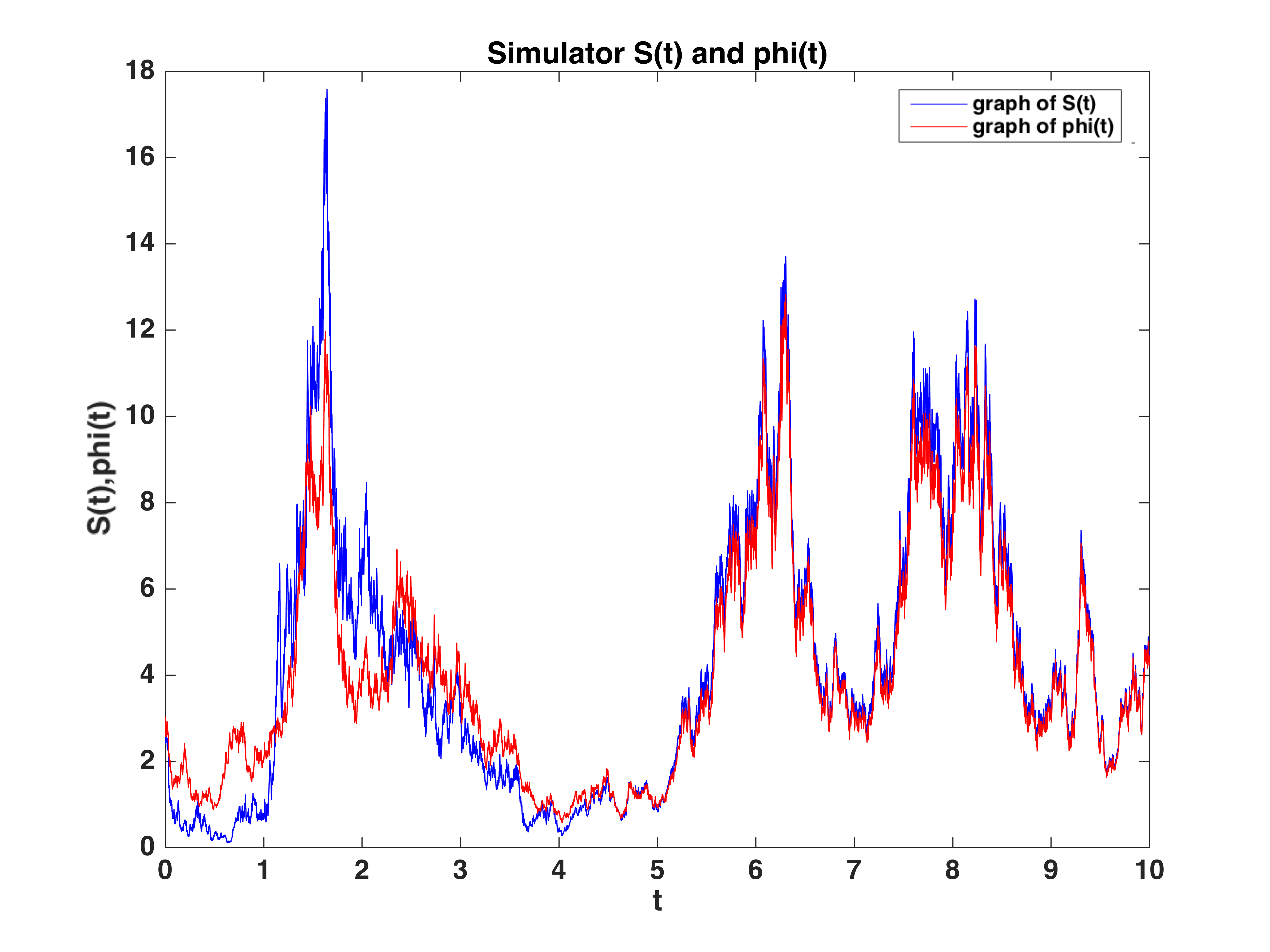
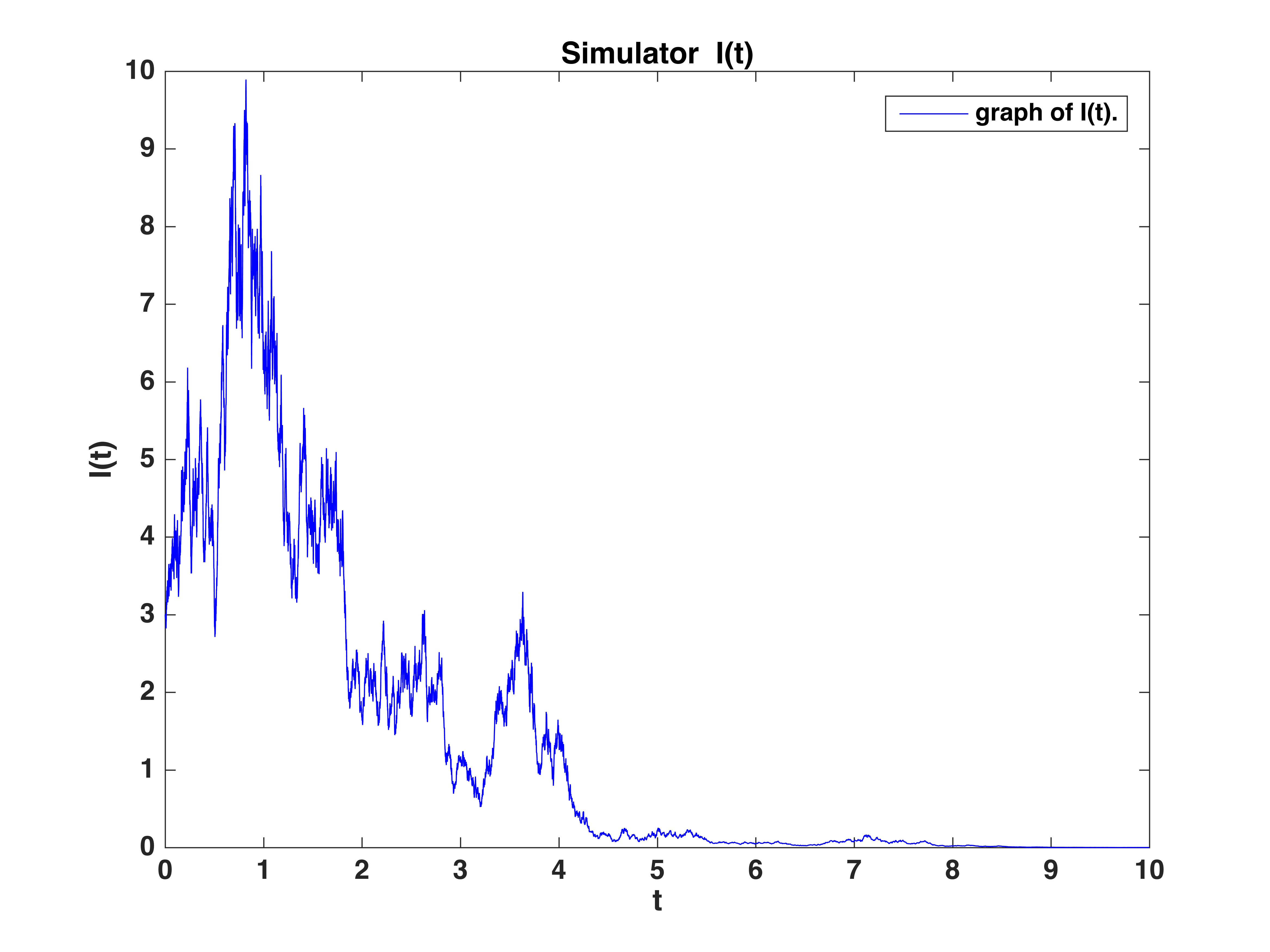
Figure 1: Trajectories of $S(t)$ (blue line) and $\varphi(t)$ (red line) and $I(t)$ in Example 5.1 .

We show an other example where $\lambda>0$ (equivalent $R>1)$.

Example 5.2.

Let $a_{1}=10;b_{1}=1;b_{2}=1;c=6;\sigma_{1}=1;\sigma_{2}=1;m=1.$ Calculating directly obtains $\lambda\approx 3.3611$, which means that the system (5.1) is permanent. Trajectories of $S(t),I(t)$ are shown in Figure 2. Moreover, the system (5.1) has a unique invariant measure $\pi^{*}$ concentrated on $\mathbb{R}_{+}^{2,\circ}$. We draw the empirical density of $\pi^{*}$ and phase portrait $(S(t),I(t))$ in Figure 3.

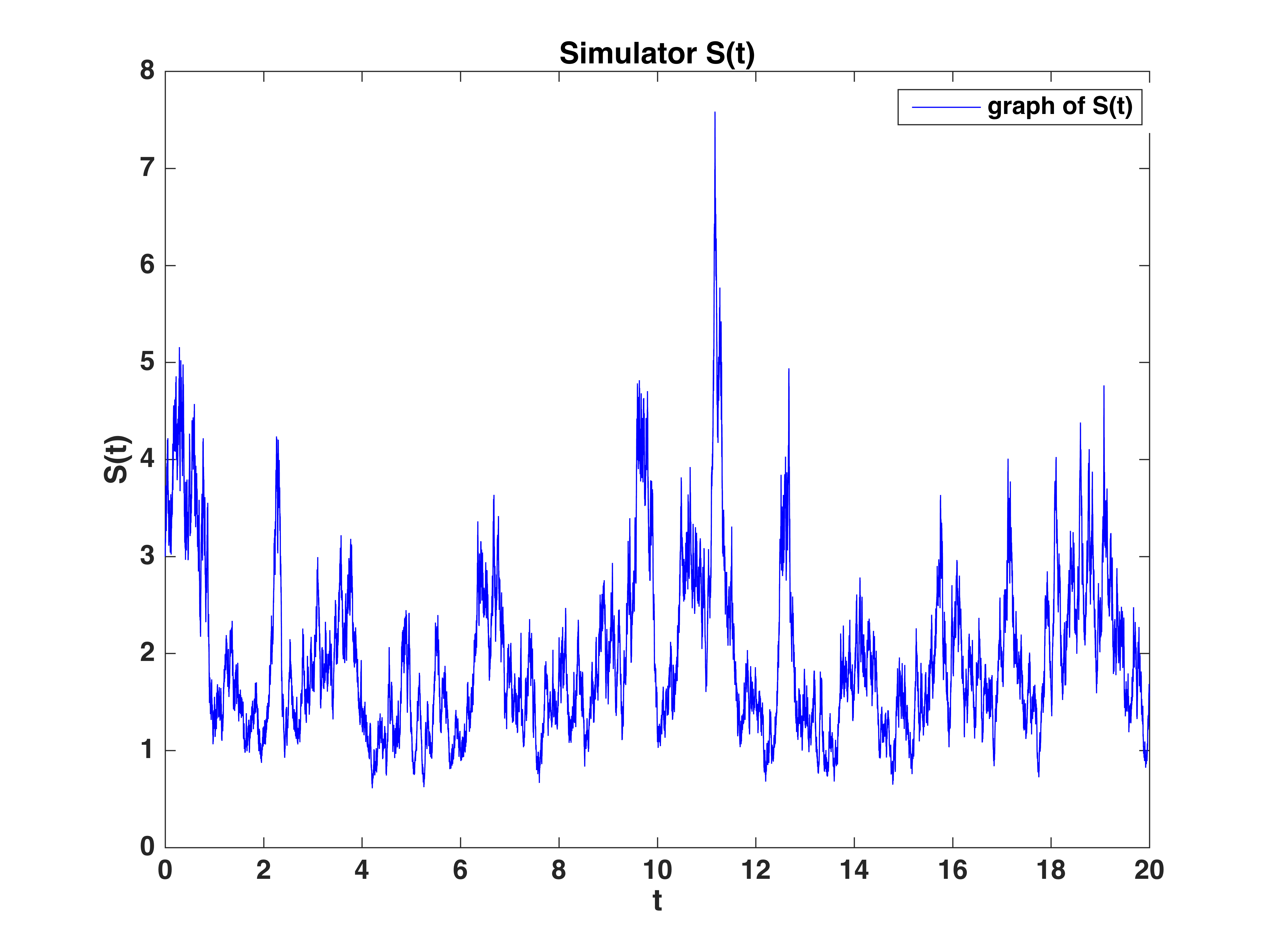
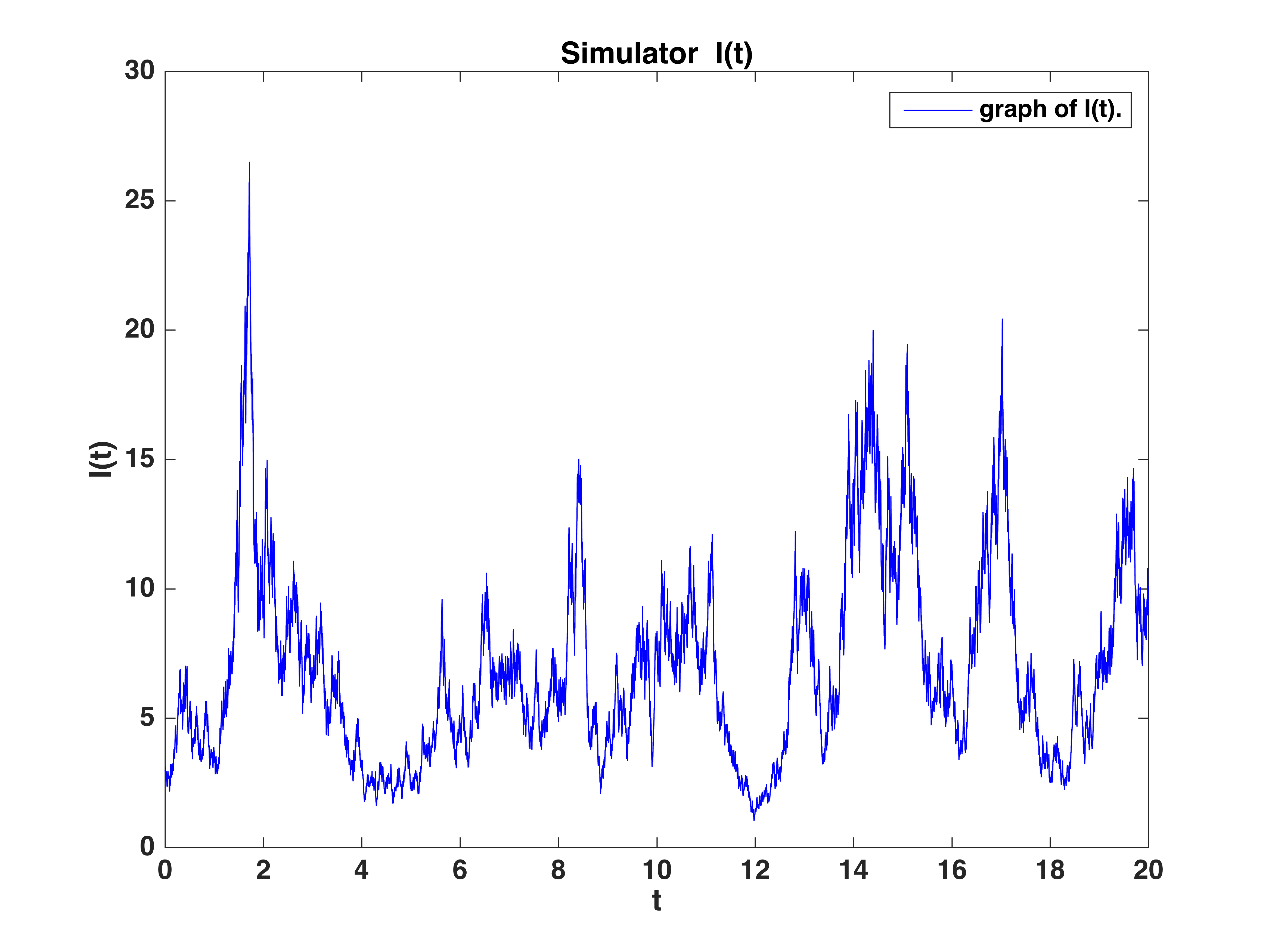
Figure 2: Trajectories of $S(t),I(t)$ in Example 5.2.

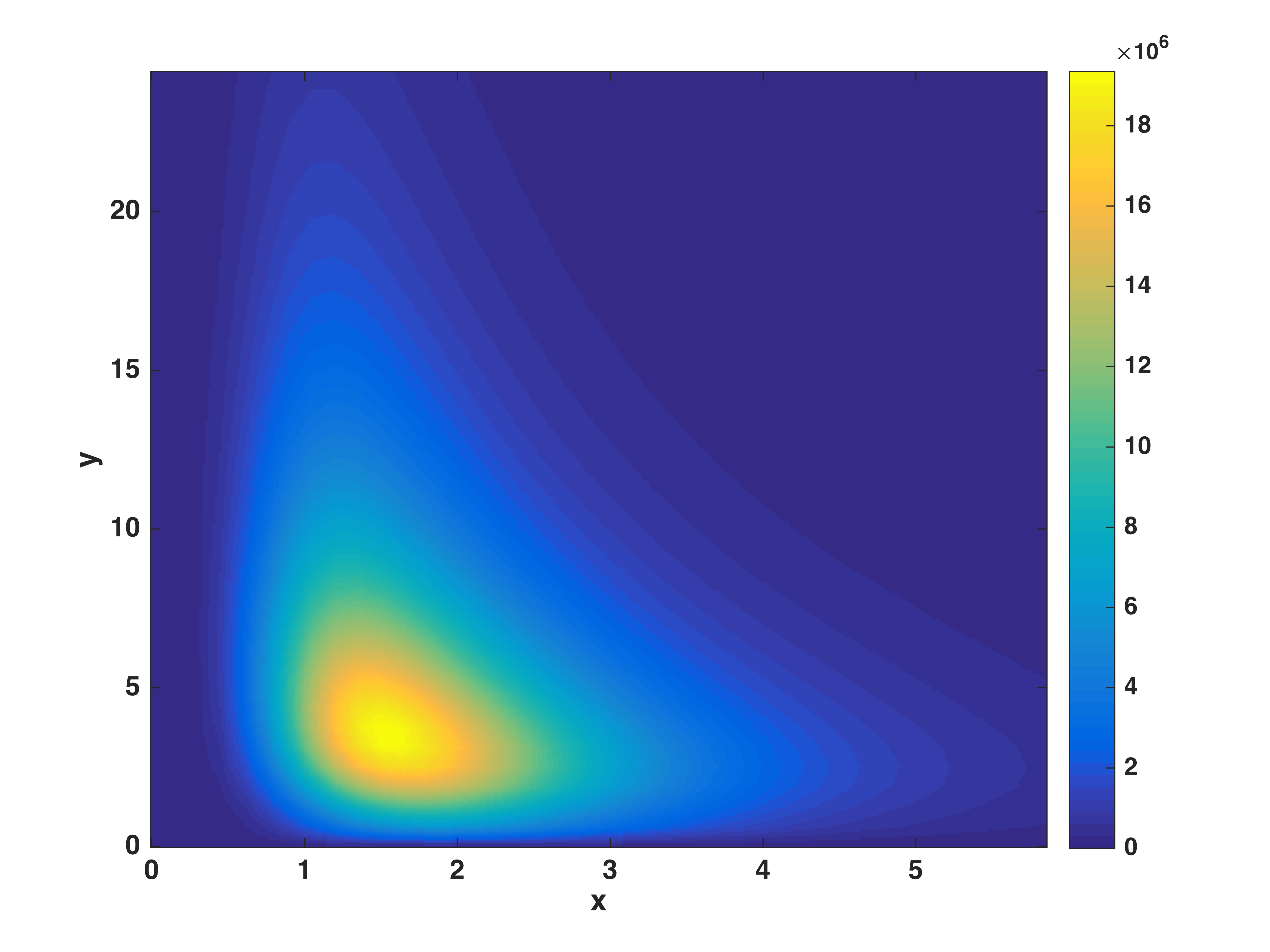
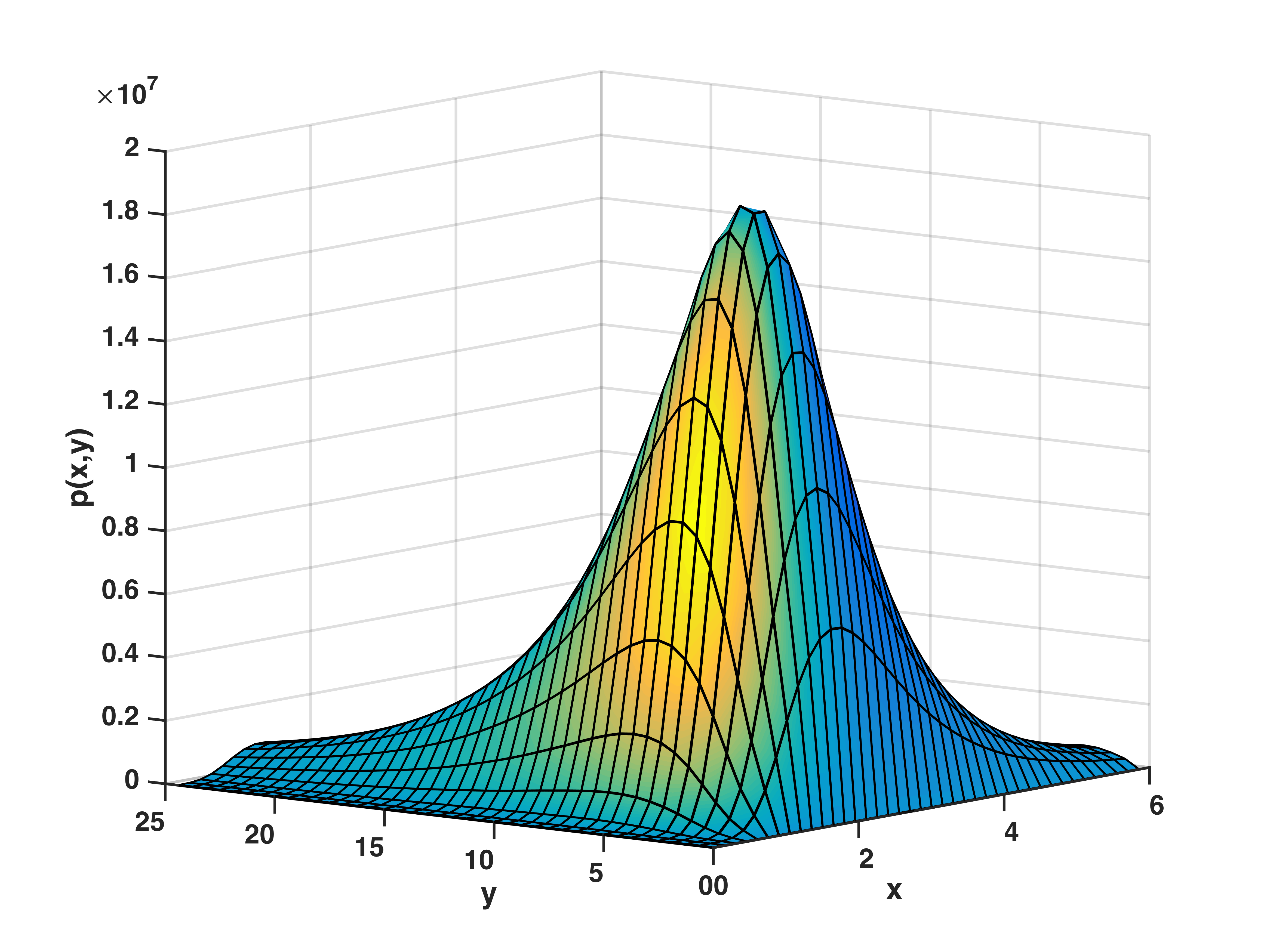
Figure 3: Empirical phase and density of $\pi^{*}$ in Example 5.2 in 2D and 3D settings respectively.

5.2  Discussion

We discuss Theorem 3.1 by providing alternative results in some special cases. In case of $g(s,i)=0$, we can use the comparison Theorem [9, Theorem 1.1, p.437] to obtain that $S_{u,v}(t)\leq\varphi_{u}(t)\text{\;a.s.\;}$ Therefore, we can always dominate $S_{u,v}(t)$ by the ergodic process $\varphi_{u}(t)$ and some estimates can be simplified.

Theorem 5.1.

In case of $g(s,i)=0$, the results in Theorem 3.1 hold without the condition $f(s,0)-\dfrac{1}{2}g^{2}(s,0)$ is monotonic.

Proof.

The proof can be similarly obtained as in [6, proof of Theorem 2.1]. ∎

If the function $\dfrac{F(s,i)}{s}=\dfrac{if(s,i)}{s}$ is uniformly bounded, for example, the Beddington–DeAngelis incidence rate or the nonlinear functional response with $l=h$, we also obtain the results as in Theorem 3.1.

Theorem 5.2.

The results in Theorem 3.1 hold if we replace the condition $f(s,0)-\dfrac{1}{2}g^{2}(s,0)$ is monotonic by the condition $\dfrac{F(s,i)}{s}$ is uniformly bounded.

Proof.

The proof is similar to [5]. ∎

References

- [1] Y. Cai, Y. Kang, M. Banerjee, W. Wang, A stochastic SIRS epidemic model with infectious force under intervention strategies, J. Differential Equations, 259 (2015), 7463–7502.
- [2] R. Cui, K.Y. Lam,Y. Lou, Dynamics and asymptotic profiles of steady states of an epidemic model in advective environments.,J. Differential Equations, 263 (2017), 2343–2373.
- [3] N. H. Dang, G. Yin, Coexistence and Exclusion of Stochastic Competitive Lotka-Volterra Models, J. Differential Equations, 262 (2017), 1192–1225.
- [4] N. T. Dieu, D. H. Nguyen, N. H. Du, G. Yin, Classification of Asymptotic Behavior in A Stochastic SIR Model, SIAM J. Appl. Dyn. Syst., 15 (2016), 1062–1084. 187–202.
- [5] N. H. Du, N. N. Nhu, Permanence and extinction of certain stochastic SIR models perturbed by a complex type of noises, Appl. Math. Lett., 64 (2017), 223–230. .
- [6] N. H. Du, N. T. Dieu, N. N. Nhu, Conditions for Permanence and Ergodicity of Certain SIR Epidemic Models, Acta Appl. Math., 160 (2019), 81–99.
- [7] N. H. Du, N. H. Dang, N. T. Dieu, On stability in distribution of stochastic differential delay equations with Markovian switching, Systems Control Lett., 65 (2014), 43–49.
- [8] L. Huo, J. Jiang, S. Gong, B. He, Dynamical behavior of a rumor transmission model with Holling-type II functional response in emergency event, Phys. A, 450 (2016), 228–240.
- [9] N. Ikeda, S. Watanabe, Stochastic differential equations and diffusion processes, Second edition, North-Holland Publishing Co., Amsterdam, (1989).
- [10] S. F. Jarner, G. O. Roberts, Polynomial convergence rates of Markov chains, Ann. Appl. Prob., 12 (2002), 224–247.
- [11] W. O. Kermack, A. G. McKendrick, Contributions to the mathematical theory of epidemics I, Proc. R. Soc. Lond. Ser. A, 115 (1927), 700–721.
- [12] W. O. Kermack, A. G. McKendrick, Contributions to the mathematical theory of epidemics II, Proc. Roy. Soc. Lond. Ser. A, 138 (1932), 55–83.
- [13] W. Kliemann, Recurrence and invariant measures for degenerate diffusions, Ann. Probab., 15 (1987), 690–707.
- [14] A. Lahrouz, L. Omari, D. Kiouach, Global analysis of a deterministic and stochastic nonlinear SIRS epidemic model, Nonlinear Anal. Model. Control, 16 (2011), 59–76.
- [15] D. Li, S. Liu, J. Cui, Threshold dynamics and ergodicity of an SIRS epidemic model with Markovian switching., J. Differential Equations, 263 (2017), 8873–8915.
- [16] D. Li, S. Liu, J. Cui, Threshold dynamics and ergodicity of an SIRS epidemic model with semi-Markov switching, J. Differential Equations, 266 (2019), 3973-4017.
- [17] X. Mao, Stochastic differential equations and their applications, Horwood Publishing chichester, 1997.
- [18] X. Mao, G. Marion, E. Renshaw, Environmental noise suppresses explosion in population dynamics, Stochastic Process. Appl., 97 (2002), 95–110.
- [19] S. P. Meyn, R. L. Tweedie, Markov Chains and Stochastic Stability, Springer, London, 1993.
- [20] S. P. Meyn, R. L. Tweedie, Stability of markovian processes II: continuous-time processes and sampled chains. Adv. in Appl. Probab., (1993), 487-517.
- [21] D. Nguyen, N. Nguyen, G. Yin, Analysis of a spatially inhomogeneous stochastic partial differential equation epidemic model, to appear in J. Appl. Probab.
- [22] N. Nguyen, G. Yin, Stochastic partial differential equation SIS epidemic models: modeling and analysis, Commun. Stoch. Anal., 13, 8 (2019).
- [23] D. Nguyen, G. Yin, Z. Chu, Certain Properties Related to Well Posedness of Switching Diffusions, Stochastic Process. Appl., 127 (2017), 3135–3158.
- [24] E. Nummelin, General Irreducible Markov Chains and Non-negative Operations, Cambridge Press, (1984).
- [25] S. Ruan, W. Wang, Dynamical behavior of an epidemic model with a nonlinear incidence rate, J. Differential Equations, 188 (2003), 135–163.
- [26] A. V. Skorokhod, Asymptotic Methods in the Theory of Stochastic Differential Equations, Translated from the Russian by H. H. McFaden, Transl. Math. Monogr. 78, American Mathematical Society, Providence, RI, 1989.
- [27] C. Shan, H. Zhu, Bifurcations and complex dynamics of an SIR model with the impact of the number of hospital beds, J. Differential Equations, 257 (2014), 1662–1688.
- [28] C. Shan, Y. Yi, H. Zhu, Nilpotent singularities and dynamics in an SIR type of compartmental model with hospital resources, J. Differential Equations, 260 (2016), 4339–4365.
- [29] Q. Yang, D. Jiang, N. Shi, C. Ji, The ergodicity and extinction of stochastically perturbed SIR and SEIR epidemic models with saturated incidence, J. Math. Anal. Appl., 388 (2012), 248–271.
- [30] C. Zhu, G. Yin, On strong Feller, recurrence, and weak stabilization of regime-switching diffusions, SIAM J. Control Optim., 48 (2009), 2003–2031.
- [31] L. Zhang, Z. C. Wang, X. Q. Zhao, Threshold dynamics of a time periodic reaction–diffusion epidemic model with latent period, J. Differential Equations, 258 (2015), 3011–3036.