The 11 years of low-activity of the magnetar XTE J1810-197

Abstract

In 2003, the magnetar XTE J1810-197 started an outburst that lasted until early 2007. In the following 11 years, the source stayed in a quiescent/low activity phase. XTE J1810-197 is one of the closest magnetars, hence its X-ray properties can be studied in detail even in quiescence and an extended monitoring has been carried out to study its long term timing and spectral evolution. Here, we report the results of new X-ray observations, taken between September 2017 and April 2018, with XMM-Newton, Chandra and NICER. We derived a phase-connected timing solution yielding a frequency derivative of $-9.26(6)\times 10^{-14}$ Hz s^-1. This value is consistent with that measured between 2009 and 2011, indicating that the pulsar spin-down rate remained quite stable during the long quiescent period. A spectral analysis of all the X-ray observations taken between 2009 and 2018 does not reveal significant spectral and/or flux variability. The spectrum of XTE J1810-197 can be described by the sum of two thermal components with temperatures of 0.15 and 0.3 keV, plus a power law component with photon index 0.6. We also found evidence for an absorption line at $\sim$1.2 keV and width of 0.1 keV. Thanks to the long exposure time of the summed XMM-Newton observations, we could also carry out a phase-resolved spectral analysis for this source in quiescence. This showed that the flux modulation can be mainly ascribed to the the warmer of the two thermal components, whose flux varies by $\sim 45$ per cent along the pulse phase.

1 Introduction

Magnetars are isolated neutron stars (NSs) with magnetic fields generally higher than $10^{14}$ G and a X-ray/soft $\gamma$-ray emission believed to be powered by the decay and instability of their extreme internal magnetic fields (e.g. Duncan & Thompson, 1992; Paczynski, 1992; Thompson & Duncan, 2001). They have X-ray luminosities and spin periods in the ranges $L_{X}\sim 10^{31}-10^{36}$ erg s^-1 and $P$$\sim$0.3-12 s, respectively. Most of these sources are strongly variable showing, at unpredictable times, large outbursts during which their X-ray flux increases up to three orders of magnitude and then decays on a variety of timescales (Esposito et al., 2018). Typically, magnetars X-ray spectra are well described by the sum of a thermal component, believed to originate from (a region of) the NS surface, and a power law component, associated to repeated resonant scatterings of the soft thermal photons by relativistic electrons flowing in the magnetosphere. In some cases, additional spectral components are necessary (see e.g. Mereghetti et al., 2009, 2015; Kaspi & Beloborodov, 2017; Turolla et al., 2015; Esposito et al., 2018, for recent reviews).

Although already detected by ROSAT in 1993 as a weak source with a 0.5–10 keV flux of $(5-10)\times 10^{-13}$ erg cm^-2 s^-1, XTE J1810-197 remained unnoticed until it experienced a powerful outburst discovered by RXTE in 2003 (Gotthelf et al. 2004; Ibrahim et al. 2004). Since the initial phases of the outburst were missed, it was possible to set only a lower limit on the peak flux (a factor of 100 higher than the quiescent level). The outburst was followed with a multi-wavelength monitoring, and it was possible to discover X-ray pulsation at $\sim 5.54$ s and to measure a source spin down of $6.7\times 10^{-13}$ s s^-1 (Ibrahim et al., 2004). In addition, several short bursts were seen during the initial phases of the outburst decay (Woods et al., 2005). These properties indicated that XTE J1810-197 could be interpreted as a magnetar. XTE J1810-197 was also the first magnetar detected as a radio pulsar in the radio band (Halpern et al., 2005), where, during the latest phases of the decay, it showed intense and pulsed emission in phase with the X-ray pulsations (Camilo et al. 2006, Camilo et al. 2007; even though it is likely that pulsed radio emission was present also during the initial phases of the outburst). The outburst lasted until early 2007, when the source returned at a flux level similar to that of the pre-outburst epochs (e.g. Alford & Halpern, 2016; Pintore et al., 2016), although its radio emission continued till late 2008 (e.g. Camilo et al., 2016) and a decaying flux from a hot region on the NS surface was present until 2009 (Alford & Halpern, 2016).

Thanks to the continuous monitoring of XTE J1810-197 carried out in the radio and X-ray bands, it was possible to investigate its spin period variability during the outburst decay and in quiescence. The source showed a high and variable spin-down rate during the outburst decay (between $-1\times 10^{-13}$ and $-5\times 10^{-13}$ Hz s^-1) and a more stable spin-down rate during the quiescent phase ($\sim-9.2\times 10^{-14}$ Hz s^-1; Pintore et al. 2016; Camilo et al. 2016).

The spectral properties of XTE J1810-197 during the outburst decay could be well modelled by the sum of three blackbody components with temperatures of $\sim 0.15$, 0.3 and 0.7 keV. They were associated to the whole NS surface and to two concentric hot-spots on the NS surface (Bernardini et al., 2009; Albano et al., 2010; Alford & Halpern, 2016; Pintore et al., 2016; Coti Zelati et al., 2018). During the quiescent phase following the outburst, the spectrum could be fit with only two blackbody components (e.g. Bernardini et al., 2009). Note that the quiescent spectrum seen with ROSAT before the 2003 outburst could be fit with a single blackbody, but this might be due to the limited bandwith and counting statistics of the data (e.g. Bernardini et al., 2009).

Here we first report the spectral and timing analysis of a new set of XMM-Newton, Chandra and NICER observations taken between June 2017 and April 2018 and then we use the whole dataset of the long quiescent period (2007–2018) to carry out a sensitive spectral analysis.

2 Data Reduction

2.1 XMM-Newton

Table 1: Log of the XMM-Newton, Chandra and NICER observations.

Obs.	Telescope	Obs. ID	Epocha	Duration
No.			MJD	ks
1	XMM-Newton	0552800201	54895.6543341	63.6
2	XMM-Newton	0605990201	55079.6256771	19.4
3	XMM-Newton	0605990301	55081.5548494	17.7
4	XMM-Newton	0605990401	55097.7062563	12.0
5	XMM-Newton	0605990501	55295.1863453	7.7
6	XMM-Newton	0605990601	55444.6796630	9.1
7	XMM-Newton	0671060101	55654.0878884	17.4
8	XMM-Newton	0671060201	55813.3872852	13.7
9	XMM-Newton	0691070301	56176.9826811	15.7
10	XMM-Newton	0691070401	56354.1968379	15.7
11	XMM-Newton	0720780201	56540.8584298	21.2
12	XMM-Newton	0720780301	56720.9705351	22.7
13	NICER	0020420104	57929.3250089	0.8
14	NICER	0020420105	57930.0893007	0.4
15	NICER	0020420106∗	57932.3480273	2.7
16	NICER	0020420107	57934.9969029	0.2
17	NICER	0020420108∗	57938.0619294	2.1
18	NICER	0020420109∗	57939.3048476	1.0
19	NICER	0020420111∗	57947.2165493	3.0
20	NICER	0020420112	57948.1692505	0.7
21	NICER	1020420102∗	57975.1431786	1.3
22	NICER	1020420103	57976.3637636	0.9
23	NICER	1020420104∗	57980.7382669	0.8
24	NICER	1020420105	57981.0546200	0.5
25	NICER	1020420106	57982.0847836	2.2
26	NICER	1020420107	57983.1132332	1.3
27	NICER	1020420108∗	57984.4005154	1.0
28	NICER	1020420109∗	57985.3003735	0.8
29	NICER	1020420110	57987.3589781	0.3
30	NICER	1020420111	57988.1462045	0.5
31	NICER	1020420112∗	57990.1375294	1.6
32	NICER	1020420113∗	57991.3490457	1.8
33	NICER	1020420114∗	57992.3801485	3.0
34	NICER	1020420115∗	57993.1526852	1.6
35	XMM-Newton	0804590201	58002.0363052	16.5
36	XMM-Newton	0804590301	58003.0716635	11.2
37	XMM-Newton	0804590401	58005.9931466	16.6
38	XMM-Newton	0804590501	58011.8023528	10.7
39	XMM-Newton	0804590601	58019.9415131	20.7
40	NICER	1020420116	58055.2523809	0.6
41	NICER	1020420117	58056.4744915	1.3
42	Chandra	20091	58059.3379341	22.6
43	NICER	1020420119	58061.0605071	0.6
44	NICER	1020420121∗	58063.1811345	2.0
45	NICER	1020420122	58158.9468048	0.3
46	NICER	1020420123	58163.1145907	0.4
47	NICER	1020420124	58164.4848159	1.0
48	NICER	1020420125	58165.1774763	0.7
49	NICER	1020420126∗	58166.0236104	1.1
50	XMM-Newton	0804590701	58180.8521837	10.4
51	NICER	1020420127	58213.6570253	0.5

^a Mean time of the observation. ^∗ NICER observations where source pulsation was detected.

We analyzed 18 XMM-Newton observations taken between March 2009 and March 2018 (see Table 1; the 2017–2018 observations are reported here for the first time). For each observation, we reduced the data of the EPIC-pn and the two EPIC-MOS cameras using sas v.16.1.0. We excluded the pixels at the CCD edges (FLAG=0), selected single- and double-pixel events (i.e. pattern$\leq$4) and single- and multiple-pixel events (i.e. pattern$\leq$12) for pn and MOS, respectively. We extracted source and background counts from circular regions of radii of 35^′′ and 60^′′, respectively. For the spectral analysis, we filtered the data excluding time intervals with high background and we rebinned the spectra to have at least 100 counts per bin.

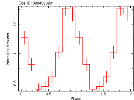
Figure 1: Pulse profile of XTE J1810-197 in the 1-6 keV range obtained in the XMM-Newton observation 0804590201. The pulse profiles of all the other 2017-2018 observations are very similar. They can be well described by a single sinusoid with average pulsed fraction of $\sim 30$ per cent.

We corrected the source photons times of arrival to the solar system barycenter adopting the source most accurate coordinates R.A. = 18^h 09^m 51.09^s, Dec. = –19^∘ 43^′ 51.9^′′ (Camilo et al., 2006). No source bursts were detected during any of the observations reported here. Comparison of the pn and MOS data showed that the XMM-Newton observation Obs.ID=0804590401 was affected by an instrumental problem which causes the shift of 1 second in the event times of the pn detector (the MOS is not affected by this issue, see e.g. Martin-Carrillo et al. 2012 ). We corrected this problem by adding a second to the pn event times.

The RGS data of all observations were reduced following the standard procedure. For each dataset, we extracted the source spectra and grouped them with at least 30 counts per bin.

2.2 Chandra

We analyzed a Chandra ACIS-S observation taken on 2017 November 2, with an exposure time of $\sim 20$ ks (see Table 1). We used ciao v.4.9 and calibration files CALDB v.4.7.6. to perform the data reduction. We extracted source and background events from circular regions of radii of 3^′′ and 15^′′, respectively, and we barycentered the data with the task axbary. Also in this case, no source bursts were found. The source spectra were produced with the task specextract, which generates the corresponding response and auxiliary files for the spectral analysis. Spectra were rebinned with at least 25 counts per bin.

2.3 NICER

We analyzed all the available NICER (e.g. Gendreau et al., 2012) observations taken between June 2017 and April 2018 (see Table 1). We extracted the data with nicerdas version 2018-02-22 (v2d) and adopting the tool nicerl2. We then barycentered the data with the barycorr task. These datasets were used only for the timing analysis because of the lack of imaging capabilities, which precludes the extraction of a properly background-subtracted spectrum for XTE J1810-197.

3 Results

3.1 Timing

Analysis of the source spin frequency based on XMM-Newton and Chandra observations between 2003 and 2014 has been already reported in Bernardini et al. (2009), Alford & Halpern (2016), Pintore et al. (2016) and Camilo et al. (2016). Therefore, we analyzed only the 2017-2018 NICER, Chandra and XMM-Newton observations, performing a Z² search around the expected spin frequency. We selected the energy range 1–6 keV, which yields the highest signal-to-noise ratio. The source pulsations were significantly detected in all XMM-Newton and Chandra observations, while only a subset of the NICER observations (shown in Table 1) had high-enough counting statistics to allow the pulse detection. The average spin frequency in the whole 2017–2018 dataset is $0.180461(1)$ Hz. The pulse profile can be modelled by a single sinusoidal component with average pulsed fraction of $28\pm 2$ per cent (Figure 1).

To determine the spin period evolution, we initially phase-connected the pulse phases of the NICER observations between 25-28 August 2017 (observations #31–#34), separated in time by $\sim$1d (see Table 1). We fitted the pulse phases with a linear function of the form $\phi(t)=\phi_{0}+\nu_{0}(t-T_{0})$, where $\nu_{0}$ is the spin frequency at the reference epoch $T_{0}$ (MJD 58002.5 in our analysis). Then, we added one by one all the other observations that could be phase-connected. After $\sim$30 days, a quadratic term of the form $\dot{\nu}(t-T_{0})^{2}/2$ started to be statistically significant. Finally, we connected all the observations from June 2017 to April 2018, finding a timing solution with $\nu_{0}=0.180461427(4)$ Hz and $\dot{\nu}=-9.26(6)\times 10^{-14}$ Hz s^-1 (see Figure 2 and Table 2). A second frequency derivative was not statistically required for this dataset. The timing solution cannot be extended to the XMM-Newton observations obtained before 2014 because of the uncertainties on the timing parameters.

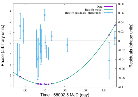
Figure 2: Timing solution of the 2017-2018 NICER, Chandra and XMM-Newton observations (purple points). Cyan points are the residuals in phase-units of the best-fit solution (green line) with $\nu_{0}=0.180461427$ Hz and $\dot{\nu}=-9.26\times 10^{-14}$ Hz s^-1, for T${}_{0}=58002.5$ MJD.

Table 2: Best-fit timing solution of the XMM-Newton, NICER and Chandra observations. Errors are at 1$\sigma$ and estimated after adding a systematic uncertainty to the time of arrivals in order to obtain a reduced $\chi^{2}$ of 1.

Parameter	Value	Units
Time range	57932–58181	MJD
$T_{0}$	58002.5	MJD
$\nu_{0}$	0.180461427(4)	Hz
$\dot{\nu}$	$-9.26(6)\times 10^{-14}$	Hz s-1
$P_{0}$	5.5413504(1)	s
$\dot{P}$	$2.84(2)\times 10^{-12}$	s s-1
$\chi_{\nu}^{2}(dof)$	2.37(16)

3.2 Spectral analysis

We performed a spectral analysis on all the XMM-Newton and the 2017 Chandra observations, using xspec v.12.10.0 (Arnaud, 1996), fitting the spectra in the 0.3–10 keV energy range. Interstellar absorption was included using the tbabs model with the solar abundances of Wilms et al. (2000). All the errors on the spectral parameters are at 90 per cent confidence level.

We checked that there were no significant differences in source flux or spectral shape in the 2017 and 2018 observations and that they were consistent, within the uncertainties, with those of all the previous XMM-Newton observations during quiescence (i.e. observation from $\#1$ to $\#12$). Therefore, we were allowed to stack all the EPIC-pn, EPIC-MOS and RGS data into single spectra.

The stacked EPIC-MOS and pn spectra were then fitted simultaneously. No good fits could be obtained with either a single ($\chi^{2}$/dof=3646.35/879) or the sum of two blackbody components ($\chi^{2}$/dof=1149.86/877; Figure 3-central panel). We obtained an acceptable fit ($\chi^{2}$/dof=897.62/872) by adding to the two-blackbody model a power law with photon index $\Gamma\sim 0.6$ and an absorption line at $\sim 1.2$ keV. The latter was modeled with a Gaussian profile (gabs in xspec). The best fit spectrum is shown in Figure 3 and all the corresponding parameters are reported in Table 3. The column density of $\sim 1.15\times 10^{22}$ cm^-2 is close to that reported in Alford & Halpern (2016) and Coti Zelati et al. (2018). The blackbody components have temperatures of kT${}_{1}\sim 0.15$ keV and kT${}_{2}\sim 0.3$.

We note that the power-law can be replaced with a third blackbody component, which provides a statistically acceptable fit as well ($\chi^{2}$/dof=897.1/872), although with poorly constrained parameters (kT = $2.5_{-0.9}^{+2.7}$ keV and emitting radius of $3_{-1.6}^{+2.9}$ meters). Such a hot blackbody was never observed in this source even during the outburst decay. In fact, the third blackbody component used to model the source spectra (e.g. Bernardini et al., 2009) had at significantly lower temperatures ($\sim 0.5-0.7$ keV). For this reason, in the following we consider only the powerlaw option.

We estimated that the average absorbed 0.3–10 keV flux is $(8.04\pm 0.07)\times 10^{-13}$ erg cm^-2 s^-1, which is very close to the quiescent value reported in Pintore et al. (2016), Camilo et al. (2016) and Coti Zelati et al. (2018), and close to the pre-outburst quiescent flux ($(5-10)\times 10^{-13}$ erg cm^-2 s^-1; Gotthelf et al. 2004; Gotthelf & Halpern 2007). For a distance of $3.5\pm 0.05$ kpc (Minter et al., 2008), the fluxes of the blackbody components imply emitting regions with radii of $1.18_{-0.18}^{+0.20}$ km and $21.3_{-3.2}^{+3.4}$ km for the warmer and colder components, respectively. The blackbody components carry $\sim 64$ and $\sim 33$ per cent of the total flux for the warmer and colder component, respectively, while the powerlaw/blackbody component only $\sim 3$ per cent.

To check whether the line at 1.2 keV in the EPIC spectrum could be due to a blend of narrow lines, we examined the RGS spectrum. This was fitted with the same continuum model (2 blackbodies + powerlaw) used for EPIC and did not show the presence of statistically significant narrow lines around 1.2 keV (see Figure 4).

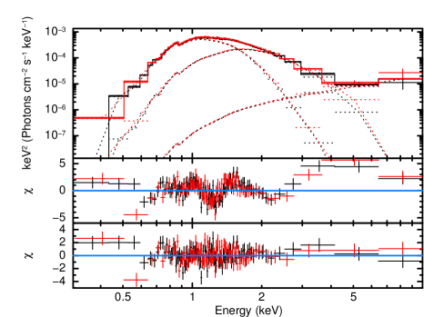
Figure 3: Top panel: Stacked EPIC-pn (black) and MOS (red) spectra of all the XMM-Newton observations. The solid line is the best fit model (tbabs*gabs*(bbodyrad + bbodyrad + powerlaw) in XSPEC). The best-fit residuals are shown in the bottom panel. The middle panel shows the residuals obtained without the Gaussian line and power-law components. Data have been rebinned for display purpose only.

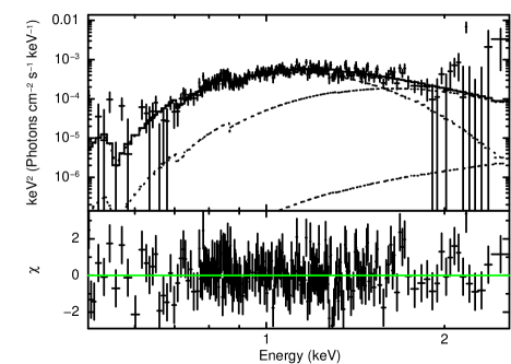
Figure 4: Combined RGS spectrum of XTE J1810-197  fitted with the best-fit (continuum model only) found for the EPIC-pn and MOS spectra. A weak, narrow absorption feature is seen at $\sim 1.3$ keV although not statistically significant.

Table 3: Best-fit of the stacked EPIC-pn and EPIC-MOS spectra with the tbabs*gabs(bbodyrad + bbodyrad + powerlaw) model. Errors are at 90 per cent for each parameter of interest.

Model	Component
TBabs	nH ($10^{22}$)	$1.16^{+0.03}_{-0.03}$
bbodyrad	kT1 (keV)	$0.143^{+0.004}_{-0.004}$
	Norm. ($10^{3}$)	$3.7^{+1.0}_{-0.7}$
bbodyrad	kT2 (keV)	$0.30^{+0.01}_{-0.01}$
	Norm.	$11.4^{+4.0}_{-2.8}$
powerlaw	$\Gamma$	$0.6^{+1.1}_{-0.9}$
	Norm. (10-7)	$8.9^{+43}_{-7.0}$
gabs	Energy (keV)	$1.24^{+0.01}_{-0.01}$
	$\sigma$ (keV)	$0.1^{+0.02}_{-0.02}$
	Strength (keV)	$0.035^{+0.01}_{-0.008}$
$\chi^{2}_{\nu}(dof)$		1.03(872)

3.2.1 Phase-resolved spectroscopy

We extracted EPIC-pn spectra for seven phase bins (see Figure 5) and fitted them simultaneously using the best-fit model of the phase-averaged spectrum with parameters fixed to those of Table 3, with the addition of a multiplicative factor to account for the different flux in each phase bin. This is clearly a poor reproduction of the spectra ($\chi^{2}$/dof=1370.15/197), indicating the presence of spectral variability along the pulse-profile. Therefore, we removed the multiplicative constant and we let the normalizations of the blackbody components free to vary independently: in this way we could properly fit the data ($\chi^{2}$/dof=221.51/189). The normalizations of the two blackbodies followed very well the shape of the pulse profile. The variability is larger for the warmer blackbody, for which the normalization varies by $\sim 45$ per cent, compared to $\sim 10$ per cent for the colder one. In Figure 5, we present the emitting radius of the two blackbodies as a function of the spin-phase, for a distance of 3.5 kpc, showing a pulsed fraction of $\sim 26$ and $\sim 6$ per cent. We also tried to let free to vary independently (one parameter at the time), the blackbody temperatures, the powerlaw normalization and the line normalization. The fit was generally poorly sensitive to these parameters, but we found some hint for an anti-correlation between the line intensity and the total flux. To test further the line behaviour, we extracted only two EPIC-pn spectra for the phase bins 0.75–1.2 (the minimum of the pulse profile) and 0.2–0.75 (the pulse peak) and we fitted them with the average best-fit model letting free to vary only the blackbodies and line normalization ($\chi^{2}$/dof=221.54/185). This analysis indicated that the line optical depth changes from $0.050\pm 0.007$ at the pulse peak to $0.032\pm 0.005$ at the pulse minimum, implying a measured variability at the $\sim$2$\sigma$ level.

4 Discussion

XTE J1810-197 was one of the first transient magnetar to be discovered and it is the one for which it has been possible to observe the longest quiescent period following an outburst ($\sim 11$ years). In fact, other transient magnetars, such as, e.g., 1E 1547.0–5408 and SGR 1627–41, displayed shorter quiescent periods, interrupted by the occurrence of recurrent outbursts (see e.g. Coti Zelati et al., 2018). In addition, since XTE J1810-197 is relatively close (3.5 kpc, Minter et al. 2008), its quiescent luminosity of $\sim 10^{33}$ erg s^-1 yields a flux sufficiently high to permit sensitive spectral and timing studies.

After the decay of its outburst in early 2007, XTE J1810-197 entered a low-activity phase during which the source pulsation could be still significantly detected. The quality of the timing data during this phase was good enough to measure precisely the spin-down ($\dot{\nu}\sim-9.2\times 10^{-14}$ Hz s^-1) and to find evidence of a second derivative term ($\ddot{\nu}\sim 5.7\times 10^{-23}$ Hz s^-2). This phase-connected timing solution was found to be valid for a baseline of $\sim 1000$d (between 2009 and 2011), but strong timing noise made it impossible to extend it to earlier or later epochs (e.g. Pintore et al., 2016; Camilo et al., 2016). Assuming that this timing solution remained valid until the time of the observations reported here, we would expect a spin frequency of 0.18046226(15) Hz in the first 2017 XMM-Newton observation. This is indeed quite close to the average frequency measured in the 2017–2018 monitoring (0.180461(1) Hz). Thanks to the new XMM-Newton, Chandra observations and the dense NICER monitoring, we could derive a new phase-connected timing solution characterized by a source spin-down of $-9.26(6)\times 10^{-14}$ Hz s^-1, which is totally consistent within uncertainties with that reported for the years 2009-2011. No significant second derivative component was observed and we derived 2$\sigma$ limits of $-2\times 10^{-22}$ Hz s^-2 $<\ddot{\nu}<1\times 10^{-21}$ Hz s^-2, which are consistent with previous estimates (e.g. Camilo et al., 2016). Further X-ray observations in 2019 could allow us to obtain a more precise timing solution, which could also be extended backwards in time. We note that our timing solution does not exhibit strong timing noise during the $\sim 8$ months of observations.

Figure 5: Emitting radius of the warmer (top) and colder (bottom) blackbodies along the pulse profile. Errors are at 90 per cent.

The spectral analysis of the new XMM-Newton and Chandra datasets shows that XTE J1810-197 spectrum did not change significantly during its long quiescent phase. It comprises two thermal components with temperatures of $\sim$0.15 keV and 0.3 keV, with associated emission radii of $\sim$ 21 km and 1.1 km (assuming a distance of 3.5 kpc) plus a powerlaw. Such a spectral decomposition for XTE J1810-197 was adopted in Gotthelf et al. (2004), Bernardini et al. (2009), Alford & Halpern (2016), Coti Zelati et al. (2018). While the warmer component has an emitting radius consistent with a hot, localized spot on the NS surface, the large radius associated to the cooler blackbody is of the order of the whole NS size, or even larger. This could be due to the uncertainty in the distance or to the fact that we used simple blackbody models. We note that the currently available neutron star atmosphere models generally yield higher temperature and smaller radii than blackbody fits. It should therefore be explored if more physical spectral models, adequate for the magnetars, could give more realistic values for the emitting radius (e.g. Zavlin & Pavlov, 2004; Potekhin, 2014). If the warmer component originated by a localized heating of the surface layers during the outburst, because of either Ohmic dissipation of back flowing currents in a twisted magnetosphere (Beloborodov, 2009) or energy release in the crust (Pons & Rea, 2012), a substantial decrease of the temperature is to be expected in a timescale of $\sim$1 year. However, in our results, the warmer component appears to be quite stable over the last 11 years and, if this is indeed a hot-spot onto the NS surface, a continuous injection of energy, possibly coming for the star interior, seems to be required (e.g. Kaminker et al., 2014; Akgün et al., 2018). We also found evidence for a hard component that we modelled either with a powerlaw or a blackbody, which is yet not robustly constrained in both cases. We note that hints of an excess at high energy was already seen in the XMM-Newton spectra presented in Bernardini et al. (2009). We exclude the possibility that the component has thermal origin, as it would be too hot, associated to a tiny region on the surface and, especially, it was never observed in the past. On the other hand, the powerlaw model is more reliable and such a component would be associated to resonant scattering of thermal photons from particles flowing in the star magnetosphere (Thompson et al. 2002; see also Turolla et al. 2015 for a review). Further investigations are required to constrain better the nature of such component.

Taking advantage of the large amount of X-ray data and the apparent absence of spectral variability, we also performed for the first time a phase-resolved spectral analysis of the quiescent epochs monitored with XMM-Newton. We found that the radius of the emitting region of the warmer component varies as a function on the pulse-phase with an amplitude of $\sim 26$ per cent (between 0.8–1.5 km), while spectral fits do not indicate variations of the temperature with phase. This finding corroborates the association of this component with a hot-spot, seen with a changing apparent emitting radius caused by the pulsar rotation. However, we found that also the lower temperature component exhibits a change in the emitting radius, although less prominent ($\sim 6$ per cent). Under the assumption that thermal photons come from the star surface, the fractional variation of the emitting areas depends on their size and location, as well as on the angle $\xi$ that the line-of-sight makes with the star rotation axis. Following the approach of Turolla & Nobili (2013), we calculated the relative change of the visible emitting areas over a rotational period using a simple emission model in which the warmer blackbody is emitted by a circular hot-spot with aperture 5° at colatitude $\chi$ (the angle between the rotation axis and the magnetic field axis) and the colder component by a larger, concentric corona. The choice of considering concentric regions is motivated by the fact that the two pulsed components are aligned in phase. Each region is assumed to be at constant temperature. The computation includes general-relativistic effects ($M=1.4M_{\odot}$, $R=10$ km) and was performed for several values of $\chi$ and $\xi$ in the range $[0,\,\pi/2]$. The main conclusion is that there are indeed geometries for which the observed values of the fractional variation are recovered, but this occurs only if the colder region extends over a very large fraction of the star surface. A possible configuration reproducing the observed pulsed fractions is obtained for $\chi\sim 75$°, $\xi\sim 15$° and an aperture of 115° for the colder region. This is of course an oversimplified model. It is likely that the colder blackbody component actually originates from the whole NS with a non-uniform temperature distribution across the surface, that cannot be resolved into more than one thermal component due to the limited sensitivity of the current data.

We also found evidence in the phase-averaged spectrum of an absorption line centered at $\sim 1.25$ keV and with a width of $\sim 0.1$ keV. This feature was already reported in Bernardini et al. (2009), Alford & Halpern (2016), Coti Zelati et al. (2018), and possibly with an asymmetrical shape (Vurgun et al., 2018), and tentatively associated to a resonant cyclotron scattering absorption line. If the line is due to cyclotron scattering/absorption by electrons, the implied magnetic field is $B=10^{12}(E_{c}/11.6\,{\mathrm{k}eV}(1+z))\ \mathrm{G}$ which, assuming $z=0.8$, yields in the present case $B\sim 2\times 10^{11}\ \mathrm{G}$. This is much below the value of the B-field estimated from spin-down. On the other hand, assuming that the line is due to proton cyclotron gives a value $m_{p}/m_{e}$ times higher, $B\sim 3.5\times 10^{14}\,\mathrm{G}$ quite close to that inferred from timing, $B_{p}\sim 2.6\times 10^{14}\,\mathrm{G}$ (e.g. Camilo et al., 2016).

The phase-resolved spectral analysis indicates that the line optical depth may show an anti-correlation with the pulse-profile, the optical depth being lower at the pulse peak and larger near the pulse minimum. As no interstellar absorption line would behave in such a way, this is a further robust support to the intrinsic source origin of such a feature. In addition, this result prompts us to suggest that the line is formed in a region located above the NS surface but that is somehow displaced from the region where the pulse is produced (otherwise the optical depth of the line during the peak should show a maximum).

References

- Akgün et al. (2018) Akgün T., Cerdá-Durán P., Miralles J. A., Pons J. A., 2018, MNRAS, 474, 625
- Albano et al. (2010) Albano A., Turolla R., Israel G. L., Zane S., Nobili L., Stella L., 2010, ApJ, 722, 788
- Alford & Halpern (2016) Alford J. A. J., Halpern J. P., 2016, ApJ, 818, 122
- Arnaud (1996) Arnaud K. A., 1996, in Jacoby, G. H. and Barnes, J., eds., Astronomical Data Analysis Software and Systems V. Vol. 101 of ASP Conf. Ser., San Francisco CA, XSPEC: The First Ten Years. p. 17
- Beloborodov (2009) Beloborodov A. M., 2009, ApJ, 703, 1044
- Bernardini et al. (2009) Bernardini F., et al., 2009, A&A, 498, 195
- Bernardini et al. (2009) Bernardini F., Israel G. L., Dall’Osso S., Stella L., Rea N., Zane S., Turolla R., Perna R., Falanga M., Campana S., Götz D., Mereghetti S., Tiengo A., 2009, A&A, 498, 195
- Camilo et al. (2016) Camilo F., Ransom S. M., Halpern J. P., Alford J. A. J., Cognard I., Reynolds J. E., Johnston S., Sarkissian J., van Straten W., 2016, ApJ, 820, 110
- Camilo et al. (2007) Camilo F., Ransom S. M., Halpern J. P., Reynolds J., 2007, ApJ, 666, L93
- Camilo et al. (2006) Camilo F., Ransom S. M., Halpern J. P., Reynolds J., Helfand D. J., Zimmerman N., Sarkissian J., 2006, Nature, 442, 892
- Coti Zelati et al. (2018) Coti Zelati F., Rea N., Pons J. A., Campana S., Esposito P., 2018, MNRAS, 474, 961
- Duncan & Thompson (1992) Duncan R. C., Thompson C., 1992, ApJ, 392, L9
- Esposito et al. (2018) Esposito P., Rea N., Israel G. L., 2018, ArXiv e-prints
- Gendreau et al. (2012) Gendreau K. C., Arzoumanian Z., Okajima T., 2012, in Space Telescopes and Instrumentation 2012: Ultraviolet to Gamma Ray Vol. 8443 of Proc. SPIE, The Neutron star Interior Composition ExploreR (NICER): an Explorer mission of opportunity for soft x-ray timing spectroscopy. p. 844313
- Gotthelf & Halpern (2007) Gotthelf E. V., Halpern J. P., 2007, ApJ, 664, L35
- Gotthelf et al. (2004) Gotthelf E. V., Halpern J. P., Buxton M., Bailyn C., 2004, ApJ, 605, 368
- Halpern et al. (2005) Halpern J. P., Gotthelf E. V., Becker R. H., Helfand D. J., White R. L., 2005, ApJ, 632, L29
- Ibrahim et al. (2004) Ibrahim A. I., Markwardt C. B., Swank J. H., Ransom S., Roberts M., Kaspi V., Woods P. M., Safi-Harb S., Balman S., Parke W. C., Kouveliotou C., Hurley K., Cline T., 2004, ApJ, 609, L21
- Kaminker et al. (2014) Kaminker A. D., Kaurov A. A., Potekhin A. Y., Yakovlev D. G., 2014, MNRAS, 442, 3484
- Kaspi & Beloborodov (2017) Kaspi V. M., Beloborodov A. M., 2017, ARA&A, 55, 261
- Martin-Carrillo et al. (2012) Martin-Carrillo A., Kirsch M. G. F., Caballero I., Freyberg M. J., Ibarra A., Kendziorra E., Lammers et al. 2012, A&A, 545, A126
- Mereghetti et al. (2009) Mereghetti S., Götz D., Weidenspointner G., von Kienlin A., Esposito P., Tiengo A., Vianello G., Israel G. L., Stella L., Turolla R., Rea N., Zane S., 2009, ApJ, 696, L74
- Mereghetti et al. (2015) Mereghetti S., Pons J. A., Melatos A., 2015, Space Sci. Rev., 191, 315
- Minter et al. (2008) Minter A. H., Camilo F., Ransom S. M., Halpern J. P., Zimmerman N., 2008, ApJ, 676, 1189
- Paczynski (1992) Paczynski B., 1992, Acta Astronomica, 42, 145
- Pintore et al. (2016) Pintore F., Bernardini F., Mereghetti S., Esposito P., Turolla R., Rea N., Coti Zelati F., Israel G. L., Tiengo A., Zane S., 2016, MNRAS, 458, 2088
- Pons & Rea (2012) Pons J. A., Rea N., 2012, ApJ, in press (astro-ph/1203.4506)
- Potekhin (2014) Potekhin A. Y., 2014, Physics Uspekhi, 57, 735
- Thompson & Duncan (2001) Thompson C., Duncan R. C., 2001, ApJ, 561, 980
- Thompson et al. (2002) Thompson C., Lyutikov M., Kulkarni S. R., 2002, ApJ, 574, 332
- Turolla & Nobili (2013) Turolla R., Nobili L., 2013, ApJ, 768, 147
- Turolla et al. (2015) Turolla R., Zane S., Watts A. L., 2015, Reports on Progress in Physics, 78, 116901
- Vurgun et al. (2018) Vurgun E., Chakraborty M., Güver T., Göğüş E., 2018, ArXiv e-prints
- Wilms et al. (2000) Wilms J., Allen A., McCray R., 2000, ApJ, 542, 914
- Woods et al. (2005) Woods P. M., Kouveliotou C., Gavriil F. P., Kaspi V. M., Roberts M. S. E., Ibrahim A., Markwardt C. B., Swank J. H., Finger M. H., 2005, ApJ, 629, 985
- Zavlin & Pavlov (2004) Zavlin V. E., Pavlov G. G., 2004, ApJ, 616, 452