Observations of SN 2017ein Reveal Shock Breakout Emission and A Massive Progenitor Star for a Type Ic Supernova

Abstract

We present optical and ultraviolet observations of nearby type Ic supernova SN 2017ein as well as detailed analysis of its progenitor properties from both the early-time observations and the prediscovery Hubble Space Telescope (HST) images. The optical light curves started from within one day to $\sim$275 days after explosion, and optical spectra range from $\sim$2 days to $\sim$90 days after explosion. Compared to other normal SNe Ic like SN 2007gr and SN 2013ge, SN 2017ein seems to have more prominent CII absorption and higher expansion velocities in early phases, suggestive of relatively lower ejecta mass. The earliest photometry obtained for SN 2017ein show indications of shock cooling. The best-fit obtained by including a shock cooling component gives an estimate of the envelope mass as $\sim$0.02 M_⊙ and stellar radius as 8$\pm$4 R_⊙. Examining the pre-explosion images taken with the HST WFPC2, we find that the SN position coincides with a luminous and blue point-like source, with an extinction-corrected absolute magnitude of M_V$\sim$$-$8.2 mag and M_I$\sim$$-$7.7 mag. Comparisons of the observations to the theoretical models indicate that the counterpart source was either a single WR star or a binary with whose members had high initial masses, or a young compact star cluster. To further distinguish between different scenarios requires revisiting the site of the progenitor with HST after the SN fades away.

1 Introduction

Observationally, type Ic supernovae (SNe Ic) represent a subclass of core-collapse SNe (CCSNe) that do not show either hydrogen or helium features in their spectra. These events, together with SNe IIb and Ib, are all called stripped-envelope (SE) SNe (Clocchiatti et al., 1996) due to the fact that all or part of the outer H/He envelopes have been stripped from their progenitors prior to explosion. The absence of helium absorptions in the spectra further distinguishes SNe Ic from SNe Ib. However, recent studies suggest that residual helium seems to exist in the former subclass, e.g., SN 2007gr (Chen et al., 2014), SN 2016coi (Prentice et al., 2018; Yamanaka et al., 2017), and recent statistical analysis from Fremling et al. (2018), suggestive of a continuous distribution between SNe Ic and SNe Ib. Modeling by Dessart et al. (2012) indicates that nickel mixing and hidden He during the explosion can make differences to the appearance of He in SNe spectra, and progenitors with similar structures can produce both type Ib and Ic. While there are also some studies arguing for little or no helium in SNe Ic (Frey et al., 2013; Liu et al., 2016). Classification of SE-SNe is revisited in Prentice & Mazzali (2017) based on the strength of He lines in the SNe spectra.

Among SNe Ic, a subgroup called broad-lined supernovae (SNe Ic-BL) gained more attention due to their broad spectral line profiles, relativistic ejecta velocities, and higher luminosities. Some SNe Ic-BL are found to be associated with long gamma-ray bursts (LGRBs), called GRB-SNe, e.g., SN 1998bw (Galama et al., 1998) and SN 2002ap (Gal-Yam et al., 2002). And those that are not associated with GRBs are thought to be due to an artifact of viewing angle, as GRB radiation is strongly beamed. While late-time radio observations of some SNe Ic-BL, e.g. SN 2002ap (Berger et al., 2002), SN 2010ah (Corsi et al., 2011), exclude relativistic jets accompanying these supernovae. Consequently, not all SNe Ic-BL that not associated with GRB are due to beaming effects. Nevertheless, progenitors of these two subclasses of SNe Ic-BL are found to differ in metallicity (Modjaz et al., 2011, 2008). For instance, GRB-SNe occur preferentially in metal-poor galaxies relative to SNe Ic-BL and other SNe Ic. These facts demonstrate that SNe Ic-BL may have different origins and/or explosion mechanisms compared with normal SNe Ic. Moreover, GRB-SNe may be used as standard candles to measure cosmic distances and cosmological parameters (Li et al., 2014; Cano, 2014).

The progenitors of SNe Ib/c have been thought to be Wolf-Rayet (WR) stars with high initial masses (M${}_{\mathrm{ZAMS}}\gtrsim 25$ M_⊙) (Crowther, 2007). Before core-collapse, these stars usually have experienced severe mass loss through strong stellar winds or due to interaction with companion stars (Paxton et al., 2015; van der Hucht, 2006). As the evolution of massive stars is usually dominated by binary evolution (Heger et al., 2003), and also depends largely on metallicity and rotation etc. (Georgy et al., 2013, 2012; Heger et al., 2003), this makes the direct identification of their progenitors complicated (Smartt, 2015). However, there are increasing studies suggesting that a lower mass binary scenario is more favorable for most SNe Ib/c, considering the measured low ejecta masses (Eldridge et al., 2013; Lyman et al., 2016). And the H/He envelopes of the progenitor stars are stripped by binary interaction. There are many detections of progenitor stars for SNe II. For example, most SNe IIP are found to originate from red supergiants (Smartt et al., 2009), while SNe IIL are typically from progenitors with somewhat warmer colors (see Smartt, 2015, for a review), and SNe IIb are from those with higher effective temperatures such as yellow supergiants which have had their H/He envelopes partially stripped through binary interaction (e.g. SN 1993J; Fox et al., 2014; Maund et al., 2004; Podsiadlowski et al., 1993). Until recently, there has been only one report of the possible identification of progenitor star for SNe Ib, namely iPTF 13bvn, which was proposed to spatially coincide with a single WR-like star identified on the pre-explosion Hubble Space Telescope (HST) images (Groh et al., 2013; Cao et al., 2013). But such an identification is still controversial (e.g. Bersten et al., 2014; Eldridge & Maund, 2016; Eldridge et al., 2015; Fremling et al., 2014). Direct detection of progenitor stars is still elusive for SNe Ic, which prevents us from further testing the theoretical evolution of massive stars (Eldridge et al., 2013).

During the core collapse explosions of massive stars, a “breakout” may occur when the shock breaks through the stellar surface or circumstellar medium (CSM). This process should be accompanied by an X-ray and/or UV flash on a timescale of a few minutes to 1 – 2 hours due to high temperatures and is then followed by UV/optical “cooling” emission from the expanding envelope, where both the duration and strength of the cooling depend on the size and density of the stellar envelope or the CSM (Waxman & Katz, 2016). Thus, the shock breakout and the cooling observations can provide information on the progenitor stars or circumstellar environment. Owing to a very short timescale, the shock breakout phenomenon has been possibly detected for very few events, including type Ib SN 2008D (Modjaz et al., 2009; Mazzali et al., 2008), the GRB-SN SN 2006aj (Campana et al., 2006; Waxman et al., 2007), and type IIb SN 2016gkg (Bersten et al., 2018). By comparison, the cooling phase can last for a few days and can be more easily captured, e.g. Arcavi et al. (2017) for SN 2016gkg. For normal SNe Ic, the shock breakout cooling might have been observed in only one object, i.e., LSQ14efd (Barbarino et al., 2017).

SN 2017ein provides us a rare opportunity to constrain the progenitors of SNe Ib/c, as it has both the pre-discovery HST images and very early-time photometry obtained within a fraction of a day after explosion. SN 2017ein was discovered in NGC 3938 by Ron Arbour on 2017 May 25.97 (UT dates are used throughout this paper), with a magnitude of 17.6 mag in a clear filter. NGC 3938 is a very nearby type Sc, face-on spiral galaxy at a distance of $\sim$17 Mpc, which has produced SN 1961U (type II), SN 1964L (type Ic), and SN 2005ay (type II) before SN 2017ein. Figure 1 shows the finder chart of SN 2017ein which has coordinates of R.A.=11h52m53s.25, Decl.=+44°07^′26^′′.20 (J2000). A spectrum was obtained for SN 2017ein half a day after its discovery, and it was classified as a type Ic supernova near maximum light or one that suffered significant reddening (Xiang et al., 2017). Follow-up photometry indicated that this supernova showed a rapid rise in the brightness, revealing that it was discovered at a very young phase (Im et al., 2017). Moreover, the pre-discovery photometric data extracted from the Asteroid Terrestrial-impact Last Alert System (ATLAS; Tonry et al., 2018) survey images indicate that the observations of SN 2017ein can be traced back to a phase within a fraction of one day after explosion, representing one of the earliest detection for a type Ic supernova.

In this paper we present extensive optical and ultraviolet (UV) observations of SN 2017ein, including light curves covering from $\sim$1 – 275 days after explosion and spectra covering from $\sim$1.8 – 90 days. These datasets are used to constrain the explosion parameters and determine the properties of the progenitor star for a normal SN Ic. Moreover, we also analyze the prediscovery HST images to further constrain the progenitor star of SN 2017ein. The paper is structured as follows. In section 2, our photometric and spectroscopic observations of SN 2017ein are presented. In section 3, the light curves are described and analyzed. In section 4 we discuss the distance, foreground extinction to the SN and the absolute magnitudes of SN 2017ein. The spectral evolution of SN 2017ein is presented in section 5. We model the light curves to place constraints on the progenitor in section 6. In section 7, we perform the analysis of the properties of stars at and near the SN position on the pre-discovery HST images. Discussions of our results and conclusions are given in section 8.

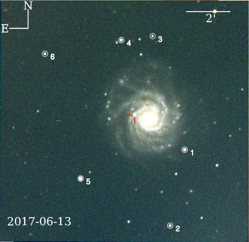
Figure 1: A pseudo-color finder chart of SN 2017ein and its host galaxy NGC 3938, produced from the $BVRI$-band images obtained with the Tsinghua-NAOC 0.8-m telescope on 2017 June 13. SN 2017ein is marked by red ticks. The comparison stars used for flux calibration are marked by white circles. North is up and west is right.

2 Observations and Data Reduction

As SN 2017ein was discovered at a young phase and it is located at a relatively close distance, we triggered followup observations immediately after its discovery. This supernova was observed in both optical and ultraviolet (UV) bands with the Swift-UVOT (Roming et al., 2005; Gehrels et al., 2004).

2.1 Optical and ultraviolet photometric obervations

Photometric observations of SN 2017ein were collected with several telescopes, including the 0.8-m Tsinghua University-NAOC telescope (TNT, Huang et al., 2012) at Xinglong Observatory of NAOC, the AZT-22 1.5-m telescope (hereafter AZT) at Maidanak Astronomical Observatory (Ehgamberdiev, 2018). The TNT and AZT observations were obtained in standard Johnson-Cousin $BVRI$ bands. These observations covered the phases from MJD 57904 (2017 May 31) to MJD 58170 (2018 Feb. 22). At late times, the supernova is only visible on the $R$- and $I$-band images on MJD 58107 (2017 Dec. 20) and becomes undetectable after that.

ATLAS is a twin 0.5-m telescope system that surveys in cyan (c) and orange (o) filters (Tonry et al., 2018). The typical sky coverage is once every 2 nights. ATLAS monitored the field of SN 2017ein from 2017 Apr. 26, and it did not detect any flux excess relative to the background until 2017 May 25.33 when the SN became detectable at an AB magnitude of 18.43$\pm$0.10 mag in the c-band, which is about 0.64 day before the first discovery. The SN was also detectable in the o-band image taken on 2017 May 27.25. Figure 2 shows the ATLAS $c$-band prediscovery and the earliest detection images of SN 2017ein. The ATLAS observations of SN 2017ein lasted until 2017 July 03. The ATLAS data are reduced and calibrated automatically as described in (Tonry et al., 2018). The photometry was done on the difference images by subtracting pre-explosion templates. A model of the point-spread-function (PSF) was created and fitted to the excess flux sources in the images (as described in Tonry et al., 2018). The photometric calibration was achieved with a custom-built catalogue based on the Pan-STARRS reference catalogues (Magnier et al., 2016), and the magnitudes are in the AB system.

All $BVRI$ CCD images were pre-processed using standard IRAF routines, which includes corrections for bias, flat field, and removal of cosmic rays. As SN 2017ein exploded near a spiral arm of the host galaxy, the late-time photometry may be influenced by contamination from the galaxy. We thus use the template images taken on 2018 Jun. 16 and 18 (which correspond to $\sim+$390 days from the discovery) to get better photometry for the AZT images taken at late phases when the supernova was relatively faint. We did not apply template subtraction to the TNT images as the SN is bright relative to the galaxy background when these images were taken. The instrumental magnitudes of both the SN and the reference stars were then measured using the standard point spread function (PSF). These magnitudes were converted to those of the standard Johnson system using the Pan-STARRS reference catalogue. The magnitudes of the comparison stars used for flux calibration, as marked in Figure 1, are listed in Table 1. Although the supernova is not visible in images taken after MJD 58107, we also measured the magnitudes at the supernova site. These measurements provide upper limits of the late-time light curves. The final flux-calibrated magnitudes (Vega) of SN 2017ein from TNT and AZT are shown in Table 7, and the photometric results (AB magnitudes) from ATLAS are reported in Table 8.

SN 2017ein was also observed with the Ultraviolet/Optical Telescope (UVOT; Roming et al., 2005) onboard the Neil Gehrels Swift Observatory (Gehrels et al., 2004). The observations were obtained in uvw1, uvm2, uvw2, $u$, $b$, and $v$ filters, from 2017 May 27 until 2017 July 21. The Swift/UVOT data reduction is based on that of the Swift Optical Ultraviolet Supernova Archive (SOUSA; Brown et al., 2014). A 3″ aperture is used to measure the source counts with an aperture correction based on an average PSF. Magnitudes are computed using the zeropoints from Breeveld et al. (2011) for the UV and Poole et al. (2008) for the optical and the 2015 redetermination of the temporal sensitivity loss. The photometry is performed on the images subtracted by the template that was obtained on 2018 Jun. 02. The supernova was visible only in uvw1 band but not in uvw2 and uvm2 bands, likely due to the significant reddening that it suffered from the host galaxy (see discussion in Section 4). The Swift-UVOT photometry is listed in Table 9. The UVOT $b$- and $v$-band photometry are comparable to those of the ground-based observations around peak in $B$ and $V$ bands, respectively, while the UVOT photometry suffered large uncertainties at later phases.

Table 1: Magnitudes of Comparison Stars in Field of SN 2017ein.

Star No.	R.A.	Decl.	B	V	R	I
1	11h52m40s.50	44°05′49′′.41	15.848$\pm$0.037	15.067$\pm$0.013	14.611$\pm$0.015	14.194$\pm$0.016
2	11h52m44s.22	44°02′20′′.76	16.490$\pm$0.035	15.774$\pm$0.012	15.354$\pm$0.015	14.927$\pm$0.016
3	11h52m48s.69	44°11′01′′.51	16.879$\pm$0.037	16.442$\pm$0.013	16.173$\pm$0.015	15.865$\pm$0.016
4	11h52m56s.69	44°10′50′′.83	15.874$\pm$0.036	15.166$\pm$0.013	14.750$\pm$0.015	14.337$\pm$0.016
5	11h53m07s.08	44°04′30′′.23	14.386$\pm$0.036	13.843$\pm$0.013	13.516$\pm$0.015	13.149$\pm$0.016
6	11h53m16s.23	44°10′13′′.08	16.880$\pm$0.039	16.009$\pm$0.016	15.504$\pm$0.017	15.052$\pm$0.017

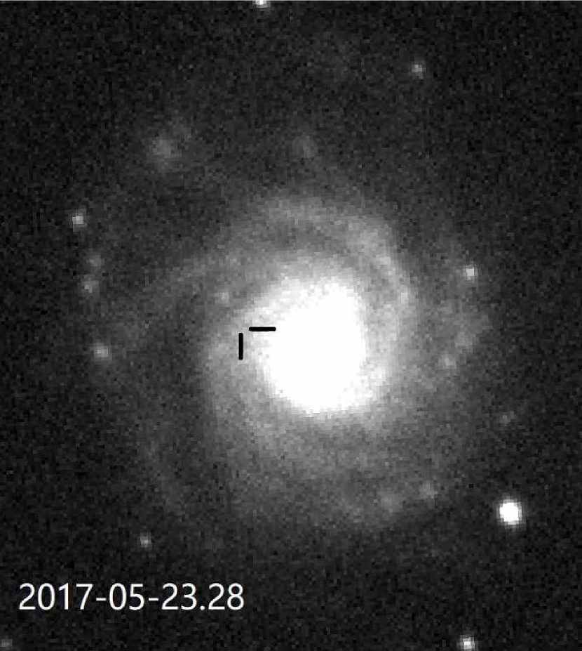
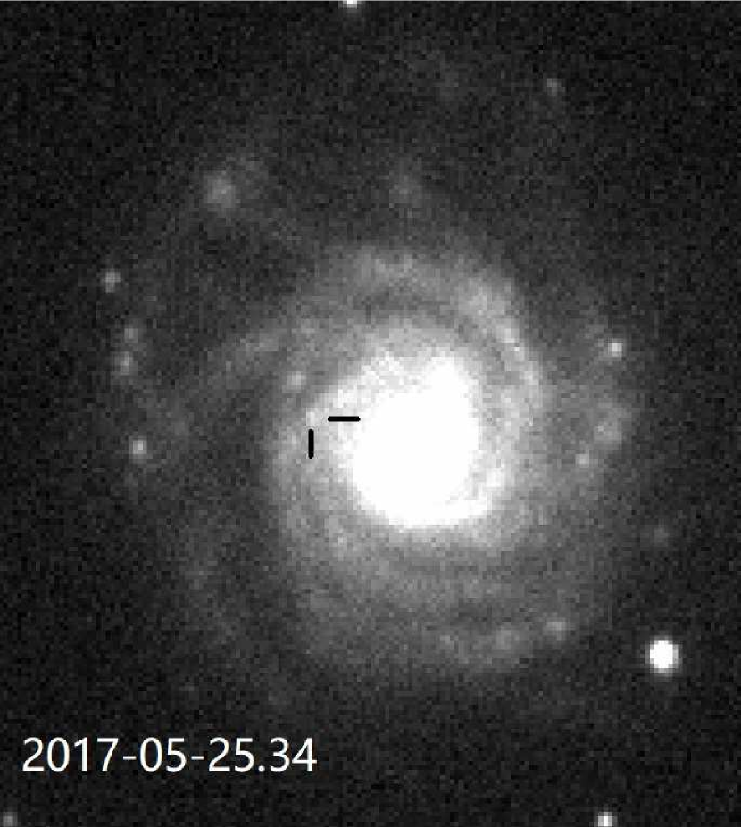
Figure 2: The ATLAS images centering at the galaxy NGC 3938, north is up and west is right. left: The latest non-detection image taken on 2017 May 23.28 in o-band. The AB magnitude at the SN position is fainter than 20 mag (after subtracting template); middle: the first detection image of SN 2017ein on 2017 May 25.34 in c-band; right: residual image obtained by subtracting the template from the first-detection image, with the position of the SN marked.

2.2 Optical spectroscopy

Our first spectrum of SN 2017ein was obtained on UT 2017 May 26.57 with the Xinglong 2.16-m telescope of NAOC (hereafter XLT), which is at $\sim$2.5 days after explosion, assuming that the explosion date is 2017 May 24.0 according to the analysis conducted in Section 6. A sequence of 9 low-resolution spectra were collected with different telescopes including the XLT, the Lijiang 2.4-m telescope (hereafter LJT), the ARC 3.5-m telescope at Apache Point Observatory (hereafter APO 3.5-m), the 2-m Faulkes Telescope North (FTN) of the Las Cumbres Observatory network, and the 9.2-m Hobby-Eberly Telescope (HET). The details of the spectroscopic observations are listed in Table 2.

All spectra were reduced using the standard IRAF routines, which involves corrections for bias, flat field, and removal of cosmic rays. The Fe/Ar and Fe/Ne arc lamp spectra obtained during the observation night are used to calibrate the wavelength of the spectra, and standard stars observed on the same night at similar airmasses as the supernova were used to calibrate the flux of spectra. The spectra were further corrected for continuum atmospheric extinction during flux calibration, using mean extinction curves obtained at Xinglong Observatory, Lijiang Observatory, Apache Point Observatory, and Haleakala Observatory in Hawaii; moreover, telluric lines were removed from the data.

Table 2: Journal of Optical Spectroscopy of SN 2017ein.

UT	MJD	$t_{e}$	$t_{V}$	Telescope	Instrument	Exposure time (s)
2017/05/26.57	57899.57	2.6	$-13.9$	BAO 2.16 m	BFOSC+G4	3600
2017/05/30.63	57903.63	6.6	$-9.9$	BAO 2.16 m	BFOSC+G4	3000
2017/05/31.60	57904.60	7.6	$-8.9$	BAO 2.16 m	BFOSC+G4	3000
2017/06/15.15	57919.15	21.7	$+5.2$	HET 9.2 m	LRS2	1500
2017/06/20.56	57924.56	27.5	$+11.0$	BAO 2.16 m	BFOSC+G4	2700
2017/06/23.29	57927.29	30.3	$+13.8$	FTN 2.0 m	FLOYDS	2700
2017/06/28.28	57932.28	35.3	$+18.8$	FTN 2.0 m	FLOYDS	2700
2017/07/29.55	57963.55	66.5	$+50.1$	LJO 2.4 m	YFOSC+G10	2100
2017/08/21.04	57987.04	90.0	$+73.6$	APO 3.5 m	DIS+B300&R400	1800

3 Photometric Properties of SN 2017ein

3.1 Optical and ultraviolet light curves

Figure 3 shows the AZT and TNT BVRI light curves of SN 2017ein, in comparison with those of SN 2007gr (Chen et al., 2014). The Swift UVOT $uvw1$- and $ubv$-band light curves are also overplotted. Applying polynomial fits to the data around maximum light, we found that SN 2017ein reached $B$-band peak of m_B(peak)=15.91$\pm$0.04 mag on MJD 57909.86, and $V$-band peak of m_V(peak)=15.20$\pm$0.02 mag at $\sim$3.6 days later. This gives an estimate of $B_{\mathrm{max}}-V_{\mathrm{max}}$ color as 0.71$\pm$0.05 mag for SN 2017ein, which is much redder than the typical value for normal SNe Ic. Given the small reddening of E$(B-V)_{\mathrm{MW}}$=0.019 mag due to the Milky Way (Schlafly & Finkbeiner, 2011) and a typical $B-V$ color of 0.4 mag for normal SNe Ic near the maximum light (Drout et al., 2011), the red color observed for SN 2017ein indicates that it suffered significant reddening due to the host galaxy (see also discussion in Section 4).

In Figure 4, we compare the $BVRI$-band light curves of SN 2017ein to those of other well observed SNe Ib/c. SN 2017ein shows light curves that are very similar to SN 2007gr in all four $BVRI$ bands before t$\sim$+60 days from the peaks. Adopting the explosion date as MJD 57897.0 obtained in Section 6, we find a rise time of $\sim$13.2 days in the $B$ band and $\sim$16.6 days in the $V$ band for SN 2017ein. This rise time is longer than that of SN 1994I and SN 2004aw, but similar to that of SN 2007gr and SN 2013ge. Moreover, we also measured the post-peak magnitude decline-rate parameter $\Delta m_{15}$, which is derived as 1.33$\pm$0.07 mag in $B$ and 0.93$\pm$0.04 mag in $V$ respectively for SN 2017ein. These values are nearly equal to those measured for SN 2007gr ($\Delta m_{15}(B)$=1.31 mag; Chen et al., 2014) and slightly larger than those for SN 2013ge ($\Delta m_{15}(B)$=1.11 mag; Drout et al., 2016). The full light-curve parameters in different bands are listed in Table 3. Our observations did not cover the period from t$\sim$60 – 190 days after $V$-band maximum due to solar conjunction. The later observations restarted on MJD 58107, corresponding to a phase of t$\sim+$193 d with respect to the $V$ maximum. The supernova became too faint to be detectable except in $R$- and $I$-bands, where SN 2017ein is found to be apparently fainter than SN 2007gr at this phase. Due to the absence of observations during t$\sim+$60 – 190d, it is unclear when the light curves of SN 2017ein started to deviate from those of SN 2007gr.

Figure 4 shows the comparison of SN 2017ein with some well-observed SNe Ibc including SNe 1994I, 2002ap, 2004aw, 2007gr, 2008D, and 2013ge. The upper limits showing obvious large deviations from the evolutionary trend are due to improper subtraction and bad weather and are not plotted. The overall light curve evolution of SN 2017ein shows close resemblance to that of SN 2007gr at t $<$ +60 days from the peak, while in the nebular phases it clearly shows a much faster decline than SN 2007gr and other SNe Ib/c with similar light curve shapes near maximum light. On day MJD 58107, SN 2017ein is found to be fainter than SN 2007gr by $\sim 0.9$ mag in $I$-band and $\sim 0.4$ mag in $R$-band, respectively. The relatively slower decline in the $R$ band is probably due to a contribution of O I, O II, and Ca II emission in the nebular phases. For SN 2007gr, Chen et al. (2014) found that it dimmed at a pace faster than the ⁵⁶Co decay in all bands after $t\sim+80$ d from the peak, which can be explained with an increase of escape rate of $\gamma$-rays at this phase; and its $R$-band light curve also showed a relatively slower evolution than other bands. Thus, the faster decay seen for the late-time light curves of SN 2017ein could be due to larger escape rate of the $\gamma$ photons, suggestive of a low ejecta mass for SN 2017ein (see also discussion in Section 6). Alternatively, the newly formed dust in the cooling ejecta may also shed light from the supernova.

Figure 3: $BVRI$ light curves of SN 2017ein, obtained with the 0.8-m Tsinghua-NAOC telescope, AZT-22 1.5-m telescope, and Swift UVOT. The vertical dashed line marks the maximum time in the $V$ band. The ticks at the bottom mark the epoches with spectroscopic observations. Also plotted are the $BVRI$ light curves of SN 2007gr (Chen et al., 2014). The light curves of SN 2007gr are shifted in time and magnitudes to match the corresponding light curve peaks of SN 2017ein.

Table 3: Light-curve Parameters Obtained for SN 2017ein.

band	peak date (MJD)	peak obs. mag.	peak abs. mag.	$\Delta m_{15}$(mag)
$B$	57909.86$\pm$0.24	15.91$\pm$0.04	$-17.20\pm 0.38$	1.33$\pm$0.07
$V$	57913.49$\pm$0.20	15.20$\pm$0.02	$-17.47\pm 0.35$	0.93$\pm$0.04
$R$	57914.67$\pm$0.28	14.81$\pm$0.05	$-17.54\pm 0.33$	0.75$\pm$0.09
$I$	57916.32$\pm$0.30	14.43$\pm$0.04	$-16.93\pm 0.32$	0.61$\pm$0.09

Figure 4: Comparison of $BVRI$ light curves of SN 2017ein with other SNe Ib/c: SN 1994I, SN 2002ap, 2004aw, 2007gr, SN 2008D and SN 2013ge. The light curves are shifted in time and magnitude to match the peaks of SN 2017ein. Data references: SN 1994I (Richmond et al., 1996; Yokoo et al., 1994), SN 2002ap (Foley et al., 2003), SN 2004aw (Taubenberger et al., 2006), SN 2007gr (Chen et al., 2014), SN 2008D (Mazzali et al., 2008; Modjaz et al., 2009; Bianco et al., 2014; Brown et al., 2014), and SN 2013ge (Drout et al., 2016).

The color evolution of SN 2017ein and the comparison sample is presented in Figure 5, where all color curves have been corrected for the total reddening to the supernova. The colors derived from the earliest two spectra are also included in the plot. For SN 2017ein, a total reddening of E$(B-V)$$\sim$0.42 mag derived in the next section is removed from the color curves. As can be seen, all color curves seem to follow a similar trend, evolving bluewards from t$\sim$2 weeks to a few days before the $V$-band maximum. Note that the $B-V$ and $B-R$ colors of SN 2008D are very blue at t $\lesssim$ 2 weeks before $V$-band maximum and they evolve redwards quickly, suggestive of an initial high temperature that can been interpreted as shock heating or interaction (Modjaz et al., 2009; Mazzali et al., 2008). This feature is also observed in the color evolution of SN 2017ein, suggesting that its early-time emission may have also experienced a cooling stage of shock breakout emission. We will further investigate this feature in Section 6.

After reaching the bluest color, all color curves become progressively red until 3 weeks after maximum, followed by a plateau phase. The $B-V$ color curves of different SNe Ib/c tend to converge at $\sim$0.5 mag near maximum light, though they show relatively large scatter before and after the peak. The $V-R$ color shows a similar trend, and it tends to converge at $\sim$0.2–0.3 mag at about 10 days from $V$ band maximum as suggested by Drout et al. (2011). SN 2017ein shows color evolution that overall is quite similar to SN 2007gr.

Figure 5: Color evolution of SN 2017ein and some well-observed SNe Ic, all corrected for the Galactic and host-galaxy reddening. The color curve of SN 2008D (SN Ib) is overplotted for comparison. The open circles represent the synthetic color derived from the spectra. The dashed lines mark that the V R color tends to have a uniform value of $\sim 0.26$ in Drout et al. (2011) at t$\sim$+10 days from the $V$-band maximum. Data references are the same as in Figure 5.

3.2 The early light curves from ATLAS

The survey observation of ATLAS is operated in two specifically designed bands, ATLAS-cyan ($c$) and ATLAS-orange ($o$) (Tonry et al., 2018). Figure 6 shows the transmission curves of these two filters and the broadband $BVRI$-band filters. One can see that the ATLAS $o$ and $c$ filters have similar effective wavelengths to the broadband $R$ and $V$ filters, respectively. To examine the difference between them, we calculate the synthetic $c-V$ and $o-R$ colors using the spectra of SN 2017ein presented in this paper, and those from Van Dyk et al. (2018). The results are shown in Figure 7. The $V$-band magnitudes appear slightly brighter than those in $c$-band by $\sim$0.2 mag, and this difference tends to be smaller in the early and late phases (see the left panel of Figure 7). The ATLAS-$o$ magnitude differs from the $R$-band value at the same phase by $\sim$0.15 mag, as shown in the middle panel of Figure 7; and in very early phase this difference is less than 0.1 mag. In the right panel of Figure 7, we show the evolution of the ATLAS $c-o$ color for SN 2017ein, with the $c$-band magnitudes being fainter than the $o$-band by 0.2–0.8 mag. A low-order polynomial fit is applied to the $c-V$, $o-R$, and $c-o$ color evolutions, and the best-fit result is then used to interpolate the magnitudes in different bands when necessary.

Figure 8 shows the ATLAS $o$-band light curves (AB magnitude) of SN 2017ein, together with those converted from the AZT and TNT $R$-band photometry using the $o-R$ relationship shown in Figure 7. In the conversion, we added a systematic error of 0.03 mag to the converted magnitude errors. And the converted light curve is shifted by 0.13 mag to match the peak of the $o$-band light curve. The earliest prediscovery detection from the ATLAS $c$-band observation, taken on 2017 May 25, is also plotted for comparison. In this plot, we also include the magnitude derived from our first spectrum taken on 2017 May 26.57. This spectrum was flux-calibrated using the first $R$-band photometry from AZT (taken on 2017 May 25.77) and the earliest ATLAS $o$-band photometry (taken on 2017 May 27.26). The earliest $R$-band photometry was reported in Im et al. (2017) with a magnitude of 17.7 mag on MJD 57898.77. We obtained the raw images through private communication and reduced the data with our pipeline ZrutyPhot (Mo et al. in prep.) and obtain a magnitude of 17.78$\pm$0.01 mag. This measurement is converted to the $o$-band magnitude and included in our analysis as well. The latest non-detection is from the 1-m telescope at Deok-Heong Optical Astronomy Observatory (DOAO) in South Korea, which gives an $R$-band limit of $>$18.4 mag from images taken on 2017 May 24.63 (Im et al., 2017), which is transformed to the AB system and also plotted in Figure 8.

These early-time data can be used to constrain the time of first-light for SN 2017ein. Using the data points before MJD 57907 and adopting a function of luminosity evolution as $L(\lambda)\propto t^{n}$ in the fit, we find the explosion date of MJD 57897.2$\pm$0.6 by fitting the early the TNT and AZT $R$-band data. To get better data sample, especially at early times, we also combine the converted $R$-band data with the ATLAS $o$-band data together to infer the explosion time as MJD 57896.8$\pm$0.3 (see Figure 8). However, we caution that such a combined analysis may suffer some uncertainty due to that the conversion between these bands is not very accurate. These estimated dates are very close to the non-detection date MJD 57896.77 presented by Im et al. (2017), with $R$>19.9 mag. Thus, the explosion date should be near MJD=57896.9, with a 1-$\sigma$ error of 0.3 day. The corresponding power-law index for the above fits is $n$=1.36 and 1.51, respectively, which are smaller than the typical value of $n=2$ for the fireball model. A more detailed analysis of the explosion date is presented in Section 6, which makes use of the whole range of the light curves.

As SN 2017ein tends to have relatively bluer $c-o$ color in the early phase after explosion (see Figure 7), we assume a $c-o$ color of $\sim$0.3 mag according to the $c-o$ evolution (Figure 7). The $o$-band magnitudes are thus inferred from the corresponding $c$-band photometry and are shown as empty circles in Figure 8. When the supernova was first detected in $c$ band at t$\sim-$15.15 days from the maximum light, it showed an excess emission beyond the power-law model. This serves as an indication for possible detection of shock breakout cooling as addressed in section 6.

Figure 6: The transmission functions of the two ATLAS filters, compared with the Johnson BVRI filters.

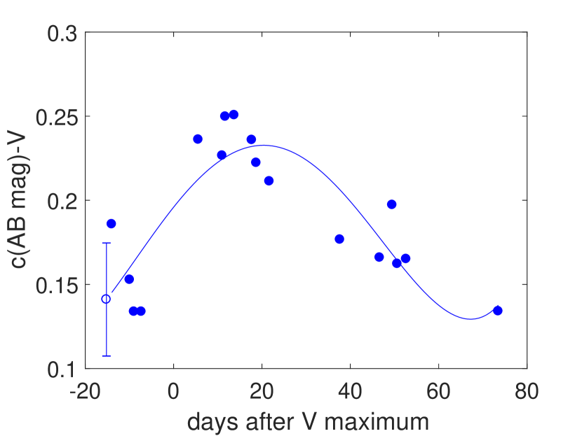
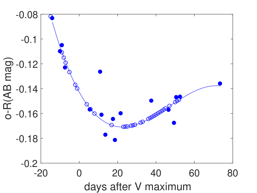
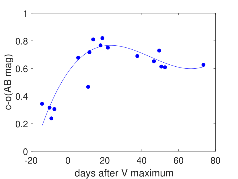
Figure 7: left: The $c-V$ (left), $o-R$ (middle), and $c-o$ (right) color evolutions of SN 2017ein, obtained using the supernova spectra presented in this paper and those taken from Van Dyk et al. (2018). The solid lines in each panel are the lower-order polynomial fits to the observed data. The open circle with an error bar is the $c-V$ color at the ATLAS-$c$ photometry epoch which is used to transform the $c$ magnitude to $V$ magnitude. The open circles in the middle panels represent the fitting values at the $R$ band photometry epochs, which are used to convert the $R$ band magnitudes to $o$ magnitudes.

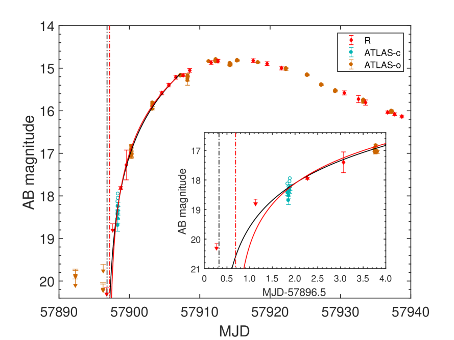
Figure 8: The ATLAS $c$ and $o$-band light curves of SN 2017ein. The $R$-band light curves from the TNT and AZT transferred to $o$-band light curves using the relation derived in Figure 7 are also overplotted. The detection limits from ATLAS and the report in Im et al. (2017) are shown by red downward arrows. The red line shows the power-law fit ($f\propto t^{n}$) to the pre-maximum $R$-band data, while the black line represents the fit to the combined data from ATLAS, AZT, and TNT. The corresponding best-fit explosion dates are shown by the vertical dot-dashed lines. The empty symbols in blue show the estimated magnitudes in $o$ band at epochs with $c$-band observations. The embedded plot shows the zoomed-in early-time light curve and the fitting.

4 Distance, Reddening and Absolute Magnitude

The distance to the host galaxy of NGC 3938 (and hence SN 2017ein) was estimated by three methods. One is based on the standardization of SNe II through an empirical relation between photospheric magnitude and color (Rodríguez et al., 2014), which is calibrated using SNe II with Cepheid distances. With the observed parameters of the SN IIP exploded in NGC 3938, SN 2005ay, a distance of 31.75$\pm$0.24 mag and 31.70$\pm$0.23 mag can be derived for this galaxy, by using the $V$ and $I$-band data respectively. While a smaller value of 31.27$\pm$0.13 mag was obtained when using correlation between luminosity and photospheric velocity of SNe IIP (Hamuy & Pinto, 2002; Poznanski et al., 2009). A smaller value of 31.15$\pm$0.40 mag can be inferred from the Tully-Fisher relation if the Hubble constant is adopted as 75 km s^-1 Mpc^-1 (Tully, 1988). In contrast to adopting a distance modulus in a range from 31.15 to 31.75 mag (see Van Dyk et al., 2018), we adopt an average (not weighted) value of 31.38$\pm$0.30 mag for the distance modulus throughout this paper.

The red peak $B-V$ color and the red spectra at early epoches both suggest that SN 2017ein suffered severe reddening from the host galaxy. We estimated the exact reddening through the Na I D absorption detected in the spectra. A moderately strong NaID absorption with an equivalent width (EW) of 2.48$\pm$0.35Å can be inferred from the spectra of SN 2017ein taken by 2-m FTN telescope with good signal-to-noise ratio (SNR). Based on the relation of E$(B-V)$ and EW of Na I D (Turatto et al., 2003), i.e., E$(B-V)$=0.16$\times$EW(Na I D), the host-galaxy reddening is thus estimated to be E$(B-V)_{\mathrm{host}}=0.40\pm 0.06$ mag.

On the other hand, a systematic statistical study of SNe Ib/c light curves (Drout et al., 2011) concludes that the $V-R$ color of SNe Ib/c clusters at $\sim$0.26$\pm$0.06 mag, as shown by the dashed lines in the $V-R$ color plot of Figure 5. To match this trend, the observed $V-R$ color of SN 2017ein has to be shifted by an amount of about 0.4 mag, which is consistent with that derived from the Na I D absorption. Adopting the extinction coefficient R_V = 3.1, the total extinction is estimated to be A_V=1.29$\pm$0.18 mag for SN 2017ein. With the distance and extinction values derived above, we estimate the absolute $V$-band peak magnitude of SN 2017ein as $-$17.47$\pm$0.35 mag. This value is within the range of normal SNe Ib/c, similar to SN 2007gr, SN 2013ge, SN 1994I etc., but fainter than SN 1998bw, SN 2004aw and LSQ14efd. In the comparison sample, SN 1998bw is the brightest, while SN 2008D is the faintest.

5 Optical Spectral Properties

5.1 Spectral classification

The complete spectral evolution of SN 2017ein is shown in Figure 9, spanning the phase from t$\sim-$13.9 days to t$\sim$+73.6 days relative to the $V$-band maximum light. The earliest spectrum of SN 2017ein is characterized by a prominent broad absorption line near 6200Å  which showed rapid evolution and split into two absorption features at 6100Å and 6250Å a few days later. This feature in earliest spectrum can be due to a combination of SiII $\lambda$6355 and CII $\lambda$6580 absorptions. Prominent broad absorption features can also be seen near 7400Å and 8100Å  which can be attributed to the OI triplet and the CaII NIR triplet, respectively. The weak absorption near 6950Å could also be due to CII $\lambda$7235 instead of HeI $\lambda$7267, as it disappeared near maximum light. For a SN Ib, the intensity of the main helium features will increase with time. Thus, the identification of the above features give us confidence to classify SN 2017ein as a type Ic supernova. This classification is further justified by the fact that it closely resembles two typical SNe Ic, SN 2007gr and SN 2013ge, as presented in Section 5.2.

Figure 9: Optical spectra of SN 2017ein. Different colors indicate spectra taken by different telescopes: XLT (black), HET (blue), FTN (magenta), LJT (red), and APO 3.5-m telescope (dark green). The spectral wavelength is in the rest-frame of the host galaxy (corrected for a redshift z=0.0027), and the flux is plotted in logarithmic scale and shifted vertically for better display. The numbers beside each spectrum shows the day after explosion and numbers in bracket represent the phase in days relative to the $V$-band maximum. The positions of some noticeable absorption features are marked by dashed lines. The H$\alpha$ line from the host galaxy is marked out.

5.2 Spectral evolution

In this subsection, we examine the spectral evolution of SN 2017ein in comparison with other SNe Ib/c at several phases. Most of the spectra of the comparison SNe are obtained via the Open Supernova Catalog (OSC; Guillochon et al., 2017). All spectra have been corrected for host-galaxy redshift and the total line-of-sight extinction using the extinction law of the Milky Way with R_V=3.1 (Gordon et al., 2003).

Figure 10 shows the comparison of pre-maximum spectra. The broad absorption feature near 6200Å at t$\sim-$13.9d evolved into two separate narrow absorption features at t$\sim-$10d. Assuming that these two features correspond to SiII $\mathrm{\lambda}$6355 and CII $\mathrm{\lambda}$6580 absorptions, they have an expansion velocity of about 10,500 km s^-1 and $12,000\mathrm{\ km\ s^{-1}}$, respectively. The identification of prominent CII $\mathrm{\lambda}$6580 absorption in the t$\sim-$10 day spectrum is supported by the presence of another absorption feature near 6950Å that can be attributed to CII $\mathrm{\lambda}$7235 with a similar blueshifted velocity. This is also confirmed by the SYNAPPS fit, with input of CII, OI, NaI, MgII, SiII, CaII, and the singly-ionized iron group elements. The fitting result is shown in Figure 11. Thus in the t$\sim-$13.9 day spectrum, the SiII and CII lines likely blended together. Applying a double gaussian fit to decompose these two features, they are found to have velocities of $\sim$14,000 km s^-1 (SiII $\lambda$6355) and $\sim$16,000 km s^-1 (CII $\lambda$6580), respectively.

The pre-maximum spectra features of SN 2017ein closely resembles those of SN 2007gr and SN 2013ge, which are all characterized by prominent, narrow CII $\mathrm{\lambda}$6580 absorption and weak SiII $\lambda$6355 absorption compared with SN 1994I. The presence of high-velocity carbon in SN 2017ein indicates that the outer part of its progenitor star should have abundant carbon, consistent with a WC-type Wolf-Rayet progenitor star that has lost its H and He envelopes and remains a bare CO core before explosion.

The comparison of the post-maximum spectra is shown in Figure 12. A late-time spectrum of type IIb SN 1993J is also overplotted. As one can see, SN 1993J has a strong $\mathrm{H\alpha}$ line near 6150Å, and the type Ib SN 2004gq and SN 2008D have several significant lines at 4300Å, 5600Å, 6500Å and 6800Å  which can be attributed to HeI. All these features are absent in SN 2017ein. After maximum light, the spectra of SN 2017ein are also similar to those of SN 2007gr and SN 2013ge except for the CaII NIR triplet. As can be seen in Figure 12, the CaII absorption feature in SN 2017ein splits into two narrow lines since t$\sim$$+$19d, which is not seen in other comparison SNe Ib/c. This is also seen in the late spectra of SN 1993J (Barbon et al., 1995). In previous studies, these two lines are both attributed to the CaII NIR triplet. In most cases, the SN photosphere is optically thick to absorption lines, and thus the adjacent lines are likely to blend and become unresolved. One example is the CaII $\mathrm{\lambda\lambda\lambda}$8498, 8542, 8662, which usually blend together into one broad line. These lines get narrower when the photosphere becomes more transparent and recedes to lower velocities. In this case, the line CaII $\mathrm{\lambda}$8662 splits from the other two CaII NIR lines. Another understanding of the split feature is that the absorption line on the right is not related to CaII NIR triplet but be due to CI $\lambda$8727 as the neutral carbon line may become stronger as a result of photospheric cooling.

Figure 10: The early-phase spectra of SN 2017ein, compared with those of SN 1994I (Filippenko et al., 1995), SN 1998bw (Patat et al., 2001), SN 2007gr (Valenti et al., 2008), SN 2008D (Modjaz et al., 2009), and SN 2013ge (Drout et al., 2016). Spectra of SN 2017ein are plotted with red color. Different colors represent different SN types: black for Ic, blue for Ib, and magenta for IIb.

Figure 11: SYNAPPS fit to the spectrum of SN 2017ein at t = $-$9d relative to $V$-band maximum. Also plotted the spectrum at -10d and spectrum of SN 2007gr at t = $-$9d relative to $V$-band peak (Valenti et al., 2008). The HeI feature in the spectrum of SN 2007gr proposed by Chen et al. (2014) is marked out.

Figure 12: Comparison of the post-peak spectra between SN 2017ein and other SNe Ib/c. The CaII NIR triplet feature is marked by grey shaded area. The line colors are the same as in Figure 10. Data references: SN 1993J (Barbon et al., 1995), SN 1994I (Filippenko et al., 1995), SN 2004gq (Modjaz et al., 2014), SN 2007gr (Valenti et al., 2008), and SN 2013ge (Drout et al., 2016).

5.3 Velocity evolution

We measured the ejecta velocity inferred from different absorption lines in the spectra of SN 2017ein. Figure 13 shows the velocity evolution of FeII $\lambda$5169, SiII $\lambda$6355, CII $\lambda$6580, OI $\lambda$7774, and CaII NIR triplet lines. The velocity of CaII NIR triplet is obviously higher than other lines, which is common for SNe since calcium has a larger opacity at the same radius and CaII absorption lines thus traces the outer layers of the ejecta at higher velocity.

Figure 14 compares line velocities with some representative SNe Ic, including SNe 1994I, 1998bw, 2002ap, 2004aw, 2007gr, and 2013ge. It is apparent that SNe Ic-BL have much higher SiII velocity from very early phases until maximum light. The ejecta velocity of SN 2017ein shows similar evolution to other normal SNe Ic like SN 2007gr and SN 2013ge, which drops rapidly in about 10 days from explosion and then remains roughly constant in later phases. Among SN 2013ge, SN 2007gr and SN 2017ein, SN 2007gr has the lowest SiII and NaI velocity in the early fast-decreasing stage. But the NaI velocity of SN 2007gr shows a re-increasing trend at later epochs. In comparison with other SNe Ic of our sample, SN 2017ein has a lower CaII velocity, e.g., $\sim$12,000 km s^-1 versus $\sim$14,000 km s^-1 at around maximum light. This difference may be caused in part by a different method of measuring the line velocity. In SN 2017ein, the CaII absorption splits into two narrower lines, and we measured the velocity from CaII $\lambda$8538 absorption instead of treating it as a blended trough of $\lambda$8571. Whereas we can not perform such a measurement for other SNe Ic of our sample because their CaII NIR features blended into one broad absorption feature.

It is noteworthy that the velocity of the Na I D line of SN 1994I showed an obvious increase from t$\sim$27 days to t$\sim$40 days from the explosion and reached a velocity plateau after that. The NaI velocity inferred for SN 2007gr seems to have a similar trend of evolution, but with much lower plateau velocity. As discussed in Hunter et al. (2009), this is probably related to the combination of NaII to NaI or the departure from LTE to NLTE, although this trend could be also caused by contamination with HeI $\lambda$5876. The latter scenario gets support from recent studies that residual He may exist in some SNe Ic (e.g. Chen et al., 2014; Prentice et al., 2018). While Chen et al. (2014) suggested that in the early-time spectra of SN 2007gr, the feature near 5500Å, bluewards of Na I  D line, should be attributed to HeI (see their Figure 7), our fitting of the spectrum shows that this feature of SN 2017ein can be produced without adding a contribution from He (see Figure 11).

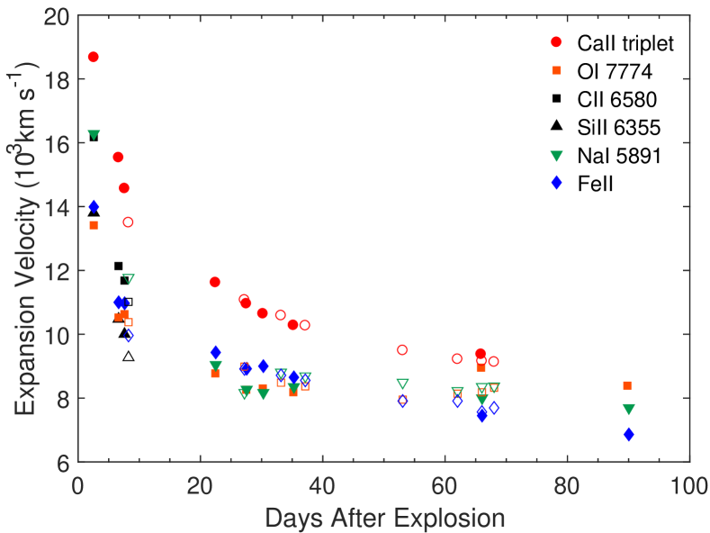
Figure 13: Expansion velocity inferred from absorption lines in the spectra of SN 2017ein. The open symbols represent the data measured from the spectra in Van Dyk et al. (2018).

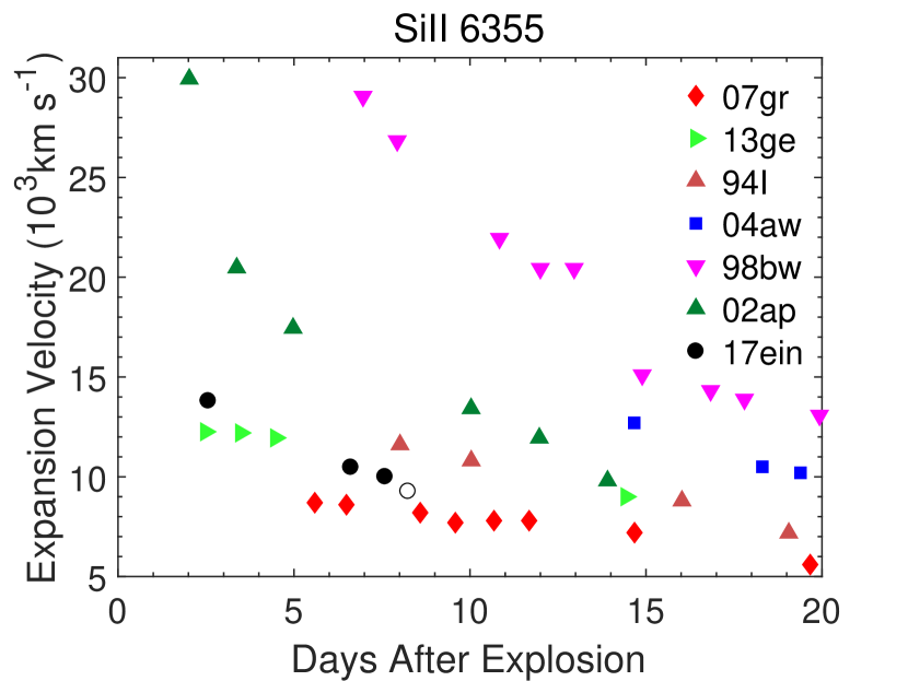
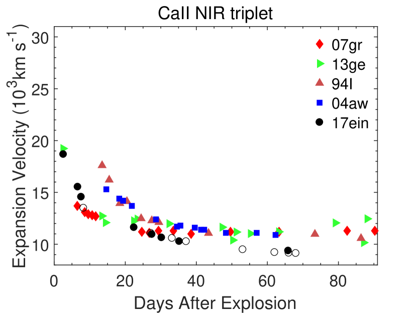
Figure 14: Evolution of the ejecta velocity inferred from SiII $\lambda$6355 (left), CaII NIR triplet $\lambda$8571 (middle), and NaID $\lambda$5891 (right) in the spectra of SN 2017ein and some well-observed SNe Ic. The open circles represent the measurement for SN 2017ein using spectra from Van Dyk et al. (2018).

6 Shock Breakout Cooling

In this section, we perform a quantitative analysis of the overall evolution of the light curves to investigate the explosion parameters of the supernova and properties of its progenitor. The observation data include the $BVR$-bands light curve from AZT, Swift UVOT, and TNT, and the earliest detection from ATLAS in $c$-band. The light curves of SNe Ic are usually believed to be powered by radioactive decay of ⁵⁶Ni and ⁵⁶Co (Arnett, 1982), though the magnetar model has recently been proposed to account for some subclasses of SNe Ic such as SNe Ic-BL (e.g. Wang et al., 2017, 2016; Kasen & Bildsten, 2010) and super luminous supernovae (SLSNe). We note the possible excess emission compared to the power-law fit in the early light curves of SN 2017ein (see Section 3.2), and the similar color evolution with SN 2008D during the first one or two days after explosion (see Figure 5). Given the short duration of these features, it is possible that the early light curve of SN 2017ein is related to the cooling of the shock breakout. So we model the light curves by including a component due to shock cooling.

During the cooling phase, the light curve is dominated by cooling emission from shock breakout (Piro, 2015; Piro & Nakar, 2013). This shock cooling model considers a thermodynamical solution of the variation of the luminosity, which is related to energy, mass, and radius of the surrounding material, and expanding velocity of the shocked envelope. The analytical model given by Arnett (1982) can be utilized to compute the bolometric luminosity. Due to the lack of good UV and IR light curve samples, we try to fit the multiband light curves instead of bolometric light curve. To fit the multiband data, we assume a blackbody SED. Combined with the calculated photospheric radius, the effective temperature of the photosphere can be determined, by which the flux density at every band can be calculated. Then we convert the flux density into absolute magnitude.

Based on the Arnett ⁵⁶Ni-decay and shock cooling models and methods described above, we applied the MCMC method (Wang et al., 2017) to fit the observed $BVR$ multi-band light curves of SN 2017ein. The observational data include Swift UVOT, AZT, and TNT light curves, and the magnitudes derived from the first spectrum. We also convert the earliest ATLAS-c photometry to the corresponding value in the $V$-band and include it in the $V$-band light curve. Before that, the five earliest ATLAS-$c$ band data were averaged as they were taken within 1–2 hours. To transform the $c$-band magnitude to the $V$-band, we use the $c-V$ color relationship described in Section 3.2. At the epoch when ATLAS-$c$ photometry was taken, the $c-V$ value is estimated to be 0.14$\pm$0.04 mag, from a polynomial fit to the $c-V$ evolution shown in Figure 7.

In the fitting, the opacity to the ⁵⁶Ni and ⁵⁶Co decay photons is adopted as $\kappa_{\gamma,\mathrm{Ni}}=0.027\ \mathrm{cm^{2}\ g^{-1}}$, $\kappa_{\mathrm{opt}}=0.1\ \mathrm{cm^{2}\ g^{-1}}$, respectively, which are typical values for normal SNe Ic. The fitting result including only the contribution of ⁵⁶Ni decay is shown by the dotted lines in Figure 15, and one can see that it can not explain the early “bump” in the light curves despite that it fits almost the whole light curve in $V$- and $R$-bands. By fitting the light curves we also find that the photosphere cooled to a constant effective temperature of 3000$\sim$4000 K since t$\sim$40 days after explosion. To account for this phenomenon, we apply a technique similar to Nicholl et al. (2017) (see their Equation 9) so that we can also fit the late-time light curve.

The best-fit light curves are shown in Figure 15, and the resultant parameters of the supernova and the progenitor star are reported in Table 4. We do not show the $I$-band light curve because it can not be fit very well, possibly due to a larger discrepancy between the blackbody assumption and the actual SED of the supernova in the $I$ band, where the spectra of SN are dominated with strong O and Ca absorption lines. The fitted parameter $M_{\mathrm{env}}$ is the mass of the outermost shell of the star, from the stellar surface to position where the optical depth is $\sim v/c$ ($v$ is the shock velocity and $c$ the light speed). Note that $M_{\mathrm{ej}}$ is the rest of the ejected mass of the explosion, while the total ejecta mass is $M=M_{\mathrm{env}}+M_{\mathrm{ej}}$. So the total ejecta mass is $0.92\pm 0.10$ M_⊙. Our fitting gives the explosion time as MJD 57897.6$\pm$0.6, which is consistent with that derived in Section 3.2. We thus adopt the explosion time as the weighted average value of these two estimates, i.e. MJD 57897.0$\pm$0.3.

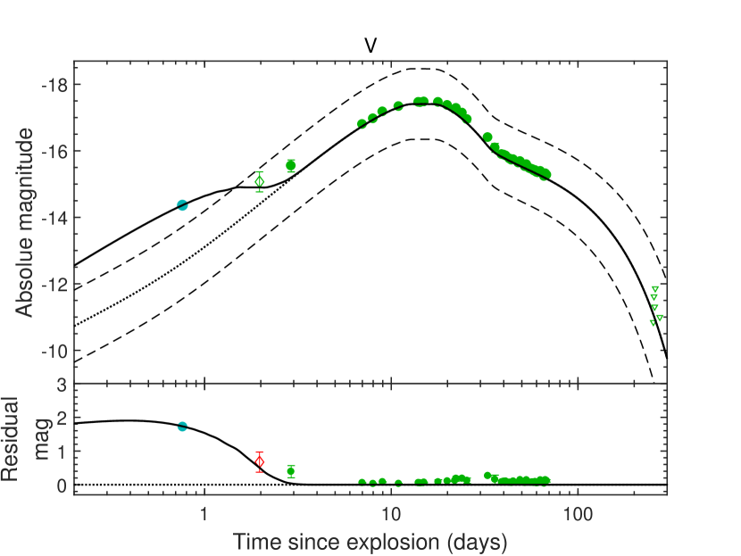
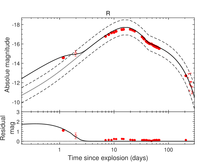
Figure 15: The fitting results of the $BVR$ light curves of SN 2017ein. Each subplot shows one band. The absolute magnitudes from ATLAS, Swift UVOT, AZT and TNT data are shown by solid symbols. The open diamond represents the magnitude derived from the first spectrum taken on 2017 May 26.57. The data point in cyan represent the magnitude converted from ATLAS $c$-band magnitudes in the $V$-band figure (see text for details). The lower panel of each plot shows the residual of the shock cooling model (solid line) and observations (data points) relative to non-cooling model.

Table 4: The explosion and progenitor parameters determined from the MCMC fit to the observed $BVR$ light curves of SN 2017ein.

$M_{\mathrm{ej}}$	$v_{\mathrm{ph}}$	$E_{K}$	$M_{\mathrm{Ni}}$	$t_{\mathrm{exp}}$	$R_{\mathrm{env}}$	$M_{\mathrm{env}}$
M⊙	$\mathrm{km\ s^{-1}}$	$10^{51}\mathrm{erg}$	M⊙	MJD	R⊙	M⊙
$0.9\pm 0.1$	9300$\pm$120	$\sim$0.5	$0.13\pm 0.01$	57897.6$\pm$0.6	8$\pm$4	$0.020\pm 0.004$

As shown in Figure 15, the early-time $V$ and $R$-band light curves of SN 2017ein can not be explained by ⁵⁶Ni heating alone. Adding the contribution from shock cooling improves the fit significantly. The first spectrum was taken at the end of the cooling tail. While the shock-cooling feature in the $B$-band is not so convincing, because there are no observations at earlier phases in this waveband when shock-cooling emission was stronger. The emission of the cooling component rises to a peak at about 0.7 day after explosion, and then fades away $\sim$3 days after explosion. After the cooling phase, the Ni-decay model well reproduces the observations. The model fit with shock cooling gives a stellar envelope radius as $R_{\mathrm{env}}$=8$\pm$4 R_⊙, which is consistent with the radius inferred from analysis of the pre-explosion images (see Section 7). This also suggests that the cooling is from the stellar envelope but not the CSM around the progenitor star. In the latter case, the distance to the outer region of the CSM should be much larger than a few R_⊙, and the cooling process will have a longer timescale and produce a more luminous cooling tail. Thus, the early excess emission detected in SN 2017ein is more likely related to shock breakout at the surface of the progenitor star.

Although the “bump” feature in the early light curve seems to be well fit by including a shock cooling contribution, it is still possible that the excess emission was caused by other processes. One popular interpretation is the mixing of ⁵⁶Ni in the outer layers of the SN ejecta, which is successful in modeling the light curves of some hypernovae like SN 1997ef (Iwamoto et al., 2000), SN 1998bw (Iwamoto et al., 1998; Nakamura et al., 2001), and normal type Ic SN 2013ge (Drout et al., 2016) and iPTF15dtg (Taddia et al., 2016). Mixing of nickel into the outer layers of SN ejecta could produce a fast rise and an extra peak or “bump” in the early phases, as well as broader shaped light curves. However, the nickel-mixing model usually has a longer timescale. For example, SN 2013ge has an extra “bump” peaking at about four days after explosion in the UV bands (Drout et al., 2016). While in SN 2017ein, the early-time flux peak appears within one day after explosion, suggestive of a lower possibility for nickel mixing on the surface of the exploding star. Recently Yoon et al. (2018) discussed the effect of Ni-mixing on the early-time photometric evolution of SNe Ib/c, and found that the color curves will become progressively red rather than showing an early peak as seen in SN 2008D and SN 2017ein (see Figure 5). We thus prefer the shock cooling model instead of nickel mixing for SN 2017ein.

The ejecta mass we estimated here as $M\sim 1\mathrm{M_{\odot}}$ is at the lower end of SNe Ib/c (Lyman et al., 2016). For comparison, the ejecta mass of SN 2007gr has been estimated in the literature, i.e., 2.0–3.5 M_⊙ by Hunter et al. (2009) and $1.8^{+0.6}_{-0.4}$ M_⊙ by Lyman et al. (2016). Hunter et al. (2009) did not describe the details of their fitting. While Lyman et al. (2016) adopts an opacity of $\kappa_{\mathrm{opt}}=0.06\ \mathrm{cm^{2}\ g^{-1}}$ in their analysis, which is smaller than the value adopted here. In the photospheric phase, the Arnett light curve model is described by two parameters: $M_{\mathrm{Ni}}$ and $\tau_{m}$, the latter is given by $\tau_{m}^{2}=\frac{2\kappa_{\mathrm{opt}}M}{\beta cv_{\mathrm{sc}}}$, where $\beta=13.8$ is a constant, $M$ is the total ejecta mass, $v_{\mathrm{sc}}$ is the scale velocity of the SN, which is observationally set as the photospheric velocity at maximum light ($v_{\mathrm{ph}}$). In our model, $v_{\mathrm{ph}}$ is given by the fit with input of the Fe II line velocities measured from the spectra. Hunter et al. (2009) found $v_{\mathrm{ph}}\approx$ 6,700 $\mathrm{km\ s^{-1}}$ from Si II line, but Lyman et al. (2016) uses $v_{\mathrm{ph}}\approx$ 10,000 $\mathrm{km\ s^{-1}}$ from Fe II line. The velocity evolution of SN 2007gr and SN 2017ein shows that the velocity used by Lyman et al. (2016) may be overestimated (see Figure 14). Using the results from Lyman et al. (2016), we find $\tau_{m}\approx 12$ d. And we obtain a similar value for SN 2017ein. Therefore, the different $M_{\mathrm{ej}}$ values inferred for SN 2007gr and SN 2017ein are mainly a result of different opacity values adopted in the analysis. Moreover, the discrepancy in the ejected mass could also be related to the fitting methods and wavebands of the light curve used in the analysis.

SN 2017ein is one of the two SNe Ic showing possible evidence for early shock breakout cooling. Another candidate is supernova LSQ14efd, with its $V$-band light curve showing a bump feature at early times, which was also interpreted as cooling of the shocked stellar envelope (Barbarino et al., 2017). In comparison with SN 2017ein, LSQ14efd is more luminous and energetic, with an $R$-band peak absolute magnitude of $-$18.14 mag, kinematic energy $E_{\mathrm{kin}}=$5.3 B, and ejecta mass $M_{\mathrm{ej}}=$ 6.3 M_⊙, respectively, making it stand between normal SNe Ic and SNe Ic-BL.

7 HST Progenitor Observation

7.1 Pre- and post-explosion HST images and data reduction

We searched the pre-explosion HST images from Mikulski Archive for Space Telescopes (MAST) and the Hubble Legacy Archive (HLA), and found publicly available F555W and F814W WFPC2 images taken on 2007 Dec. 11 (PI: W. Li). A F438W-band image at the location of SN 2017ein was taken by HST on 2017 Jun. 12 with the WFC3/UVIS configuration (PI: van Dyk). This image was released and publicly available immediately after the observation. We use this image as a post-explosion image to identify the position of the SN progenitor. Table 5 lists the information of these images.

The pre- and post-discovery HST images around the SN position are shown in Figure 16, where the zoomed-in regions centered at the SN site are also shown. There is clearly a point-like source near the SN position in both the F555W and F814W images. The position of this point-like source is obtained by averaging the measured values with four different methods (centroid, Gauss, $o$-filter center algorithm of IRAF task phot, and IRAF task Daophot). On all pre-explosion images, the separation between the position transformed from the post-explosion SN site and the center of the nearby point-like source is within the uncertainty of the transformed position, suggesting that this nearby point source is the progenitor of SN 2017ein. The coordinates of the SN on the post-explosion F438 image are found to be (539.302$\pm$0.002, 564.516$\pm$0.003) with different methods (centroid, Gauss and o-filter center algorithm of IRAF task phot, IRAF task imexamine, and SExtractor). And are converted to (798.70, 1766.77) and (798.38, 1766.67) on the pre-explosion F555W and F814W images, respectively, as the coordinates of the progenitor.

To get accurate positions of SN 2017ein on the pre-discovery images, we first chose several stars that appeared on all the post- and pre-explosion images and then got their positions on each image using SExtractor. A second-order polynomial geometric transformation function is applied using the IRAF geomap task to convert their coordinates on the post-explosion image to those on the pre-explosion images. Based on the IRAF geoxytran task, this established the transformation relationship between the coordinates of SN 2017ein on the post-explosion image and those on the pre-explosion images. The uncertainties of the transformed coordinates are a combination of the uncertainties in the SN position and the geometric transformation. The transformed SN and progenitor positions and their uncertainties are listed in Table 6. As one can see, the location of the SN center and the point-like source on the pre-explosion F555W and F814W images have small offsets of $0^{\prime\prime}.020$ and $0^{\prime\prime}.030$, respectively, which are smaller than the uncertainty of the location of the supernova.

We use DOLPHOT to get photometry of the progenitor on the pre-explosion images. The photometry is performed on raw C0M FITS images obtained from the MAST archive. Magnitudes and their uncertainties of the progenitor candidate are extracted from the output of DOLPHOT. We find that the progenitor star has magnitudes of 24.46$\pm$0.11$\ \mathrm{mag}$ and 24.39$\pm$0.17$\ \mathrm{mag}$ in F555W band and F814W band, respectively. Note that our measurements are brighter by about 0.1 mag in F555W and 0.2 mag in F814W, respectively, compared with the results recently reported by Van Dyk et al. (2018).

To further constrain the properties of the identified point-like source at the SN position, we also studied the photometric properties of the surrounding stars within 5 arc-second, corresponding to a radius of about 400 pc, around the progenitor. The measured PSF FWHMs of these stars are in a range of $0^{\prime\prime}.15\sim 0^{\prime\prime}.20$ in both F555W and F814W bands, which are consistent with that derived for the progenitor (i.e. $0^{\prime\prime}.21$ in F814W). While these FWHMs of the stars correspond to a radius of $\sim 16$pc, which is possible for a compact star cluster. So we can not be sure about whether the progenitor candidate is a single star, a multi-system, or a star cluster.

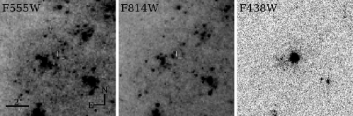
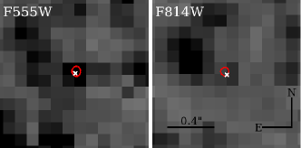
Figure 16: Upper panel: The regions around SN 2017ein showing on the pre-discovery HST F555W (left) and F814W (middle) images, and on the post-explosion HST F438W image (right). The white ticks mark the location of the progenitor star. Lower panel: the zoomed-in pre-explosion HST images centering around the progenitor candidate in F555W (left) and F814W (right) filters, with the white crosses marking the center positions of the identified progenitor star. The center of red ellipses shows the SN position, with the radius of the ellipse showing the size of the error. All images are aligned.

Table 5: Pre- and post-explosion HST images on the site of SN 2017ein.

Instrument	Filter	Obs. date	Exposure time(s)	Proposal ID	PI	Drizzled image
WFPC2	F555W	2007-12-11	$230\times 2$	10877	Li	hst_10877_10_wfpc2_f555w_wf_drz.fits
WFPC2	F814W	2007-12-11	$350\times 2$	10877	Li	hst_10877_10_wfpc2_f814w_wf_drz.fits
WFC3/UVIS	F438W	2017-06-12	$10\times 27$	14645	van Dyk	id9703010_drc.fits

Table 6: Transformed SN positions on pre-explosion HST images

image	F555W	F814W
$s_{\mathrm{pre}}/(\mathrm{arcsec\cdot pixel^{-1}})$	0.10	0.10
$N_{\mathrm{stars}}$	14	16
$\sigma_{\mathrm{geomap}}/\mathrm{pixel}$	0.36/0.43	0.34/0.36
$\sigma_{\mathrm{geomap}}/\mathrm{mas}$	36/43	34/36
$s_{\mathrm{post}}/(\mathrm{arcsec\cdot pixel^{-1}})$	0.04
$\sigma_{\mathrm{SN}}/\mathrm{mas}$	0.1/0.1
$\sigma_{\mathrm{total}}/\mathrm{mas}$	35.8/42.7	34.1/35.8
$(x,y)_{\mathrm{SN}}$	(798.70, 1766.77)	(798.38, 1766.67)
$(x,y)^{*}$	(798.60, 1766.60)	(798.56, 1766.43)
$\sigma_{*}/\mathrm{mas}$	9/5	17/7
$d/\mathrm{mas}$	20	30

7.2 Progenitor properties: a single WR star?

From the HST photometry and the reddening derived in Section 4, we found that the progenitor star has a very high luminosity with M_F555W = $-$8.17$\pm$0.37 mag and a very blue color of $V-I$=$-$0.47$\pm$0.27 mag. This indicates that SN 2017ein may have had a blue and luminous progenitor star. Despite the complexity of the progenitor candidate, for simplicity, we first consider it as a single star.

Metallicity is another important parameter to constrain the properties of the progenitor star. From the measurements of Kaplan et al. (2016), the metallicity at the site of SN 2017ein is found to be $\mathrm{log}(Z/Z_{\odot})\approx 0.22$ or 12$+\mathrm{log(O/H)\approx 8.91}$. Such high metallicity for the progenitor is consistent with the general trend that normal SNe Ic tend to be metal rich compared to the subclass of SNe Ic-BL or GRB-SNe (Heger et al., 2003). Considering the high luminosity and blue color, we assume that it is a WR star. The lack of H features in the supernova spectra indicates a H poor progenitor. Radiative transfer models including non-local thermodynamical equilibrium effects of SE SNe (see Hachinger et al., 2012, and references therein) suggest that only $\sim$0.1 M_⊙ of helium is needed in the progenitor star to produce an observable signature in the spectra. As we do not see any significant helium features in SN 2017ein, its progenitor must also be helium poor. Thus, we use the model spectra grids of Milky Way-like WC-type WR stars (Sander et al., 2012) to fit the photometry data of the progenitor star. The model spectra are characterized by two parameters: the effective temperature $T_{\mathrm{eff}}$ and the “transformed radius” $R_{t}$, which is defined by

$$R_{t}=R_{*}[\frac{v_{\infty}}{\mathrm{km\ s^{-1}}}/\frac{\dot{M}\sqrt{D}}{10^{-4}M_{\odot}\mathrm{yr}^{-1}}]^{2/3}$$ (1)

Where $\dot{M}$ is the mass loss rate of the star, $v_{\infty}$ is the terminal wind velocity ($v_{\infty}=2000\ \mathrm{km\ s^{-1}}$ for WC stars), and $D$ is the so-called density contrast, which is set to be 10 for WC stars. The flux of model spectra is normalized so that the luminosity of the star is $10^{5.3}$ times that of the sun.

Due to the fact that we only have observation in two bands, we use a MC simulation to better estimate the range of the stellar parameters. We created a sample of fluxes in F555W and F814W bands using the measured magnitudes and extinction to the SN. Then we fit the color index F555W-F814W to that of the model spectra to determine the effective temperature. The radius and luminosity of the star are then determined using the scale factor between the apparent flux in F555W and F814W bands and that of the model SED. Finally, we get distributions of effective temperature, luminosity and radius of the progenitor candidate. By taking the full-width at half maximum (FWHM) of the distributions of the parameters, this analysis gives estimates of an effective temperature range of $\sim$70,800–15,900 K, a luminosity of $6.1\lesssim\mathrm{log}L/L_{odot}\lesssim 7.3$, and a stellar radius of 6$\sim$14 R_⊙. We caution, however, that current estimates of the progenitor parameters contain considerable uncertainties due to large errors associated with the photometry, distance, and extinction of the progenitor star. Moreover, for WR stars with very high temperature, the radiation in the optical is only a small proportion of its total luminosity (Crowther, 2007), and this will also give rise to a large uncertainty in determining the temperature from only two optical bands like F555W and F814W.

Figure 17 shows the stellar evolution tracks of massive stars at solar metallicity (Georgy et al., 2012), with the locus of the progenitor of SN 2017ein overplotted. These evolution models take rotational effects into account, with an initial rate of $v_{ini}/v_{crit}=0.4$ (see also the model descriptions in Ekström et al., 2012). Different colors of tracks indicate different stellar types, which are determined following the definitions proposed by Meynet & Maeder (2003) and Smith & Maeder (1991). Inspecting Figure 17, we propose that the initial mass of the progenitor star of SN 2017ein was larger than 60 M_⊙. According to these stellar evolution models, the final CO core mass can be $\sim$17.5 M_⊙ for massive stars with initial mass of 60 M_⊙, and the explosion as SN Ic can produce an ejecta mass of $>$10 M_⊙, with a black hole remnant. This expected ejecta mass is rather large compared to the value we inferred for SN 2017ein. However, this mass estimate may be too large, although the progenitor radius that we get from the SED fitting is not far from the value given by the shock cooling fitting. Given the uncertainty in deriving the bolometric luminosity, it is likely that the progenitor luminosity is somewhat overestimated due to the lack of multiband photometry data especially at shorter wavelengths.

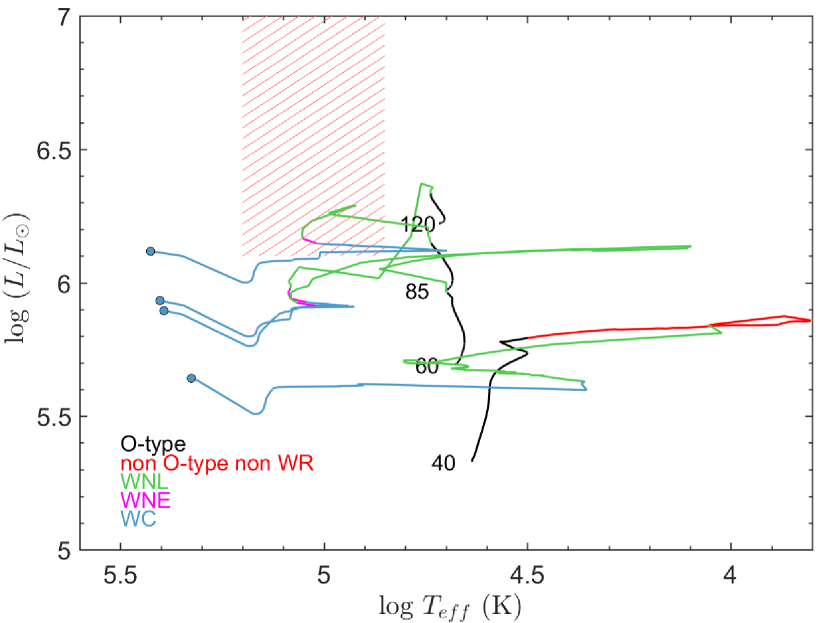
Figure 17: Hertzsprung-Russel diagram showing the locus of the progenitor of SN 2017ein. The evolutionary tracks of massive stars at solar metallicity from Georgy et al. (2012) are displayed for comparison. The numbers in the plot mark the corresponding ZAMS mass in unit of solar mass. The endpoints of the tracks are indicated by dots. Different colors on the lines represent different evolutionary stages of the stars.

7.3 Binary, star cluster and low ejecta mass

As an alternative, the high luminosity of the progenitor may be related to the contribution of a similarly luminous companion star. According to observations of WR stars in the Milky Way and Large Magellanic Cloud (LMC), one finds that more than 80% of luminous stars, i.e., M_V $<$ $-$5.5 mag, are found to be binaries, while this fraction drops to about 50% for the relatively faint counterparts (Hainich et al., 2014; van der Hucht, 2006). After examining the surrounding stars within a radius of 5 arc-seconds from the progenitor of SN 2017ein on the pre-explosion images, we find that the progenitor star does not stand out from them but clearly belongs to the relatively blue and luminous subgroup before subtracting host extinction, as shown in Figure 18. This, perhaps, favors a multi-system or star cluster as the source. In this case, we expect to see a bright star at the SN position when the supernova fades away in a few years.

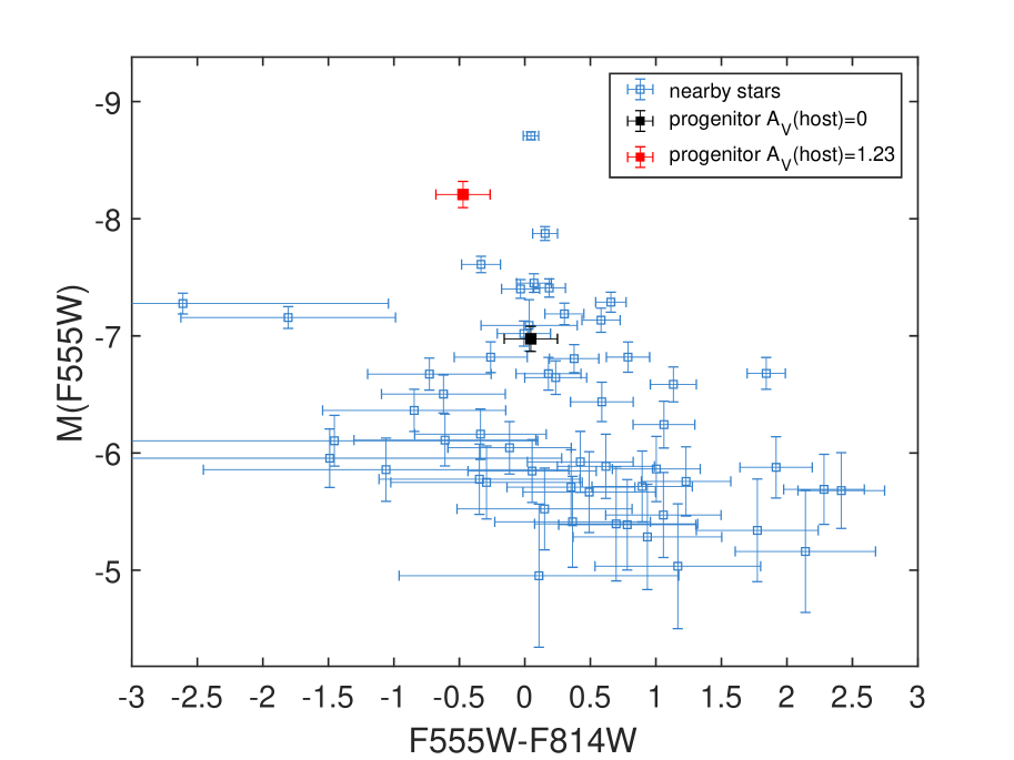
Figure 18: A color–absolute magnitude diagram of the progenitor candidate of SN 2017ein and its surrounding stars at a distance within 5 arcseconds. The absolute magnitudes and color index of the surrounding stars are corrected for Galactic extinction but not the host extinction. A distance modulus of $\mu=$31.38 mag is adopted.

Binary interaction can result in more efficient mass loss for massive stars, resulting in lower ejecta masses in supernovae. Lyman et al. (2016) found that explosions of stars with initial mass larger than $28$ M_⊙ will produce ejecta of mass not lower than 5 M_⊙, and even stars with initial mass $\geqslant$ 20 M_⊙ in binaries will produce ejecta of mass higher than 5 M_⊙. Thus, lower-mass binary models are in better agreement with the distribution of ejecta mass of SNe Ib/c. Considering the lower ejecta mass of $\sim$1 M_⊙ for SN 2017ein, it is more likely that its progenitor star is a lower mass star in a binary system rather than a single star with such a high initial mass. As discussed in Van Dyk et al. (2018), the progenitor is consistent with massive binary stars. Kilpatrick et al. (2018) has came to similar conclusions, prefering a binary model of 80$+$48 M_⊙. However, the expected ejecta mass is still higher than 5 M_⊙.

These results have demonstrated a connection between SN 2017ein and very massive progenitor stars, conflicting with the low ejecta mass. This may be related to mass loss in massive stars. The mass loss of massive stars dominates their evolution and determines their fate (Smith, 2014). However, the mass loss of massive stars is quite complicated. In addition to mass loss through strong and relatively mild stellar wind as WR stars, massive stars may experience eruptive mass loss, e.g. Luminous Blue Variables (LBVs). And some stars undergo explosive mass loss shortly (a few years) before explosion (Ofek et al., 2014; Gal-Yam et al., 2014; Yaron et al., 2017). Circumstellar dust can give rise to large uncertainty in observations of massive stars. Some WR systems reveal persistent or episodic dust formation within months or years, resulting in strong optical or IR variations with an amplitude of a few magnitudes of the WR binaries, due to the newly formatted dust or the asymmetry of the dust distribution (eg. Williams et al., 2009). This dust will eventually be ejected to the interstellar medium (ISM).

On the other hand, as also proposed by Van Dyk et al. (2018), the supernova explosion can also disrupt and vaporize circumstellar dust. These facts demonstrate that the extinction derived from the Na I D lines in the SN spectra, which mostly represent extinction from the interstellar dust, rather than the dust surrounding the star, can not be directly applied to the progenitor. The extinction to the SN should be a lower limit of the true extinction to the progenitor. As a result, the progenitor could be even bluer and brighter. Combining the effects of dust formation in massive stars and destruction by the SN explosion, the real extinction to the progenitor can be very complicated. Detailed discussions on the mass loss and dust formation and disruption in SN 2017ein is beyond the scope of this paper.

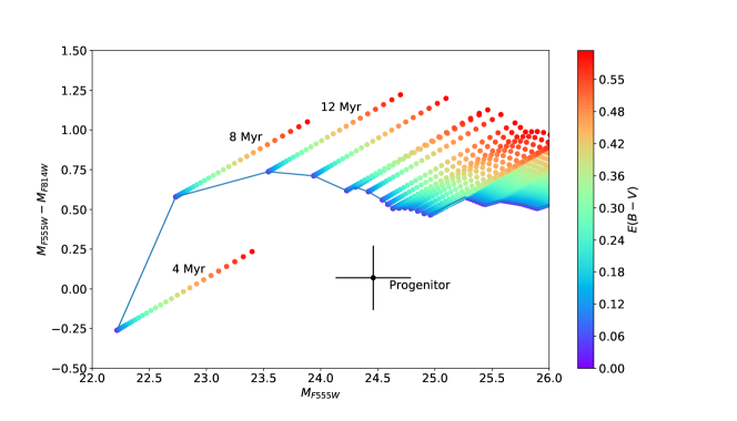
Figure 19: A set of cluster models from GALEV, for a $1\times 10^{4}$ M_⊙ cluster at solar metallicty. The color of each point denotes the assumed total reddening, while the line connects the $E(B-V)=0$ cluster models to guide the eye. All tracks have placed at the distance of SN 2017ein. The observed progenitor color and magnitude is indicated.

On the other hand, the progenitor candidate could also be a young and blue star cluster, as also pointed out by Van Dyk et al. (2018). As noted previously, a $\lesssim$16 pc cluster would be unresolved in the pre-explosion data. To explore this possibility, we created a set of models for a $10^{4}$ M_⊙ cluster with the GALEV code (Kotulla et al., 2009). We assume a single stellar population at solar metallicity, formed in a exponentially declining burst. In Figure 19, we compare the colour and magnitude of such a cluster to the source observed to be coincident with the SN. The relatively blue color of the source implies that the progenitor must be $\sim 4$ Myr old. The absolute magnitude of the observed source is much fainter than the model cluster, implying that it must be substantially less massive. Naively scaling our model magnitudes to the observed value, we find that the cluster would have a mass $\sim 2.5\times 10^{3}$ M_⊙. As a test of our results, we also compared to the colours of a set of BPASS models (v 2.2.1, Stanway & Eldridge, 2018), and found similar results.

Such a young cluster age implies that in this case the progenitor would have to be relatively massive. Taking the lifetimes of single massive stars from the STARS code (Eldridge et al., 2008), we find that the progenitor would of necessity have a zero age main sequence mass of $\gtrsim$40 M_⊙. Such a star would in fact lose its H envelope through stellar winds, and explode as a single WR star. For a Salpeter initial mass function between 0.1 and 300 M_⊙, and assuming a cluster of 2500 M_⊙, then only around 160 M_⊙ of the cluster mass will be in stars more massive than 40 M_⊙. So, if this were indeed the case, then the progenitor was one of the most massive members of the cluster.

The preceding analysis must be taken with considerable caution: with only two broadband filters it is extremely difficult to draw firm conclusions as to the properties of any possible cluster, especially when young clusters of hot massive stars will emit much of their flux at bluer wavelengths than F555W. We also caution that we cannot even be certain as to whether we are observing a single population – even a small 16 pc region could plausibly play host to multiple overlapping stellar populations. Future observations, and in particular in the UV, can help resolve this uncertainty.

8 Conclusions

We present the optical/ultraviolet observations of the nearby type Ic supernova SN 2017ein and analysis of the properties of the supernova and its progenitor, by taking advantages of both our extremely early-time photometry/spectroscopy and the public HST pre-explosion data. SN 2017ein is similar to SN 2007gr and SN 2013ge in overall spectral evolution, all characterized by prominent carbon features in the early phase, while SN 2017ein clearly shows some distinct features from the latter two. The expansion velocities of different lines of SN 2017ein are similar to the other two, but the Na I and Si II expansion velocities of SN 2017ein are higher than those of SN 2007gr, but comparable to those of SN 2013ge. Another interesting feature is that the absorption lines of the CaII NIR triplet split into two narrow lines at late phases, which was not seen in other SNe Ib/c including SNe 2007gr and 2013ge. This probably suggests that the line forming region of SN 2017ein is confined into a relatively narrow shell. Moreover, the late time light curves of SN 2017ein are fast declining, which is not seen in other SNe Ib/c.

From the very early photometry and non detection limit, we were able to constrain the first-light time of SN 2017ein to be within one day after explosion, representing one of the tightest constraints for SNe Ib/c. Most interestingly, the early data show a possible excess emission relative to the Ni decay model at one day after explosion, which can be attributed to the shock cooling tail. By fitting the $BVR$-band light curves, using a radioactive decay model and a shock cooling model, we find that the supernova synthesized ⁵⁶Ni mass of $\sim$0.13 M_⊙, and the stellar envelope has a radius of 8$\pm$4 R_⊙ and a mass of $\sim$0.02 M_⊙. Note that a smaller ejecta mass of $\sim$1 M_⊙ is found for SN 2017ein. This indicates that the progenitor star has lost most of its H/He envelope before collapse, consistent with a compact Wolf-Rayet star or a massive binary. SN 2017ein perhaps represents the first normal SN Ic observed to have a signature of shock breakout cooling from the stellar envelope. Undoubtedly, it provides a very good sample to test theories of SN Ic explosions.

By analyzing the pre-explosion HST images, we find a point-like source with an absolute magnitude of $M_{V}=-8.00\pm 0.34$ mag and $M_{I}=-7.53\pm 0.35$ mag coincides with the position of SN 2017ein. Assuming that the source is a single star, it is found to have an effective temperature of $\sim$70,800–159,000 K, a luminosity of $\mathrm{log}(L/L_{\odot})\gtrsim 6.1$, and a radius of $\sim$6–14 R_⊙, roughly consistent with a hot and luminous WR star. Comparing with stellar evolutionary tracks, we found that the initial mass of this star could exceed 60 M_⊙. Such a hot and luminous star is very rare and we did not find a similar star in current WR star catalogs. However, such massive star is inconsistent with the low ejecta mass found for SN 2017ein. On the other hand, it is also possible that the point source identified at the SN position could be a binary or a young, blue star cluster. The low ejecta mass inferred for SN 2017ein seems to favor for a low mass binary scenario. By comparing the observational data and SSP star cluster models at solar metallicity, we find that the source is consistent with star clusters with age of 4 Myr and a low mass of $\sim 2.5\times 10^{3}$ M_⊙. And the progenitor of SN 2017ein should be among the most massive members of the cluster. Due to the low resolution of the HST images and the lack of data in shorter wavelengths, it is difficult to decide which case is favored. Further distinguishing between different scenarios needs to wait for another visit of this galaxy with HST when the SN light dims out. SN 2017ein provides a rare opportunity that helps to throw light on massive star evolution and supernova explosion theories.

Table 7: Optical BVRI photometry of SN 2017ein.

MJD	B	V	R	I	Telescope
57904.605	16.438$\pm$0.026	15.885$\pm$0.013	15.571$\pm$0.030	15.245$\pm$0.017	TNT
57905.604	16.270$\pm$0.044	15.715$\pm$0.022	15.390$\pm$0.030	15.076$\pm$0.020	TNT
57906.598	16.083$\pm$0.026	15.506$\pm$0.016	15.208$\pm$0.032	14.912$\pm$0.021	TNT
57907.641	…	…	15.165$\pm$0.016	14.835$\pm$0.032	TNT
57908.574	15.929$\pm$0.028	15.347$\pm$0.014	15.057$\pm$0.029	14.735$\pm$0.015	TNT
57911.612	15.975$\pm$0.019	15.221$\pm$0.011	14.881$\pm$0.028	14.531$\pm$0.015	TNT
57912.592	16.038$\pm$0.022	15.209$\pm$0.012	14.852$\pm$0.030	14.496$\pm$0.014	TNT
57917.607	16.483$\pm$0.030	15.312$\pm$0.012	14.851$\pm$0.029	14.457$\pm$0.016	TNT
57919.573	16.644$\pm$0.029	15.436$\pm$0.016	14.928$\pm$0.033	14.490$\pm$0.016	TNT
57921.607	16.910$\pm$0.055	15.542$\pm$0.019	15.034$\pm$0.032	14.547$\pm$0.026	TNT
57930.549	17.678$\pm$0.035	16.280$\pm$0.018	15.626$\pm$0.037	14.982$\pm$0.020	TNT
57932.560	…	…	15.773$\pm$0.079	…	TNT
57933.566	…	16.591$\pm$0.134	15.855$\pm$0.053	15.258$\pm$0.071	TNT
57936.713	18.190$\pm$0.021	16.790$\pm$0.016	16.084$\pm$0.012	15.338$\pm$0.013	AZT
57937.712	18.184$\pm$0.026	16.804$\pm$0.016	16.127$\pm$0.008	…	AZT
57938.726	18.150$\pm$0.029	16.831$\pm$0.017	16.182$\pm$0.008	15.460$\pm$0.013	AZT
57940.694	18.334$\pm$0.047	16.921$\pm$0.020	16.257$\pm$0.010	15.512$\pm$0.019	AZT
57941.711	18.344$\pm$0.021	16.958$\pm$0.017	16.287$\pm$0.008	15.557$\pm$0.014	AZT
57942.723	18.325$\pm$0.040	16.944$\pm$0.023	16.330$\pm$0.010	15.562$\pm$0.013	AZT
57945.685	18.121$\pm$0.116	17.044$\pm$0.051	16.365$\pm$0.011	15.598$\pm$0.013	AZT
57946.721	18.606$\pm$0.110	17.001$\pm$0.022	16.364$\pm$0.011	15.600$\pm$0.013	AZT
57949.687	18.335$\pm$0.072	17.152$\pm$0.021	16.488$\pm$0.013	15.683$\pm$0.021	AZT
57950.695	18.556$\pm$0.028	17.093$\pm$0.017	16.503$\pm$0.011	15.678$\pm$0.014	AZT
57951.695	18.431$\pm$0.018	17.171$\pm$0.015	16.551$\pm$0.008	15.735$\pm$0.022	AZT
57952.684	18.500$\pm$0.094	17.210$\pm$0.020	16.544$\pm$0.012	15.732$\pm$0.019	AZT
57953.678	18.524$\pm$0.030	17.227$\pm$0.024	16.609$\pm$0.016	15.761$\pm$0.015	AZT
57954.686	18.600$\pm$0.018	17.239$\pm$0.019	16.621$\pm$0.015	15.788$\pm$0.018	AZT
57955.686	18.684$\pm$0.102	17.277$\pm$0.016	16.634$\pm$0.010	15.804$\pm$0.016	AZT
57956.693	18.800$\pm$0.120	17.269$\pm$0.026	16.615$\pm$0.017	15.796$\pm$0.017	AZT
57957.674	18.793$\pm$0.109	17.324$\pm$0.033	16.686$\pm$0.020	15.881$\pm$0.014	AZT
57958.683	18.715$\pm$0.049	17.338$\pm$0.024	16.715$\pm$0.009	15.888$\pm$0.013	AZT
57960.683	18.642$\pm$0.166	17.296$\pm$0.017	16.696$\pm$0.022	15.852$\pm$0.013	AZT
57963.670	18.460$\pm$0.039	17.449$\pm$0.046	16.786$\pm$0.011	15.908$\pm$0.016	AZT
57964.667	18.615$\pm$0.150	17.367$\pm$0.020	16.820$\pm$0.008	15.921$\pm$0.017	AZT
57965.667	18.820$\pm$0.028	17.410$\pm$0.034	16.827$\pm$0.015	15.969$\pm$0.016	AZT
58107.022	21.858$\pm$1.412	20.151$\pm$0.098	19.639$\pm$0.045	19.456$\pm$0.239	AZT
58124.882	21.636$\pm$1.494	22.635$\pm$1.440	19.852$\pm$0.108	21.230$\pm$1.004	AZT
58133.075	20.097$\pm$1.340	19.113$\pm$0.391	19.432$\pm$0.128	19.826$\pm$0.242	AZT
58139.040	20.039$\pm$0.322	22.644$\pm$1.036	21.158$\pm$0.104	20.422$\pm$0.098	AZT
58139.962	20.581$\pm$0.195	…	21.487$\pm$1.077	20.267$\pm$0.519	AZT
58140.954	…	21.599$\pm$0.905	21.372$\pm$1.064	20.900$\pm$0.605	AZT
58143.896	19.676$\pm$0.611	23.596$\pm$1.241	20.507$\pm$0.286	20.018$\pm$0.346	AZT
58150.919	20.158$\pm$1.441	21.834$\pm$0.605	19.399$\pm$0.246	21.078$\pm$0.933	AZT
58152.898	…	21.061$\pm$0.673	20.245$\pm$0.280	…	AZT
58154.958	21.784$\pm$0.727	21.371$\pm$0.196	20.674$\pm$0.194	…	AZT
58156.966	…	20.820$\pm$0.124	20.259$\pm$0.082	20.318$\pm$0.293	AZT
58167.949	20.121$\pm$0.756	20.633$\pm$0.149	21.456$\pm$0.336	19.844$\pm$0.425	AZT
58170.917	19.208$\pm$0.393	24.017$\pm$1.374	20.768$\pm$0.668	21.959$\pm$0.550	AZT
58171.904	20.520$\pm$0.840	21.682$\pm$0.310	21.252$\pm$0.136	20.347$\pm$0.227	AZT

Table 8: ATLAS photometry of SN 2017ein

MJD	AB mag	err	Filter	MJD	AB mag	err	Filter
57869.506	>20.06	1.35	c	57907.281	15.17	0.01	o
57869.520	>20.01	0.53	c	57907.296	15.16	0.01	o
57869.535	>19.87	2.18	c	57908.269	15.29	0.11	o
57869.550	>19.67	0.00	c	57908.284	15.25	0.05	o
57870.425	>20.13	0.00	c	57908.294	15.17	0.04	o
57870.437	>20.19	0.00	c	57911.261	14.84	0.01	o
57870.444	>20.21	0.45	c	57911.284	14.84	0.01	o
57870.459	>20.11	0.00	c	57911.300	14.84	0.01	o
57870.482	>20.12	0.56	c	57912.260	14.83	0.01	o
57882.354	>19.34	0.61	o	57912.262	14.84	0.01	o
57882.380	>19.52	0.00	o	57912.274	14.80	0.01	o
57882.391	>19.54	0.43	o	57912.291	14.79	0.01	o
57882.415	>19.44	2.92	o	57912.291	14.80	0.01	o
57887.280	>19.83	0.00	o	57912.304	14.85	0.01	o
57887.296	>19.80	0.73	o	57912.305	14.83	0.01	o
57887.307	>19.47	0.00	o	57914.269	14.93	0.01	o
57887.314	>19.64	0.00	o	57914.271	14.93	0.01	o
57887.320	>19.33	0.00	o	57914.290	14.88	0.01	o
57887.335	>19.59	0.97	o	57914.299	14.90	0.01	o
57887.339	>19.64	0.68	o	57914.302	14.92	0.01	o
57887.354	>19.62	1.02	o	57914.304	14.90	0.01	o
57892.322	>19.95	0.81	o	57914.318	14.94	0.01	o
57892.324	>19.72	0.00	o	57914.327	14.89	0.01	o
57892.337	>19.75	1.85	o	57914.335	14.91	0.01	o
57894.333	>20.24	0.00	c	57915.310	14.83	0.01	o
57894.356	>20.02	0.00	c	57915.333	14.81	0.01	o
57894.370	>20.09	0.97	c	57915.355	14.82	0.01	o
57894.390	>20.07	1.40	c	57918.269	14.86	0.01	o
57894.404	>20.11	0.00	c	57918.280	14.87	0.01	o
57896.252	>20.04	1.41	o	57922.260	15.00	0.01	o
57896.267	>20.07	0.00	o	57922.270	15.03	0.02	o
57896.283	>19.61	0.66	o	57925.250	15.15	0.01	o
57898.336	18.43	0.10	c	57925.260	15.16	0.01	o
57898.354	18.69	0.14	c	57925.278	15.17	0.01	o
57898.362	18.53	0.11	c	57925.283	15.15	0.01	o
57898.384	18.35	0.10	c	57927.278	15.38	0.01	o
57898.390	18.25	0.10	c	57927.287	15.40	0.01	o
57900.255	16.98	0.05	o	57929.259	15.55	0.01	o
57900.262	16.92	0.04	o	57929.262	15.53	0.01	o
57900.267	17.07	0.05	o	57929.277	15.52	0.01	o
57900.280	16.83	0.04	o	57929.286	15.52	0.01	o
57900.284	17.02	0.05	o	57933.259	15.75	0.01	o
57900.313	17.05	0.05	o	57933.262	15.80	0.02	o
57903.256	15.96	0.02	o	57933.276	15.74	0.01	o
57903.270	15.88	0.02	o	57933.287	15.79	0.02	o
57903.285	15.81	0.02	o	57937.258	16.00	0.02	o
57903.299	15.81	0.02	o	57937.263	16.01	0.02	o
57907.259	15.17	0.01	o	57937.273	16.04	0.02	o
57907.264	15.18	0.01	o	57937.288	16.03	0.02	o

Table 9: Swift-UVOT photometry of SN 2017ein.

MJD	uvw1	u	b	v
57900.510	…	17.619$\pm$0.213	17.943$\pm$0.182	17.133$\pm$0.181
57911.922	17.674$\pm$0.176	15.980$\pm$0.084	15.966$\pm$0.069	15.228$\pm$0.070
57915.465	17.713$\pm$0.189	16.812$\pm$0.123	16.188$\pm$0.075	15.221$\pm$0.072
57919.892	…	17.473$\pm$0.171	16.643$\pm$0.084	15.401$\pm$0.074
57923.103	…	18.238$\pm$0.288	17.094$\pm$0.099	15.737$\pm$0.080
57927.849	…	18.500$\pm$0.368	17.775$\pm$0.149	16.292$\pm$0.105
57933.992	…	…	18.114$\pm$0.224	16.764$\pm$0.162
57937.877	…	…	18.518$\pm$0.256	16.796$\pm$0.138
57942.460	…	…	18.409$\pm$0.240	16.928$\pm$0.154
57945.483	…	…	18.424$\pm$0.250	17.078$\pm$0.174
57949.869	…	…	18.382$\pm$0.346	16.699$\pm$0.196
57953.332	…	…	18.350$\pm$0.248	16.950$\pm$0.173
57955.423	…	…	18.253$\pm$0.205	17.057$\pm$0.161
57960.206	…	…	18.568$\pm$0.285	17.015$\pm$0.175

References

- Arcavi et al. (2017) Arcavi, I., Hosseinzadeh, G., Brown, P. J., et al. 2017, ApJ, 837, L2
- Arnett (1982) Arnett, W. D. 1982, Astrophysical Journal, 253, 785
- Asplund et al. (2009) Asplund, M., Grevesse, N., Sauval, A. J., & Scott, P. 2009, ARA&A, 47, 481
- Barbarino et al. (2017) Barbarino, C., Botticella, M. T., Dall’Ora, M., et al. 2017, MNRAS, 471, 2463
- Barbon et al. (1995) Barbon, R., Benetti, S., Cappellaro, E., et al. 1995, Astronomy and Astrophysics Supplement, 110, 513
- Berger et al. (2002) Berger, E., Kulkarni, S. R., & Chevalier, R. A. 2002, ApJ, 577, L5
- Bersten et al. (2014) Bersten, M. C., Benvenuto, O. G., Folatelli, G., et al. 2014, AJ, 148, 68
- Bersten et al. (2018) Bersten, M. C., Folatelli, G., Garc a, F., et al. 2018, Nature, 554, 497
- Bertin & Arnouts (1996) Bertin, E., & Arnouts, S. 1996, A&AS, 117, 393
- Bianco et al. (2014) Bianco, F. B., Modjaz, M., Hicken, M., et al. 2014, The Astrophysical Journal Supplement, 213, 19
- Breeveld et al. (2011) Breeveld, A. A., Landsman, W., Holland, S. T., et al. 2011, in American Institute of Physics Conference Series, Vol. 1358, American Institute of Physics Conference Series, ed. J. E. McEnery, J. L. Racusin, & N. Gehrels, 373–376
- Brown et al. (2014) Brown, P. J., Breeveld, A. A., Holland, S., Kuin, P., & Pritchard, T. 2014, Ap&SS, 354, 89
- Campana et al. (2006) Campana, S., Mangano, V., Blustin, A. J., et al. 2006, Nature, 442, 1008
- Cano (2014) Cano, Z. 2014, ApJ, 794, 121
- Cao et al. (2013) Cao, Y., Kasliwal, M. M., Arcavi, I., et al. 2013, ApJ, 775, L7
- Chen et al. (2014) Chen, J., Wang, X., Ganeshalingam, M., et al. 2014, Astrophysical Journal, 790, 120
- Clocchiatti et al. (1996) Clocchiatti, A., Wheeler, J. C., Brotherton, M. S., et al. 1996, Astrophysical Journal, 462, 462
- Corsi et al. (2011) Corsi, A., Ofek, E. O., Frail, D. A., et al. 2011, ApJ, 741, 76
- Crowther (2007) Crowther, P. A. 2007, Annual Review of Astronomy & Astrophysics, 45, 177
- Dessart et al. (2012) Dessart, L., Hillier, D. J., Li, C., & Woosley, S. 2012, MNRAS, 424, 2139
- Dolphin (2016) Dolphin, A. 2016, DOLPHOT: Stellar photometry, Astrophysics Source Code Library, , , ascl:1608.013
- Drout et al. (2011) Drout, M. R., Soderberg, A. M., Gal-Yam, A., et al. 2011, ApJ, 741, 97
- Drout et al. (2016) Drout, M. R., Milisavljevic, D., Parrent, J., et al. 2016, Astrophysical Journal, 821, 57
- Ehgamberdiev (2018) Ehgamberdiev, S. 2018, Nature Astronomy, 2, 349
- Ekström et al. (2012) Ekström, S., Georgy, C., Eggenberger, P., et al. 2012, A&A, 537, A146
- Eldridge et al. (2015) Eldridge, J. J., Fraser, M., Maund, J. R., & Smartt, S. J. 2015, MNRAS, 446, 2689
- Eldridge et al. (2013) Eldridge, J. J., Fraser, M., Smartt, S. J., Maund, J. R., & Crockett, R. M. 2013, MNRAS, 436, 774
- Eldridge et al. (2008) Eldridge, J. J., Izzard, R. G., & Tout, C. A. 2008, MNRAS, 384, 1109
- Eldridge & Maund (2016) Eldridge, J. J., & Maund, J. R. 2016, MNRAS, 461, L117
- Filippenko et al. (1995) Filippenko, A. V., Barth, A. J., Matheson, T., et al. 1995, Astrophysical Journal, 450, 11
- Foley et al. (2003) Foley, R. J., Papenkova, M. S., Swift, B. J., et al. 2003, The Publications of the Astronomical Society of the Pacific, 115, 1220
- Fox et al. (2014) Fox, O. D., Azalee Bostroem, K., Van Dyk, S. D., et al. 2014, ApJ, 790, 17
- Fremling et al. (2014) Fremling, C., Sollerman, J., Taddia, F., et al. 2014, A&A, 565, A114
- Fremling et al. (2018) Fremling, C., Sollerman, J., Kasliwal, M. M., et al. 2018, A&A, 618, A37
- Frey et al. (2013) Frey, L. H., Fryer, C. L., & Young, P. A. 2013, ApJ, 773, L7
- Gal-Yam et al. (2002) Gal-Yam, A., Ofek, E. O., & Shemmer, O. 2002, Monthly Notices of the Royal Astronomical Society, 332, L73
- Gal-Yam et al. (2014) Gal-Yam, A., Arcavi, I., Ofek, E. O., et al. 2014, Nature, 509, 471
- Galama et al. (1998) Galama, T. J., Vreeswijk, P. M., van Paradijs, J., et al. 1998, Nature, 395, 670
- Gehrels et al. (2004) Gehrels, N., Chincarini, G., Giommi, P., et al. 2004, ApJ, 611, 1005
- Georgy et al. (2012) Georgy, C., Ekström, S., Meynet, G., et al. 2012, Astronomy & Astrophysics, 332, A29
- Georgy et al. (2013) Georgy, C., Ekström, S., Eggenberger, P., et al. 2013, A&A, 558, A103
- Gordon et al. (2003) Gordon, K. D., Clayton, G. C., Misselt, K. A., Landolt, A. U., & Wolff, M. J. 2003, ApJ, 594, 279
- Groh et al. (2013) Groh, J. H., Georgy, C., & Ekström, S. 2013, A&A, 558, L1
- Guillochon et al. (2017) Guillochon, J., Parrent, J., Kelley, L. Z., & Margutti, R. 2017, ApJ, 835, 64
- Hachinger et al. (2012) Hachinger, S., Mazzali, P. A., Taubenberger, S., et al. 2012, MNRAS, 422, 70
- Hainich et al. (2014) Hainich, R., Rühling, U., Todt, H., et al. 2014, Astronomy & Astrophysics, 565, A27
- Hamuy & Pinto (2002) Hamuy, M., & Pinto, P. A. 2002, ApJ, 566, L63
- Heger et al. (2003) Heger, A., Fryer, C. L., Woosley, S. E., Langer, N., & Hartmann, D. H. 2003, Astrophysical Journal, 591, 288
- Huang et al. (2012) Huang, F., Li, J.-Z., Wang, X.-F., et al. 2012, Research in Astronomy and Astrophysics, 12, 1585
- Hunter et al. (2009) Hunter, D. J., Valenti, S., Kotak, R., et al. 2009, A&A, 508, 371
- Im et al. (2017) Im, M., Choi, C., Lee, S.-Y., et al. 2017, The Astronomer’s Telegram, 10481
- Iwamoto et al. (1998) Iwamoto, K., Mazzali, P. A., Nomoto, K., et al. 1998, Nature, 395, 672
- Iwamoto et al. (2000) Iwamoto, K., Nakamura, T., Nomoto, K., et al. 2000, ApJ, 534, 660
- Kaplan et al. (2016) Kaplan, K. F., Jogee, S., Kewley, L., et al. 2016, Monthly Notices of the Royal Astronomical Society, 462, 1642
- Kasen & Bildsten (2010) Kasen, D., & Bildsten, L. 2010, ApJ, 717, 245
- Kilpatrick et al. (2018) Kilpatrick, C. D., Takaro, T., Foley, R. J., et al. 2018, MNRAS, 480, 2072
- Kotulla et al. (2009) Kotulla, R., Fritze, U., Weilbacher, P., & Anders, P. 2009, MNRAS, 396, 462
- Li et al. (2014) Li, X., Hjorth, J., & Wojtak, R. 2014, ApJ, 796, L4
- Liu et al. (2016) Liu, Y.-Q., Modjaz, M., Bianco, F. B., & Graur, O. 2016, ApJ, 827, 90
- Lyman et al. (2016) Lyman, J. D., Bersier, D., James, P. A., et al. 2016, MNRAS, 457, 328
- Magnier et al. (2016) Magnier, E. A., Schlafly, E. F., Finkbeiner, D. P., et al. 2016, ArXiv e-prints, arXiv:1612.05242
- Maund et al. (2004) Maund, J. R., Smartt, S. J., Kudritzki, R. P., Podsiadlowski, P., & Gilmore, G. F. 2004, Nature, 427, 129
- Mazzali et al. (2008) Mazzali, P. A., Valenti, S., Della Valle, M., et al. 2008, Science, 437, 1185
- Meynet & Maeder (2003) Meynet, G., & Maeder, A. 2003, Astronomy & Astrophysics, 404, 975
- Modjaz et al. (2011) Modjaz, M., Kewley, L., Bloom, J. S., et al. 2011, ApJ, 731, L4
- Modjaz et al. (2008) Modjaz, M., Kewley, L., Kirshner, R. P., et al. 2008, AJ, 135, 1136
- Modjaz et al. (2009) Modjaz, M., Li, W., Butler, N., et al. 2009, The Astronomical Journal, 702, 226
- Modjaz et al. (2014) Modjaz, M., Blondin, S., Kirshner, R. P., et al. 2014, The Astronomical Journal, 147, 99
- Nakamura et al. (2001) Nakamura, T., Mazzali, P. A., Nomoto, K., & Iwamoto, K. 2001, ApJ, 550, 991
- Nicholl et al. (2017) Nicholl, M., Guillochon, J., & Berger, E. 2017, ApJ, 850, 55
- Ofek et al. (2014) Ofek, E. O., Sullivan, M., Shaviv, N. J., et al. 2014, ApJ, 789, 104
- Patat et al. (2001) Patat, F., Cappellaro, E., Danziger, J., et al. 2001, Astrophysical Journal, 555, 900
- Paxton et al. (2015) Paxton, B., Marchant, P., Schwab, J., et al. 2015, ApJS, 220, 15
- Piro (2015) Piro, A. L. 2015, Astrophysical Journal, 808, L51
- Piro & Nakar (2013) Piro, A. L., & Nakar, E. 2013, ApJ, 769, 67
- Podsiadlowski et al. (1993) Podsiadlowski, P., Hsu, J. J. L., Joss, P. C., & Ross, R. R. 1993, Nature, 364, 509
- Poole et al. (2008) Poole, T. S., Breeveld, A. A., Page, M. J., et al. 2008, MNRAS, 383, 627
- Poznanski et al. (2009) Poznanski, D., Butler, N., Filippenko, A. V., et al. 2009, ApJ, 694, 1067
- Prentice & Mazzali (2017) Prentice, S. J., & Mazzali, P. A. 2017, MNRAS, 469, 2672
- Prentice et al. (2018) Prentice, S. J., Ashall, C., Mazzali, P. A., et al. 2018, MNRAS, 478, 4162
- Richmond et al. (1996) Richmond, M. W., van Dyk, S. D., Ho, W., et al. 1996, The Astronomical Journal, 111, 327
- Rodríguez et al. (2014) Rodríguez, Ó., Clocchiatti, A., & Hamuy, M. 2014, AJ, 148, 107
- Roming et al. (2005) Roming, P. W. A., Kennedy, T. E., Mason, K. O., et al. 2005, Space Sci. Rev., 120, 95
- Sander et al. (2012) Sander, A., Hamann, W.-R., & Todt, H. 2012, Astronomy & Astrophysics, 540, A144
- Schlafly & Finkbeiner (2011) Schlafly, E. F., & Finkbeiner, D. P. 2011, The Astrophysical Journal, 737, 103
- Smartt (2015) Smartt, S. J. 2015, Publications of the Astronomical Society of Australia, 32, 16
- Smartt et al. (2009) Smartt, S. J., Eldridge, J. J., Crockett, R. M., & Maund, J. R. 2009, MNRAS, 395, 1409
- Smith & Maeder (1991) Smith, L. F., & Maeder, A. 1991, Astronomy & Astrophysics, 241, 77
- Smith (2014) Smith, N. 2014, ARA&A, 52, 487
- Stanway & Eldridge (2018) Stanway, E. R., & Eldridge, J. J. 2018, MNRAS, 479, 75
- Taddia et al. (2016) Taddia, F., Fremling, C., Sollerman, J., et al. 2016, A&A, 592, A89
- Taubenberger et al. (2006) Taubenberger, S., Pastorello, A., Mazzali, P. A., et al. 2006, MNRAS, 371, 1459
- Thomas et al. (2011) Thomas, R. C., Nugent, P. E., & Meza, J. C. 2011, PASP, 123, 237
- Tody (1986) Tody, D. 1986, in Proc. SPIE, Vol. 627, Instrumentation in astronomy VI, ed. D. L. Crawford, 733
- Tody (1993) Tody, D. 1993, in Astronomical Society of the Pacific Conference Series, Vol. 52, Astronomical Data Analysis Software and Systems II, ed. R. J. Hanisch, R. J. V. Brissenden, & J. Barnes, 173
- Tonry et al. (2018) Tonry, J. L., Denneau, L., Heinze, A. N., et al. 2018, PASP, 130, 064505
- Tully (1988) Tully, R. B. 1988, Nearby galaxies catalog
- Turatto et al. (2003) Turatto, M., Benetti, S., & Cappellaro, E. 2003, in From Twilight to Highlight: The Physics of Supernovae, 200
- Valenti et al. (2008) Valenti, S., Elias-Rosa, N., Taubenberger, S., et al. 2008, The Astrophysical Journal Letters, 673, L155
- van der Hucht (2006) van der Hucht, K. A. 2006, A&A, 458, 453
- Van Dyk et al. (2018) Van Dyk, S. D., Zheng, W., Brink, T. G., et al. 2018, ApJ, 860, 90
- Wang et al. (2016) Wang, L.-J., Wang, S. Q., Dai, Z. G., et al. 2016, The Astrophysical Journal, 821, 22
- Wang et al. (2017) Wang, L. J., Yu, H., Liu, L. D., et al. 2017, The Astrophysical Journal, 837, 128
- Waxman & Katz (2016) Waxman, E., & Katz, B. 2016, ArXiv e-prints, arXiv:1607.01293
- Waxman et al. (2007) Waxman, E., Mésázros, P., & Campana, S. 2007, The Astrophysical Journal, 667, 351
- Williams et al. (2009) Williams, P. M., Marchenko, S. V., Marston, A. P., et al. 2009, MNRAS, 395, 1749
- Xiang et al. (2017) Xiang, D., Song, H., Wang, X., et al. 2017, The Astronomer’s Telegram, 10434
- Yamanaka et al. (2017) Yamanaka, M., Nakaoka, T., Tanaka, M., et al. 2017, ApJ, 837, 1
- Yaron et al. (2017) Yaron, O., Perley, D. A., Gal-Yam, A., et al. 2017, Nature Physics, 13, 510
- Yokoo et al. (1994) Yokoo, T., Arimoto, J., Matsumoto, K., Takahashi, A., & Sadakane, K. 1994, PASJ, 46, L191
- Yoon et al. (2018) Yoon, S.-C., Chun, W., Tolstov, A., Blinnikov, S., & Dessart, L. 2018, ArXiv e-prints, arXiv:1810.03108