Intersection cuts for factorable MINLP

Abstract

Given a factorable function $f$, we propose a procedure that constructs a concave underestimor of $f$ that is tight at a given point. These underestimators can be used to generate intersection cuts. A peculiarity of these underestimators is that they do not rely on a bounded domain. We propose a strengthening procedure for the intersection cuts that exploits the bounds of the domain. Finally, we propose an extension of monoidal strengthening to take advantage of the integrality of the non-basic variables.

Keywords: Mixed-integer nonlinear programming, intersection cuts, monoidal strengthening.

1 Introduction

In this work we propose a procedure for generating intersection cuts for mixed integer nonlinear programs (MINLP). We consider MINLP of the following form

$$\max c^{\mathsf{T}}x$$ (1)

 s.t. $$g_{j}(x)\leq 0,j\in J$$

$$Ax=b$$

$$x_{i}\in\mathbb{Z},i\in I$$

$$x\geq 0,$$

where $J=\{1,\ldots,l\}$ denotes the indices of the nonlinear constraints, $g_{j}\colon\mathbb{R}^{n}\to\mathbb{R}$ are assumed to be continuous and factorable (see Definition 1), $A\in\mathbb{R}^{m\times n}$, $c\in\mathbb{R}^{n}$, $b\in\mathbb{R}^{m}$, and $I\subseteq\{1,\ldots,n\}$ are the indices of the integer variables. We denote the set of feasible solutions by $S$ and a generic relaxation of $S$ by $R$, that is, $S\subseteq R$. When $R$ is a translated simplicial cone and $C$ contains its apex and no point of $S$ in its interior, valid inequalities for $\operatorname{conv}(R\setminus C)$ are called intersection cuts [2]. See the excellent survey [18] for recent developments and details on intersection cuts for mixed integer linear programs (MILP).

Many applications can be modeled as MINLP [13]. The current state of the art for solving MINLP to global optimality is via linear programming (LP), convex nonlinear programming and (MILP) relaxations of $S$, together with spatial branch and bound [10, 25, 26, 28, 37, 40]. Roughly speaking, the LP-based spatial branch and bound algorithm works as follows. The initial polyhedral relaxation is solved and yields $\bar{x}$. If the solution $\bar{x}$ is feasible for (1), we obtain an optimal solution. If not, we try to separate the solution from the feasible region. This is usually done by considering each violated constraint separately. Let $g(x)\leq 0$ be a violated constraint of (1). If $g(\bar{x})>0$ and $g$ is convex, then $g(\bar{x})+v^{\mathsf{T}}(x-\bar{x})\leq 0$, where $v\in\partial g(\bar{x})$ and $\partial g(\bar{x})$ is the subdifferential of $g$ at $\bar{x}$, is a valid cut. If $g_{j}$ is non-convex, then a convex underestimator $g_{vex}$, that is, a convex function such that $g_{vex}(x)\leq g(x)$ over the feasible region, is constructed and if $g_{vex}(\bar{x})>0$ the previous cut is constructed for $g_{vex}$. If the point cannot be separated, then we branch, that is, we select a variable $x_{k}$ in a violated constraint and split the problem into two problems, one with $x_{k}\leq\bar{x}_{k}$ and the other one with $x_{k}\geq\bar{x}_{k}$.

Applying the previous procedure to the MILP case, that is (1) with $J=\emptyset$, reveals a problem with this approach. In this case, the polyhedral relaxation is just the linear programming (LP) relaxation. Assuming that $\bar{x}$ is not feasible for the MILP, then there is an $i\in I$ such that $x_{i}\notin\mathbb{Z}$. Let us treat the constraint $x_{i}\in\mathbb{Z}$ as a nonlinear non-convex constraint represented by some function as $g(x_{i})\leq 0$. Then, $g(\bar{x}_{i})>0$. However, a convex underestimator $\bar{g}$ of $g$ must satisfy that $g_{vex}(z)\leq 0$ for every $z\in\mathbb{R}$, since $g_{vex}(z)\leq g(z)\leq 0$ for every $z\in\mathbb{Z}$ and $g_{vex}(z)$ is convex. Since separation is not possible, we need to branch.

However, for the current state-of-the-art algorithms for MILP, cutting planes are a fundamental component [1]. A classical technique for building cutting planes in MILP is based on exploiting information from the simplex tableau [18]. When solving the LP relaxation, we obtain $x_{B}=\bar{x}_{B}+Rx_{N}$, where $B$ and $N$ are the indices of the basic and non-basic variables, respectively. Since $\bar{x}$ is infeasible for the MILP, there must be some $k\in B\cap I$ such that $\bar{x}_{k}\notin\mathbb{Z}$. Now, even though $\bar{x}$ cannot be separated from the violated constraint $x_{k}\in\mathbb{Z}$, the equivalent constraint, $\bar{x}_{k}+\sum_{j\in N}r_{kj}x_{j}\in\mathbb{Z}$ can be used to separate $\bar{x}$.

In the MINLP case, this framework generates equivalent non-linear constraints with some appealing properties. The change of variables $x_{k}=\bar{x}_{k}+\sum_{j\in N}r_{kj}x_{j}$ for the basic variables present in a violated nonlinear constraint $g(x)\leq 0$, produces the non-linear constraint $h(x_{N})\leq 0$ for which $h(0)>0$ and $x_{N}\geq 0$. Assuming that the convex envelope of $h$ exists in $x_{N}\geq 0$, then we can always construct a valid inequality. Indeed, by [36, Corollary 3], the convex envelope of $h$ is tight at 0. Since an $\epsilon$-subgradient always exists for any $\epsilon>0$ and $x\in\operatorname{dom}h$ [14], an $\frac{h(0)}{2}$-subgradient, for instance, at 0 will separate it.

Even when there is no convex underestimator for $h$, a valid cutting plane does exist. Continuity of $h$ implies that $X=\{x_{N}\geq 0:h(x_{N})\leq 0\}$ is closed and [17, Lemma 2.1] ensures that $0\notin\overline{conv}X$, thus, a valid inequality exists. We introduce a technique to construct such a valid inequality. The idea is to build a concave underestimator of $h$, ${h}_{ave}$, such that ${h}_{ave}(0)=h(0)>0$. Then, $C=\{x_{N}:{h}_{ave}(x_{N})\geq 0\}$ is an $S$-free set, that is, a convex set that does not contain any feasible point in its interior, and as such can be used to build an intersection cut (IC) [39, 2, 21].

First contribution

In Section 3, we present a procedure to build concave underestimators for factorable functions that are tight at a given point. The procedure is similar to McCormick’s method for constructing convex underestimators, and generalizes Proposition 3.2 and improves Proposition 3.3 of [24]. These underestimators can be used to build intersection cuts. We note that IC from a concave underestimator can generate cuts that cannot be generated by using the convex envelope. This should not be surprising, given that intersection cuts work at the feasible region level, while convex underestimators depend on the graph of the function. A simple example is $\{x\in[0,2]:-x^{2}+1\leq 0\}$. When separating 0, the intersection cut gives $x\geq 1$, while using the convex envelope over $[0,2]$ yields $x\geq 1/2$.

There are many differences between concave underestimators and convex ones. Maybe the most interesting one is that concave underestimators do not need bounded domains to exist. As an extreme example, $-x^{2}$ is a concave underestimator of itself, but a convex underestimator only exists if the domain of $x$ is bounded. Even though this might be regarded as an advantage, it is also a problem. If concave underestimators are independent of the domain, then we cannot improve them when the domain shrinks.

Second contribution

In Section 4, we propose a strengthening procedure that uses the bounds of the variables to enlarge the $S$-free set. Our procedure improves on the one used by Tuy [39].

Other techniques for strengthening IC have been proposed, such as, exploiting the integrality of the non-basic variables [5, 19, 20], improving the relaxation $R$ [6, 30, 31] and computing the convex hull of $R\setminus C$ [8, 17, 22, 34, 35].

Third contribution

By interpreting IC as disjunctive cuts [3], we extend monoidal strengthening to our setting [5] in Section 5. Although its applicability seems to be limited, we think it is of independent interest, specially for MILP.

2 Related work

There have been many efforts on generalizing cutting planes from MILP to MINLP, we refer the reader to [29] and the references therein. In [29], the authors study how to compute $\operatorname{conv}(R\setminus C)$ where $R$ is not polyhedral, but $C$ is a $k$-branch split. In practice, such sets $C$ usually come from the integrality of the variables. Works that build sets $C$ which do not come from integrality considerations include [9, 11, 33, 32]. We refer to [12] and the references therein for more details. We would like to point out that the disjunctions built in [9, 33, 32] can be interpreted as piecewise linear concave underestimators. However, our approach is not suitable for disjunctive cuts built through cut generating LPs [4], since we generate infinite disjunctions, see Section 5, so we rely on the classical concept of intersection cuts where $R$ is a translated simplicial cone.

Khamisov [24] studies functions $f:\mathbb{R}^{n}\to\mathbb{R}$, representable as $f(x)=\max_{y\in R}\varphi(x,y)$ where $\varphi$ is continuous and concave on $x$. These functions allow for a concave underestimator at every point. He shows that this class of functions is very general, in particular, the class of functions representable as difference of convex functions is a strict subset of this class. He then shows how to build concave underestimators of some functions. The technique in [24] for building an underestimator for the composition of two functions is a special case of Theorem 4 below, and the one for building an underestimator for the product requires a compact domain. We simplify the construction for the product and no longer need a compact domain.

Although not directly related to this work, other papers that use underestimators other than convex are [15, 16, 23].

3 Concave underestimators

In his seminal paper [27], McCormick proposed a method to build convex underestimators of factorable functions.

Definition 1.

Given a set of univariate functions $\mathcal{L}$, e.g.,$\mathcal{L}=\{\cos,\cdot^{n},\exp,\log,\text{...}\}$, the set of factorable functions $\mathcal{F}$ is the smallest set that contains $\mathcal{L}$, the constant functions, and is closed under addition, product and composition.

As an example, $e^{-(\cos(x^{2})+xy/4)^{2}}$ is a factorable function for $\mathcal{L}=\{\cos,\exp\}$.

Given the inductive definition of factorable functions, to show a property about them one just needs to show that said property holds for all the functions in $\mathcal{L}$, constant functions, and that it is preserved by the product, addition and composition. For instance, McCormick [27] proves, constructively, that every factorable function admits a convex underestimator and a concave overestimator, by showing how to construct estimators for the sum, product and composition of two functions for which estimators are known.

An estimator for the sum of two functions is the sum of the estimators. For the product, McCormick uses the well-known McCormick inequalities. Less known is the way McCormick handles the composition $f(g(x))$. Let $f_{vex}$ be a convex underestimator of $f$ and $z_{\min}=\operatorname{arg\,min}f_{vex}(z)$. Let $g_{vex}$ be a convex underestimator of $g$ and $g^{ave}$ a concave overestimator. McCormick shows that $f_{vex}(\operatorname{mid}\{g_{vex}(x),g^{ave}(x),z_{\min}\})$ is a convex underestimator of $f(g(x))$, where $\operatorname{mid}\{x,y,z\}$ is the median between $x,y$ and $z$. It is well known that the optimum of a convex function over a closed interval is given by such a formula, thus

$$f_{vex}(\operatorname{mid}\{g_{vex}(x),g^{ave}(x),z_{\min}\})=\min\{f_{vex}(z):z\in[g_{vex}(x),g^{ave}(x)]\},$$

see also [38].

Definition 2.

Let $\mathcal{X}\subseteq\mathbb{R}^{n}$ be convex, and $f:\mathcal{X}\to\mathbb{R}$ be a function. We say that $f_{ave}:\mathcal{X}\to\mathbb{R}$ is a concave underestimator of $f$ at $\bar{x}\in\mathcal{X}$ if $f_{ave}(x)$ is concave, $f_{ave}(x)\leq f(x)$ for every $x\in\mathcal{X}$ and $f_{ave}(\bar{x})=f(\bar{x})$. Similarly we define a convex overestimator of $f$ at $\bar{x}\in\mathcal{X}$.

Remark 3.

For simplicity, we will consider only the case where $\mathcal{X}=\mathbb{R}^{n}$. This restriction leaves out some common functions like $\log$. One possibility to include these function is to let the range of the function to be $\mathbb{R}\cup\{\pm\infty\}$. Then, $\log(x)=-\infty$ for $x\in\mathbb{R}_{-}$. Note that other functions like $\sqrt{x}$ can be handled by replacing them by a concave underestimator defined on all $\mathbb{R}$.

We now show that every factorable function admits a concave underestimator at a given point. Since the case for the addition is easy, we just need to specify how to build concave underestimators and convex overestimators for

• the product of two functions for which estimators are known,

• the composition $f(g(x))$ where estimators of $f$ and $g$ are known and $f$ is univariate.

Theorem 4.

Let $f:\mathbb{R}\to\mathbb{R}$ and $g:\mathbb{R}^{n}\to\mathbb{R}$. Let $g_{ave},f_{ave}$ be, respectively, a concave underestimator of $g$ at $\bar{x}$ and of $f$ at $g(\bar{x})$. Further, let $g^{vex}$ a convex overestimator of $g$ at $\bar{x}$. Then,

$$h(x):=\min\{f_{ave}(g_{ave}(x)),f_{ave}(g^{vex}(x))\},$$

is a concave underestimator of $f(g(x))$ at $\bar{x}$.

Proof.

Clearly, $h(\bar{x})=f(g(\bar{x}))$.

To establish $h(x)\leq f(g(x))$, notice that

$$h(x)=\min\{f_{ave}(z):g_{ave}(x)\leq z\leq g^{vex}(x)\}.$$ (2)

Since $z=g(x)$ is a feasible solution and $f_{ave}$ is an underestimator of $f$, we obtain that $h(x)\leq f(g(x))$.

Now, let us prove that $h$ is concave. To this end, we again use the representation (2). To simplify notation, we write $g_{1},g_{2}$ for $g_{ave},g^{vex}$, respectively.
We prove concavity by definition, that is,

$$h(\lambda x_{1}+(1-\lambda)x_{2})\geq\lambda h(x_{1})+(1-\lambda)h(x_{2}),\text{ for }\lambda\in[0,1].$$

Let

$$I =[g_{1}(\lambda x_{1}+(1-\lambda)x_{2}),g_{2}(\lambda x_{1}+(1-\lambda)x_{2})]$$

$$J =[\lambda g_{1}(x_{1})+(1-\lambda)g_{1}(x_{2}),\lambda g_{2}(x_{1})+(1-\lambda)g_{2}(x_{2})].$$

By the concavity of $g_{1}$ and convexity of $g_{2}$ we have $I\subseteq J$. Therefore,

$$h(\lambda x_{1}+(1-\lambda)x_{2})=\min\{f_{ave}(z):z\in I\}\geq\min\{f_{ave}(z):z\in J\}.$$

Since $f_{ave}$ is concave, the minimum is achieved at the boundary,

$$\min\{f_{ave}(z):z\in J\}=\min_{i\in\{1,2\}}f_{ave}(\lambda g_{i}(x_{1})+(1-\lambda)g_{i}(x_{2})).$$

Furthermore, $f_{ave}(\lambda g_{i}(x_{1})+(1-\lambda)g_{i}(x_{2}))\geq\lambda f_{ave}(g_{i}(x_{1}))+(1-\lambda)f_{ave}(g_{i}(x_{2}))$ which implies that

$$h(\lambda x_{1}+(1-\lambda)x_{2}) \geq\min_{i\in\{1,2\}}\lambda f_{ave}(g_{i}(x_{1}))+(1-\lambda)f_{ave}(g_{i}(x_{2}))$$

$$\geq\min_{i\in\{1,2\}}\lambda f_{ave}(g_{i}(x_{1}))+\min_{i\in\{1,2\}}(1-\lambda)f_{ave}(g_{i}(x_{2}))$$

$$=\lambda h(x_{1})+(1-\lambda)h(x_{2}),$$

as we wanted to show. ∎

Remark 5.

The generalization of Theorem 4 to the case where $f$ is multivariate in the spirit of [38] is straightforward.

The computation of a concave underestimator and convex overestimator of the product of two functions reduces to the computation of estimators for the square of a function through the polarization identity

$$4f(x)g(x)=(f(x)+g(x))^{2}-(f(x)-g(x))^{2}.$$

Let $h:\mathbb{R}^{n}\to\mathbb{R}$ for which we know estimators $h_{vex}\leq h\leq h^{ave}$ at $\bar{x}$. From Theorem 4, a convex overestimator of $h^{2}$ at $\bar{x}$ is given by $\max\{{h_{vex}}^{2},{h^{ave}}^{2}\}$. On the other hand, a concave underestimator of $h^{2}$ at $\bar{x}$ can be constructed from the underestimator $h^{2}(x)\geq h^{2}(\bar{x})+2h(\bar{x})(h(x)-h(\bar{x}))$. From here we obtain

$$\begin{cases}2h(\bar{x})h^{ave}(x)-h^{2}(\bar{x}),&\text{ if }h(\bar{x})\leq 0\\ 2h(\bar{x})h_{vex}(x)-h^{2}(\bar{x}),&\text{ if }h(\bar{x})>0.\end{cases}$$ (3)

Example 1.

Let us compute a concave underestimator of $f(x)=e^{-(\cos(x^{2})+x/4)^{2}}$ at $0$. Estimators of $x^{2}$ are given by $0\leq x^{2}\leq x^{2}$. For $\cos(x)$, estimators are $\cos(x)-x^{2}/2\leq\cos(x)\leq 1$. Then, a concave underestimator of $\cos(x^{2})$ is, according to Theorem 4, $\min\{\cos(0)-0^{2}/2,\cos(x^{2})-x^{4}/2\}=\cos(x^{2})-x^{4}/2$. A convex overestimator is 1. Hence, $\cos(x^{2})-x^{4}/2+x/4\leq\cos(x^{2})+x/4\leq 1+x/4$.

Given that $-x^{2}$ is concave, a concave underestimator of $-(\cos(x^{2})+x/4)^{2}$ is $\min\{-(\cos(x^{2})-x^{4}/2+x/4)^{2},-(1+x/4)^{2}\}$. To compute a convex overestimator of $-(\cos(x^{2})+x/4)^{2}$, we compute a concave underestimator of $(\cos(x^{2})+x/4)^{2}$. Since, $\cos(x^{2})+x/4$ at 0 is $1$, (3) yields $2(\cos(x^{2})-x^{4}/2+x/4)-1$.

Finally, a concave underestimator of $e^{x}$ at $x=-1$ is just its linearization, $e^{-1}+e^{-1}(x+1)$ and so $e^{-1}+e^{-1}(1+\min\{-(\cos(x^{2})-x^{4}/2+x/4)^{2},-(1+x/4)^{2}\})$ is a concave underestimator of $f(x)$. The intermediate estimators as well as the final concave underestimator are illustrated in Figure 1.

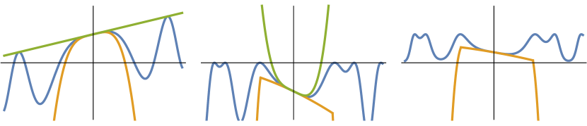
Figure 1: Concave underestimator (orange) and convex overestimator (green) of $\cos(x^{2})+x/4$ (left), $-(\cos(x^{2})+x/4)^{2}$ (middle) and $f(x)$ (right) at $x=0$.

∎

For ease of exposition, in the rest of the paper we assume that the concave underestimator is differentiable. All results can be extended to the case where the functions are only sub- or super-differentiable.

4 Enlarging the $S$-free sets by using bound information

In Section 3, we showed how to build concave underestimators which give us $S$-free sets. Note that the construction does not make use of the bounds of the domain. We can exploit the bounds of the domain by the observation that the concave underestimator only needs to underestimate within the feasible region. However, to preserve the convexity of the $S$-free set, we must ensure that the underestimator is still concave.

Let $h(x)\leq 0$ be a constraint of (1), assume $x\in[l,u]$ and let $h_{ave}$ be a concave underestimator of $h$. Throughout this section, $S=\{x\in[l,u]:h(x)\leq 0\}$. In order to construct a concave function $\hat{h}$ such that $\{x:\hat{h}(x)\geq 0\}$ contains $\{x:h_{ave}(x)\geq 0\}$, consider the following function

$$\hat{h}(x)=\min\{h_{ave}(z)+\nabla h_{ave}(z)^{\mathsf{T}}(x-z):\ z\in[l,u],\ h_{ave}(z)\geq 0\}.$$ (4)

A similar function was already considered by Tuy [39]. The only difference is that Tuy’s strengthening does not use the restriction $h_{ave}(z)\geq 0$, see Figure 2.

Proposition 6.

Let $h_{ave}$ be a concave underestimator of $h$ at $\bar{x}\in[l,u]$, such that $h(\bar{x})>0$. Define $\hat{h}$ as in (4). Then, the set $C=\{x:\hat{h}(x)\geq 0\}$ is a convex $S$-free set and $C\supseteq\{x:h_{ave}(x)\geq 0\}$.

Proof.

The function $\hat{h}$ is concave since it is the minimum of linear functions. This establishes the convexity of $C$.

To show that $C\supseteq\{x:h_{ave}(x)\geq 0\}$, notice that $h_{ave}(x)=\min_{z}h_{ave}(z)+\nabla h_{ave}(z)^{\mathsf{T}}(x-z)$. The inclusion follows from observing that the objective function in the definition of $\hat{h}(x)$ is the same as above, but over a smaller domain.

To show that it is $S$-free, we will show that for every $x\in[l,u]$ such that $h(x)\leq 0$, $\hat{h}(x)\leq 0$.

Let $x_{0}\in[l,u]$ such that $h(x_{0})\leq 0$. Since $h_{ave}$ is a concave underestimator at $\bar{x}$, $h_{ave}(\bar{x})>0$ and $h_{ave}(x_{0})\leq 0$. If $h_{ave}(x_{0})=0$, then, by definition, $\hat{h}(x_{0})\leq h_{ave}(x_{0})=0$ and we are done. We assume, therefore, that $h_{ave}(x_{0})<0$.

Consider $g(\lambda)=h_{ave}(\bar{x}+\lambda(x_{0}-\bar{x}))$ and let $\lambda_{1}\in(0,1)$ be such that $g(\lambda_{1})=0$. The existence of $\lambda_{1}$ is justified by the continuity of $g$, $g(0)>0$ and $g(1)<0$. Equivalently, $x_{1}=\bar{x}+\lambda_{1}(x_{0}-\bar{x})$ is the intersection point between the segment joining $x_{0}$ with $\bar{x}$ and $\{x:h_{ave}(x)=0\}$. The linearization of $g$ at $\lambda_{1}$ evaluated at $\lambda=1$ is negative, because $g$ is concave, and equals $h_{ave}(x_{1})+\nabla h_{ave}(x_{1})^{T}(x_{0}-x_{1})$. Finally, given that $x_{1}\in[l,u]$ and $h_{ave}(x_{1})=0$, $x_{1}$ is feasible for (4) and we conclude that $\hat{h}(x_{0})<0$. ∎

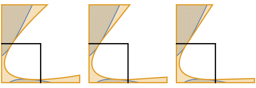
Figure 2: Feasible region $\{x,y\in[0,2]:h(x,y)\leq 0\}$, where $h=x^{2}-2y^{2}+4xy-3x+2y+1$, in blue together with $h_{ave}(x,y)\leq 0$ at $\bar{x}=(1,1)$ (left), Tuy’s strengthening (middle) and $\hat{h}\leq 0$ (right) in orange. Region shown is $[0,4]^{2}$, $[0,2]^{2}$ is bounded by black lines.

5 “Monoidal” strengthening

We show how to strengthen cuts from reverse convex constraints when exactly one non-basic variable is integer. Our technique is based on monoidal strengthening applied to disjunctive cuts, see Lemma 8 and the discussion following it. If more than one variable is integer, we can generate one cut per integer variable, relaxing the integrality of all but one variable at a time. However, under some conditions (see Remark 11), we can exploit the integrality of several variables at the same time. Our exposition of the monoidal strengthening technique is slightly different from [5] and is inspired by [41, Section 4.2.3].

Throughout this section, we assume that we already have a concave underestimator, and that we have performed the change of variables described in the introduction. Therefore, we consider the constraint $\{x\in[0,u]:h(x)\leq 0\}$ where $h:\mathbb{R}^{n}\to\mathbb{R}$ is concave and $h(0)>0$. Let $Y=\{y\in[0,u]:h(y)=0\}$. The convex $S$-free set $C=\{x\in[0,u]:h(x)\geq 0\}$ can be written as

$$C =\bigcap_{y\in Y}\{x\in[0,u]:\nabla h(y)^{\mathsf{T}}x\geq\nabla h(y)^{\mathsf{T}}y\}.$$

The concavity of $h$ implies that $h(0)\leq h(y)-\nabla h(y)^{\mathsf{T}}y$ for all $y$ in the domain of $h$. In particular, if $y\in Y$, then $\nabla h(y)^{\mathsf{T}}y\leq-h(0)<0$. Since all feasible points satisfy $h(x)\leq 0$, they must satisfy the infinite disjunction

$$\bigvee_{y\in Y}\frac{\nabla h(y)^{\mathsf{T}}}{\nabla h(y)^{\mathsf{T}}y}x\geq 1.$$ (5)

The maximum principle [3] implies that with

$$\alpha_{j}=\max_{y\in Y}\frac{\partial_{j}h(y)}{\nabla h(y)^{\mathsf{T}}y},$$ (6)

the cut $\sum_{j}\alpha_{j}x_{j}\geq 1$ is valid. We remark that the maximum exists, since the concavity of $h$ implies that for $y\in Y$, $h(e_{j})\leq\partial_{j}h(y)-\nabla h(y)^{\mathsf{T}}y$. This implies, together with $\nabla h(y)^{\mathsf{T}}y\leq-h(0)<0$, that $\tfrac{\partial_{j}h(y)}{\nabla h(y)^{\mathsf{T}}y}\leq 1+\tfrac{h(e_{j})}{\nabla h(y)^{\mathsf{T}}y}$. If $h(e_{j})\geq 0$, then $\tfrac{\partial_{j}h(y)}{\nabla h(y)^{\mathsf{T}}y}\leq 1$. Otherwise, $\tfrac{\partial_{j}h(y)}{\nabla h(y)^{\mathsf{T}}y}\leq 1-\tfrac{h(e_{j})}{h(0)}$.

The application of monoidal strengthening [5, Theorem 3] to a valid disjunction $\bigvee_{i}\alpha^{i}x\geq 1$ requires the existence of bounds $\beta_{i}$ such that $\alpha^{i}x\geq\beta$ is valid for every feasible point. Let $\beta(y)$ be such a bound for (5). An example of $\beta(y)$ is

$$\beta(y)=\min_{x\in[0,u]}\frac{\nabla h(y)^{\mathsf{T}}x}{\nabla h(y)^{\mathsf{T}}y}.$$

Remark 7.

If $\beta(y)\geq 1$, then $\nabla h(y)^{\mathsf{T}}x/\nabla h(y)^{\mathsf{T}}y\geq 1$ is redundant and can be removed from (5). Therefore, we can assume without loss of generality that $\beta(y)<1$.

The strengthening derives from the fact that a new disjunction can be obtained from (5) and, with it, a new disjunctive cut. The disjunction on the following Lemma is trivially satisfied, but provides the basis for building non-trivial new disjunctions.

Lemma 8.

Every $x\geq 0$ that satisfies (5), also satisfies

$$\bigvee_{y\in Y}\frac{\nabla h(y)^{\mathsf{T}}x}{\nabla h(y)^{\mathsf{T}}y}+z(y)(1-\beta(y))\geq 1,$$ (7)

where $z\colon Y\to\mathbb{Z}$ is such that $z\equiv 0$ or there is a $y_{0}\in Y$ for which $z(y_{0})>0$.

Proof.

If $z\equiv 0$, then (7) reduces to (5).

Otherwise, let $y_{0}\in Y$ such that $z(y_{0})>0$, that is, $z(y_{0})\geq 1$. By Remark 7, for every $y\in Y$, it holds $1-\beta(y)>0$, and so

$$z(y_{0})(1-\beta(y_{0}))\geq 1-\beta(y_{0}).$$

Therefore, $\beta(y_{0})\geq 1-z(y_{0})(1-\beta(y_{0}))$. Since every $x\geq 0$ satisfying (5) satisfies $\frac{\nabla h(y_{0})^{\mathsf{T}}x}{\nabla h(y_{0})^{\mathsf{T}}y_{0}}\geq\beta(y_{0})$, we conclude that $\frac{\nabla h(y_{0})^{\mathsf{T}}x}{\nabla h(y_{0})^{\mathsf{T}}y_{0}}+z(y_{0})(1-\beta(y_{0}))\geq 1$ holds. ∎

Remark 9.

Even if some disjunctive terms have no lower bound, that is, $\beta(y)=-\infty$ for $y\in Y^{\prime}\subseteq Y$, Lemma 8 still holds if, additionally, $z(y)=0$ for all $y\in Y^{\prime}$. This means that we are not using that disjunction for the strengthening. In particular, if for some variable $x_{j}$, $\alpha_{j}$ is defined by some $y\in Y^{\prime}$, then this cut coefficient cannot be improved.

Assume now that $x_{k}\in\mathbb{Z}$ for every $k\in K\subseteq\{1,\ldots,n\}$. To construct a new disjunction, we need to find a set of functions $M$ such that for any choice of $m^{k}\in M$ and any feasible assignment of $x_{k}$, $\sum_{k\in K}x_{k}m^{k}(y)$ satisfies the conditions of Lemma 8, that is, it must be in

$$Z=\{z\colon Y\to\mathbb{Z}:z\equiv 0\vee\exists y\in Y,z(y)>0\}.$$

Once such a family of functions has been identified, the cut $\sum_{j}\gamma_{j}x_{j}\geq 1$ with $\gamma_{j}=\alpha_{j}$ if $j\notin K$, and

$$\gamma_{k}=\inf_{m\in M}\max_{y\in Y}\frac{\partial_{k}h(y)}{\nabla h(y)^{\mathsf{T}}y}+m(y)(1-\beta(y))\quad\text{for }k\in K,$$ (8)

is valid and at least as strong as (6). Any $M\subseteq Z$ such that $(M,+)$ is a monoid, that is, $0\in M$ and $M$ is closed under addition can be used in (8).

Remark 10.

This is exactly what is happening in [5, Theorem 3]. Indeed, in the finite case, that is, when $Y$ is finite, Balas and Jeroslow considered $M=\{m\in\mathbb{Z}^{Y}:\sum_{y\in Y}m_{y}\geq 0\}$. Clearly, $(M,+)$ is a monoid and $M\subseteq Z$. Therefore, Lemma 8 implies that $\bigvee_{y\in Y}\alpha^{y}x+\sum_{k}m^{k}_{y}x_{k}(1-\beta_{y})\geq 1$ is valid for any choice of $m^{k}\in M$, which in turn implies [5, Theorem 3].
For an application that uses a different monoid see [7].

The question that remains is how to choose $M$. For example, the monoid $M=\{m\colon Y\to\mathbb{Z}:m\text{ has finite support and }\sum_{y\in Y}m(y)\geq 0\}$ is an obvious candidate for $M$. However, the problem is how to optimize over such an $M$, see (8).

We circumvent this problem by considering only one integer variable at a time. Fix $k\in K$. In this setting we can use $Z$ as $M$, which is not a monoid. Indeed, if $z\in Z$, then $x_{k}z\in Z$ for any $x_{k}\in\mathbb{Z}_{+}$. The advantage of using $Z$ is that the solution of (8) is easy to characterize.

With $M=Z$, the cut coefficients (8) of all variables are the same as (6) except for $x_{k}$. The cut coefficient of $x_{k}$ is given by

$$\inf_{z\in Z}\max_{y\in Y}\frac{\partial_{k}h(y)}{\nabla h(y)^{\mathsf{T}}y}+z(y)(1-\beta(y)).$$

To compute this coefficient, observe that one would like to have $z(y)<0$ for points $y$ such that the objective function of (6) is large. However, $z$ must be positive for at least one point. Therefore,

$$\min_{y\in Y}\frac{\partial_{k}h(y)}{\nabla h(y)^{\mathsf{T}}y}+(1-\beta(y))$$

is the best coefficient we can hope for if $z\not\equiv 0$. This coefficient can be achieved by

$$z(y)=\begin{cases}1,&\text{ if }y\in\operatorname{arg\,min}_{y\in Y}\frac{\partial_{k}h(y)}{\nabla h(y)^{\mathsf{T}}y}+(1-\beta(y)),\\ -L,&\text{ otherwise }\end{cases}$$ (9)

where $L>0$ is sufficiently large.

Summarizing, we can obtain the following cut:

$$\alpha_{j}=\begin{cases}\max_{y\in Y}\frac{\partial_{j}h(y)}{\nabla h(y)^{\mathsf{T}}y}&\text{ if }j\neq k\\ \min\{\max_{y\in Y}\frac{\partial_{j}h(y)}{\nabla h(y)^{\mathsf{T}}y},\min_{y\in Y}\frac{\partial_{j}h(y)}{\nabla h(y)^{\mathsf{T}}y}+(1-\beta(y))\}&\text{ if }j=k\end{cases}$$ (10)

Remark 11.

Let $z^{k}\in Z$ be given by (9) for each $k\in K$. Assume there is a subset $K_{0}\subseteq K$ and a monoid $M\subseteq Z$ such that $z^{k}\in M$ for every $k\in K_{0}$. Then, the strengthening can be applied to all $x_{k}$ for $k\in K_{0}$.

Alternatively, if there is a constraint enforcing that at most one of the $x_{k}$ can be non-zero for $k\in K_{0}$, e.g., $\sum_{k\in K}x_{k}\leq 1$, then the strengthening can be applied to all $x_{k}$ for $k\in K_{0}$.

Example 2.

Consider the constraint $\{x\in\{0,1,2\}\times[0,5]:h(x)\leq 0\}$, where $h(x_{1},x_{2})=-10x_{1}^{2}-1/2x_{2}^{2}+2x_{1}x_{2}+4$, see Figure 3. The IC is given by $\sqrt{5/2}x_{1}+1/(2\sqrt{2})x_{2}\geq 1$. Note that $(1/\sqrt{10},\sqrt{10})\in Y$ and yields the term $1/\sqrt{10}x_{2}\geq 1$ in (5). Since $x_{2}\geq 0$, $\beta(1/\sqrt{10},\sqrt{10})=0$. Hence, (10) yields $\alpha_{1}\leq\min\{\sqrt{5/2},1\}=1$ and the strengthened inequality is $x_{1}+1/(2\sqrt{2})x_{2}\geq 1$.

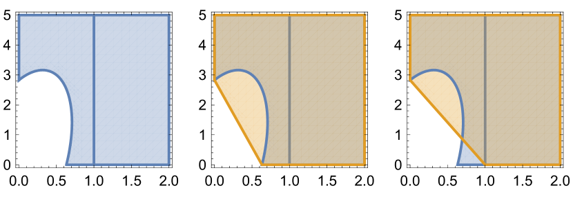
Figure 3: The feasible region $\{x\in\{0,1,2\}\times[0,5]:h(x)\leq 0\}$ from 2 (left), the IC (middle), and the strengthened cut (right).

∎

6 Conclusions

We have introduced a procedure to generate concave underestimators of factorable functions, which can be used to generate intersection cuts, together with two strengthening procedures.

It remains to be seen the practical performance of these intersection cuts. We expect that its generation is cheaper than the generation of disjunctive cuts, given that there is no need to solve an LP. As for the strengthening procedures, they might be too expensive to be of practical use. An alternative is to construct a polyhedral inner approximation of the $S$-free set and use monoidal strengthening in the finite setting. However, in this case, the strengthening proposed in Section 4 has no effect. Nonetheless, as far as the author knows, this has been the first application of monoidal strengthening that is able to exploit further problem structure such as demonstrated in Remark 11 and it might be interesting to investigate further.

Acknowledgments

The author is indebted to Stefan Vigerske and Franziska Schlösser for many helpful discussions and comments that improved the manuscript. He would also like to thank Sven Wiese, Ambros Gleixner, Dan Steffy and Juan Pablo Vielma for helpful discussions, and Leon Eifler, Daniel Rehfeldt for comments that improved the manuscript.

References

- [1] T. Achterberg and R. Wunderling. Mixed integer programming: Analyzing 12 years of progress. In Facets of Combinatorial Optimization, pages 449–481. Springer Berlin Heidelberg, 2013.
- [2] E. Balas. Intersection cuts—a new type of cutting planes for integer programming. Operations Research, 19(1):19–39, feb 1971.
- [3] E. Balas. Disjunctive programming. In Discrete Optimization II, Proceedings of the Advanced Research Institute on Discrete Optimization and Systems Applications of the Systems Science Panel of NATO and of the Discrete Optimization Symposium co-sponsored by IBM Canada and SIAM Banff, Aha. and Vancouver, pages 3–51. Elsevier BV, 1979.
- [4] E. Balas, S. Ceria, and G. Cornuéjols. A lift-and-project cutting plane algorithm for mixed 0–1 programs. Mathematical Programming, 58(1-3):295–324, jan 1993.
- [5] E. Balas and R. G. Jeroslow. Strengthening cuts for mixed integer programs. European Journal of Operational Research, 4(4):224–234, apr 1980.
- [6] E. Balas and F. Margot. Generalized intersection cuts and a new cut generating paradigm. Mathematical Programming, 137(1-2):19–35, aug 2011.
- [7] E. Balas and A. Qualizza. Monoidal cut strengthening revisited. Discrete Optimization, 9(1):40–49, feb 2012.
- [8] A. Basu, G. Cornuéjols, and G. Zambelli. Convex sets and minimal sublinear functions. Journal of Convex Analysis, 18(2):427–432, 2011.
- [9] P. Belotti. Disjunctive cuts for nonconvex MINLP. In Mixed Integer Nonlinear Programming, pages 117–144. Springer New York, nov 2011.
- [10] P. Belotti, J. Lee, L. Liberti, F. Margot, and A. W chter. Branching and bounds tightening techniques for non-convex MINLP. Optimization Methods and Software, 24(4-5):597–634, oct 2009.
- [11] D. Bienstock, C. Chen, and G. Muñoz. Outer-product-free sets for polynomial optimization and oracle-based cuts.
- [12] P. Bonami, J. Linderoth, and A. Lodi. Disjunctive cuts for mixed integer nonlinear programming problems. Progress in Combinatorial Optimization, pages 521–541, 2011.
- [13] F. Boukouvala, R. Misener, and C. A. Floudas. Global optimization advances in mixed-integer nonlinear programming, MINLP, and constrained derivative-free optimization, CDFO. European Journal of Operational Research, 252(3):701–727, aug 2016.
- [14] A. Brondsted and R. T. Rockafellar. On the subdifferentiability of convex functions. Proceedings of the American Mathematical Society, 16(4):605, aug 1965.
- [15] C. Buchheim and C. D’Ambrosio. Monomial-wise optimal separable underestimators for mixed-integer polynomial optimization. Journal of Global Optimization, 67(4):759–786, may 2016.
- [16] C. Buchheim and E. Traversi. Separable non-convex underestimators for binary quadratic programming. In Experimental Algorithms, pages 236–247. Springer Berlin Heidelberg, 2013.
- [17] M. Conforti, G. Cornuéjols, A. Daniilidis, C. Lemaréchal, and J. Malick. Cut-generating functions and S-free sets. Mathematics of Operations Research, 40(2):276–391, may 2015.
- [18] M. Conforti, G. Cornuéjols, and G. Zambelli. Corner polyhedron and intersection cuts. Surveys in Operations Research and Management Science, 16(2):105–120, jul 2011.
- [19] M. Conforti, G. Cornuéjols, and G. Zambelli. A geometric perspective on lifting. Operations Research, 59(3):569–577, jun 2011.
- [20] S. S. Dey and L. A. Wolsey. Two row mixed-integer cuts via lifting. Mathematical Programming, 124(1-2):143–174, may 2010.
- [21] F. Glover. Convexity cuts and cut search. Operations Research, 21(1):123–134, feb 1973.
- [22] F. Glover. Polyhedral convexity cuts and negative edge extensions. Zeitschrift f r Operations Research, 18(5):181–186, oct 1974.
- [23] M. M. F. Hasan. An edge-concave underestimator for the global optimization of twice-differentiable nonconvex problems. Journal of Global Optimization, 71(4):735–752, mar 2018.
- [24] O. Khamisov. On optimization properties of functions, with a concave minorant. Journal of Global Optimization, 14(1):79–101, 1999.
- [25] M. R. Kılınç and N. V. Sahinidis. Exploiting integrality in the global optimization of mixed-integer nonlinear programming problems with BARON. Optimization Methods and Software, 33(3):540–562, jul 2017.
- [26] Y. Lin and L. Schrage. The global solver in the LINDO API. Optimization Methods and Software, 24(4-5):657–668, oct 2009.
- [27] G. P. McCormick. Computability of global solutions to factorable nonconvex programs: Part i — convex underestimating problems. Mathematical Programming, 10(1):147–175, dec 1976.
- [28] R. Misener and C. A. Floudas. ANTIGONE: Algorithms for coNTinuous / Integer Global Optimization of Nonlinear Equations. Journal of Global Optimization, 59(2-3):503–526, mar 2014.
- [29] S. Modaresi, M. R. Kılınç, and J. P. Vielma. Intersection cuts for nonlinear integer programming: convexification techniques for structured sets. Mathematical Programming, 155(1-2):575–611, feb 2015.
- [30] M. Porembski. How to extend the concept of convexity cuts to derive deeper cutting planes. Journal of Global Optimization, 15(4):371–404, 1999.
- [31] M. Porembski. Finitely convergent cutting planes for concave minimization. Journal of Global Optimization, 20(2):109–132, 2001.
- [32] A. Saxena, P. Bonami, and J. Lee. Convex relaxations of non-convex mixed integer quadratically constrained programs: extended formulations. Mathematical Programming, 124(1-2):383–411, may 2010.
- [33] A. Saxena, P. Bonami, and J. Lee. Convex relaxations of non-convex mixed integer quadratically constrained programs: projected formulations. Mathematical Programming, 130(2):359–413, mar 2010.
- [34] S. Sen and H. D. Sherali. Facet inequalities from simple disjunctions in cutting plane theory. Mathematical Programming, 34(1):72–83, jan 1986.
- [35] S. Sen and H. D. Sherali. Nondifferentiable reverse convex programs and facetial convexity cuts via a disjunctive characterization. Mathematical Programming, 37(2):169–183, jun 1987.
- [36] M. Tawarmalani and N. V. Sahinidis. Convex extensions and envelopes of lower semi-continuous functions. Mathematical Programming, 93(2):247–263, dec 2002.
- [37] M. Tawarmalani and N. V. Sahinidis. A polyhedral branch-and-cut approach to global optimization. Mathematical Programming, 103(2):225–249, may 2005.
- [38] A. Tsoukalas and A. Mitsos. Multivariate McCormick relaxations. Journal of Global Optimization, 59(2-3):633–662, apr 2014.
- [39] H. Tuy. Concave programming with linear constraints. In Doklady Akademii Nauk, volume 159, pages 32–35. Russian Academy of Sciences, 1964.
- [40] S. Vigerske and A. Gleixner. SCIP: global optimization of mixed-integer nonlinear programs in a branch-and-cut framework. Optimization Methods and Software, 33(3):563–593, jun 2017.
- [41] S. Wiese. On the interplay of Mixed Integer Linear, Mixed Integer Nonlinear and Constraint Programming. PhD thesis, 2016.