Design of a Networked Controller for a Two-Wheeled Inverted Pendulum Robot

Abstract

The topic of this paper is to use an intuitive model-based approach to design a networked controller for a recent benchmark scenario. The benchmark problem is to remotely control a two-wheeled inverted pendulum robot via W-LAN communication. The robot has to keep a vertical upright position. Incorporating wireless communication in the control loop introduces multiple uncertainties and affects system performance and stability. The proposed networked control scheme employs model predictive techniques and deliberately extends delays in order to make them constant and deterministic. The performance of the resulting networked control system is evaluated experimentally with a predefined benchmarking experiment and is compared to local control involving no delays.

otherfnsymbols•∘§§‡‡‖∥¶¶

reset** ‡‡

1 Introduction

Advancements in communication and computation technology have led to the concept of Networked Control Systems (NCSs), cf. Hespanha et al. (2007). In an NCS, components are distributed and interact via a communication network. This allows a considerable increase in flexibility, but also raises many design challenges (Bemporad et al. (2010),Walsh et al. (2002)). In the case of wireless communication, non-deterministic delays and packet losses are characteristic phenomena. Delays are traditionally assumed shorter than the sampling time, see Nilsson et al. (1998), or compensated by adopting a Model Predictive Control scheme as in Mori et al. (2014). On the other hand, packet loss is commonly compensated by either employing H-infinity control design, see Ishii (2008), or gain-scheduling feedback, see Yu et al. (2008). A variety of further methods and approaches have been proposed to address these challenges (cf. Zhang et al. (2016)).

The purpose of this paper is to design a networked controller for a recently proposed benchmark problem. The benchmark, described in detail in Zoppi et al. (2019) and Gallenmüller et al. (2018), is to remotely control a two-wheeled inverted pendulum robot (TWIPR) over a wireless network, see Fig. 1. To make the benchmark inexpensive and easily reproducible, the widespread platform LEGO Mindstorm EV3 is used to realize the robot. All details regarding plant and controller are publicly accessible at https://github.com/tum-lkn/iccps-release.

Figure 1: Networked Control of a TWIPR. In Section 4.1, the asymmetry in wireless data transmission (dotted and unbroken lines) will be explained.

The body of the robot is mounted on two wheels, on which two DC motors are splined. The control objective is to keep the robot in a vertical upright position while undergoing a predefined benchmarking experiment. To the best of our knowledge, the design of a networked controller for a TWIPR has not been addressed yet. Among other authors, Pathak et al. (2005) stabilized a TWIPR using local, i.e., non-networked, control. Ananyevskiy and Fradkov (2017) proposed a control strategy over internet for coordinating oscillations of a group of pendula and validated it experimentally using LEGO Mindstorm NXT. Synchronization was not always achieved, and the controller did not compensate for lost communication packets.

In the current paper we design a networked controller for a TWIPR by using two previously suggested strategies (cf. Hespanha et al. (2007)): (i) we deliberately extend the actuation delays of the NCS in order to make them constant and deterministic; (ii) a sequence of future control inputs is computed from a sequence of model-based state predictions and is sent to the robot via the wireless network. If a control packet is lost, the robot uses the last received sequence of control inputs and applies the input corresponding to the current instant.

The remainder of this paper is organized as follows: in Section 2, a discrete-time linear dynamical plant model is presented and the available sensor information is described. Section 4 introduces a local controller that is used as a baseline for the networked controller developed in Section 4. The performance of both controllers is compared in Section 5.

In the following, the set of nonnegative (positive) integers is $\mathbb{N}_{0}$ ($\mathbb{N}$). The set of real numbers is $\mathbb{R}$. The set of nonnegative (positive) real numbers is denoted $\mathbb{R}_{\geq 0}$ ($\mathbb{R}_{>0}$). Given a time-dependent real-valued signal $x:\mathbb{R}_{\geq 0}\mapsto\mathbb{R}$, its first and second derivative with respect to time are denoted $\dot{x}$ and $\ddot{x}$. Given a vector $\bm{v}\in\mathbb{R}^{n}$, $n\in\mathbb{N}$, its transpose is $\bm{v}^{\prime}$, while the element in position $i\in\{1,\dots,n\}$ is $\bm{v}_{i}$. Given a matrix $A\in\mathbb{R}^{n\times m}$, its i-th column, with $i\in\{1,\dots,m\}$, is $[A]_{i}$.

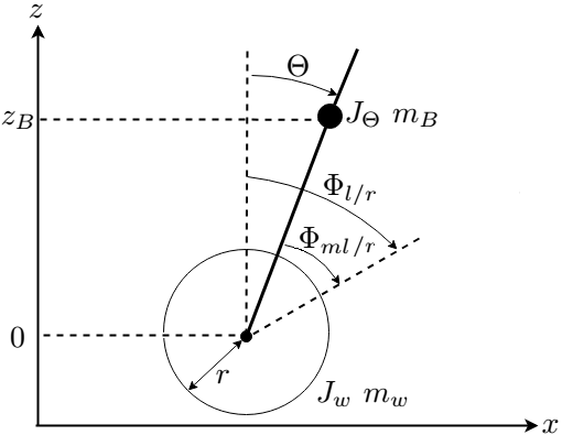
(a) Side view

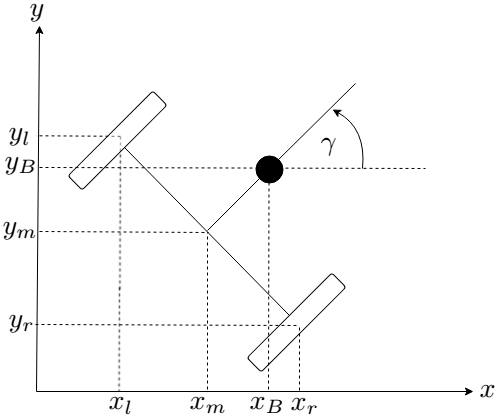
(b) Top view

Figure 2: Idealized mechanical model of the TWIPR.

2 Problem Description

Symbol	Unit	Description
$\Theta$	rad	Body pitch angle
$\Phi_{r}(\Phi_{l})$	rad	Rotation angle of the right (left) wheel
$\Phi_{mr}(\Phi_{ml})$	rad	Rotation angle of the right (left) motor
$\Phi:=\frac{(\Phi_{r}+\Phi_{l})}{2}$	rad	Average rotation angle of the wheels
$\gamma$	rad	Yaw angle of the body

Table 1: Kinematic Variables

2.1 Dynamical Model

Fig. 2 sketches the robot from the side and the top views and illustrates the sign convention; the depicted kinematic variables are given in Table 1. Throughout this section, the focus is not on the derivation of a dynamic model for the system, since this has been exhaustively addressed elsewhere, e.g. the nonlinear dynamic model of a TWIPR can be found in (Kim et al., 2005, pg. 33). With the model of the TWIPR at hand (Kim et al., 2005, pg. 33), let

$${\bm{x}}(t)=[\Phi(t),\Theta(t),\dot{\Phi}(t),\dot{\Theta}(t),\gamma(t),\dot{\gamma}(t)]^{\prime},$$ (1)

be the state vector and ${\bm{u}}(t)=[u_{l}(t),u_{r}(t)]^{\prime}$ the input, where $u_{l}(t)$ ($u_{r}(t)$) is the voltage applied to the left (right) DC-motor at time $t$. The nonlinear continuous-time model is

$$\forall t\in\mathbb{R}_{\geq 0},\text{ }\dot{{\bm{x}}}(t)=f({\bm{x}}(t),{\bm{u}}(t)),$$ (2)

and the linearized continuous-time dynamics (around the origin) is

$$\dot{\bm{x}}(t)=A{\bm{x}}(t)+B{\bm{u}}(t).$$ (3)

Matrices $A\in\mathbb{R}^{6\times 6}$ and $B\in\mathbb{R}^{6\times 2}$ are given in (Kim et al., 2005, pg. 38). Since sensors and controller are implemented based on a digital scheme, the system is discretized using the Forward Euler Method with a discretization step $T_{s}\in\mathbb{R}_{>0}$, which yields the discrete-time linear system, $\forall k\in\mathbb{N}_{0}$,

$${\bm{x}}_{d}(k+1)=A_{d}{\bm{x}}_{d}(k)+B_{d}{\bm{u}}_{d}(k),$$ (4)

where $A_{d}\in\mathbb{R}^{6\times 6}$, $B_{d}\in\mathbb{R}^{6\times 2}$ and

$${\bm{x}}_{d}(k)={\bm{x}}(kT_{s}),\quad{\bm{u}}_{d}(k)={\bm{u}}(kT_{s}),\quad\forall k\in\mathbb{N}_{0}.$$

Finally, for the specific hardware under consideration, a backlash occurs between each motor shaft and the respective wheel (see Nordin et al. (1997)), which is not captured by the model. We define a nonlinear function $\bm{f}_{\mathrm{bl}}:\mathbb{R}^{2}\mapsto\mathbb{R}^{2}$ to model the impact of the backlash on the input to the motors. Then, (4) is rewritten as

$${\bm{x}}_{d}(k+1)=A_{d}{\bm{x}}_{d}(k)+B_{d}\bm{f}_{\mathrm{bl}}({\bm{u}}_{d}(k)).$$ (5)

Further details are in (Nordin et al., 1997, pg. 55).

2.2 Sensors and Measurements

The robot is equipped with a single-axis digital gyroscope (mounted on the body) measuring the body pitch rate. Two digital encoders are splined on the two motor shafts and measure the left and the right motor angles. Let, $\forall k\in\mathbb{N}_{0},\ \dot{\Theta}^{(m)}(k)$ be the measurement coming from the gyroscope, and let $b(k)$ be the measurement bias of that gyroscope, which is determined from quasi-static measurements using standard bias estimation approaches, see Tin Leung et al. (2011). Finally, let $k\in\mathbb{N}_{0},\Phi_{ml}^{(m)}(k),\Phi_{mr}^{(m)}(k)$ be the left and right encoder measurements, respectively.

The states of system (4) can be estimated as follows:

$$\forall k\in\mathbb{N}_{0},\quad {\dot{\Theta}}(k)=\dot{\Theta}^{(m)}(k)-b(k),$$ (6)

$${\Theta}(k)={\Theta}(k-1)+T_{s}{\dot{\Theta}}(k),$$ (7)

$${\Phi}(k)=\frac{\Phi_{ml}^{(m)}(k)+\Phi_{mr}^{(m)}(k)}{2}+{\Theta}(k),$$ (8)

$${\dot{\Phi}}(k)=\frac{{\Phi}(k)-{\Phi}(k-1)}{T_{s}},$$ (9)

$${\gamma}(k)=\frac{r}{W}(\Phi_{mr}^{(m)}(k)-\Phi_{ml}^{(m)}(k)),$$ (10)

$${\dot{\gamma}}(k)=\frac{{\gamma}(k)-{\gamma}(k-1)}{T_{s}},$$ (11)

where ${\Theta}(0)=\Theta_{0}\in\mathbb{R}$, ${\rho}(0)=0$, ${\Phi}(0)=0$, and ${\gamma}(0)=0$. In the following, in order to avoid confusion between measured states and variables, the measured state vector at time $k\in\mathbb{N}_{0}$ will be denoted by $\bar{\bar{\bm{x}}}(k)$.

3 Local Controller

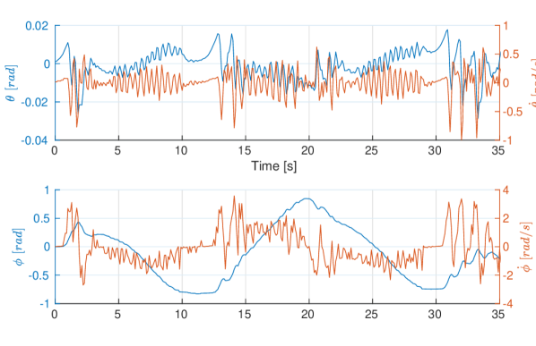
Figure 3: Measured states of the TWIPR while keeping its upright vertical position by employing (12).

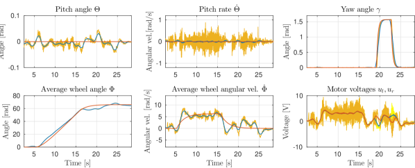
Figure 4: Reference tracking experiment using local controller with a sample time of $35$[ms]. Raw measurements are plotted in yellow, filtered post-processed values in blue, and reference in red. The local controller guarantees stability and reference tracking, despite the noisy measurements.

3.1 Controller Design

Due to limited available input voltages, we choose a linear quadratic regulator (LQR) design, which allows us to balance between performance and control effort, see Aström and Murray (2010). The feedback control law uses the estimated state from Section 2.2, is based on (4), and has the form, $\forall k\in\mathbb{N}_{0}$,

$${\bm{u}}_{d}(k)=-K\bar{\bar{\bm{x}}}(k),$$ (12)

where $K\in\mathbb{R}^{2\times 6}$ is the control gain matrix obtained by minimizing the cost function

$$J=\sum_{k=0}^{\infty}{\bm{x}}_{d}^{\prime}(k)Q{\bm{x}}_{d}(k)+{\bm{u}}_{d}^{\prime}(k)R{\bm{u}}_{d}(k),$$ (13)

with $Q\in\mathbb{R}^{6\times 6}$ and $R\in\mathbb{R}^{2\times 2}$ given. The control gain $K$ is obtained by solving the Algebraic Riccati Equation associated to (13), see (Magni and Scattolini, 2014, p. 171). This controller is responsible for keeping the TWIPR in its upright pose despite disturbances.

3.2 Benchmarking Experiment

In order to facilitate the comparison of different control strategies, benchmarking experiments are defined. The robot body is lifted manually, and measurements (6)–(11) are started. As soon as the measured pitch angle reaches a neighborhood of $0$, say at discrete-time step $\bar{k}\in\mathbb{N}$ corresponding to time $\bar{t}\in\mathbb{R}$, the loop is closed and (12) is applied for all $k\geq\bar{k}$. Results from one trial are presented in Figure 3. The local controller assures that all states remain close to zero.

In order to test a more dynamic and challenging scenario, we also implement the tracking control law

$${\bm{u}}(k)=-K(\bar{\bar{\bm{x}}}(k)-{\bm{x}}_{\text{ref}}(k)),$$ (14)

where ${\bm{x}}_{\text{ref}}(k)$ is a given reference state trajectory. We use the same gain $K$ as for the stabilitation problem, although we should note that it is no longer an optimal feedback gain for the reference tracking task (Anderson et al., 1972, pg. 247). In order to obtain smooth and approximately realizable reference trajectories ${\bm{x}}_{\text{ref}}(k)$, we choose low-pass filtered step changes for $\dot{\Phi}_{\text{ref}}(k)$ and $\gamma_{\text{ref}}(k)$, as illustrated in Figure 4, and determine ${\Phi}_{\text{ref}}(k)$ and $\dot{\gamma}_{\text{ref}}(k)$ by integration and differentiation, respectively. Finally, $\theta_{\text{ref}}(k)$ and $\dot{\theta}_{\text{ref}}(k)$ are chosen constantly zero. Note that a non-zero pitch angle trajectory is required if the robot accelerates and decelerates. However, for the slowly varying velocity reference signals considered in this contribution, zero is a close approximation of that trajectory.

Results from an exemplary run of the experiment are depicted in Figure 4.

The sampling time of $35[\mathrm{ms}]$ could seem large. However, it is required by the employed platform, which does not exhibit state-of-the-art performance. Moreover, future work will study groups of TWIPRs communicating over the channel with orthogonal channel access methods, e.g. TDMA (Time Division Multiple Access), for which this large sampling time is required.

4 Wireless Controller

4.1 Networked Control System Architecture

A NCS is mainly composed of three parts, as illustrated in Figure 1: (i) the plant, in this case the TWIPR, equipped with sensors and actuators. It typically has limited computational power, which is often not enough for hosting the controller on-board; (ii) the communication network, in this case a wireless interface employing the W-LAN protocol; (iii) the controller, in this case executed on a computer with higher computational power.

Data transmission uses W-LAN according to IEEE 802.11g (WiFi) with a transfer rate of 54 Mbit/s in infrastructure mode. Both robot and controller are directly connected to the wireless access point, the controller via the Ethernet adapter Intel I219-LM, the Robot via the wireless dongle Edimax EW-7811Un. The WiFi operates indoor in the 2.4 GHz ISM band, which is shared between multiple wireless technologies such as other WiFi standards and Bluetooth, and employs UDP as a transport protocol. A realistic interfered office environment is used, where several neighboring WiFi networks are coexisting. In this environment, we observed random packet losses due to ”short-time” link failures, which could not be compensated on the communication layer. Zoppi et al. (2019) contains an exhaustive statistical analysis of communication delays for this experimental setup.

At this point, two considerations are derived: (i) experimentally, no packets sent by the robot are lost; this means that the random phenomenon of packet loss occurs only to packets sent by the controller (this asymmetry can be seen in Fig. 1); (ii) all transmitted packets eventually reaching the robot with delays above a given threshold are considered as lost.

Figure 5: Timeline of one control cycle of the NCS. All involved delays and times are analyzed in Zoppi et al. (2019).

4.2 Timing Scheme

Figure 5 shows a timeline of the k-th control cycle. The following times and delays between these steps will be of major relevance in the upcoming sections:

• $t_{m}^{k}$: the robot reads from the sensors. In this moment, the control cycle starts;

• $t_{rh}^{k}$: the controller receives the transmitted packet;

• $t_{rr}^{k}$: the robot receives the control input;

• $d_{c3}^{k}$: time between data reception and actuation;

• $t_{a}^{k}$: instant when the robot applies the desired input to the motors; $t_{a}^{k}-t_{m}^{k}$ is the actuation delay.

From a control perspective, besides dropped packets from controller to robot, also actuation delay must be taken into account, i.e. the control input applied at $t_{a}^{k}$ is computed based on data measured at $t_{m}^{k}$. This actuation delay is time-variant, since, in general, $t_{a}^{k_{1}}-t_{m}^{k_{1}}\not=t_{a}^{k_{2}}-t_{m}^{k_{2}}$, $k_{1},k_{2}\in\mathbb{N}_{0}$.

4.3 Wireless Controller Design

Control packets reach the robot before an arbitrary timeout $\tau_{o}\in\mathbb{R}$ if

$$t_{rr}^{k}-t_{m}^{k}<\tau_{o}<T_{s}.$$ (15)

In the following, if (15) does not hold, the packet is acknowledged as lost. Define a boolean variable that indicates packet loss:

$$\forall k\in\mathbb{N}_{0},\ \epsilon(k)=\begin{cases}1&\text{if }t_{rr}^{k}-t_{m}^{k}\geq\tau_{o}\\ 0&\text{ otherwise}\end{cases}.$$ (16)

So, packets are lost either because never delivered (trivial) or because they would arrive too late at the receiver. To avoid non-deterministic uncertainties resulting from the time-variance of the actuation delay, we deliberately dilate $d_{c3}^{k}$ (by putting a waiting time before the processed signal is applied to the motors) such that

$$\forall k\in\mathbb{N}_{0},\ d_{c3}^{k}=T_{s}-(t_{rr}^{k}-t_{m}^{k}).$$ (17)

In any $k\in\mathbb{N}_{0}$ where (15) holds, by (17), $d_{c3}^{k}>0$. This strategy leads to a larger but constant actuation delay.

We compensate this delay by model-based prediction. Define the following inputs, $\forall k\in\mathbb{N}_{0}$:

$${{\bm{u}}}_{id}(k):=-K{\bm{x}}(t_{a}^{k}),\qquad \hat{{\bm{u}}}(k):=-K\hat{{\bm{x}}}(t_{a}^{k}),$$

where ${{\bm{u}}}_{id}(k)$ is the ideal control input based on states at time of actuation and $\hat{{\bm{u}}}(k)$ is a control input, computed based on a state $\hat{{\bm{x}}}(t_{a}^{k})$ that is predicted from the last available measurement at $t_{m}^{k}$, i.e. $\bar{\bar{\bm{x}}}(k)$. The state is predicted by integrating the nonlinear dynamics (2):

$$\hat{{\bm{x}}}(t_{a}^{k})=\bar{\bar{\bm{x}}}({k})+\int\limits_{t_{m}^{k}}^{t_{m}^{k}+T_{s}}f({\bm{x}}(t),{\bm{u}}(t_{m}^{k}))\mathrm{dt}.$$ (18)

In case (15) does not hold, we use model-based prediction to compensate packet loss. The controller does not know a-priori whether a packet will be lost. Therefore, it calculates and sends a list of $M+1$ control inputs, which are computed based on model-based state predictions of the next $M+1$ steps, where $M$ is chosen larger than the expected maximum number of packet losses. Formally, $\forall k\in\mathbb{N}_{0}$, the controller computes and sends the control input matrix

$$\hat{U}(k):=\left[\hat{{\bm{u}}}(k),{\hat{{\bm{u}}}}(k+1),\dots,{\hat{{\bm{u}}}}(k+M)\right]\in\mathbb{R}^{2\times M+1},$$ (19)

where, $\forall k\in\mathbb{N}_{0},\ \forall i\in\{1,\dots,M\}$,

$${\hat{{\bm{u}}}}(k+i)=-K{\hat{{\bm{x}}}}(t_{a}^{k+i}),$$

with, $\forall k\in\mathbb{N}_{0},\ \forall i\in\{0,\dots,M-1\}$,

$${\hat{{\bm{x}}}}(t_{a}^{k+i+1})={\hat{{\bm{x}}}}(t_{a}^{k+i})+\int\limits_{t_{m}^{k+i}}^{t_{m}^{k+i}+T_{s}}f({\bm{x}}(t),\hat{\bm{u}}({k+i}))\mathrm{dt}.$$ (20)

If the computation time at the remote controller is such that (15) is in general violated, predictions (18) and (20) can be computed using the linearized discrete-time system (5), which is computationally faster but less accurate. The control matrix sent to the robot would, then, be

$${\hat{U}}_{l}(k)=\left[{\hat{{\bm{u}}}}_{l}(k),{\hat{{\bm{u}}}}_{l}(k+1),\dots,{\hat{{\bm{u}}}}_{l}(k+M)\right]\in\mathbb{R}^{2\times M+1},$$

where, $\forall k\in\mathbb{N}_{0},\ \forall i\in\{0,\dots,M\},$

$$\hat{{{\bm{u}}}}_{l}(k+i)=-K{\hat{{\bm{x}}}}_{l}(k+i),$$ (21)

with

$${\hat{{\bm{x}}}}_{l}(k+i)=A_{d}{\hat{{\bm{x}}}}_{l}(k+i-1)+B_{d}\bm{f}_{\mathrm{bl}}\left({\hat{{\bm{u}}}}_{l}(k+i-1)\right)$$ (22)

and ${\hat{{\bm{x}}}}_{l}(k-1)=\bar{\bar{\bm{x}}}({k})$, ${\hat{{\bm{u}}}}_{l}(k-1)={\bm{u}}_{d}({k})$. Then, the most recent control matrix is

$$U^{*}(k):=\begin{cases}{\hat{U}}_{l}(k)&\text{ if }\epsilon(k)=0\\ U^{*}(k-1)&\text{ otherwise}\end{cases},$$ (23)

and the TWIPR applies the control input

$$\forall k\in\mathbb{N}_{0},\;{\bm{u}}(k)=\left[U^{*}(k)\right]_{\omega(k)},$$ (24)

with

$$\omega(k):=1+\min_{\begin{subarray}{c}l\in\left\{0,\dots,M\right\}:\\ \epsilon(k-l)=0\end{subarray}}l$$ (25)

being the number of sampling periods that have passed since the last control matrix was received.

The described Networked Control System is implemented with predictions based on the linearized model (5).

4.4 Experimental Evaluation of the Networked Controller

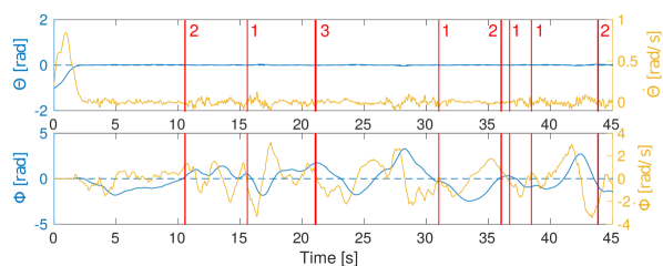
Figure 6: Each red vertical line represents an occurrence of packet loss (the number indicates the amount of sequential packet loss). Although at $t=21[s]$ three control signal packets are lost, the robot does not lose stability.

First, we analyze stability of the proposed NCS and robustness with respect to packet losses. Results are given in Figure 6. Just as the local controller, the networked controller assures that the states remain stable but with clearly larger deviations from zero, at least for the wheel angle.

The proposed networked control strategy is found to exhibit robustness against up to 3 sequential packet losses, i.e. the controller can maintain stability for at least $140[\mathrm{ms}]$ without measurement updates.

The reference tracking experiment described in Section 3.2 is repeated with the proposed networked controller. Result of one trial are given in Figures 7 and 8. Despite two consecutive double packet loss at $t\approx 3.5[\mathrm{s}]$, measurement noise, and actuation delay of $35[\mathrm{ms}]$, the robot does not lose stability.

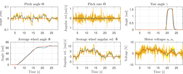
Figure 7: Reference tracking experiment using the NCS with a sampling time of $35$[ms]. Raw measurements are plotted in yellow, filtered post-processed values in blue, and references in red. The networked control strategy exhibits tracks the given references while guaranteeing stability, despite the presence of network delays, packet loss, and measurement noise.

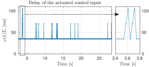
Figure 8: Actuation delay, i.e. $\omega(k)T_{s}$, of every control input.

5 Performance Comparison

We compare the performance of the local and the networked controller for the reference tracking experiment. The local controller has a negligible delay, whereas the networked controller has an actuation delay of $35[\mathrm{ms}]$ (up to $105[\mathrm{ms}]$ in case of packet loss). Performance degradation due to these delays is evaluated by three root mean squared error (RMSE) indices defined by

$$\mathrm{RMSE}_{\Phi}=\sqrt{\frac{1}{k_{\mathrm{end}}-k_{0}}\sum_{k=k_{0}}^{k_{{\mathrm{end}}}}(\bar{\bar{\Phi}}(k)-\Phi_{ref}(k))^{2}},$$

$$\mathrm{RMSE}_{\Theta}=\sqrt{\frac{1}{k_{{\mathrm{end}}}-k_{0}}\sum_{k=k_{0}}^{k_{{\mathrm{end}}}}(\bar{\bar{\Theta}}(k))^{2}},$$

$$\mathrm{RMSE}_{\gamma}=\sqrt{\frac{1}{k_{{\mathrm{end}}}-k_{0}}\sum_{k=k_{0}}^{k_{{\mathrm{end}}}}(\bar{\bar{\gamma}}(k)-\gamma_{ref}(k))^{2}},$$

where $k_{0},k_{end}\in\mathbb{N}$. These RMSE indices are averaged over a set of ten trials. The results are given in Table 2. While differences in $\Phi$- and $\gamma$-movement errors are marginal, RMSE_Θ is almost twice as large for the networked controller than for the local controller, although still small in magnitude.

	Local	NCS
$RMSE_{\Phi}$	2.4141 [rad]	2.4512 [rad]
$RMSE_{\Theta}$	0.0116 [rad]	0.0192 [rad]
$RMSE_{\gamma}$	0.0849 [rad]	0.0888 [rad]

Table 2: RMSE for the states $\Phi$, $\Theta$ and $\gamma$; values for both the local controller and the NCS.

6 Conclusion

In this work, common networked control strategies have been implemented for stabilizing a TWIPR, built with an inexpensive and highly reproducible platform (LEGO Mindstorm EV3). The networked controller is able to stabilize the TWIPR over a wireless channel despite time-varying delays and packet loss. Benchmark experiments have been defined, so that local and remote controllers could be compared.

Future work will consider both practical and theoretical advancements: on one hand, custom hardware is being developed. On the other hand, aiming at improving performance shown in Section 5, both a state observer and an optimal control strategy for reference tracking (computationally more expensive than the solution here adopted) will be employed.

References

- Ananyevskiy and Fradkov (2017) Ananyevskiy, M.S. and Fradkov, A.L. (2017). Control over internet of oscillations for group of pendulums. In Dynamics and Control of Advanced Structures and Machines, 205–213. Springer.
- Anderson et al. (1972) Anderson, B., Moore, J., and Molinari, B. (1972). Linear optimal control. IEEE Transactions on Systems, Man, and Cybernetics, (4), 559–559.
- Aström and Murray (2010) Aström, K.J. and Murray, R.M. (2010). Feedback systems: an introduction for scientists and engineers. Princeton university press.
- Bemporad et al. (2010) Bemporad, A., Heemels, M., and Johansson, M. (2010). Networked control systems, volume 406. Springer.
- Gallenmüller et al. (2018) Gallenmüller, S., Günther, S., Leclaire, M., Zoppi, S., Molinari, F., Schöffauer, R., Kellerer, W., and Carle, G. (2018). Benchmarking networked control systems. In 2018 IEEE Workshop on Benchmarking Cyber-Physical Networks and Systems (CPSBench), 7–12. IEEE.
- Hespanha et al. (2007) Hespanha, J.P., Naghshtabrizi, P., and Xu, Y. (2007). A survey of recent results in networked control systems. Proceedings of the IEEE, 95(1), 138–162.
- Ishii (2008) Ishii, H. (2008). H control with limited communication and message losses. Systems & Control Letters, 57(4), 322–331.
- Kim et al. (2005) Kim, Y., Kim, S.H., and Kwak, Y.K. (2005). Dynamic analysis of a nonholonomic two-wheeled inverted pendulum robot. Journal of Intelligent and Robotic Systems, 44(1), 25–46.
- Magni and Scattolini (2014) Magni, L. and Scattolini, R. (2014). Advanced and multivariable control. Pitagoga edirice Bologna.
- Mori et al. (2014) Mori, T., Kawamura, Y., Zanma, T., and Liu, K. (2014). Compensation of networked control systems with time-delay. In 2014 IEEE 13th International Workshop on Advanced Motion Control (AMC), 752–757. IEEE.
- Nilsson et al. (1998) Nilsson, J., Bernhardsson, B., and Wittenmark, B. (1998). Stochastic analysis and control of real-time systems with random time delays. Automatica, 34(1), 57–64.
- Nordin et al. (1997) Nordin, M., Galic’, J., and Gutman, P.O. (1997). New models for backlash and gear play. International journal of adaptive control and signal processing, 11(1), 49–63.
- Pathak et al. (2005) Pathak, K., Franch, J., and Agrawal, S.K. (2005). Velocity and position control of a wheeled inverted pendulum by partial feedback linearization. IEEE Transactions on robotics, 21(3), 505–513.
- Tin Leung et al. (2011) Tin Leung, K., Whidborne, J.F., Purdy, D., and Dunoyer, A. (2011). A review of ground vehicle dynamic state estimations utilising GPS/INS. Vehicle System Dynamics, 49(1-2), 29–58.
- Walsh et al. (2002) Walsh, G.C., Ye, H., and Bushnell, L.G. (2002). Stability analysis of networked control systems. IEEE transactions on control systems technology, 10(3), 438–446.
- Yu et al. (2008) Yu, J., Wang, L., Yu, M., Jia, Y., and Chen, J. (2008). Stabilizability of networked control systems via packet-loss dependent output feedback controllers. In 2008 American Control Conference, 3620–3625. IEEE.
- Zhang et al. (2016) Zhang, X.M., Han, Q.L., and Yu, X. (2016). Survey on recent advances in networked control systems. IEEE Transactions on Industrial Informatics, 12(5), 1740–1752.
- Zoppi et al. (2019) Zoppi, S., Ayan, O., Molinari, F., Music, Z., Gallenmüller, S., Carle, G., and Kellerer, W. (2019). Reproducible benchmarking platform for networked control systems. In Submitted to IEEE International Conference on Cyber-Physical Systems.