Mean-square approximations of Lévy noise driven SDEs with super-linearly growing diffusion and jump coefficients

Abstract.

This paper first establishes a fundamental mean-square convergence theorem for general one-step numerical approximations of Lévy noise driven stochastic differential equations with non-globally Lipschitz coefficients. Then two novel explicit schemes are designed and their convergence rates are exactly identified via the fundamental theorem. Different from existing works, we do not impose a globally Lipschitz condition on the jump coefficient but formulate appropriate assumptions to allow for its super-linear growth. However, we require that the Lévy measure is finite. New arguments are developed to handle essential difficulties in the convergence analysis, caused by the super-linear growth of the jump coefficient and the fact that higher moment bounds of the Poisson increments $\int_{t}^{t+h}\int_{Z}\,\bar{N}(\mbox{d}s,\mbox{d}z),t\geq 0,h>0$ contribute to magnitude not more than $O(h)$. Numerical results are finally reported to confirm the theoretical findings.

Ziheng Chen, Siqing Gan and Xiaojie Wang^∗

School of Mathematics and Statistics, Central South University

Changsha 410083, Hunan, China

1. Introduction

As a class of important mathematical models, stochastic differential equations (SDEs) driven by Gaussian noise have been widely used in finance, biology, fluid mechanics, chemistry and many other scientific fields. Nevertheless, in the real life one often encounters problems influenced by event-driven uncertainties, which can be captured by jump component. For instance, the stock price movements might suffer from sudden and significant impacts caused by unpredictable important events such as market crashes, announcements made by central banks, changes in credit ratings, etc. In order to model the event-driven phenomena, it is necessary and significant to introduce jump-diffusion SDEs, a typical example of non-Gaussian noise (consult, e.g., [38] for more explanation). Since the analytic solutions of nonlinear SDEs with jumps are rarely available, numerical solutions become a powerful tool to understand the behavior of the underlying problems. Therefore this paper concerns the design and mean-square convergence analysis of discrete-time approximations for jump-diffusion SDEs.

Let $d,m\in\mathbb{N}$, $T>0$ and let $(\Omega,\mathcal{F},\mathbb{P})$ be a complete probability space with a filtration $\{\mathcal{F}_{t}\}_{0\leq{t}\leq{T}}$ satisfying the usual conditions. Let $\{W(t)\}_{0\leq{t}\leq{T}}$ be an $m$-dimensional $\{\mathcal{F}_{t}\}_{0\leq{t}\leq{T}}$-adapted Wiener process. Let $(Z,\mathcal{Z},\nu)$ be a measure space with $Z\subseteq\mathbb{R}^{d}\setminus\{0\}$ and let $N(\mbox{d}t,\mbox{d}z)$ be an $\{\mathcal{F}_{t}\}_{0\leq{t}\leq{T}}$-adapted Poisson random measure defined on $([0,T]\times Z,\mathfrak{B}([0,T]\times Z))$ with $\nu\neq 0$ and $\nu(Z)<\infty$. The compensated Poisson random measure is denoted by $\bar{N}(\mbox{d}t,\mbox{d}z):=N(\mbox{d}t,\mbox{d}z)-\nu(\mbox{d}z)\mbox{d}t$. We consider the following jump-diffusion SDEs

$$\mbox{d}X(t)=f(X(t^{-}))\,\mbox{d}t+g(X(t^{-}))\,\mbox{d}W(t)+\int_{Z}\sigma(X(t^{-}),z)\,\bar{N}(\mbox{d}t,\mbox{d}z),\enskip\forall t\in(0,T]$$ (1)

with $X(0)=X_{0}$, where $X(t^{-})=\lim_{s\nearrow t}X(s),\forall t\in(0,T]$ and the drift coefficient $f\colon\mathbb{R}^{d}\to\mathbb{R}^{d}$, the diffusion coefficient $g\colon\mathbb{R}^{d}\to\mathbb{R}^{{d}\times{m}}$ and the jump coefficient $\sigma\colon\mathbb{R}^{d}\times{Z}\to\mathbb{R}^{d}$ are assumed to be deterministic and Borel measurable. Under further assumptions specified later, a unique solution exists in $L^{2}(\Omega,\mathbb{R}^{d})$ for (1) and its numerical approximation is a central topic of this work.

As the jump component vanishes, i.e., $\sigma\equiv 0$, the underlying jump-diffusion SDEs reduce to the usual SDEs without jumps, numerical methods for which have been extensively studied for the past decades (consult monographs [16, 23, 36] and references therein), in the context of both numerical convergence and numerical stability. Under globally Lipschitz conditions, the corresponding numerical analysis is well-understood [23, 36]. However, coefficients of most models in applications do not obey the classical conditions but, e.g., might behave super-linearly. Recently, Hutzenthaler, Jentzen and Kloeden [17] showed that the standard explicit Euler method produces divergent strong and weak numerical approximations in a finite time interval once one of coefficients grows super-linearly. By contrast, as already shown by Higham, Mao and Stuart [12], Mao and Szpruch [31], Andersson and Kruse[1], the backward (implicit) Euler method, computationally much more expensive than the explicit Euler method, can be strongly convergent under certain non-globally Lipschitz conditions. These observations suggest that special care must be taken to construct and analyze convergent numerical schemes in non-globally Lipschitz setting, and this interesting subject has been investigated in a great portion of the literature [1, 3, 4, 6, 8, 15, 16, 17, 18, 19, 20, 22, 25, 26, 27, 30, 31, 32, 33, 37, 40, 41, 42, 43, 44, 45, 47, 49, 50, 51]. In 2012, Hutzenthaler, Jentzen and Kloeden [18] introduced an explicit method, called the tamed Euler method, to numerically solve SDEs with super-linearly growing drift coefficients and globally Lipschitz diffusion coefficients. Since then, various explicit schemes are designed and analyzed for SDEs with (more general) locally Lipschitz coefficients [3, 4, 6, 15, 16, 19, 26, 27, 32, 33, 40, 41, 42, 44, 45, 47, 49, 50, 51]. Readers can, e.g., refer to [16] for a more comprehensive list of references. Particularly, we should mention a closely relevant article [45] by Tretyakov and Zhang, where a fundamental strong convergence theorem was derived in a non-globally Lipschitz setting, giving an extension of a counterpart in the globally Lipschitz setting [35, 36]. Moreover, an explicit balanced Euler method, given by

$$Y_{n+1}=Y_{n}+\frac{f(Y_{n})h+g(Y_{n})\Delta{W_{n}}}{1+|f(Y_{n})|h+|g(Y_{n})\Delta{W_{n}}|},\quad Y_{0}=X_{0}$$

and a fully implicit Euler method are examined and their convergence rates are obtained, with the aid of the fundamental convergence theorem. Another two closely related papers are [49, 50] by Zhang and Ma, introducing a sine Euler method, defined by

$$Y_{n+1}=Y_{n}+\sin(f(Y_{n})h)+\sin(g(Y_{n})\Delta{W_{n}}),\quad Y_{0}=X_{0}.$$

When $\sigma\not\equiv 0$, the underlying jump-diffusion problem, as a typical non-continuous stochastic process, has been increasingly studied in recent years and a lot of progress has been achieved on numerical analysis of explicit and implicit schemes [5, Deng19, 9, 11, 13, 14, 21, 24, 28, 29, 38, 46, 48]. Particularly, some explicit time-stepping schemes are very recently introduced and their convergence rates are analyzed in non-globally Lipschitz setting [6, Deng19, 25, 26, 44]. However, all existing works on convergence of numerical methods for SDEs with jumps, to the best of our knowledge, impose globally Lipschitz conditions on the jump coefficient (consult the very recent publications [6, 25, 26] and references therein). As pointed out in Chapter 1, Section 9, on Page 59 of [38] by Platen and Bruti-Liberati, for certain applications, the Lipschitz condition on the jump coefficient is too restrictive. For instance, for modeling state-dependent intensities, as discussed in Sect. 1.8 therein, it is convenient to use jump coefficients that are not Lipschitz continuous. This indicates that SDEs with non-globally Lipschitz continuous jump coefficients have applications in certain fields and motivates the present numerical analysis in a more general setting, allowing for non-globally Lipschitz continuous jump coefficients.

We first establish a fundamental mean-square convergence theorem for general one-step numerical methods under certain non-globally Lipschitz conditions (see Assumptions 2.1, 2.3). Although the proof of the fundamental theorem follows the basic lines in previous works [35, 36, 45], some extension of their arguments are made due to the presence of the jump term. For example, new techniques are required and new assumptions (see Assumptions 2.3 and 3.1) are formulated, to treat additional terms resulting from a jump version of the Itô formula. As applications of the fundamental theorem, a new version of the tamed Euler method

$$Y_{n+1}=Y_{n}+\frac{f(Y_{n})h}{1+|f(Y_{n})|h}+\frac{g(Y_{n})\Delta{W_{n}}}{1+|g(Y_{n})|h}+\int_{t_{n}}^{t_{n+1}}\int_{Z}\frac{\sigma(Y_{n},z)}{1+|\sigma(Y_{n},z)|h}\,\bar{N}(\mbox{d}s,\mbox{d}z)$$ (2)

and a so-called sine Euler method

$$Y_{n+1}=Y_{n}+\sin(f(Y_{n})h)+\frac{\sin(g(Y_{n})h)}{h}\Delta{W_{n}}+\int_{t_{n}}^{t_{n+1}}\int_{Z}\frac{\sin(\sigma(Y_{n},z)h)}{h}\,\bar{N}(\mbox{d}s,\mbox{d}z)$$ (3)

are carefully constructed and their mean-square convergence rates are accordingly identified (see Theorems 4.5 and 5.2). The most challenging and technical part in the applications of the fundamental theorem lies on proving boundedness of higher order moments of numerical approximations (see Subsections 4.1 and 5.1). Unlike the Wiener increments $W(t+h)-W(t),t\geq 0,h>0$, higher moment bounds of the Poisson increments $\int_{t}^{t+h}\int_{Z}\,\bar{N}(\mbox{d}s,\mbox{d}z),t\geq 0,h>0$ contribute to magnitude not more than $O(h)$. This significant difference, together with the possible super-linear growth of the jump coefficient, makes the approach used in [45] unworkable here since the nice property of Wiener increments $\mathbb{E}[\|W(t+h)-W(t)\|^{l}]=O(h^{\frac{l}{2}}),l\in\mathbb{N}$ was essentially used there (see the treatment of the last term of (3.6) in [45]), where $\|\cdot\|$ denotes the Euclidean vector norm in $\mathbb{R}^{m}$. This forces us to develop new arguments for the present jump setting. In short, we work with continuous-time approximations of (2) and (3) and carry out rather careful and delicate estimates for all involved terms (see Remark 1 and the proof of Lemma 4.3). Equipped with bounded numerical moments, we examine the local truncation errors of the schemes. This together with the fundamental theorem helps us to obtain the mean-square convergence rates arbitrarily close to the classical order $\tfrac{1}{2}$ (see Theorems 4.5 and 5.2). To the best of our knowledge, this is the first result to identify convergence rates of numerical approximations of jump-diffusion SDEs with possibly super-linearly growing jump coefficients. Moreover, when the jump component vanishes, i.e., $\sigma\equiv 0$, an exact order $\tfrac{1}{2}$ can be attained, see Corollaries 1 and 2, which recovers the relevant results in [1, 16, 18, 31, 40, 41, 45].

Now we compare convergence results in this article with corresponding results in existing literature. The contributions [6, 25] derived the strong convergence rates of different tamed Euler methods for a wider class of Lévy SDEs by allowing $\nu(Z)=\infty$, but with the jump coefficients satisfying the globally Lipschitz conditions, see Assumptions B-3 in [6] and A-8 in [25]. In contrast, we reformulate a more relaxed condition on the jump coefficient to allow for its super-linear growth. Here we require $\nu(Z)<\infty$, which is a limitation compared with [6, 25] and only covers SDEs driven by Wiener process and compound Poisson process. Furthermore, in [6, 25] the $\mathcal{L}^{p}$-convergence rates (for any $p\geq 2$) were obtained, but here we can only get mean-square convergence rates. Finally, to achieve bounded moments of the exact solution, we first show bounded $\bar{p}$-th moments for the highest order $\bar{p}$ being a sufficiently large even number and the general $p$-th moments with arbitrary $p\leq\bar{p}$ follow immediately from the Hölder inequality, see Theorem 2.4.

The remainder of this paper is organized as follows. The next section concerns properties of jump-diffusion SDEs. A fundamental mean-square convergence theorem for general one-step approximations is established in Section 3. In Sections 4 and 5, we propose two new explicit schemes and identify their mean-square convergence rates via the obtained fundamental theorem. Finally numerical experiments are performed to illustrate the theoretical results.

2. Lévy noise driven SDEs with non-globally Lipschitz coefficients

We start with some notation. Let $|\cdot|$ and $\left<\cdot,\cdot\right>$ be the Euclidean norm and the inner product in $\mathbb{R}^{d}$. By $A^{T}$ we denote the transpose of a vector or matrix $A$. If $A$ is a matrix, we let $|A|=\sqrt{\operatorname{trace}(A^{T}A)}$ be its trace norm. If $B$ is a set, its complement and indicator function are denoted by $B^{c}$ and $\mathds{1}_{B}$, respectively. We denote by $L^{r}_{\mathcal{F}_{0}}(\Omega,\mathbb{R}^{d}),r\in\mathbb{N}$ the family of $\mathbb{R}^{d}$-valued $\mathcal{F}_{0}$-measurable random variables $\xi$ with $\mathbb{E}[|\xi|^{r}]<\infty$. For simplicity, the letter $K$ denotes a generic positive constant that is independent of time stepsize and varies for each appearance.

An $\{\mathcal{F}_{t}\}_{0\leq{t}\leq{T}}$-adapted $\mathbb{R}^{d}$-valued stochastic process $\{X(t)\}_{0\leq{t}\leq{T}}$ is called a solution of (1) if it is almost surely right continuous with left limits and satisfies

$$\begin{split}X(t)=X_{0}&+\int_{0}^{t}f(X(s^{-}))\,\mbox{d}s+\int_{0}^{t}g(X(s^{-}))\,\mbox{d}W(s)\\ &+\int_{0}^{t}\int_{Z}\sigma(X(s^{-}),z)\,\bar{N}(\mbox{d}s,\mbox{d}z),~{}~{}\mathbb{P}\text{-a.s.},~{}~{}\forall t\in[0,T].\end{split}$$ (4)

Let us make the following assumption.

Assumption 2.1.

Let $X_{0}\in L^{2}_{\mathcal{F}_{0}}(\Omega,\mathbb{R}^{d})$ and let the mappings $f\colon\mathbb{R}^{d}\to\mathbb{R}^{d}$, $g\colon\mathbb{R}^{d}\to\mathbb{R}^{{d}\times{m}}$, $\sigma(\cdot,z)\colon\mathbb{R}^{d}\to\mathbb{R}^{d},~{}\forall z\in{}Z$ be continuous and satisfy the monotone condition, i.e., there exists $K>0$ such that for all $x,y\in\mathbb{R}^{d}$,

$$2\langle x-y,f(x)-f(y)\rangle+|g(x)-g(y)|^{2}+\int_{Z}|\sigma(x,z)-\sigma(y,z)|^{2}\,\nu(\mbox{d}z)\leq K|x-y|^{2}.$$ (5)

Also let the coefficients satisfy the coercivity condition, i.e., there exists $K>0$ such that

$$2\langle x,f(x)\rangle+|g(x)|^{2}+\int_{Z}|\sigma(x,z)|^{2}\,\nu(\mbox{d}z)\leq K(1+|x|^{2}),\quad\forall x\in\mathbb{R}^{d}.$$ (6)

Let us give the existence of the unique solution to (1), see [10, Theorem 1].

Theorem 2.2.

Let Assumption 2.1 be satisfied. Then (1) admits a unique solution $\{X(t)\}_{0\leq{t}\leq{T}}$ given by (4) and almost all its trajectories are right-continuous with left limits on $[0,T]$.

To discuss the higher order moments of $\{X(t)\}_{0\leq{t}\leq{T}}$, we make the following assumption.

Assumption 2.3.

Let $\varepsilon$ be an arbitrary positive number and let $\bar{p}\geq 2$ be a sufficiently large even number. Assume that $X_{0}\in L^{\bar{p}}_{\mathcal{F}_{0}}(\Omega,\mathbb{R}^{d})$ and that there exists $K>0$ such that

$$\begin{split}\bar{p}|x|^{\bar{p}-2}&\langle x,f(x)\rangle+\tfrac{\bar{p}(\bar{p}-1)}{2}|x|^{\bar{p}-2}|g(x)|^{2}\\ &+\big{(}1+(\bar{p}-2)\varepsilon\big{)}\int_{Z}|\sigma(x,z)|^{\bar{p}}\,\nu(\mbox{d}z)\leq K(1+|x|^{\bar{p}}),\quad\forall x\in\mathbb{R}^{d}.\end{split}$$ (7)

Note that the assumption (7) with $\bar{p}=2$ reduces to (6). We also point out that $\bar{p}$ is the upper order of the bounded moments of the exact solution (see Theorem 2.4) and the parameter $\varepsilon$ comes from proving bounded moments of the exact solution up to order $\bar{p}$ (see (14) and (15) below). With the above setting, we arrive at the following result.

Theorem 2.4.

Suppose Assumptions 2.1, 2.3 hold and let $\{X(t)\}_{0\leq{t}\leq{T}}$ be defined by (4). Let $\bar{p}\geq 2$ coming from (7) be a sufficiently large even number. Then there exists $K>0$ such that

$$\mathbb{E}\big{[}|X(t)|^{\bar{p}}\big{]}\leq K\big{(}1+\mathbb{E}\big{[}|X_{0}|^{\bar{p}}\big{]}\big{)},\quad\forall t\in[0,T].$$ (8)

Before presenting its proof, we provide two elementary facts as follows.

Lemma 2.5.

Let $\rho\in\mathbb{N}$ and $\varepsilon>0$, it holds that

$$|x+y|^{2\rho}-|x|^{2\rho}-2\rho\langle x,y\rangle|x|^{2\rho-2}\leq K|x|^{2\rho}+\big{(}1+(2\rho-2)\varepsilon\big{)}|y|^{2\rho},\quad\forall x,y\in\mathbb{R}^{d}.$$ (9)

Proof.

It follows from the binomial formula that

$$\begin{split}|x+y|^{2\rho}=&\big{(}|x|^{2}+2\left<x,y\right>+|y|^{2}\big{)}^{\rho}=\sum\limits_{i=0}^{\rho}\mbox{C}_{\rho}^{i}|y|^{2i}\big{(}2\left<x,y\right>+|x|^{2}\big{)}^{\rho-i}\\ =&|y|^{2\rho}+\sum\limits_{j=0}^{\rho}\mbox{C}_{\rho}^{j}\big{(}2\left<x,y\right>\big{)}^{j}|x|^{2(\rho-j)}+\sum\limits_{i=1}^{\rho-1}\mbox{C}_{\rho}^{i}|y|^{2i}\big{(}2\left<x,y\right>+|x|^{2}\big{)}^{\rho-i}\\ =&|y|^{2\rho}+|x|^{2\rho}+2\rho\left<x,y\right>|x|^{2\rho-2}+\sum\limits_{j=2}^{\rho}\mbox{C}_{\rho}^{j}\big{(}2\left<x,y\right>\big{)}^{j}|x|^{2(\rho-j)}\\ &+\sum\limits_{i=1}^{\rho-1}\mbox{C}_{\rho}^{i}|y|^{2i}\big{(}2\left<x,y\right>+|x|^{2}\big{)}^{\rho-i}.\end{split}$$ (10)

Employing the Schwarz inequality and the weighted Young inequality guarantees

$$\mbox{C}_{\rho}^{j}\big{(}2\left<x,y\right>\big{)}^{j}|x|^{2(\rho-j)}\leq 2^{j}\mbox{C}_{\rho}^{j}|x|^{2\rho-j}|y|^{j}\leq K_{1}(j)|x|^{2\rho}+\varepsilon|y|^{2\rho},\enskip j=2,\ldots,\rho,$$ (11)

where

$$K_{1}(j)=\tfrac{2\rho-j}{2\rho}\left(2^{j}\mbox{C}_{\rho}^{j}\right)^{\frac{2\rho}{2\rho-j}}\left(\tfrac{2\rho\varepsilon}{j}\right)^{\frac{j}{j-2\rho}},\enskip j=2,\ldots,\rho.$$

Applying the techniques used in (11) and the inequality

$$\big{(}\sum\limits_{i=1}^{n}|a_{i}|\big{)}^{p}\leq n^{p}\sum\limits_{i=1}^{n}|a_{i}|^{p},\quad\forall p>0,a_{i}\in\mathbb{R},i=1,2,\ldots,n,n\in\mathbb{N},$$ (12)

one gets

$$\begin{split}\mbox{C}_{\rho}^{i}|y|^{2i}\big{(}2\left<x,y\right>+|x|^{2}\big{)}^{\rho-i}\leq&2^{2\rho-2i}\mbox{C}_{\rho}^{i}|x|^{\rho-i}|y|^{\rho+i}+2^{\rho-i}\mbox{C}_{\rho}^{i}|x|^{2\rho-2i}|y|^{2i}\\ \leq&\big{(}K_{2}(i)+K_{3}(i)\big{)}|x|^{2\rho}+\varepsilon|y|^{2\rho},\end{split}$$ (13)

where

$$K_{2}(i)=\frac{\rho-i}{2\rho}\big{(}2^{2\rho-2i}\mbox{C}_{\rho}^{i}\big{)}^{\frac{2\rho}{\rho-i}}\big{(}\frac{\rho\varepsilon}{\rho+i}\big{)}^{\frac{\rho+i}{i-\rho}},~{}~{}K_{3}(i)=\frac{\rho-i}{\rho}\big{(}2^{\rho-i}\mbox{C}_{\rho}^{i}\big{)}^{\frac{\rho}{\rho-i}}\big{(}\frac{\rho\varepsilon}{2i}\big{)}^{\frac{i}{i-\rho}}$$

for all $i=1,\ldots,\rho-1$. Then (9) follows by inserting (11) and (13) into (10). ∎

The next lemma is the Itô formula [39, Theorem 33], frequently used later.

Lemma 2.6.

Let $\{X(t)\}_{t\geq 0}$ be a $\mathbb{R}^{d}$-valued stochastic process characterized by (1) and let $V\colon\mathbb{R}^{d}\to\mathbb{R}$ be a continuously twice differentiable function. Then $V(X(t))$ is given by

$$\begin{split}\mbox{d}V(X(t))=&[V_{x}(X(t^{-}))f(X(t^{-}))+\tfrac{1}{2}\operatorname{trace}(g^{T}(X(t^{-}))V_{xx}(X(t^{-})g(X(t^{-})))]\mbox{d}t\\ &+\int_{Z}V(X(t^{-})+\sigma(X(t^{-}),z))-V(X(t^{-}))\bar{N}(\mbox{d}t,\mbox{d}z)\\ &+V_{x}(X(t^{-}))g(X(t^{-}))\,\mbox{d}W(t)+\int_{Z}V(X(t^{-})+\sigma(X(t^{-}),z))\\ &-V(X(t^{-}))-V_{x}(X(t^{-}))\sigma(X(t^{-}),z)\nu(\mbox{d}z)\mbox{d}t,\quad\mathbb{P}\text{-a.s.},\quad\forall t\geq 0.\end{split}$$

At the moment, we are ready to prove Theorem 2.4.

Proof of Theorem 2.4..

For every integer $k\geq 1$, define the stopping times $\tau_{k}=\inf\{t\in[0,T]:|X(t)|>k\},k\in\mathbb{N}$. Clearly $\tau_{k}\uparrow{T}$ as $k\rightarrow\infty,\mathbb{P}\text{-a.s.}$ and $|X(t)|\leq{k}$ for all $0\leq{t}\leq\tau_{k}$. By Lemma 2.6 we can derive that for all $t\in[0,T]$,

$$\begin{split}|X(t)|^{\bar{p}}=&|X_{0}|^{\bar{p}}+{\bar{p}}\int_{0}^{t}|X(s^{-})|^{{\bar{p}}-2}\langle X(s^{-}),f(X(s^{-}))\rangle\,\mbox{d}s\\ &+\frac{{\bar{p}}}{2}\int_{0}^{t}|X(s^{-})|^{{\bar{p}}-2}|g(X(s^{-}))|^{2}\,\mbox{d}s\\ &+\frac{{\bar{p}}({\bar{p}}-2)}{2}\int_{0}^{t}|X(s^{-})|^{{\bar{p}}-4}|X(s^{-})^{T}g(X(s^{-}))|^{2}\,\mbox{d}s\\ &+{\bar{p}}\int_{0}^{t}|X(s^{-})|^{{\bar{p}}-2}\langle X(s^{-}),g(X(s^{-}))\,\mbox{d}W(s)\rangle\\ &+\int_{0}^{t}\int_{Z}|X(s^{-})+\sigma(X(s^{-}),z)|^{\bar{p}}-|X(s^{-})|^{\bar{p}}\,N(\mbox{d}s,\mbox{d}z)\\ &-{\bar{p}}\int_{0}^{t}\int_{Z}|X(s^{-})|^{{\bar{p}}-2}\langle X(s^{-}),\sigma(X(s^{-}),z)\rangle\,\nu(\mbox{d}z)\mbox{d}s,~{}~{}\mathbb{P}\text{-a.s.}.\end{split}$$

This together with Lemma 2.5 results in

$$\begin{split}|X(t)|^{\bar{p}}\leq&|X_{0}|^{\bar{p}}+{\bar{p}}\!\int_{0}^{t}|X(s^{-})|^{{\bar{p}}-2}\langle X(s^{-}),f(X(s^{-}))\rangle\,\mbox{d}s\\ &+\frac{{\bar{p}}({\bar{p}}-1)}{2}\!\int_{0}^{t}|X(s^{-})|^{{\bar{p}}-2}|g(X(s^{-}))|^{2}\,\mbox{d}s\\ &+{\bar{p}}\int_{0}^{t}|X(s^{-})|^{{\bar{p}}-2}\langle X(s^{-}),g(X(s^{-}))\,\mbox{d}W(s)\rangle\\ &+\int_{0}^{t}\int_{Z}|X(s^{-})+\sigma(X(s^{-}),z)|^{\bar{p}}-|X(s^{-})|^{\bar{p}}\,\bar{N}(\mbox{d}s,\mbox{d}z)\\ &+\big{(}1+({\bar{p}}-2)\varepsilon\big{)}\int_{0}^{t}\int_{Z}|\sigma(X(s^{-}),z)|^{\bar{p}}\,\nu(\mbox{d}z)\mbox{d}s\\ &+K\nu(Z)\int_{0}^{t}|X(s^{-})|^{\bar{p}}\,\mbox{d}s,~{}~{}\mathbb{P}\text{-a.s.}.\end{split}$$ (14)

Thanks to (7), $\nu(Z)<\infty$ and the martingale property, we deduce

$$\begin{split}\mathbb{E}\big{[}|X(t\wedge\tau_{k})|^{\bar{p}}\big{]}\leq&K+\mathbb{E}\big{[}|X_{0}|^{\bar{p}}\big{]}+K\int_{0}^{t}\mathbb{E}\big{[}|X(s^{-}\wedge\tau_{k})|^{\bar{p}}\big{]}\,\mbox{d}s\\ \leq&K+\mathbb{E}\big{[}|X_{0}|^{\bar{p}}\big{]}+K\int_{0}^{t}\sup\limits_{0\leq r\leq s}\mathbb{E}\big{[}|X(r\wedge\tau_{k})|^{\bar{p}}\big{]}\,\mbox{d}s,\end{split}$$ (15)

where the properties of the right-continuous with left limits functions [2, Section 2.9] were used in the last step. This immediately gives

$$\sup\limits_{0\leq r\leq t}\mathbb{E}\big{[}|X(r\wedge\tau_{k})|^{\bar{p}}\big{]}\leq K+\mathbb{E}\big{[}|X_{0}|^{\bar{p}}\big{]}+K\int_{0}^{t}\sup\limits_{0\leq r\leq s}\mathbb{E}\big{[}|X(r\wedge\tau_{k})|^{\bar{p}}\big{]}\,\mbox{d}s.$$ (16)

By the Gronwall inequality, one gets

$$\sup\limits_{0\leq r\leq t}\mathbb{E}\big{[}|X(r\wedge\tau_{k})|^{\bar{p}}\big{]}\leq\big{(}K+\mathbb{E}\big{[}|X_{0}|^{\bar{p}}\big{]}\big{)}e^{KT},\quad\forall t\in[0,T].$$

Letting $t=T$, $k\rightarrow\infty$ and applying Fatou’s lemma finish the proof. ∎

Before ending this section, we would like to point out that the condition $\nu(Z)<\infty$ can not be relaxed following our approach. However, one can consult [6, 25], treating SDEs with globally Lipschitz jump coefficients, where the authors used a different approach for the convergence analysis and $\nu(Z)=\infty$ was allowed.

3. A fundamental mean-square convergence theorem

This section aims to establish a fundamental mean-square convergence theorem for general one-step approximation. Given a uniform mesh on $[0,T]$ with $h=\tfrac{T}{N},N\in\mathbb{N}$ being the stepsize, we denote by $X_{t,x}(t+h)$ the solution of (1) at $t+h$ with initial value $X_{t,x}(t)=x$. For $x\in\mathbb{R}^{d}$, $t\in[0,T]$, $h>0$, $0<t+h\leq T$, the general one-step approximation $Y_{t,x}(t+h)$ for $X_{t,x}(t+h)$, depends on $t,x,h,W(t+h)-W(t),\int_{t}^{t+h}\int_{Z}\,\bar{N}(\mbox{d}s,\mbox{d}z)$ and is given by

$$Y_{t,x}(t+h)=x+\Psi\Big{(}t,x,h,W(t+h)-W(t),\int_{t}^{t+h}\int_{Z}\,\bar{N}(\mbox{d}s,\mbox{d}z)\Big{)},$$

where $\Psi$ is a function from $[0,T]\times R^{d}\times(0,T]\times\mathbb{R}^{m}\times\mathbb{R}^{d}$ to $\mathbb{R}^{d}$. By $Y_{t,x}(t+h)$ we denote an approximation of the solution at $t+h$ with initial value $Y_{t,x}(t)=x$. Then one can use $Y_{n+1}=Y_{t_{n},Y_{n}}(t_{n+1})$ to recurrently construct numerical approximations $\{Y_{n}\}_{0\leq{n}\leq{N}}$ on the uniform mesh grid $\{t_{n}=nh,n=0,1,\ldots,N\}$, given by

$$Y_{n+1}=Y_{n}+\Psi\Big{(}t_{n},Y_{n},h,W(t_{n}+h)-W(t_{n}),\int_{t_{n}}^{t_{n}+h}\int_{Z}\,\bar{N}(\mbox{d}s,\mbox{d}z)\Big{)}$$ (17)

for all $n=0,1,\ldots,N-1$ with $Y_{0}=X_{0}$. Alternatively, one can write

$$Y_{n+1}=Y_{t_{n},Y_{n}}(t_{n+1})=Y_{t_{0},Y_{0}}(t_{n+1}),\quad n=0,1,\ldots,N-1.$$

To proceed, we need the following assumption.

Assumption 3.1.

Assume the drift coefficient $f$ of (1) behaves polynomially in the sense that there exist $K,q\geq 0$ such that

$$|f(x)-f(y)|^{2}\leq K(1+|x|^{q}+|y|^{q})|x-y|^{2},\quad\forall x,y\in\mathbb{R}^{d}.$$ (18)

The inequality (18) implies the polynomial growth bound

$$|f(x)|^{2}\leq K(1+|x|^{2+q}),\quad\forall x\in\mathbb{R}^{d}.$$ (19)

This together with (7) further shows that

$$|x|^{\bar{p}-2}|g(x)|^{2}\leq K(1+|x|^{\bar{p}+\frac{q}{2}}),\quad\forall x\in\mathbb{R}^{d},$$ (20)

$$\int_{Z}|\sigma(x,z)|^{\bar{p}}\,\nu(\mbox{d}z)\leq K(1+|x|^{\bar{p}+\frac{q}{2}}),\quad\forall x\in\mathbb{R}^{d}.$$ (21)

Moreover, by virtue of (5) and (18), it is easy to derive

$$|g(x)-g(y)|^{2}\leq K(1+|x|^{\frac{q}{2}}+|y|^{\frac{q}{2}})|x-y|^{2},\quad\forall x,y\in\mathbb{R}^{d},$$ (22)

$$\int_{Z}|\sigma(x,z)-\sigma(y,z)|^{2}\,\nu(\mbox{d}z)\leq K(1+|x|^{\frac{q}{2}}+|y|^{\frac{q}{2}})|x-y|^{2},\quad\forall x,y\in\mathbb{R}^{d}.$$ (23)

Here and below we always assume $h\in(0,h_{0}]$ for some $h_{0}\in(0,1)$.

Lemma 3.2.

Suppose Assumptions 2.1, 2.3, 3.1 hold. Let $\bar{p}$ and $q$ come from (7) and (18), respectively, satisfying $q\leq\bar{p}$. For the representation

$$X_{t,x}(t+h)-X_{t,y}(t+h)=x-y+\Phi_{t,x,y}(t+h),\quad\forall x,y\in\mathbb{R}^{d},$$ (24)

there exists $K>0$ depending on $h_{0}\in(0,1)$ but independent of $h$ such that for all $0<h\leq h_{0},t+h\leq T$,

$$\mathbb{E}\big{[}|X_{t,x}(t+h)-X_{t,y}(t+h)|^{2}\big{]}\leq(1+Kh)|x-y|^{2},\quad \forall x,y\in\mathbb{R}^{d},$$ (25)

$$\mathbb{E}\big{[}|\Phi_{t,x,y}(t+h)|^{2}\big{]}\leq Kh(1+|x|^{q}+|y|^{q})^{\frac{1}{2}}|x-y|^{2},\quad \forall x,y\in\mathbb{R}^{d}.$$ (26)

Proof.

By Lemma 2.6, we infer that for all $0\leq\theta\leq{h}$,

$$\begin{split}&\big{|}X_{t,x}(t+\theta)-X_{t,y}(t+\theta)\big{|}^{2}\\ =&|x-y|^{2}+\int_{t}^{t+\theta}|g(X_{t,x}(s^{-}))-g(X_{t,y}(s^{-}))|^{2}\,\mbox{d}s\\ \end{split}$$

$$\begin{split}&+2\int_{t}^{t+\theta}\langle X_{t,x}(s^{-})-X_{t,y}(s^{-}),f(X_{t,x}(s^{-}))-f(X_{t,y}(s^{-}))\rangle\,\mbox{d}s\\ &-2\int_{t}^{t+\theta}\int_{Z}\langle X_{t,x}(s^{-})-X_{t,y}(s^{-}),\sigma(X_{t,x}(s^{-}),z)-\sigma(X_{t,y}(s^{-}),z)\rangle\,\nu(\mbox{d}z)\mbox{d}s\\ &+2\int_{t}^{t+\theta}\langle X_{t,x}(s^{-})-X_{t,y}(s^{-}),(g(X_{t,x}(s^{-}))-g(X_{t,y}(s^{-})))\,\mbox{d}W(s)\rangle\\ &+\int_{t}^{t+\theta}\int_{Z}|X_{t,x}(s^{-})-X_{t,y}(s^{-})+\sigma(X_{t,x}(s^{-}),z)-\sigma(X_{t,y}(s^{-}),z)|^{2}\\ &-|X_{t,x}(s^{-})-X_{t,y}(s^{-})|^{2}\,N(\mbox{d}s,\mbox{d}z),~{}~{}\mathbb{P}\text{-a.s.}.\end{split}$$

Taking expectations and applying the martingale property imply

$$\begin{split}&\mathbb{E}\big{[}|X_{t,x}(t+\theta)-X_{t,y}(t+\theta)|^{2}\big{]}\\ =&|x-y|^{2}+\int_{t}^{t+\theta}\mathbb{E}\big{[}|g(X_{t,x}(s^{-}))-g(X_{t,y}(s^{-}))|^{2}\big{]}\,\mbox{d}s\\ &+2\int_{t}^{t+\theta}\mathbb{E}\big{[}\langle X_{t,x}(s^{-})-X_{t,y}(s^{-}),f(X_{t,x}(s^{-}))-f(X_{t,y}(s^{-}))\rangle\big{]}\,\mbox{d}s\\ &+\int_{t}^{t+\theta}\mathbb{E}\Big{[}\int_{Z}|\sigma(X_{t,x}(s^{-}),z)-\sigma(X_{t,y}(s^{-}),z)|^{2}\,\nu(\mbox{d}z)\Big{]}\mbox{d}s.\end{split}$$

By the techniques used in (15)–(16), we derive from (5) that

$$\begin{split}&\sup\limits_{t\leq r\leq t+\theta}\mathbb{E}\big{[}|X_{t,x}(r)-X_{t,y}(r)|^{2}\big{]}\\ \leq&|x-y|^{2}+K\int_{t}^{t+\theta}\sup\limits_{t\leq r\leq s}\mathbb{E}\big{[}|X_{t,x}(r)-X_{t,y}(r)|^{2}\big{]}\,\mbox{d}s.\end{split}$$

The Gronwall inequality and the assumption $h\in(0,h_{0}]$ yield

$$\sup\limits_{t\leq r\leq t+\theta}\mathbb{E}\big{[}|X_{t,x}(r)-X_{t,y}(r)|^{2}\big{]}\leq\mbox{e}^{Kh}|x-y|^{2}\leq(1+\bar{K}h)|x-y|^{2}$$ (27)

due to $e^{Kh}\leq 1+\bar{K}h$, where $\bar{K}$ is independent of $h$ but dependent on $h_{0}$. Then (25) is validated by letting $\theta=h$ in (27). For (26), using Lemma 2.6 shows

$$\begin{split}|\Phi_{t,x,y}(t&+\theta)|^{2}=\int_{t}^{t+\theta}|g(X_{t,x}(s^{-}))-g(X_{t,y}(s^{-}))|^{2}\,\mbox{d}s\\ &+2\int_{t}^{t+\theta}\langle\Phi_{t,x,y}(s^{-}),f(X_{t,x}(s^{-}))-f(X_{t,y}(s^{-}))\rangle\,\mbox{d}s\\ &-2\int_{t}^{t+\theta}\int_{Z}\langle\Phi_{t,x,y}(s^{-}),\sigma(X_{t,x}(s^{-}),z)-\sigma(X_{t,y}(s^{-}),z)\rangle\,\nu(\mbox{d}z)\mbox{d}s\\ &+2\int_{t}^{t+\theta}\langle\Phi_{t,x,y}(s^{-}),\left(g(X_{t,x}(s^{-}))-g(X_{t,y}(s^{-}))\right)\mbox{d}W(s)\rangle\\ &+\int_{t}^{t+\theta}\int_{Z}|\Phi_{t,x,y}(s^{-})+\sigma(X_{t,x}(s^{-}),z)-\sigma(X_{t,y}(s^{-}),z)|^{2}\\ &-|\Phi_{t,x,y}(s^{-})|^{2}\,N(\mbox{d}s,\mbox{d}z),~{}\mathbb{P}\text{-a.s.}.\end{split}$$

Taking expectations and using (24) lead to

$$\begin{split}\mathbb{E}\big{[}|\Phi_{t,x,y}(t&+\theta)|^{2}\big{]}=\int_{t}^{t+\theta}\mathbb{E}\big{[}|g(X_{t,x}(s^{-}))-g(X_{t,y}(s^{-}))|^{2}\big{]}\,\mbox{d}s\\ &+2\int_{t}^{t+\theta}\mathbb{E}\big{[}\langle X_{t,x}(s^{-})-X_{t,y}(s^{-}),f(X_{t,x}(s^{-}))-f(X_{t,y}(s^{-}))\rangle\big{]}\,\mbox{d}s\\ &+\int_{t}^{t+\theta}\mathbb{E}\Big{[}\int_{Z}|\sigma(X_{t,x}(s^{-}),z)-\sigma(X_{t,y}(s^{-}),z)|^{2}\,\nu(\mbox{d}z)\Big{]}\mbox{d}s\\ &-2\int_{t}^{t+\theta}\mathbb{E}\big{[}\langle x-y,f(X_{t,x}(s^{-}))-f(X_{t,y}(s^{-}))\rangle\big{]}\,\mbox{d}s.\end{split}$$

With the aid of (5) and the Schwarz inequality, one sees that

$$\begin{split}\mathbb{E}\big{[}|\Phi_{t,x,y}(t+\theta)|^{2}\big{]}\leq&K\int_{t}^{t+\theta}\mathbb{E}\big{[}|X_{t,x}(s^{-})-X_{t,y}(s^{-})|^{2}\big{]}\,\mbox{d}s\\ &+2|x-y|\int_{t}^{t+\theta}\mathbb{E}\big{[}|f(X_{t,x}(s^{-}))-f(X_{t,y}(s^{-}))|\big{]}\,\mbox{d}s.\end{split}$$ (28)

It follows from (8) with $q\leq\bar{p}$, (18), (25) and the Hölder inequality that

$$\begin{split}&\int_{t}^{t+\theta}\mathbb{E}\big{[}|f(X_{t,x}(s^{-}))-f(X_{t,y}(s^{-}))|\big{]}\,\mbox{d}r\\ \leq&\int_{t}^{t+\theta}\mathbb{E}\big{[}\big{(}1+|X_{t,x}(s^{-})|^{q}+|X_{t,y}(s^{-})|^{q}\big{)}^{\frac{1}{2}}\big{|}X_{t,x}(s^{-})-X_{t,y}(s^{-})\big{|}\big{]}\,\mbox{d}r\\ \leq&\int_{t}^{t+\theta}\big{(}1+\mathbb{E}\big{[}|X_{t,x}(s^{-})|^{q}\big{]}+\mathbb{E}\big{[}|X_{t,y}(s^{-})|^{q}\big{]}\big{)}^{\frac{1}{2}}\\ &~{}~{}~{}\hskip 10.00002pt\times\big{(}\mathbb{E}\big{[}|X_{t,x}(s^{-})-X_{t,y}(s^{-})|^{2}\big{]}\big{)}^{\frac{1}{2}}\,\mbox{d}r\\ \leq&K\theta\big{(}1+|x|^{q}+|y|^{q}\big{)}^{\frac{1}{2}}|x-y|.\end{split}$$ (29)

Plugging (24), (29) into (28) and using (12), the properties of the right-continuous with left limits functions [2, Section 2.9] give

$$\begin{split}\mathbb{E}\big{[}|\Phi_{t,x,y}(t+&\theta)|^{2}\big{]}\leq K\theta\big{(}1+|x|^{q}+|y|^{q}\big{)}^{\frac{1}{2}}|x-y|^{2}+K\int_{t}^{t+\theta}\mathbb{E}\big{[}|\Phi_{t,x,y}(r^{-})|^{2}\big{]}\,\mbox{d}r\\ \leq&K\theta\big{(}1+|x|^{q}+|y|^{q}\big{)}^{\frac{1}{2}}|x-y|^{2}+K\int_{t}^{t+\theta}\sup_{t\leq s\leq r}\mathbb{E}\big{[}|\Phi_{t,x,y}(s)|^{2}\big{]}\,\mbox{d}r,\end{split}$$

which immediately shows

$$\sup_{t\leq s\leq t+\theta}\mathbb{E}\big{[}|\Phi_{t,x,y}(s)|^{2}\big{]}\leq K\theta\big{(}1+|x|^{q}+|y|^{q}\big{)}^{\frac{1}{2}}|x-y|^{2}+K\int_{t}^{t+\theta}\sup_{t\leq s\leq r}\mathbb{E}\big{[}|\Phi_{t,x,y}(s)|^{2}\big{]}\,\mbox{d}r.$$

By the Gronwall inequality, we get

$$\sup_{t\leq s\leq t+\theta}\mathbb{E}\big{[}|\Phi_{t,x,y}(s)|^{2}\big{]}\leq K\theta\big{(}1+|x|^{q}+|y|^{q}\big{)}^{\frac{1}{2}}|x-y|^{2},\quad\forall\theta\in[0,h],$$

and consequently

$$\mathbb{E}\big{[}|\Phi_{t,x,y}(t+\theta)|^{2}\big{]}\leq K\theta\big{(}1+|x|^{q}+|y|^{q}\big{)}^{\frac{1}{2}}|x-y|^{2},\quad\forall\theta\in[0,h],$$

which gives the desired result (26) by taking $\theta=h$. ∎

Equipped with the above lemma, we are ready to build up the fundamental mean-square convergence theorem for numerical approximations of (1).

Theorem 3.3.

Let Assumptions 2.1, 2.3, 3.1 be satisfied and let $\bar{p}$ and $q$ come from (7) and (18), respectively, satisfying $q\leq\bar{p}$. Suppose that the one-step approximation $Y_{t,x}(t+h)$ defined by (17) has the following local orders of accuracy, i.e., there exist $h_{0}\in(0,1)$, $K>0$, and $\alpha\geq 1$ such that for any $h\in(0,h_{0}]$, $t+h\leq T,x\in\mathbb{R}^{d}$,

$$\big{|}\mathbb{E}\big{[}X_{t,x}(t+h)-Y_{t,x}(t+h)\big{]}\big{|}\leq K\big{(}1+|x|^{2\alpha}\big{)}^{\frac{1}{2}}h^{p_{1}},$$ (30)

$$\big{(}\mathbb{E}\big{[}|X_{t,x}(t+h)-Y_{t,x}(t+h)|^{2}\big{]}\big{)}^{\frac{1}{2}}\leq K\big{(}1+|x|^{2\alpha}\big{)}^{\frac{1}{2}}h^{p_{2}}$$ (31)

with

$$p_{2}\geq\tfrac{1}{2},\quad p_{1}\geq{p_{2}+\tfrac{1}{2}}.$$ (32)

Moreover, the approximation $\{Y_{n}\}_{0\leq n\leq N}$ produced by (17) has finite $p$-th moments, i.e., for sufficiently large $p\geq 2$ there exist $K>0,\beta>0$ such that for any $h\in(0,h_{0}]$,

$$\sup_{0\leq n\leq N}\mathbb{E}\big{[}|Y_{n}|^{p}\big{]}\leq K\big{(}1+\big{(}\mathbb{E}[|X_{0}|^{\bar{p}}]\big{)}^{\beta}\big{)}.$$ (33)

Then there exists $\gamma>0$ and $K>0$ independent of $h$ such that

$$\sup_{0\leq n\leq N}\left(\mathbb{E}[|X(t_{n})-Y_{n}|^{2}]\right)^{\frac{1}{2}}\leq K\big{(}1+(\mathbb{E}[|X_{0}|^{\bar{p}}])^{\gamma}\big{)}h^{p_{2}-\frac{1}{2}}.$$

Proof.

Since

$$\begin{split}X(t_{n+1})-&Y_{n+1}=X_{t_{0},X_{0}}(t_{n+1})-Y_{t_{0},Y_{0}}(t_{n+1})=X_{t_{n},X(t_{n})}(t_{n+1})-Y_{t_{n},Y_{n}}(t_{n+1})\\ =&\big{(}X_{t_{n},X(t_{n})}(t_{n+1})-X_{t_{n},Y_{n}}(t_{n+1})\big{)}+\big{(}X_{t_{n},Y_{n}}(t_{n+1})-Y_{t_{n},Y_{n}}(t_{n+1})\big{)},\end{split}$$

one can arrive at

$$\begin{split}\mathbb{E}\big{[}&|X(t_{n+1})-Y_{n+1}|^{2}\big{]}=\mathbb{E}\big{[}|X_{t_{n},X(t_{n})}(t_{n+1})-X_{t_{n},Y_{n}}(t_{n+1})|^{2}\big{]}\\ &+2\mathbb{E}\big{[}\langle X_{t_{n},X(t_{n})}(t_{n+1})-X_{t_{n},Y_{n}}(t_{n+1}),X_{t_{n},Y_{n}}(t_{n+1})-Y_{t_{n},Y_{n}}(t_{n+1})\rangle\big{]}\\ &+\mathbb{E}\big{[}|X_{t_{n},Y_{n}}(t_{n+1})-Y_{t_{n},Y_{n}}(t_{n+1})|^{2}\big{]}:=A_{1}+A_{2}+A_{3}.\end{split}$$ (34)

Thanks to the conditional version of (25), we have

$$A_{1}=\mathbb{E}\big{[}\mathbb{E}\big{(}|X_{t_{n},X(t_{n})}(t_{n+1})-X_{t_{n},Y_{n}}(t_{n+1})|^{2}\big{|}\mathcal{F}_{t_{n}}\big{)}\big{]}\leq(1+Kh)\mathbb{E}\big{[}|X(t_{n})-Y_{n}|^{2}\big{]}.$$

Likewise, the conditional version of (31) ensures that

$$A_{3}=\mathbb{E}\big{[}\mathbb{E}\big{(}|X_{t_{n},Y_{n}}(t_{n+1})-Y_{t_{n},Y_{n}}(t_{n+1})|^{2}\big{|}\mathcal{F}_{t_{n}}\big{)}\big{]}\leq Kh^{2p_{2}}\mathbb{E}\big{[}(1+|Y_{n}|^{2\alpha})\big{]}.$$

It remains to estimate $A_{2}$. Using (24) leads to

$$\begin{split}A_{2}=&2\mathbb{E}\big{[}\langle\Phi_{t_{n},X(t_{n}),Y_{n}}(t_{n+1}),X_{t_{n},Y_{n}}(t_{n+1})-Y_{t_{n},Y_{n}}(t_{n+1})\rangle\big{]}\\ &+2\mathbb{E}\big{[}\langle X(t_{n})-Y_{n},X_{t_{n},Y_{n}}(t_{n+1})-Y_{t_{n},Y_{n}}(t_{n+1})\rangle\big{]}:=A_{21}+A_{22}.\end{split}$$ (35)

Before estimating $A_{21}$, we put the conditional versions of (26) and (31) here,

$$\mathbb{E}\big{(}|\Phi_{t_{n},X(t_{n}),Y_{n}}(t_{n}+h)|^{2}\big{|}\mathcal{F}_{t_{n}}\big{)}\leq Kh\big{(}1+|X(t_{n})|^{q}+|Y_{n}|^{q}\big{)}^{\frac{1}{2}}\big{|}X(t_{n})-Y_{n}\big{|}^{2},$$

$$\mathbb{E}\big{(}|X_{t_{n},Y_{n}}(t_{n}+h)-Y_{t_{n},Y_{n}}(t_{n}+h)|^{2}\big{|}\mathcal{F}_{t_{n}}\big{)}\leq K\big{(}1+|Y_{n}|^{2\alpha}\big{)}h^{2p_{2}}.$$

By the Schwarz inequality, the conditional version of the Hölder inequality and the $\mathcal{F}_{t_{n}}$-measurability of $X(t_{n})-Y_{n}$, we get

$$\begin{split}&A_{21}=2\mathbb{E}\big{[}\mathbb{E}\big{(}\big{\langle}\Phi_{t_{n},X(t_{n}),Y_{n}}(t_{n+1}),X_{t_{n},Y_{n}}(t_{n+1})-Y_{t_{n},Y_{n}}(t_{n+1})\big{\rangle}\big{|}\mathcal{F}_{t_{n}}\big{)}\big{]}\\ \leq&2\mathbb{E}\big{[}\big{(}\mathbb{E}(|\Phi_{t_{n},X(t_{n}),Y_{n}}(t_{n+1})|^{2}|\mathcal{F}_{t_{n}})\big{)}^{\frac{1}{2}}\big{(}\mathbb{E}\big{(}|X_{t_{n},Y_{n}}(t_{n+1})-Y_{t_{n},Y_{n}}(t_{n+1})|^{2}\big{|}\mathcal{F}_{t_{n}}\big{)}\big{)}^{\frac{1}{2}}\big{]}\\ \leq&Kh^{p_{2}+\frac{1}{2}}\mathbb{E}\big{[}(1+|X(t_{n})|^{q}+|Y_{n}|^{q})^{\frac{1}{4}}|X(t_{n})-Y_{n}|(1+|Y_{n}|^{2\alpha})^{\frac{1}{2}}\big{]}\\ =&K\mathbb{E}\big{[}h^{\frac{1}{2}}|X(t_{n})-Y_{n}|\times h^{p_{2}}(1+|X(t_{n})|^{q}+|Y_{n}|^{q})^{\frac{1}{4}}(1+|Y_{n}|^{2\alpha})^{\frac{1}{2}}\big{]}\\ \leq&Kh\mathbb{E}\big{[}|X(t_{n})-Y_{n}|^{2}\big{]}+Kh^{2p_{2}}\mathbb{E}\big{[}\big{(}1+|Y_{n}|^{2\alpha}\big{)}\big{(}1+|X(t_{n})|^{q}+|Y_{n}|^{q}\big{)}^{\frac{1}{2}}\big{]},\end{split}$$

where the weighted Young inequality $ab\leq\varepsilon a^{2}+\frac{b^{2}}{4\varepsilon}$ for all $a,b\in\mathbb{R}$ with $\varepsilon=\frac{1}{2}>0$ was used in the last step. The $\mathcal{F}_{t_{n}}$-measurability of $X(t_{n})-Y_{n}$, $p_{1}\geq p_{2}+\frac{1}{2}$, the Hölder inequality and the conditional version of (30) imply

$$\begin{split}A_{22}=&2\mathbb{E}\big{[}\big{\langle}X(t_{n})-Y_{n},\mathbb{E}\big{(}X_{t_{n},Y_{n}}(t_{n+1})-Y_{t_{n},Y_{n}}(t_{n+1})\big{|}\mathcal{F}_{t_{n}}\big{)}\big{\rangle}\big{]}\\ \leq&2\big{(}\mathbb{E}\big{[}|X(t_{n})-Y_{n}|^{2}\big{]}\big{)}^{\frac{1}{2}}\big{(}\mathbb{E}\big{[}\big{|}\mathbb{E}((X_{t_{n},Y_{n}}(t_{n+1})-Y_{t_{n},Y_{n}}(t_{n+1}))|\mathcal{F}_{t_{n}})\big{|}^{2}\big{]}\big{)}^{\frac{1}{2}}\\ \leq&Kh^{p_{1}}\big{(}\mathbb{E}\big{[}|X(t_{n})-Y_{n}|^{2}\big{]}\big{)}^{\frac{1}{2}}\mathbb{E}\big{[}1+|Y_{n}|^{2\alpha}\big{]}^{\frac{1}{2}}.\\ \leq&Kh^{p_{2}+\frac{1}{2}}\big{(}\mathbb{E}\big{[}|X(t_{n})-Y_{n}|^{2}\big{]}\big{)}^{\frac{1}{2}}\mathbb{E}\big{[}1+|Y_{n}|^{2\alpha}\big{]}^{\frac{1}{2}}\\ \leq&Kh\mathbb{E}\big{[}|X(t_{n})-Y_{n}|^{2}\big{]}+Kh^{2p_{2}}\mathbb{E}\big{[}1+|Y_{n}|^{2\alpha}\big{]}.\end{split}$$

Inserting $A_{21}$ and $A_{22}$ into (35), we get

$$A_{2}\leq Kh\mathbb{E}\big{[}|X(t_{n})-Y_{n}|^{2}\big{]}+Kh^{2p_{2}}\mathbb{E}\big{[}(1+|Y_{n}|^{2\alpha})\big{(}1+|X(t_{n})|^{q}+|Y_{n}|^{q}\big{)}^{\frac{1}{2}}\big{]}.$$

Substituting $A_{1},A_{2},A_{3}$ into (34) and using (8) with $q\leq\bar{p}$, (33) tell that

$$\begin{split}\mathbb{E}\big{[}|X(t_{n+1})-Y_{n+1}|^{2}\big{]}\leq&(1+Kh)\mathbb{E}\big{[}|X(t_{n})-Y_{n}|^{2}\big{]}+Kh^{2p_{2}}\big{(}1+\big{(}\mathbb{E}[|X_{0}|^{\bar{p}}]\big{)}^{\beta+\frac{q}{2\bar{p}}}\big{)},\end{split}$$

which immediately gives

$$\begin{split}&\mathbb{E}\big{[}|X(t_{n})-Y_{n}|^{2}\big{]}-\mathbb{E}\big{[}|X(t_{n-1})-Y_{n-1}|^{2}\big{]}\\ \leq&Kh\mathbb{E}\big{[}|X(t_{n-1})-Y_{n-1}|^{2}\big{]}+Kh^{2p_{2}}\big{(}1+\big{(}\mathbb{E}[|X_{0}|^{\bar{p}}]\big{)}^{\beta+\frac{q}{2\bar{p}}}\big{)}.\end{split}$$

By summation, $X(t_{0})=X_{0}=Y_{0}$ and $nh\leq T$, we have

$$\begin{split}\mathbb{E}\big{[}|X(t_{n})-Y_{n}|^{2}\big{]}\leq Kh\sum\limits_{i=1}^{n-1}\mathbb{E}\big{[}|X(t_{i})-Y_{i}|^{2}\big{]}+Kh^{2p_{2}-1}\big{(}1+\big{(}\mathbb{E}[|X_{0}|^{\bar{p}}]\big{)}^{\beta+\frac{q}{2\bar{p}}}\big{)}.\end{split}$$

Exploiting the discrete Gronwall inequality (see, e.g., [30, Lemma 3.4]) and using $nh\leq T$ again result in the desired result. ∎

4. Application of the fundamental convergence theorem: convergence rates of the tamed Euler method

As the first application of the fundamental mean-square convergence theorem, we shall construct a new version of the tamed Euler method, also named the tamed Euler method, as follows

$$Y_{n+1}=Y_{n}+\frac{f(Y_{n})h}{1+|f(Y_{n})|h}+\frac{g(Y_{n})\Delta{W_{n}}}{1+|g(Y_{n})|h}+\int_{t_{n}}^{t_{n+1}}\int_{Z}\frac{\sigma(Y_{n},z)}{1+|\sigma(Y_{n},z)|h}\,\bar{N}(\mbox{d}s,\mbox{d}z)$$ (36)

with $Y_{0}=X_{0}$, where $\Delta{W_{n}}:=W(t_{n+1})-W(t_{n}),n=0,1,\ldots,N-1$. The scheme is different from schemes introduced by Tretyakov and Zhang [45] even the jump term vanishes, i.e., $\sigma\equiv 0$. To apply Theorem 3.3, it is crucial to obtain the boundedness of the higher-order moments of $\{Y_{n}\}_{0\leq n\leq N}$ given by (36).

4.1. Bounded $p$-th moments of the tamed Euler method

We will present some lemmas before showing the boundedness of $p$-th moments of $\{Y_{n}\}_{0\leq n\leq N}$. The first one is the Burkholder-Davis-Gundy (BDG) inequality (see [34, Lemma 1]).

Lemma 4.1 (Burkholder-Davis-Gundy inequality).

Suppose $p\geq 1$ and let $\mathcal{P}$ be the progressive $\sigma$-algebra on $[0,\infty)\times\Omega$ and $\mathfrak{B}(Z)$ be the Borel $\sigma$-algebra of $Z$. If $\phi$ is a $\mathcal{P}\otimes\mathfrak{B}(Z)$-measurable function such that $\mathbb{P}$-a.s. $\int_{0}^{T}\int_{Z}|\phi(s,z)|^{2}\,\nu(\mbox{d}z)\mbox{d}s<\infty.$ Then there exists $K>0$ such that for all $p\geq 2$,

$$\begin{split}\mathbb{E}\bigg{[}\sup_{0\leq{t}\leq{T}}\Big{|}\int_{0}^{t}\int_{Z}\phi(s,z)\,\bar{N}(\mbox{d}s,\mbox{d}z)\Big{|}^{p}\bigg{]}\leq&K\mathbb{E}\Big{[}\int_{0}^{T}\int_{Z}|\phi(s,z)|^{2}\nu(\mbox{d}z)\mbox{d}s\Big{]}^{\frac{p}{2}}\\ &+K\mathbb{E}\Big{[}\int_{0}^{T}\int_{Z}|\phi(s,z)|^{p}\nu(\mbox{d}z)\,\mbox{d}s\Big{]}.\end{split}$$ (37)

Moreover, if $1\leq p<2$, then the last term of (37) can be omitted.

Unlike the BDG inequality for the Wiener process, the $p$-th moments ($p\geq 1$) of the Poisson increments $\int_{t}^{t+h}\int_{Z}\bar{N}(\mbox{d}s,\mbox{d}z),t\geq 0,h>0$ contribute to magnitude not more than $O(h)$. This, as already discussed earlier, causes significant difficulties in proving bounded $p$-th moments of the tamed Euler method. Additionally, we need the following elementary inequality.

Lemma 4.2.

Let $1\leq l\in\mathbb{N}$. Then there exists $K:=K(l)>0$ such that

$$\big{|}|x|^{2l}-|y|^{2l}\big{|}\leq K\sum\limits_{i=1}^{2l}|x-y|^{i}|y|^{{2l}-i},\quad\forall x,y\in\mathbb{R}^{d},$$

where, as a conventional notation, we set $y^{0}=1$.

Proof.

We derive from the binomial formula and (12) that for all $x,y\in\mathbb{R}^{d}$,

$$\begin{split}&\big{|}|x|^{2l}-|y|^{2l}\big{|}=\big{|}\langle x-y+y,x-y+y\rangle^{l}-|y|^{2l}\big{|}\\ =&\big{|}\big{(}|x-y|^{2}+2\langle x-y,y\rangle+|y|^{2}\big{)}^{l}-|y|^{2l}\big{|}\\ =&\Big{|}\sum\limits_{i=1}^{l}\mbox{C}_{l}^{i}\big{(}|x-y|^{2}+2\langle x-y,y\rangle\big{)}^{i}|y|^{2(l-i)}\Big{|}\\ \leq&K\sum\limits_{i=1}^{l}\Big{(}|x-y|^{2i}|y|^{2l-2i}+|x-y|^{i}|y|^{2l-i}\Big{)}\\ \leq&K\sum\limits_{i=1}^{2l}|x-y|^{i}|y|^{2l-i},\end{split}$$

which completes the proof. ∎

We will prove that the numerical approximations produced by (36) enjoy bounded high-order moments. At first, we show that the boundedness of high-order moments remains valid within a family of appropriate subevents. Before doing so, we would like to add some comments here.

Remark 1.

It is worthwhile to emphasize that, one can not simply extend the analysis in [45] to the present jump setting, because the property of Wiener increments $\mathbb{E}[\|W(t+h)-W(t)\|^{l}]=O(h^{\frac{l}{2}}),l\in\mathbb{N}$ was essentially used there (see the treatment of the last term of (3.6) in [45]) while, as clarified earlier, the Poisson increments violate such nice property and the jump coefficients might grow super-linearly.

To overcome the above difficulty, we work with continuous-time approximations and do very careful estimates. Let $R>0$ be sufficiently large and define a sequence of decreasing subevents

$$\Omega_{R,n}:=\{\omega\in\Omega:\sup_{0\leq i\leq n}|Y_{i}(\omega)|\leq R\},\quad\forall n=0,1,\ldots,N,\,\,N\in\mathbb{N}.$$

Obviously, $\mathds{1}_{\Omega_{R(h),n}}$ are $\mathcal{F}_{t_{n}}$-measurable for all $n=0,1,\ldots,N$. The next result indicates that moments of $\{Y_{n}\}_{0\leq n\leq N}$ are bounded on the subevents $\Omega_{R,n}$.

Lemma 4.3.

Suppose Assumptions 2.1, 2.3, 3.1 hold. Let $\bar{p}\geq 2$ coming from (7) be a sufficiently large even number and let $\{Y_{n}\}_{0\leq n\leq N}$ be given by (36). Then there exist $R=h^{-H(q)^{-1}}:=R(h)$ with $H(q)=\max\left\{1+q,\tfrac{3}{2}q\right\}$ and $K>0$ independent of $h$ such that

$$\sup_{0\leq n\leq N}\mathbb{E}\big{[}\mathds{1}_{\Omega_{R(h),n}}|Y_{n}|^{\bar{p}}\big{]} \leq K\big{(}1+\mathbb{E}\big{[}|X_{0}|^{\bar{p}}\big{]}\big{)},$$ (38)

$$\sup_{0\leq n\leq N-1}\mathbb{E}\big{[}\mathds{1}_{\Omega_{R(h),n}}|Y_{n+1}|^{\bar{p}}\big{]} \leq K\big{(}1+\mathbb{E}\big{[}|X_{0}|^{\bar{p}}\big{]}\big{)}.$$ (39)

Proof.

We define a continuous-time version $\{\bar{Y}(t)\}_{0\leq{t}\leq{T}}$ of $\{Y_{n}\}_{0\leq{n}\leq{N}}$ by

$$\begin{split}\bar{Y}(t)=&Y_{n}+\int_{t_{n}}^{t}\frac{f(Y_{n})}{1+|f(Y_{n})|h}\,\mbox{d}s+\int_{t_{n}}^{t}\frac{g(Y_{n})}{1+|g(Y_{n})|h}\,\mbox{d}W(s)\\ &+\int_{t_{n}}^{t}\int_{Z}\frac{\sigma(Y_{n},z)}{1+|\sigma(Y_{n},z)|h}\,\bar{N}(\mbox{d}s,\mbox{d}z),~{}~{}\mathbb{P}\text{-a.s.}\end{split}$$ (40)

for all $t\in[t_{n},t_{n+1}],n=0,1,\ldots,N-1$. Applying Lemma 2.6 yields

$$\begin{split}|\bar{Y}(t)|^{\bar{p}}=&|Y_{n}|^{\bar{p}}+{\bar{p}}\int_{t_{n}}^{t}|\bar{Y}(s^{-})|^{{\bar{p}}-2}\Big{\langle}\bar{Y}(s^{-}),\frac{f(Y_{n})}{1+|f(Y_{n})|h}\Big{\rangle}\,\mbox{d}s\\ &+\frac{{\bar{p}}}{2}\int_{t_{n}}^{t}|\bar{Y}(s^{-})|^{{\bar{p}}-2}\Big{|}\frac{g(Y_{n})}{1+|g(Y_{n})|h}\Big{|}^{2}\,\mbox{d}s\\ &+\frac{{\bar{p}}({\bar{p}}-2)}{2}\int_{t_{n}}^{t}|\bar{Y}(s^{-})|^{{\bar{p}}-4}\Big{|}\frac{\bar{Y}(s^{-})^{T}g(Y_{n})}{1+|g(Y_{n})|h}\Big{|}^{2}\,\mbox{d}s\\ &+{\bar{p}}\int_{t_{n}}^{t}|\bar{Y}(s^{-})|^{{\bar{p}}-2}\Big{\langle}\bar{Y}(s^{-}),\frac{g(Y_{n})\,\mbox{d}W(s)}{1+|g(Y_{n})|h}\Big{\rangle}\\ &+\int_{t_{n}}^{t}\int_{Z}\Big{|}\bar{Y}(s^{-})+\frac{\sigma(Y_{n},z)}{1+|\sigma(Y_{n},z)|h}\Big{|}^{{\bar{p}}}-|\bar{Y}(s^{-})|^{{\bar{p}}}\,N(\mbox{d}s,\mbox{d}z)\\ &-{\bar{p}}\int_{t_{n}}^{t}\int_{Z}|\bar{Y}(s^{-})|^{{\bar{p}}-2}\Big{\langle}\bar{Y}(s^{-}),\frac{\sigma(Y_{n},z)}{1+|\sigma(Y_{n},z)|h}\Big{\rangle}\,\nu(\mbox{d}z)\mbox{d}s,\quad\mathbb{P}\text{-a.s.}.\end{split}$$

Then we use the Schwarz inequality and Lemma 2.5 to get

$$\begin{split}|\bar{Y}(t)|^{\bar{p}}\leq&|Y_{n}|^{\bar{p}}+{\bar{p}}\int_{t_{n}}^{t}|\bar{Y}(s^{-})|^{{\bar{p}}-2}\Big{\langle}\bar{Y}(s^{-}),\frac{f(Y_{n})}{1+|f(Y_{n})|h}\Big{\rangle}\,\mbox{d}s\\ &+\frac{\bar{p}(\bar{p}-1)}{2}\int_{t_{n}}^{t}|\bar{Y}(s^{-})|^{\bar{p}-2}\Big{|}\frac{g(Y_{n})}{1+|g(Y_{n})|h}\Big{|}^{2}\,\mbox{d}s\end{split}$$

$$\begin{split}&+\bar{p}\int_{t_{n}}^{t}|\bar{Y}(s^{-})|^{\bar{p}-2}\Big{\langle}\bar{Y}(s^{-}),\frac{g(Y_{n})\,\mbox{d}W(s)}{1+|g(Y_{n})|h}\Big{\rangle}+K\int_{t_{n}}^{t}|\bar{Y}(s^{-})|^{\bar{p}}\,\mbox{d}s\\ &+\int_{t_{n}}^{t}\int_{Z}\Big{|}\bar{Y}(s^{-})+\frac{\sigma(Y_{n},z)}{1+|\sigma(Y_{n},z)|h}\Big{|}^{\bar{p}}-|\bar{Y}(s^{-})|^{\bar{p}}\,\bar{N}(\mbox{d}s,\mbox{d}z)\\ &+\big{(}1+(\bar{p}-2)\varepsilon\big{)}\int_{t_{n}}^{t}\int_{Z}\Big{|}\frac{\sigma(Y_{n},z)}{1+|\sigma(Y_{n},z)|h}\Big{|}^{\bar{p}}\,\nu(\mbox{d}z)\mbox{d}s,\quad\mathbb{P}\text{-a.s.}.\end{split}$$

As a result,

$$\begin{split}&\mathbb{E}\big{[}\mathds{1}_{\Omega_{R,n}}|\bar{Y}(t)|^{\bar{p}}\big{]}\\ \leq&\mathbb{E}\big{[}\mathds{1}_{\Omega_{R,n}}|Y_{n}|^{\bar{p}}\big{]}+\bar{p}\int_{t_{n}}^{t}\mathbb{E}\Big{[}\mathds{1}_{\Omega_{R,n}}|\bar{Y}(s^{-})|^{\bar{p}-2}\Big{\langle}\bar{Y}(s^{-}),\frac{f(Y_{n})}{1+|f(Y_{n})|h}\Big{\rangle}\Big{]}\,\mbox{d}s\\ &+\frac{\bar{p}(\bar{p}-1)}{2}\int_{t_{n}}^{t}\mathbb{E}\big{[}\mathds{1}_{\Omega_{R,n}}|\bar{Y}(s^{-})|^{\bar{p}-2}|g(Y_{n})|^{2}\big{]}\,\mbox{d}s+K\int_{t_{n}}^{t}\mathbb{E}\big{[}\mathds{1}_{\Omega_{R,n}}|\bar{Y}(s^{-})|^{\bar{p}}\big{]}\,\mbox{d}s\\ &+\big{(}1+(\bar{p}-2)\varepsilon\big{)}\int_{t_{n}}^{t}\mathbb{E}\Big{[}\mathds{1}_{\Omega_{R,n}}\int_{Z}|\sigma(Y_{n},z)|^{\bar{p}}\,\nu(\mbox{d}z)\Big{]}\mbox{d}s\\ =&\mathbb{E}\big{[}\mathds{1}_{\Omega_{R,n}}|Y_{n}|^{\bar{p}}\big{]}+\bar{p}\int_{t_{n}}^{t}\mathbb{E}\big{[}\mathds{1}_{\Omega_{R,n}}|Y_{n}|^{\bar{p}-2}\langle Y_{n},f(Y_{n})\rangle\big{]}\,\mbox{d}s\\ &+\frac{\bar{p}(\bar{p}-1)}{2}\int_{t_{n}}^{t}\mathbb{E}\big{[}\mathds{1}_{\Omega_{R,n}}|Y_{n}|^{\bar{p}-2}|g(Y_{n})|^{2}\big{]}\,\mbox{d}s+K\int_{t_{n}}^{t}\mathbb{E}\big{[}\mathds{1}_{\Omega_{R,n}}|\bar{Y}(s^{-})|^{\bar{p}}\big{]}\,\mbox{d}s\\ &+\big{(}1+(\bar{p}-2)\varepsilon\big{)}\int_{t_{n}}^{t}\mathbb{E}\Big{[}\mathds{1}_{\Omega_{R,n}}\int_{Z}|\sigma(Y_{n},z)|^{\bar{p}}\,\nu(\mbox{d}z)\Big{]}\mbox{d}s+I_{1}+I_{2}+I_{3}+I_{4},\end{split}$$

where

$$I_{1}:= \bar{p}\int_{t_{n}}^{t}\mathbb{E}\Big{[}\mathds{1}_{\Omega_{R,n}}\big{|}\bar{Y}(s^{-})\big{|}^{\bar{p}-2}\Big{\langle}\bar{Y}(s^{-})-Y_{n},\frac{f(Y_{n})}{1+|f(Y_{n})|h}\Big{\rangle}\Big{]}\,\mbox{d}s,$$

$$I_{2}:= \bar{p}\int_{t_{n}}^{t}\mathbb{E}\Big{[}\mathds{1}_{\Omega_{R,n}}|\bar{Y}(s^{-})|^{\bar{p}-2}\Big{\langle}Y_{n},\frac{f(Y_{n})}{1+|f(Y_{n})|h}-f(Y_{n})\Big{\rangle}\Big{]}\,\mbox{d}s,$$

$$I_{3}:= \bar{p}\int_{t_{n}}^{t}\mathbb{E}\big{[}\mathds{1}_{\Omega_{R,n}}\big{(}|\bar{Y}(s^{-})|^{\bar{p}-2}-|Y_{n}|^{\bar{p}-2}\big{)}\langle Y_{n},f(Y_{n})\rangle\big{]}\,\mbox{d}s,$$

$$I_{4}:= \frac{\bar{p}(\bar{p}-1)}{2}\int_{t_{n}}^{t}\mathbb{E}\big{[}\mathds{1}_{\Omega_{R,n}}\big{(}|\bar{Y}(s^{-})|^{\bar{p}-2}-|Y_{n}|^{\bar{p}-2}\big{)}|g(Y_{n})|^{2}\big{]}\,\mbox{d}s.$$

Using the coercivity condition (7) yields

$$\begin{split}\mathbb{E}[\mathds{1}_{\Omega_{R,n}}|\bar{Y}(t)|^{\bar{p}}]\leq&(1+Kh)\mathbb{E}[\mathds{1}_{\Omega_{R,n}}|Y_{n}|^{\bar{p}}]+K\int_{t_{n}}^{t}\mathbb{E}[\mathds{1}_{\Omega_{R,n}}|\bar{Y}(s^{-})|^{\bar{p}}]\,\mbox{d}s\\ &+I_{1}+I_{2}+I_{3}+I_{4}.\end{split}$$ (41)

For $I_{1}$, using the Schwarz inequality and (12) helps us to get

$$\begin{split}I_{1}\leq&\bar{p}\int_{t_{n}}^{t}\mathbb{E}\big{[}\mathds{1}_{\Omega_{R,n}}|\bar{Y}(s^{-})|^{\bar{p}-2}|\bar{Y}(s^{-})-Y_{n}||f(Y_{n})|\big{]}\mbox{d}s\\ \leq&K\!\int_{t_{n}}^{t}\!\mathbb{E}\big{[}\mathds{1}_{\Omega_{R,n}}|\bar{Y}(s^{-})-Y_{n}|^{\bar{p}-1}|f(Y_{n})|\big{]}\mbox{d}s\\ &+K\!\int_{t_{n}}^{t}\!\mathbb{E}\big{[}\mathds{1}_{\Omega_{R,n}}|\bar{Y}(s^{-})-Y_{n}||f(Y_{n})||Y_{n}|^{\bar{p}-2}\big{]}\mbox{d}s:=I_{11}+I_{12}.\end{split}$$ (42)

It follows from (40) and (12) that

$$\begin{split}I_{11}\leq&K\int_{t_{n}}^{t}\mathbb{E}\Big{[}\mathds{1}_{\Omega_{R,n}}|f(Y_{n})|\Big{|}\frac{(s-t_{n})f(Y_{n})}{1+|f(Y_{n})|h}\Big{|}^{\bar{p}-1}\Big{]}\,\mbox{d}s\\ &+K\int_{t_{n}}^{t}\mathbb{E}\Big{[}\mathds{1}_{\Omega_{R,n}}|f(Y_{n})|\Big{|}\frac{g(Y_{n})(W(s)-W(t_{n}))}{1+|g(Y_{n})|h}\Big{|}^{\bar{p}-1}\Big{]}\,\mbox{d}s\\ &+K\int_{t_{n}}^{t}\mathbb{E}\Big{[}\mathds{1}_{\Omega_{R,n}}|f(Y_{n})|\Big{|}\int_{t_{n}}^{s}\int_{Z}\frac{\sigma(Y_{n},z)}{1+|\sigma(Y_{n},z)|h}\,\bar{N}(\mbox{d}r,\mbox{d}z)\Big{|}^{\bar{p}-1}\Big{]}\,\mbox{d}s\\ \leq&Kh^{\bar{p}}\mathbb{E}\big{[}\mathds{1}_{\Omega_{R,n}}|f(Y_{n})|^{\bar{p}}\big{]}+Kh^{\frac{\bar{p}+1}{2}}\mathbb{E}\big{[}\mathds{1}_{\Omega_{R,n}}|f(Y_{n})||g(Y_{n})|^{\bar{p}-1}\big{]}\\ &+Kh\mathbb{E}\Big{[}\sup_{t_{n}\leq{s}\leq{t}}\Big{|}\int_{t_{n}}^{s}\int_{Z}\frac{\mathds{1}_{\Omega_{R,n}}\sigma(Y_{n},z)|f(Y_{n})|^{\frac{1}{\bar{p}-1}}}{1+|\sigma(Y_{n},z)|h}\,\bar{N}(\mbox{d}r,\mbox{d}z)\Big{|}^{\bar{p}-1}\Big{]}.\end{split}$$ (43)

We then use Lemma 4.1, (19), (20) and (21) to obtain

$$\begin{split}I_{11}\leq&Kh^{\bar{p}}\mathbb{E}\big{[}\mathds{1}_{\Omega_{R,n}}|f(Y_{n})|^{\bar{p}}\big{]}+Kh^{\frac{\bar{p}+1}{2}}\mathbb{E}\big{[}\mathds{1}_{\Omega_{R,n}}|f(Y_{n})||g(Y_{n})|^{\bar{p}-1}\big{]}\\ &+Kh^{\frac{\bar{p}+1}{2}}\mathbb{E}\Big{[}\mathds{1}_{\Omega_{R,n}}|f(Y_{n})|\Big{(}\int_{Z}|\sigma(Y_{n},z)|^{2}\,\nu(\mbox{d}z)\Big{)}^{\frac{\bar{p}-1}{2}}\Big{]}\\ &+Kh^{2}\mathbb{E}\Big{[}\mathds{1}_{\Omega_{R,n}}|f(Y_{n})|\int_{Z}|\sigma(Y_{n},z)|^{\bar{p}-1}\,\nu(\mbox{d}z)\Big{]}\\ \leq&Kh+Kh^{\bar{p}}\mathbb{E}\big{[}\mathds{1}_{\Omega_{R,n}}|Y_{n}|^{\bar{p}+\frac{\bar{p}q}{2}}\big{]}+Kh^{\frac{\bar{p}+1}{2}}\mathbb{E}\big{[}\mathds{1}_{\Omega_{R,n}}|Y_{n}|^{\bar{p}+\frac{(\bar{p}+1)q}{4}}\big{]}\\ &+Kh^{2}\mathbb{E}\big{[}\mathds{1}_{\Omega_{R,n}}|Y_{n}|^{\bar{p}+q}\big{]}.\end{split}$$ (44)

Repeating the same arguments used in (43) and (44) implies

$$\begin{split}I_{12}\leq&\int_{t_{n}}^{t}\mathbb{E}\Big{[}\mathds{1}_{\Omega_{R,n}}|f(Y_{n})||Y_{n}|^{\bar{p}-2}\Big{|}\frac{(s-t_{n})f(Y_{n})}{1+|f(Y_{n})|h}\Big{|}\Big{]}\,\mbox{d}s\\ &+\int_{t_{n}}^{t}\mathbb{E}\Big{[}\mathds{1}_{\Omega_{R,n}}|f(Y_{n})||Y_{n}|^{\bar{p}-2}\Big{|}\frac{g(Y_{n})(W(s)-W(t_{n}))}{1+|g(Y_{n})|h}\Big{|}\Big{]}\,\mbox{d}s\\ &+\int_{t_{n}}^{t}\mathbb{E}\Big{[}\mathds{1}_{\Omega_{R,n}}|f(Y_{n})||Y_{n}|^{\bar{p}-2}\Big{|}\int_{t_{n}}^{s}\int_{Z}\frac{\sigma(Y_{n},z)}{1+|\sigma(Y_{n},z)|h}\,\bar{N}(\mbox{d}r,\mbox{d}z)\Big{|}\Big{]}\,\mbox{d}s\end{split}$$

and thus

$$\begin{split}I_{12}\leq&h^{2}\mathbb{E}\big{[}\mathds{1}_{\Omega_{R,n}}|f(Y_{n})|^{2}|Y_{n}|^{\bar{p}-2}\big{]}+h^{\frac{3}{2}}\mathbb{E}\big{[}\mathds{1}_{\Omega_{R,n}}|g(Y_{n})||f(Y_{n})||Y_{n}|^{\bar{p}-2}\big{]}\\ &+h\mathbb{E}\Big{[}\sup_{t_{n}\leq{s}\leq{t}}\Big{|}\int_{t_{n}}^{s}\int_{Z}\frac{\mathds{1}_{\Omega_{R,n}}\sigma(Y_{n},z)|f(Y_{n})||Y_{n}|^{\bar{p}-2}}{1+|\sigma(Y_{n},z)|h}\,\bar{N}(\mbox{d}r,\mbox{d}z)\Big{|}\Big{]}\\ \leq&h^{2}\mathbb{E}\big{[}\mathds{1}_{\Omega_{R,n}}|f(Y_{n})|^{2}|Y_{n}|^{\bar{p}-2}\big{]}+h^{\frac{3}{2}}\mathbb{E}\big{[}\mathds{1}_{\Omega_{R,n}}|g(Y_{n})||f(Y_{n})||Y_{n}|^{\bar{p}-2}\big{]}\\ &+Kh^{\frac{3}{2}}\mathbb{E}\Big{[}\mathds{1}_{\Omega_{R,n}}|f(Y_{n})||Y_{n}|^{\bar{p}-2}\Big{(}\int_{Z}|\sigma(Y_{n},z)|\,\nu(\mbox{d}z)\Big{)}^{\frac{1}{2}}\Big{]}\\ \leq&Kh+Kh^{2}\mathbb{E}\big{[}\mathds{1}_{\Omega_{R,n}}|Y_{n}|^{\bar{p}+q}\big{]}+Kh^{\frac{3}{2}}\mathbb{E}\big{[}\mathds{1}_{\Omega_{R,n}}|Y_{n}|^{\bar{p}+\frac{3q}{4}}\big{]}.\end{split}$$

Substituting the above $I_{11}$ and $I_{12}$ into (42) gives

$$\begin{split}I_{1}\leq&Kh+Kh^{\bar{p}}\mathbb{E}\big{[}\mathds{1}_{\Omega_{R,n}}|Y_{n}|^{\bar{p}+\frac{\bar{p}q}{2}}\big{]}+Kh^{\frac{\bar{p}+1}{2}}\mathbb{E}\big{[}\mathds{1}_{\Omega_{R,n}}|Y_{n}|^{\bar{p}+\frac{(\bar{p}+1)q}{4}}\big{]}\\ &+Kh^{2}\mathbb{E}\big{[}\mathds{1}_{\Omega_{R,n}}|Y_{n}|^{\bar{p}+q}\big{]}+Kh^{\frac{3}{2}}\mathbb{E}\big{[}\mathds{1}_{\Omega_{R,n}}|Y_{n}|^{\bar{p}+\frac{3q}{4}}\big{]}.\end{split}$$ (45)

Treating $I_{2}$ by the Schwarz inequality, the Young inequality and (19) leads to

$$\begin{split}I_{2}\leq&\bar{p}\int_{t_{n}}^{t}\mathbb{E}\big{[}\mathds{1}_{\Omega_{R,n}}|\bar{Y}(s^{-})|^{\bar{p}-2}|Y_{n}||f(Y_{n})|^{2}h\big{]}\,\mbox{d}s\\ \leq&(\bar{p}-2)\int_{t_{n}}^{t}\mathbb{E}\big{[}\mathds{1}_{\Omega_{R,n}}|\bar{Y}(s^{-})|^{\bar{p}}\big{]}\,\mbox{d}s+2h^{1+\frac{\bar{p}}{2}}\mathbb{E}\big{[}\mathds{1}_{\Omega_{R,n}}|Y_{n}|^{\frac{\bar{p}}{2}}|f(Y_{n})|^{\bar{p}}\big{]}\\ \leq&(\bar{p}-2)\int_{t_{n}}^{t}\mathbb{E}\big{[}\mathds{1}_{\Omega_{R,n}}|\bar{Y}(s^{-})|^{\bar{p}}\big{]}\,\mbox{d}s+Kh+Kh^{1+\frac{\bar{p}}{2}}\mathbb{E}\big{[}\mathds{1}_{\Omega_{R,n}}|Y_{n}|^{\frac{3+q}{2}\bar{p}}\big{]}.\end{split}$$ (46)

By the Schwarz inequality, Lemma 4.2 and (40), we have

$$\begin{split}&I_{3}\leq\bar{p}\int_{t_{n}}^{t}\mathbb{E}\big{[}\mathds{1}_{\Omega_{R,n}}\big{|}|\bar{Y}(s^{-})|^{\bar{p}-2}-|Y_{n}|^{\bar{p}-2}\big{|}|Y_{n}||f(Y_{n})|\big{]}\,\mbox{d}s\\ \leq&K\sum\limits_{i=1}^{\bar{p}-2}\int_{t_{n}}^{t}\mathbb{E}\big{[}\mathds{1}_{\Omega_{R,n}}|\bar{Y}(s^{-})-Y_{n}|^{i}|Y_{n}|^{\bar{p}-1-i}|f(Y_{n})|\big{]}\,\mbox{d}s\\ \leq&K\sum\limits_{i=1}^{\bar{p}-2}h^{i+1}\mathbb{E}\big{[}\mathds{1}_{\Omega_{R,n}}|f(Y_{n})|^{i+1}|Y_{n}|^{\bar{p}-1-i}\big{]}\\ &+K\sum\limits_{i=1}^{\bar{p}-2}h^{\frac{i}{2}+1}\mathbb{E}\big{[}\mathds{1}_{\Omega_{R,n}}|g(Y_{n})|^{i}|Y_{n}|^{\bar{p}-1-i}|f(Y_{n})|\big{]}\\ &+Kh\sum\limits_{i=1}^{\bar{p}-2}\mathbb{E}\Big{[}\sup_{t_{n}\leq{s}\leq{t}}\Big{|}\int_{t_{n}}^{s}\int_{Z}\frac{\mathds{1}_{\Omega_{R,n}}\sigma(Y_{n},z)(|Y_{n}|^{\bar{p}-1-i}|f(Y_{n})|)^{\frac{1}{i}}}{1+|\sigma(Y_{n},z)|h}\,\bar{N}(\mbox{d}r,\mbox{d}z)\Big{|}^{i}\Big{]}.\end{split}$$

The techniques used in (43)–(44) further tell us that

$$\begin{split}I_{3}\leq&K\sum\limits_{i=1}^{\bar{p}-2}h^{i+1}\mathbb{E}\big{[}\mathds{1}_{\Omega_{R,n}}|f(Y_{n})|^{i+1}|Y_{n}|^{\bar{p}-1-i}\big{]}\\ &+K\sum\limits_{i=1}^{\bar{p}-2}h^{\frac{i}{2}+1}\mathbb{E}\big{[}\mathds{1}_{\Omega_{R,n}}|g(Y_{n})|^{i}|Y_{n}|^{\bar{p}-1-i}|f(Y_{n})|\big{]}\\ &+K\sum\limits_{i=1}^{\bar{p}-2}h^{\frac{i}{2}+1}\mathbb{E}\Big{[}\mathds{1}_{\Omega_{R,n}}|Y_{n}|^{\bar{p}-1-i}|f(Y_{n})|\Big{(}\int_{Z}|\sigma(Y_{n},z)|^{2}\,\nu(\mbox{d}z)\Big{)}^{\frac{i}{2}}\Big{]}\\ &+Kh^{2}\sum\limits_{i=1}^{\bar{p}-2}\mathbb{E}\Big{[}\mathds{1}_{\Omega_{R,n}}|Y_{n}|^{\bar{p}-1-i}|f(Y_{n})|\int_{Z}|\sigma(Y_{n},z)|^{i}\,\nu(\mbox{d}z)\Big{]}\\ \leq&Kh+K\sum\limits_{i=1}^{\bar{p}-2}h^{i+1}\mathbb{E}\big{[}\mathds{1}_{\Omega_{R,n}}|Y_{n}|^{\bar{p}+\frac{i+1}{2}q}\big{]}+K\sum\limits_{i=1}^{\bar{p}-2}h^{\frac{i}{2}+1}\mathbb{E}\big{[}\mathds{1}_{\Omega_{R,n}}|Y_{n}|^{\bar{p}+\frac{i+2}{4}q}\big{]}.\end{split}$$

Similarly,

$$\begin{split}I_{4}\leq&K\sum\limits_{i=1}^{\bar{p}-2}\int_{t_{n}}^{t}\mathbb{E}\big{[}\mathds{1}_{\Omega_{R,n}}|\bar{Y}(s^{-})-Y_{n}|^{i}|g(Y_{n})|^{2}|Y_{n}|^{\bar{p}-2-i}\big{]}\,\mbox{d}s\\ \leq&Kh+K\sum\limits_{i=1}^{\bar{p}-2}h^{i+1}\mathbb{E}\big{[}\mathds{1}_{\Omega_{R,n}}|Y_{n}|^{\bar{p}+\frac{1+i}{2}q}\big{]}+K\sum\limits_{i=1}^{\bar{p}-2}h^{\frac{i}{2}+1}\mathbb{E}\big{[}\mathds{1}_{\Omega_{R,n}}|Y_{n}|^{\bar{p}+\frac{2+i}{4}q}\big{]}.\end{split}$$

Inserting $I_{1}$, $I_{2}$, $I_{3}$ and $I_{4}$ into (41) promises

$$\begin{split}\mathbb{E}\big{[}\mathds{1}_{\Omega_{R,n}}&|\bar{Y}(t)|^{\bar{p}}\big{]}\leq Kh+(1+Kh)\mathbb{E}\big{[}\mathds{1}_{\Omega_{R,n}}|Y_{n}|^{\bar{p}}\big{]}\\ &+K\int_{t_{n}}^{t}\mathbb{E}\big{[}\mathds{1}_{\Omega_{R,n}}|\bar{Y}(s^{-})|^{\bar{p}}\big{]}\,\mbox{d}s+Kh^{1+\frac{\bar{p}}{2}}\mathbb{E}\big{[}\mathds{1}_{\Omega_{R,n}}|Y_{n}|^{\frac{3+q}{2}\bar{p}}\big{]}\\ &+K\sum\limits_{i=1}^{\bar{p}-1}h^{i+1}\mathbb{E}\big{[}\mathds{1}_{\Omega_{R,n}}|Y_{n}|^{\bar{p}+\frac{i+1}{2}q}\big{]}+K\sum\limits_{i=1}^{\bar{p}-1}h^{\frac{i}{2}+1}\mathbb{E}\big{[}\mathds{1}_{\Omega_{R,n}}|Y_{n}|^{\bar{p}+\frac{i+2}{4}q}\big{]}.\end{split}$$

Choosing $R=R(h)=h^{-H(q)^{-1}}$ with $H(q)=\max\left\{1+q,\tfrac{3}{2}q\right\}$, one can easily get $\mathds{1}_{\Omega_{R(h),n}}|Y_{n}|\leq h^{-H(q)^{-1}}$ and for all $i=1,\ldots,\bar{p}-1$,

$$\mathds{1}_{\Omega_{R(h),n}}|Y_{n}|^{1+q}h\leq h^{1-(1+q)H(q)^{-1}}\leq h_{0}^{1-(1+q)H(q)^{-1}},$$

$$\mathds{1}_{\Omega_{R(h),n}}|Y_{n}|^{\frac{1+1/i}{2}q}h\leq h^{1-\frac{1+1/i}{2}qH(q)^{-1}}\leq h_{0}^{1-\frac{1+1/i}{2}qH(q)^{-1}},$$

$$\mathds{1}_{\Omega_{R(h),n}}|Y_{n}|^{\frac{1+2/i}{2}q}h\leq h^{1-\frac{1+2/i}{2}qH(q)^{-1}}\leq h_{0}^{1-\frac{1+2/i}{2}qH(q)^{-1}}.$$

These inequalities immediately show that for all $i=1,\ldots,\bar{p}-1$,

$$\mathds{1}_{\Omega_{R,n}}|Y_{n}|^{\frac{3+q}{2}\bar{p}}h^{\frac{\bar{p}}{2}}=\mathds{1}_{\Omega_{R(h),n}}|Y_{n}|^{\bar{p}}\big{(}\mathds{1}_{\Omega_{R(h),n}}|Y_{n}|^{1+q}h\big{)}^{\frac{\bar{p}}{2}} \leq K\mathds{1}_{\Omega_{R(h),n}}|Y_{n}|^{\bar{p}},$$

$$\mathds{1}_{\Omega_{R,n}}|Y_{n}|^{\bar{p}+\frac{i+1}{2}q}h^{i}=\mathds{1}_{\Omega_{R(h),n}}|Y_{n}|^{\bar{p}}\big{(}\mathds{1}_{\Omega_{R(h),n}}|Y_{n}|^{\frac{1+1/i}{2}q}h\big{)}^{i} \leq K\mathds{1}_{\Omega_{R(h),n}}|Y_{n}|^{\bar{p}},$$

$$\mathds{1}_{\Omega_{R,n}}|Y_{n}|^{\bar{p}+\frac{i+2}{4}q}h^{\frac{i}{2}}=\mathds{1}_{\Omega_{R(h),n}}|Y_{n}|^{\bar{p}}\big{(}\mathds{1}_{\Omega_{R(h),n}}|Y_{n}|^{\frac{1+2/i}{2}q}h\big{)}^{\frac{i}{2}} \leq K\mathds{1}_{\Omega_{R(h),n}}|Y_{n}|^{\bar{p}},$$

where the constants $K$ are independent of stepsize $h$. Thus

$$\mathbb{E}\big{[}\mathds{1}_{\Omega_{R(h),n}}|\bar{Y}(t)|^{\bar{p}}\big{]}\leq Kh+(1+Kh)\mathbb{E}\big{[}\mathds{1}_{\Omega_{R(h),n}}|Y_{n}|^{\bar{p}}\big{]}+K\int_{t_{n}}^{t}\mathbb{E}\big{[}\mathds{1}_{\Omega_{R(h),n}}|\bar{Y}(s^{-})|^{\bar{p}}\big{]}\,\mbox{d}s.$$

Following the techniques used in (15)–(16), we have

$$\begin{split}\sup\limits_{t_{n}\leq r\leq t}\mathbb{E}[\mathds{1}_{\Omega_{R(h),n}}|\bar{Y}(r)|^{\bar{p}}]\leq&Kh+(1+Kh)\mathbb{E}[\mathds{1}_{\Omega_{R(h),n}}|Y_{n}|^{\bar{p}}]\\ &+K\int_{t_{n}}^{t}\sup\limits_{t_{n}\leq r\leq s}\mathbb{E}[\mathds{1}_{\Omega_{R(h),n}}|\bar{Y}(r)|^{\bar{p}}]\,\mbox{d}s.\end{split}$$

The Gronwall inequality shows that for all $t\in[t_{n},t_{n+1}]$,

$$\sup\limits_{t_{n}\leq r\leq t}\mathbb{E}\big{[}\mathds{1}_{\Omega_{R(h),n}}|\bar{Y}(r)|^{\bar{p}}\big{]}\leq Khe^{Kh}+(1+Kh)e^{Kh}\mathbb{E}\big{[}\mathds{1}_{\Omega_{R(h),n}}|Y_{n}|^{\bar{p}}\big{]}.$$

Taking $t=t_{n+1}$ and repeating the treatment used in (27) particularly yield

$$\mathbb{E}\big{[}\mathds{1}_{\Omega_{R(h),n}}|Y_{n+1}|^{\bar{p}}\big{]}\leq Kh+(1+Kh)\mathbb{E}\big{[}\mathds{1}_{\Omega_{R(h),n}}|Y_{n}|^{\bar{p}}\big{]}.$$ (47)

By the decreasing property of $\{\Omega_{R,n}\}_{0\leq n\leq N}$, we get $\mathds{1}_{\Omega_{R(h),n+1}}\leq\mathds{1}_{\Omega_{R(h),n}}$ and

$$\mathbb{E}\big{[}\mathds{1}_{\Omega_{R(h),n+1}}|Y_{n+1}|^{\bar{p}}\big{]}\leq\mathbb{E}\big{[}\mathds{1}_{\Omega_{R(h),n}}|Y_{n+1}|^{\bar{p}}\big{]}\leq Kh+(1+Kh)\mathbb{E}\big{[}\mathds{1}_{\Omega_{R(h),n}}|Y_{n}|^{\bar{p}}\big{]},$$

which obviously shows

$$\mathbb{E}\big{[}\mathds{1}_{\Omega_{R(h),n}}|Y_{n}|^{\bar{p}}\big{]}\leq Knh+\mathbb{E}\big{[}\mathds{1}_{\Omega_{R(h),0}}|Y_{0}|^{\bar{p}}\big{]}+Kh\sum\limits_{i=0}^{n-1}\mathbb{E}\big{[}\mathds{1}_{\Omega_{R(h),i}}|Y_{i}|^{\bar{p}}\big{]}.$$

Applying the discrete Gronwall inequality (see, e.g., [30, Lemma 3.4]) and using $nh\leq T$ guarantee (38), which together with (47) and $0<h\leq h_{0}$ immediately suggests (39). Thus we complete the proof. ∎

Equipped with the previous lemma, one can derive bounded moments of (36).

Lemma 4.4.

Suppose Assumptions 2.1, 2.3, 3.1 hold and let $\{Y_{n}\}_{0\leq n\leq N}$ be given by (36). Let $H(q)=\max\left\{1+q,\tfrac{3}{2}q\right\}$ and let $\bar{p}\geq 2+4H(q)$ be a sufficiently large even number. Then there exist $\beta>0$ and $K>0$ independent of $h$ such that

$$\sup\limits_{0\leq n\leq N}\mathbb{E}\big{[}|Y_{n}|^{p}\big{]}\leq K\big{(}1+\big{(}\mathbb{E}[|X_{0}|^{\bar{p}}]\big{)}^{\beta}\big{)},\quad\forall p\in\big{[}2,\tfrac{\bar{p}-H(q)}{1+\frac{3}{2}H(q)}\big{]}.$$ (48)

Proof.

It follows from (36) that

$$\begin{split}|Y_{n+1}|&\leq|Y_{n}|+\frac{|f(Y_{n})|h}{1+|f(Y_{n})|h}+\frac{|g(Y_{n})\Delta{W_{n}}|}{1+|g(Y_{n})|h}\\ &+\Big{|}\int_{t_{n}}^{t_{n+1}}\int_{Z}\frac{\sigma(Y_{n},z)}{1+|\sigma(Y_{n},z)|h}\,\bar{N}(\mbox{d}s,\mbox{d}z)\Big{|}\\ \leq&|Y_{n}|+1+\frac{|\Delta{W_{n}}|}{h}+\nu(Z)+\int_{t_{n}}^{t_{n+1}}\int_{Z}\frac{1}{h}\,N(\mbox{d}s,\mbox{d}z)\leq\cdots\\ \leq&|X_{0}|+(n+1)(1+\nu(Z))+h^{-1}\sum\limits_{i=0}^{n}|\Delta{W_{i}}|+h^{-1}\int_{0}^{t_{n+1}}\int_{Z}\,N(\mbox{d}s,\mbox{d}z).\end{split}$$ (49)

In view of (38), it suffices to verify $\mathbb{E}\big{[}\mathds{1}_{\Omega_{R(h),n}^{c}}|Y_{n}|^{p}\big{]}<\infty$. Note that

$$\begin{split}\mathds{1}_{\Omega_{R(h),n}^{c}}&=1-\mathds{1}_{\Omega_{R(h),n}}=1-\mathds{1}_{\Omega_{R(h),n-1}}\mathds{1}_{|Y_{n}|\leq{R(h)}}\\ &=\mathds{1}_{\Omega_{R(h),n-1}^{c}}+\mathds{1}_{\Omega_{R(h),n-1}}\mathds{1}_{|Y_{n}|>{R(h)}}=\sum\limits_{i=0}^{n}\mathds{1}_{\Omega_{R(h),i-1}}\mathds{1}_{|Y_{i}|>{R(h)}},\end{split}$$

where we set $\mathds{1}_{\Omega_{R(h),-1}}=1$. This together with the Hölder inequality with $\frac{1}{p^{\prime}}+\frac{1}{q^{\prime}}=1$ for $q^{\prime}=\frac{\bar{p}}{(\frac{3p}{2}+1)H(q)}>1$, due to $p\leq\tfrac{\bar{p}-H(q)}{1+\frac{3}{2}H(q)}<\tfrac{2}{3}(\tfrac{\bar{p}}{H(q)}-1)$, and the Chebyshev inequality gives

$$\begin{split}\mathbb{E}\big{[}\mathds{1}_{\Omega_{R(h),n}^{c}}|Y_{n}|^{p}\big{]}=&\sum\limits_{i=0}^{n}\mathbb{E}\big{[}|Y_{n}|^{p}\mathds{1}_{\Omega_{R(h),i-1}}\mathds{1}_{|Y_{i}|>{R(h)}}\big{]}\\ \leq&\sum\limits_{i=0}^{n}\big{(}\mathbb{E}\big{[}|Y_{n}|^{pp^{\prime}}\big{]}\big{)}^{\frac{1}{p^{\prime}}}\big{(}\mathbb{E}\big{[}\mathds{1}_{\Omega_{R(h),i-1}}\mathds{1}_{|Y_{i}|>{R(h)}}\big{]}\big{)}^{\frac{1}{q^{\prime}}}\\ =&\big{(}\mathbb{E}[|Y_{n}|^{pp^{\prime}}]\big{)}^{\frac{1}{p^{\prime}}}\sum\limits_{i=0}^{n}\big{(}\mathbb{P}(\mathds{1}_{\Omega_{R(h),i-1}}|Y_{i}|>{R(h)})\big{)}^{\frac{1}{q^{\prime}}}\\ \leq&\big{(}\mathbb{E}[|Y_{n}|^{pp^{\prime}}]\big{)}^{\frac{1}{p^{\prime}}}\sum\limits_{i=0}^{n}\frac{\big{(}\mathbb{E}[\mathds{1}_{\Omega_{R(h),i-1}}|Y_{i}|^{\bar{p}}]\big{)}^{\frac{1}{q^{\prime}}}}{{R(h)}^{(\frac{3p}{2}+1)H(q)}}.\end{split}$$ (50)

Since $p\leq\tfrac{\bar{p}-H(q)}{1+\frac{3}{2}H(q)}$ implies $pp^{\prime}\leq\bar{p}$, using Hölder’s inequality, (49), (12) and (37) implies

$$\begin{split}\big{(}\mathbb{E}[&|Y_{n}|^{pp^{\prime}}]\big{)}^{\frac{1}{p^{\prime}}}\leq\big{(}\mathbb{E}[|Y_{n}|^{\bar{p}}]\big{)}^{\frac{p}{\bar{p}}}\leq 4^{p}\Big{(}\mathbb{E}\big{[}|X_{0}|^{\bar{p}}\big{]}+n^{\bar{p}}(1+\nu(Z))^{\bar{p}}\\ &+h^{-\bar{p}}\mathbb{E}\big{[}\big{|}\sum\limits_{i=0}^{n-1}|\Delta{W_{i}}|\big{|}^{\bar{p}}\big{]}+h^{-\bar{p}}\mathbb{E}\big{[}\big{|}\int_{0}^{t_{n}}\int_{Z}\,N(\mbox{d}s,\mbox{d}z)\big{|}^{\bar{p}}\big{]}\Big{)}^{\frac{p}{\bar{p}}}\\ \leq&4^{p}\Big{(}\mathbb{E}\big{[}|X_{0}|^{\bar{p}}\big{]}+n^{\bar{p}}(1+\nu(Z))^{\bar{p}}+h^{-\bar{p}}n^{\bar{p}-1}\sum\limits_{i=0}^{n-1}\mathbb{E}\big{[}|\Delta{W_{i}}|^{\bar{p}}\big{]}\end{split}$$

$$\begin{split}&+2^{\bar{p}}h^{-\bar{p}}\mathbb{E}\big{[}\big{|}\int_{0}^{t_{n}}\int_{Z}\,\nu(\mbox{d}z)\mbox{d}s\big{|}^{\bar{p}}\big{]}+2^{\bar{p}}h^{-\bar{p}}\mathbb{E}\big{[}\big{|}\int_{0}^{t_{n}}\int_{Z}\,\bar{N}(\mbox{d}s,\mbox{d}z)\big{|}^{\bar{p}}\big{]}\Big{)}^{\frac{p}{\bar{p}}}\\ \leq&Kh^{-\frac{3p}{2}}+K\big{(}\mathbb{E}[|X_{0}|^{\bar{p}}]\big{)}^{\frac{p}{\bar{p}}}.\end{split}$$ (51)

Inserting (51) into (50) and exploiting the Hölder inequality, $R(h)=h^{-H(q)^{-1}}$, (39) and (12), we deduce

$$\begin{split}\mathbb{E}\big{[}\mathds{1}_{\Omega_{R(h),n}^{c}}|Y_{n}|^{p}\big{]}\leq&K(n+1)h^{\frac{3p}{2}+1}\big{(}Kh^{-\frac{3p}{2}}+K\big{(}\mathbb{E}[|X_{0}|^{\bar{p}}]\big{)}^{\frac{p}{\bar{p}}}\big{)}\big{(}1+\big{(}\mathbb{E}[|X_{0}|^{\bar{p}}]\big{)}^{\frac{1}{q^{\prime}}}\big{)}\\ \leq&K\big{(}1+\big{(}\mathbb{E}[|X_{0}|^{\bar{p}}]\big{)}^{\frac{p}{\bar{p}}+\frac{1}{q^{\prime}}}\big{)}.\end{split}$$

This together with (38) implies

$$\begin{split}&\mathbb{E}\big{[}|Y_{n}|^{p}\big{]}=\mathbb{E}\big{[}\mathds{1}_{\Omega_{R(h),n}}|Y_{n}|^{p}\big{]}+\mathbb{E}\big{[}\mathds{1}_{\Omega_{R(h),n}^{c}}|Y_{n}|^{p}\big{]}\\ \leq&\big{(}\mathbb{E}[\mathds{1}_{\Omega_{R(h),n}}|Y_{n}|^{\bar{p}}]\big{)}^{\frac{p}{\bar{p}}}+\mathbb{E}\big{[}\mathds{1}_{\Omega_{R(h),n}^{c}}|Y_{n}|^{p}\big{]}\leq K\big{(}1+\big{(}\mathbb{E}[|X_{0}|^{\bar{p}}]\big{)}^{\frac{p}{\bar{p}}+\frac{1}{q^{\prime}}}\big{)}\end{split}$$

for all $p\in\big{[}2,\tfrac{\bar{p}-H(q)}{1+\frac{3}{2}H(q)}\big{]}$, which immediately yields (48). ∎

4.2. Convergence rates of the tamed Euler method

Here we will detect the local convergence rates $p_{1}$ and $p_{2}$ from (30)–(31) and thus derive the global convergence rates of the tamed Euler method (36) via Theorem 3.3.

4.2.1. Convergence rates under polynomial growth condition

Theorem 4.5.

Suppose Assumptions 2.1, 2.3, 3.1 hold and Let $\{X(t)\}_{0\leq t\leq T}$ and $\{Y_{n}\}_{0\leq n\leq N}$ be given by (4) and (36), respectively. Let $H(q)=\max\left\{1+q,\tfrac{3}{2}q\right\}$ and let $\bar{p}\geq 2+4H(q)$ be a sufficiently large even number. Also let $\kappa>0$ satisfy $q\leq\kappa\bar{p}$, $(2+q)/(1-\kappa)\leq\bar{p}$ with $\bar{p}\geq 2+2q$. Then there exist $\gamma>0$ and $K>0$ independent of $h$ such that

$$\sup_{0\leq n\leq N}\big{(}\mathbb{E}\big{[}|X(t_{n})-Y_{n}|^{2}\big{]}\big{)}^{\frac{1}{2}}\leq K\big{(}1+(\mathbb{E}[|X_{0}|^{\bar{p}}])^{\gamma}\big{)}h^{\frac{1}{2}-\kappa}.$$

Proof.

Consider the one-step approximation of (36)

$$\begin{split}Y_{t,x}(t+h)=x&+\frac{f(x)h}{1+|f(x)|h}+\frac{g(x)(W(t+h)-W(t))}{1+|g(x)|h}\\ &+\int_{t}^{t+h}\int_{Z}\frac{\sigma(x,z)}{1+|\sigma(x,z)|h}\,\bar{N}(\mbox{d}s,\mbox{d}z)\end{split}$$ (52)

and the one-step approximation of the Euler-Maruyama method

$$Y^{E}_{t,x}(t+h)=x+f(x)h+g(x)(W(t+h)-W(t))+\int_{t}^{t+h}\int_{Z}\sigma(x,z)\,\bar{N}(\mbox{d}s,\mbox{d}z).$$ (53)

To discuss $\mathbb{E}[X_{t,x}(t+h)-Y_{t,x}(t+h)]$, we decompose it as follows

$$\begin{split}\big{|}\mathbb{E}[X_{t,x}(t+h)-Y_{t,x}(t+h)]\big{|}\leq&\big{|}\mathbb{E}[X_{t,x}(t+h)-Y^{E}_{t,x}(t+h)]\big{|}\\ &+\big{|}\mathbb{E}[Y^{E}_{t,x}(t+h)-Y_{t,x}(t+h)]\big{|}.\end{split}$$ (54)

It follows from (4), (53) and the martingale property that

$$\begin{split}\big{|}\mathbb{E}[X_{t,x}(t+h)-Y^{E}_{t,x}(t+h)]\big{|}\leq\int_{t}^{t+h}\mathbb{E}\big{[}|f(X_{t,x}(s^{-}))-f(x)|\big{]}\,\mbox{d}s.\end{split}$$ (55)

We then apply (18), (8) with $\kappa\geq\frac{q}{\bar{p}}\geq\frac{q}{2\bar{p}}$ and the Hölder inequality to derive

$$\begin{split}\mathbb{E}\big{[}|f(X_{t,x}&(s^{-}))-f(x)|\big{]}\leq K\mathbb{E}\big{[}\big{(}1+|X_{t,x}(s^{-})|^{\frac{q}{2}}+|x|^{\frac{q}{2}}\big{)}|X_{t,x}(s^{-})-x|\big{]}\\ \leq&K\big{(}\mathbb{E}\big{[}\big{(}1+|X_{t,x}(s^{-})|^{\frac{q}{2}}+|x|^{\frac{q}{2}}\big{)}^{\frac{1}{\kappa}}\big{]}\big{)}^{\kappa}\big{(}\mathbb{E}\big{[}|X_{t,x}(s^{-})-x|^{\frac{1}{1-\kappa}}\big{]}\big{)}^{1-\kappa}\\ \leq&K\big{(}1+|x|^{\frac{q}{2}}\big{)}\big{(}\mathbb{E}\big{[}|X_{t,x}(s^{-})-x|^{\frac{1}{1-\kappa}}\big{]}\big{)}^{1-\kappa}.\end{split}$$ (56)

We use (4), (12), the Hölder inequality and (37) with $\frac{1}{1-\kappa}\downarrow 1$ to get

$$\begin{split}\mathbb{E}\big{[}|X_{t,x}(s^{-})&-x|^{\frac{1}{1-\kappa}}\big{]}\leq K\mathbb{E}\Big{[}\Big{|}\int_{t}^{s}f(X_{t,x}(r^{-}))\,\mbox{d}r\Big{|}^{\frac{1}{1-\kappa}}\Big{]}\\ &+K\Big{(}\mathbb{E}\Big{[}\Big{|}\int_{t}^{s}g(X_{t,x}(r^{-}))\,\mbox{d}W(r)\Big{|}^{\frac{2}{1-\kappa}}\Big{]}\Big{)}^{\frac{1}{2}}\\ &+K\mathbb{E}\Big{[}\Big{|}\int_{t}^{s}\int_{Z}\sigma(X_{t,x}(r^{-}),z)\,\bar{N}(\mbox{d}r,\mbox{d}z)\Big{|}^{\frac{1}{1-\kappa}}\Big{]}\\ \leq&K(s-t)^{\frac{1}{1-\kappa}-1}\int_{t}^{s}\mathbb{E}\big{[}|f(X_{t,x}(r^{-}))|^{\frac{1}{1-\kappa}}\big{]}\,\mbox{d}r\\ &+K\Big{(}(s-t)^{\frac{1}{1-\kappa}-1}\int_{t}^{s}\mathbb{E}\big{[}|g(X_{t,x}(r^{-}))|^{\frac{2}{1-\kappa}}\big{]}\,\mbox{d}r\Big{)}^{\frac{1}{2}}\\ &+K\mathbb{E}\Big{[}\int_{t}^{s}\int_{Z}\big{|}\sigma(X_{t,x}(r^{-}),z)\big{|}^{2}\,\nu(\mbox{d}z)\mbox{d}r\Big{]}^{\frac{1}{2(1-\kappa)}}.\end{split}$$ (57)

Then Hölder’s inequality, (19)–(21) and (8) with $\bar{p}\geq\frac{2+q}{2(1-\kappa)}\geq\frac{2+q}{2(1-\kappa)}$ and $\bar{p}\geq 2+\frac{q}{2}$ promise

$$\begin{split}\mathbb{E}\big{[}|X_{t,x}(s)&-x|^{\frac{1}{1-\kappa}}\big{]}\leq K(s-t)^{\frac{1}{1-\kappa}}\big{(}1+|x|^{\frac{2+q}{2(1-\kappa)}}\big{)}\\ &+K(s-t)^{\frac{1}{2(1-\kappa)}}\big{(}1+|x|^{\frac{4+q}{4(1-\kappa)}}\big{)}\leq Kh^{\frac{1}{2(1-\kappa)}}\big{(}1+|x|^{\frac{2+q}{2(1-\kappa)}}\big{)}.\end{split}$$ (58)

A combination of (58), (55) and (56) gives

$$\big{|}\mathbb{E}[X_{t,x}(t+h)-Y^{E}_{t,x}(t+h)]\big{|}\leq Kh^{\frac{3}{2}}\big{(}1+|x|^{1+q}\big{)}.$$ (59)

By (52)–(53) and (19), it is easy to see that

$$\begin{split}\big{|}\mathbb{E}[Y^{E}_{t,x}(t+h)-Y_{t,x}(t+h)]\big{|}=\frac{|f(x)|^{2}h^{2}}{1+|f(x)|h}\leq Kh^{2}\big{(}1+|x|^{2+q}\big{)}.\end{split}$$ (60)

Substituting (55) and (60) into (54) shows (30) is satisfied with $p_{1}=\frac{3}{2}$. Next we examine the one-step error in mean-square sense. By (12), we have

$$\begin{split}\mathbb{E}\big{[}|X_{t,x}(t+h)-Y_{t,x}(t+h)|^{2}\big{]}\leq&2\mathbb{E}\big{[}|X_{t,x}(t+h)-Y^{E}_{t,x}(t+h)|^{2}\big{]}\\ &+2\mathbb{E}\big{[}|Y^{E}_{t,x}(t+h)-Y_{t,x}(t+h)|^{2}\big{]}.\end{split}$$ (61)

It follows from (4), (53), the Hölder inequality and isometry formulae that

$$\begin{split}\mathbb{E}\big{[}|X_{t,x}(t+h)&-Y^{E}_{t,x}(t+h)|^{2}\big{]}\leq 3h\int_{t}^{t+h}\mathbb{E}\big{[}|f(X_{t,x}(s^{-}))-f(x)|^{2}\big{]}\,\mbox{d}s\\ &+3\int_{t}^{t+h}\mathbb{E}[|g(X_{t,x}(s^{-}))-g(x)|^{2}]\,\mbox{d}s\\ &+3\int_{t}^{t+h}\mathbb{E}\Big{[}\int_{Z}|\sigma(X_{t,x}(s^{-}),z)-\sigma(x,z)|^{2}\,\nu(\mbox{d}z)\Big{]}\mbox{d}s.\end{split}$$ (62)

Applying techniques used in (56) yields

$$\begin{split}\mathbb{E}\big{[}|f(X_{t,x}(s))-f(x)|^{2}\big{]}\leq&K\big{(}1+|x|^{q}\big{)}\big{(}\mathbb{E}\big{[}|X_{t,x}(s)-x|^{\frac{2}{1-\kappa}}\big{]}\big{)}^{1-\kappa}.\end{split}$$ (63)

Similarly to (57)–(58) and noting $\frac{1}{1-\kappa}\downarrow 1$, we can derive that

$$\begin{split}\mathbb{E}\big{[}|&X_{t,x}(s)-x|^{\frac{2}{1-\kappa}}\big{]}\leq K(s-t)^{\frac{2}{1-\kappa}-1}\int_{t}^{s}\mathbb{E}\big{[}|f(X_{t,x}(r^{-}))|^{\frac{2}{1-\kappa}}\big{]}\,\mbox{d}r\\ &+K\big{(}1+(\nu(Z)(s-t))^{\frac{1}{1-\kappa}-1}\big{)}\int_{t}^{s}\mathbb{E}\Big{[}\int_{Z}|\sigma(X_{t,x}(r^{-}),z)|^{\frac{2}{1-\kappa}}\,\nu(\mbox{d}z)\Big{]}\mbox{d}r\\ &+K(s-t)^{\frac{1}{1-\kappa}-1}\int_{t}^{s}\mathbb{E}\big{[}|g(X_{t,x}(r^{-}))|^{\frac{2}{1-\kappa}}\big{]}\,\mbox{d}r\leq Kh\big{(}1+|x|^{\frac{2+q}{1-\kappa}}\big{)}.\end{split}$$ (64)

Inserting (64) into (63) gives

$$\mathbb{E}\big{[}|f(X_{t,x}(s))-f(x)|^{2}\big{]}\leq Kh^{1-\kappa}\big{(}1+|x|^{2+2q}\big{)}.$$ (65)

Likewise, one can prove

$$\mathbb{E}\big{[}|g(X_{t,x}(s))-g(x)|^{2}\big{]}\leq Kh^{1-\kappa}\big{(}1+|x|^{2+2q}\big{)},$$ (66)

$$\mathbb{E}\Big{[}\int_{Z}|\sigma(X_{t,x}(s^{-}),z)-\sigma(x,z)|^{2}\,\nu(\mbox{d}z)\Big{]}\leq Kh^{1-\kappa}\big{(}1+|x|^{2+2q}\big{)}.$$ (67)

Then (65)–(67) and (62) enable us to obtain

$$\mathbb{E}\big{[}|X_{t,x}(t+h)-Y^{E}_{t,x}(t+h)|^{2}\big{]}\leq Kh^{2-\kappa}\big{(}1+|x|^{2+2q}\big{)}.$$ (68)

Moreover, by (52)–(53) and (19)–(21) we derive

$$\begin{split}\mathbb{E}\big{[}|Y^{E}_{t,x}(t+h)&-Y_{t,x}(t+h)|^{2}\big{]}\leq 3\Big{|}f(x)h\frac{|f(x)|h}{1+|f(x)|h}\Big{|}^{2}\\ &+3\mathbb{E}\Big{[}\Big{|}g(x)(W(t+h)-W(t))\frac{|g(x)|h}{1+|g(x)|h}\Big{|}^{2}\Big{]}\\ &+3\mathbb{E}\Big{[}\Big{|}\int_{t}^{t+h}\int_{Z}\sigma(x,z)\frac{|\sigma(x,z)|h}{1+|\sigma(x,z)|h}\,\bar{N}(\mbox{d}s,\mbox{d}z)\Big{|}^{2}\Big{]}\\ \leq&3h^{4}|f(x)|^{4}+3h^{2}|g(x)|^{4}\mathbb{E}\big{[}|W(t+h)-W(t)|^{2}\big{]}\\ &+3h^{2}\int_{t}^{t+h}\int_{Z}|\sigma(x,z)|^{4}\,\nu(\mbox{d}z)\,\mbox{d}s\leq Kh^{3}\big{(}1+|x|^{4+2q}\big{)}.\end{split}$$ (69)

Plugging (68)–(69) into (61) implies (31) is satisfied with $p_{2}=1-\kappa$. Finally, Theorem 3.3 gives the desired order and finishes the proof. ∎

At this moment, we would like to point out that the mean-square convergence order of the tamed Euler method (36), arbitrarily close to $\frac{1}{2}$, coincides with that in [6, Theorem 3.5] and [25, Theorem 2], covering a wider class of Lévy noise. Different from [6, 25], we allow jump coefficients to grow super-linearly but require finite Lévy measure. When $\sigma\equiv 0$, i.e., the jump-diffusion SDEs (1) reduce to the continuous SDEs and the corresponding numerical results of such equation in [1, 16, 18, 31, 40, 41, 45] can be recovered.

Corollary 1.

Suppose Assumptions 2.1, 2.3 and 3.1 with $\sigma\equiv 0$ hold and let $\{X(t)\}_{0\leq t\leq T}$ and $\{Y_{n}\}_{0\leq n\leq N}$ be given by (4) and (36), respectively. Let $H(q)=\max\left\{1+q,\tfrac{3}{2}q\right\}$ and let $\bar{p}\geq\max\{2+4H(q),2+2q\}$ be a sufficiently large even number. Then there exist $\gamma>0$ and $K>0$ independent of $h$ such that

$$\sup_{0\leq n\leq N}\big{(}\mathbb{E}\big{[}|X(t_{n})-Y_{n}|^{2}\big{]}\big{)}^{\frac{1}{2}}\leq K\big{(}1+\big{(}\mathbb{E}[|X_{0}|^{\bar{p}}]\big{)}^{\gamma}\big{)}h^{\frac{1}{2}}.$$

Proof.

Since Theorem 4.5 shows $p_{1}=\frac{3}{2}$, it suffices to prove $p_{2}=1$. To this end, we need re-eveulate $\mathbb{E}\big{[}|X_{t,x}(t+h)-Y^{E}_{t,x}(t+h)|^{2}\big{]}$. By (64), (19)–(20) and (8), we have

$$\begin{split}\mathbb{E}\big{[}|X_{t,x}(s)&-x|^{\frac{2}{1-\kappa}}\big{]}\leq Kh^{\frac{2}{1-\kappa}-1}\int_{t}^{s}\mathbb{E}\big{[}|f(X_{t,x}(r^{-}))|^{\frac{2}{1-\kappa}}\big{]}\,\mbox{d}r\\ &+Kh^{\frac{1}{1-\kappa}-1}\int_{t}^{s}\mathbb{E}\big{[}|g(X_{t,x}(r^{-}))|^{\frac{2}{1-\kappa}}\big{]}\,\mbox{d}r\leq Kh^{\frac{1}{1-\kappa}}\big{(}1+|x|^{\frac{2+q}{1-\kappa}}\big{)},\end{split}$$

where $\kappa$ is the same as that in (64). This and (63) imply

$$\mathbb{E}\big{[}|f(X_{t,x}(s))-f(x)|^{2}\big{]}\leq Kh\big{(}1+|x|^{2+2q}\big{)}.$$ (70)

Similarly, we get

$$\mathbb{E}\big{[}|g(X_{t,x}(s))-g(x)|^{2}\big{]}\leq Kh\big{(}1+|x|^{2+2q}\big{)}.$$ (71)

Applying (70)–(71) leads to

$$\begin{split}\mathbb{E}\big{[}|X_{t,x}(t+h)&-Y^{E}_{t,x}(t+h)|^{2}\big{]}\leq 2h\int_{t}^{t+h}\mathbb{E}\big{[}|f(X_{t,x}(s^{-}))-f(x)|^{2}\big{]}\,\mbox{d}s\\ &+2\int_{t}^{t+h}\mathbb{E}\big{[}|g(X_{t,x}(s^{-}))-g(x)|^{2}\big{]}\,\mbox{d}s\leq Kh^{2}\big{(}1+|x|^{2+2q}\big{)},\end{split}$$

which together with (69) yields $p_{2}=1$ and thus ends the proof by Theorem 3.3. ∎

4.2.2. Higher convergence rate in the additive noise case

We will further investigate convergence rate of (36) for jump-diffusion SDEs with additive noise under the following assumption.

Assumption 4.6.

Assume that for all $i,j,k=1,\ldots,d$, the derivatives of the coefficients $f(x)=(f_{i})_{d\times 1}$ in (1), i.e., $\frac{\partial{f_{i}}}{\partial{x_{j}}},\frac{\partial^{2}{f_{i}}}{\partial{x_{j}}\partial{x_{k}}}$, are continuous and satisfy the polynomial growth condition in the form of (18), i.e., there exist $K,q\geq 0$ such that for all $x,y\in\mathbb{R}^{d}$, $i,j,k=1,\ldots,d$,

$$|a(x)-a(y)|^{2}\leq K(1+|x|^{q}+|y|^{q})|x-y|^{2},\quad a:=\frac{\partial{f_{i}}}{\partial{x_{j}}},\frac{\partial^{2}{f_{i}}}{\partial{x_{j}}\partial{x_{k}}}.$$

The following theorem, in some sense, can be regarded as an extension of existing known results for the additive noise case in our setting.

Theorem 4.7.

Suppose Assumptions 2.1, 2.3, 4.6 with $g(x)=g\in\mathbb{R}^{d{\times}m},\sigma(x,z)=\sigma(z)\in\mathbb{R}^{d}$ for all $x\in\mathbb{R}^{d},z\in Z$ hold and let $\{X(t)\}_{0\leq t\leq T}$ and $\{Y_{n}\}_{0\leq n\leq N}$ be given by (4) and (36), respectively. Let $H(q)=\max\left\{1+q,\tfrac{3}{2}q\right\}$ and let $\bar{p}\geq 2+4H(q)$ be a sufficiently large even number. Then there exist $\gamma>0$ and $K>0$ independent of $h$ such that

$$\sup_{0\leq n\leq N}\big{(}\mathbb{E}\big{[}|X(t_{n})-Y_{n}|^{2}\big{]}\big{)}^{\frac{1}{2}}\leq K\big{(}1+(\mathbb{E}[|X_{0}|^{\bar{p}}])^{\gamma}\big{)}h.$$

Proof.

Using Lemma 2.6 shows that for all $i=1,\ldots,d$,

$$\begin{split}f_{i}(X_{t,x}(s))&-f_{i}(x)=\int_{t}^{s}\sum_{j=1}^{d}\frac{\partial{f_{i}}(X_{t,x}(r^{-}))}{\partial{x_{j}}}f_{j}(X_{t,x}(r^{-}))\,\mbox{d}r\\ &+\frac{1}{2}\int_{t}^{s}\sum_{j=1}^{d}\sum_{k=1}^{d}\sum_{l=1}^{m}\frac{\partial^{2}{f_{i}}(X_{t,x}(r^{-}))}{\partial{x_{j}}\partial{x_{k}}}g_{j,l}g_{k,l}\,\mbox{d}r\\ &+\int_{t}^{s}\int_{Z}f_{i}\big{(}X_{t,x}(r^{-})+\sigma(z)\big{)}-f_{i}(X_{t,x}(r^{-}))\\ &-\sum_{j=1}^{d}\frac{\partial{f_{i}}(X_{t,x}(r^{-}))}{\partial{x_{j}}}\sigma_{j}(z)\,\nu(\mbox{d}z)\mbox{d}r\\ &+\sum_{k=1}^{m}\int_{t}^{s}\sum_{j=1}^{d}\frac{\partial{f_{i}}(X_{t,x}(r^{-}))}{\partial{x_{j}}}g_{j,k}\,\mbox{d}W_{k}(r)\\ &+\int_{t}^{s}\int_{Z}f_{i}\big{(}X_{t,x}(r^{-})+\sigma(z)\big{)}-f_{i}(X_{t,x}(r^{-}))\,\bar{N}(\mbox{d}r,\mbox{d}z)\\ :=&B_{1}+B_{2}+B_{3}+B_{4}+B_{5},~{}\mathbb{P}\text{-a.s.},\end{split}$$

which together with the martingale property yields

$$\big{|}\mathbb{E}[f(X_{t,x}(s))-f(x)]\big{|}^{2}=\sum\limits_{i=1}^{d}\big{|}\mathbb{E}[f_{i}(X_{t,x}(s))-f_{i}(x)]\big{|}^{2}=\sum\limits_{i=1}^{d}\big{|}\mathbb{E}[B_{1}+B_{2}+B_{3}]\big{|}^{2}.$$

By (12), Assumption 4.6 and (8), we have

$$\begin{split}\big{|}\mathbb{E}&[f(X_{t,x}(s))-f(x)]\big{|}^{2}\leq 3\sum\limits_{i=1}^{d}\Big{(}\int_{t}^{s}\mathbb{E}\Big{[}\Big{|}\sum_{j=1}^{d}\frac{\partial{f_{i}}(X_{t,x}(r^{-}))}{\partial{x_{j}}}f_{j}(X_{t,x}(r^{-}))\Big{|}\Big{]}\,\mbox{d}r\Big{)}^{2}\\ &+\Big{(}\int_{t}^{s}\mathbb{E}\Big{[}\Big{|}\int_{Z}f_{i}\big{(}X_{t,x}(r^{-})+\sigma(z)\big{)}-f_{i}(X_{t,x}(r^{-}))\\ &-\sum_{j=1}^{d}\frac{\partial{f_{i}}(X_{t,x}(r^{-}))}{\partial{x_{j}}}\sigma_{j}(z)\,\nu(\mbox{d}z)\Big{|}\Big{]}\mbox{d}r\Big{)}^{2}\\ &+\Big{(}\frac{1}{2}\int_{t}^{s}\mathbb{E}\Big{[}\Big{|}\sum_{j=1}^{d}\sum_{k=1}^{d}\sum_{l=1}^{m}\frac{\partial^{2}{f_{i}}(X_{t,x}(r^{-}))}{\partial{x_{j}}\partial{x_{k}}}g_{j,l}g_{k,l}\Big{|}\Big{]}\,\mbox{d}r\Big{)}^{2}\leq K(s-t)^{2}\big{(}1+|x|^{2+q}\big{)}^{2}.\end{split}$$

This and (55) imply

$$\begin{split}\big{|}\mathbb{E}\big{[}X_{t,x}(t+h)-Y^{E}_{t,x}(t+h)\big{]}\big{|}\leq&\int_{t}^{t+h}\big{|}\mathbb{E}[f(X_{t,x}(s^{-}))-f(x)]\big{|}\,\mbox{d}s\\ \leq&Kh^{2}(1+|x|^{2+q}).\end{split}$$ (72)

Similarly to (60), we can obtain

$$\begin{split}\big{|}\mathbb{E}\big{[}Y^{E}_{t,x}(t+h)-Y_{t,x}(t+h)\big{]}\big{|}\leq Kh^{2}\big{(}1+|x|^{2+q}\big{)}.\end{split}$$

The triangle inequality suggests that (30) is satisfied with $p_{1}=2$. Thanks to (12),

$$\begin{split}&\mathbb{E}\big{[}|f_{i}(X_{t,x}(s))-f_{i}(x)|^{2}\big{]}\\ \leq&5\mathbb{E}\big{[}|B_{1}|^{2}\big{]}+5\mathbb{E}\big{[}|B_{2}|^{2}\big{]}+5\mathbb{E}\big{[}|B_{3}|^{2}\big{]}+5\mathbb{E}\big{[}|B_{4}|^{2}\big{]}+5\mathbb{E}\big{[}|B_{5}|^{2}\big{]}.\end{split}$$ (73)

Since the first three terms on the right hand side of (73) can be estimated in the same manner, here we just, for example, give the estimate of $5\mathbb{E}\big{[}|B_{2}|^{2}\big{]}$ via the Hölder inequality, Assumption 4.6 and (8) as follows

$$\begin{split}5\mathbb{E}\big{[}|B_{2}|^{2}\big{]}\leq&\frac{5}{4}(s-t)\int_{t}^{s}\mathbb{E}\bigg{[}\Big{|}\sum_{j=1}^{d}\sum_{k=1}^{d}\sum_{l=1}^{m}\frac{\partial^{2}{f_{i}}(X_{t,x}(r^{-}))}{\partial{x_{j}}\partial{x_{k}}}g_{j,l}g_{k,l}\Big{|}^{2}\bigg{]}\,\mbox{d}r\\ =&\frac{5}{4}(s-t)\sum_{j,j^{\prime}=1}^{d}\sum_{k,k^{\prime}=1}^{d}\sum_{l,l^{\prime}=1}^{m}\int_{t}^{s}\mathbb{E}\bigg{[}\Big{|}\frac{\partial^{2}{f_{i}}(X_{t,x}(r^{-}))}{\partial{x_{j}}\partial{x_{k}}}\frac{\partial^{2}{f_{i}}(X_{t,x}(r^{-}))}{\partial{x_{j^{\prime}}}\partial{x_{k^{\prime}}}}\\ &g_{j,l}g_{k,l}g_{j^{\prime},l^{\prime}}g_{k^{\prime},l^{\prime}}\Big{|}\bigg{]}\,\mbox{d}r\\ \leq&K(s-t)\int_{t}^{s}\big{(}1+\mathbb{E}\big{[}|X_{t,x}(r^{-})|^{2+q}\big{]}\big{)}\,\mbox{d}r\leq K(s-t)^{2}(1+|x|^{2+q}).\end{split}$$

Similarly, $5\mathbb{E}\big{[}|B_{4}|^{2}\big{]}$ and $5\mathbb{E}\big{[}|B_{5}|^{2}\big{]}$ are calculated by

$$\begin{split}5\mathbb{E}\big{[}|B_{4}|^{2}\big{]}=&5\sum_{k=1}^{m}\int_{t}^{s}\mathbb{E}\bigg{[}\Big{|}\sum_{j=1}^{d}\frac{\partial{f_{i}}(X_{t,x}(r^{-}))}{\partial{x_{j}}}g_{j,k}\Big{|}^{2}\bigg{]}\,\mbox{d}r\\ =&5\sum_{k=1}^{m}\sum_{j,j^{\prime}=1}^{d}\int_{t}^{s}\mathbb{E}\bigg{[}\frac{\partial{f_{i}}(X_{t,x}(r^{-}))}{\partial{x_{j}}}\frac{\partial{f_{i}}(X_{t,x}(r^{-}))}{\partial{x_{j^{\prime}}}}g_{j,k}g_{j^{\prime},k}\bigg{]}\,\mbox{d}r\\ \leq&K\int_{t}^{s}\big{(}1+\mathbb{E}\big{[}|X_{t,x}(r^{-})|^{2+q}\big{]}\big{)}\,\mbox{d}r\leq K(s-t)(1+|x|^{2+q})\end{split}$$

and

$$\begin{split}5\mathbb{E}\big{[}|B_{5}|^{2}\big{]}=&5\mathbb{E}\bigg{[}\int_{t}^{s}\int_{Z}\big{|}f_{i}\big{(}X_{t,x}(r^{-})+\sigma(z)\big{)}-f_{i}(X_{t,x}(r^{-}))\big{|}^{2}\,\nu(\mbox{d}z)\mbox{d}r\bigg{]}\\ \leq&K\mathbb{E}\bigg{[}\int_{t}^{s}\int_{Z}\big{(}1+|\sigma(z)|^{q}+|X_{t,x}(r^{-})|^{q}\big{)}|\sigma(z)|^{2}\,\nu(\mbox{d}z)\mbox{d}r\bigg{]}\\ \leq&K\int_{t}^{s}\big{(}1+\mathbb{E}\big{[}|X_{t,x}(r^{-})|^{q}\big{]}\big{)}\mbox{d}r\leq K(s-t)\big{(}1+|x|^{q}\big{)}.\end{split}$$

Combining the above estimates promises

$$\mathbb{E}\big{[}|f(X_{t,x}(s))-f(x)|^{2}\big{]}=\mathbb{E}\Big{[}\sum_{i=1}^{d}|f_{i}(X_{t,x}(s))-f_{i}(x)|^{2}\Big{]}\leq K(s-t)\big{(}1+|x|^{2+q}\big{)},$$

which together with the Hölder inequality realizes that

$$\begin{split}\mathbb{E}\big{[}|X_{t,x}(t+h)-Y^{E}_{t,x}(t+h)|^{2}\big{]}=&\mathbb{E}\Big{[}\Big{|}\int_{t}^{t+h}f(X_{t,x}(s^{-}))-f(x)\,\mbox{d}s\Big{|}^{2}\Big{]}\\ \leq&h\int_{t}^{t+h}\mathbb{E}\big{[}|f(X_{t,x}(s^{-}))-f(x)|^{2}\big{]}\,\mbox{d}s\\ \leq&Kh^{3}\big{(}1+|x|^{2+q}\big{)}.\end{split}$$ (74)

Similarly to (69), we can get

$$\mathbb{E}\big{[}|Y^{E}_{t,x}(t+h)-Y_{t,x}(t+h)|^{2}\big{]}\leq Kh^{3}\big{(}1+|x|^{4+2q}\big{)}.$$ (75)

Combining (74)–(75) and (12) shows that (31) is satisfied with $p_{2}=\frac{3}{2}$, which completes the proof by Theorem 3.3. ∎

5. Application of the fundamental convergence theorem: convergence rates of the sine Euler method

Motivated by the explicit schemes introduced in [49, 50], we propose the sine Euler method for (1), given by $Y_{0}=X_{0}$ and

$$\begin{split}Y_{n+1}=Y_{n}&+\sin(f(Y_{n})h)+\frac{\sin(g(Y_{n})h)}{h}\Delta{W_{n}}\\ &+\int_{t_{n}}^{t_{n+1}}\int_{Z}\frac{\sin(\sigma(Y_{n},z)h)}{h}\,\bar{N}(\mbox{d}s,\mbox{d}z),\quad n=0,1,\ldots,N-1,\end{split}$$ (76)

where $\sin(x):=(\sin(x_{i}))_{d\times 1},\forall x\in\mathbb{R}^{d}$ and $\sin(y):=(\sin(y_{ij}))_{d\times m},\forall y\in\mathbb{R}^{d\times m}$. Scheme (76) is different from schemes in [49, 50] even if the jump term vanishes.

5.1. Bounded $p$-th moments of the sine Euler method

Lemma 5.1.

Suppose Assumptions 2.1, 2.3, 3.1 hold and let $\{Y_{n}\}_{0\leq n\leq N}$ be given by (76). Let $H(q)=\max\left\{1+q,\tfrac{3}{2}q\right\}$ and let $\bar{p}\geq 2+4H(q)$ be a sufficiently large even number. Then there exist $\beta>0$ and $K>0$ independent of $h$ such that

$$\sup\limits_{0\leq n\leq N}\mathbb{E}\big{[}|Y_{n}|^{p}\big{]}\leq K\big{(}1+\big{(}\mathbb{E}[|X_{0}|^{\bar{p}}]\big{)}^{\beta}\big{)},\quad\forall p\in\big{[}2,\tfrac{\bar{p}-H(q)}{1+\frac{3}{2}H(q)}\big{]}.$$

Proof.

Since $|\sin z|\leq 1,\forall z\in\mathbb{R}$, we have $|\sin(x)|\leq\sqrt{d},\forall x\in\mathbb{R}^{d}$ and $|\sin(y)|\leq\sqrt{md},\forall y\in\mathbb{R}^{d\times m}$, which together with (76) gives

$$\begin{split}&|Y_{n+1}|\leq|Y_{n}|+\sqrt{d}+\sqrt{md}h^{-1}|\Delta{W_{n}}|+\sqrt{d}\nu(Z)+\int_{t_{n}}^{t_{n+1}}\int_{Z}\sqrt{d}h^{-1}\,N(\mbox{d}s,\mbox{d}z)\\ &\leq|X_{0}|+\sqrt{d}(1+\nu(Z))(n+1)+\sqrt{md}h^{-1}\sum\limits_{i=0}^{n}|\Delta{W_{i}}|+\sqrt{d}h^{-1}\int_{0}^{t_{n+1}}\int_{Z}\,N(\mbox{d}s,\mbox{d}z).\end{split}$$

Let $R>0$ be sufficiently large and introduce a sequence of decreasing sets

$$\Omega_{R,n}:=\{\omega\in\Omega:\sup_{0\leq i\leq n}|Y_{i}(\omega)|\leq R\},\quad\forall n=0,1,\ldots,N-1,N\in\mathbb{N}.$$

We define a continuous-time approximation $\{\bar{Y}(t)\}_{0\leq{t}\leq{T}}$ of $\{Y_{n}\}_{0\leq{n}\leq{N}}$ by

$$\begin{split}\bar{Y}(t)=Y_{n}&+\int_{t_{n}}^{t}\frac{\sin(f(Y_{n})h)}{h}\,\mbox{d}s+\int_{t_{n}}^{t}\frac{\sin(g(Y_{n})h)}{h}\,\mbox{d}W(s)\\ &+\int_{t_{n}}^{t}\int_{Z}\frac{\sin(\sigma(Y_{n},z)h)}{h}\,\bar{N}(\mbox{d}s,\mbox{d}z),~{}~{}\mathbb{P}\text{-a.s.}\end{split}$$

for all $t\in[t_{n},t_{n+1}],n=0,1,\ldots,N-1$. Similarly to Lemma 4.3, we have

$$\begin{split}\mathbb{E}\big{[}&\mathds{1}_{\Omega_{R,n+1}}|\bar{Y}(t)|^{\bar{p}}\big{]}\leq\mathbb{E}\big{[}\mathds{1}_{\Omega_{R,n}}|Y_{n}|^{\bar{p}}\big{]}+\bar{p}\int_{t_{n}}^{t}\mathbb{E}\big{[}\mathds{1}_{\Omega_{R,n}}\big{|}Y_{n}\big{|}^{\bar{p}-2}\big{<}Y_{n},f(Y_{n})\big{>}\big{]}\,\mbox{d}s\\ &+\frac{\bar{p}(\bar{p}-1)}{2}\int_{t_{n}}^{t}\mathbb{E}\big{[}\mathds{1}_{\Omega_{R,n}}\big{|}Y_{n}\big{|}^{\bar{p}-2}\big{|}g(Y_{n})\big{|}^{2}\big{]}\,\mbox{d}s+K\int_{t_{n}}^{t}\mathbb{E}\big{[}\mathds{1}_{\Omega_{R,n}}\big{|}\bar{Y}(s^{-})\big{|}^{\bar{p}}\big{]}\,\mbox{d}s\\ &+\big{(}1+(\bar{p}-2)\varepsilon\big{)}\int_{t_{n}}^{t}\mathbb{E}\Big{[}\mathds{1}_{\Omega_{R,n}}\int_{Z}\big{|}\sigma(Y_{n},z)\big{|}^{\bar{p}}\,\nu(\mbox{d}z)\Big{]}\mbox{d}s+J_{1}+J_{2}+J_{3}+J_{4},\end{split}$$

where

$$J_{1}:= \bar{p}\int_{t_{n}}^{t}\mathbb{E}\Big{[}\mathds{1}_{\Omega_{R,n}}\big{|}\bar{Y}(s^{-})\big{|}^{\bar{p}-2}\Big{<}\bar{Y}(s^{-})-Y_{n},\frac{\sin(f(Y_{n})h)}{h}\Big{>}\Big{]}\,\mbox{d}s,$$

$$J_{2}:= \bar{p}\int_{t_{n}}^{t}\mathbb{E}\Big{[}\mathds{1}_{\Omega_{R,n}}\big{|}\bar{Y}(s^{-})\big{|}^{\bar{p}-2}\Big{<}Y_{n},\frac{\sin(f(Y_{n})h)}{h}-f(Y_{n})\Big{>}\Big{]}\,\mbox{d}s,$$

$$J_{3}:= \bar{p}\int_{t_{n}}^{t}\mathbb{E}\big{[}\mathds{1}_{\Omega_{R,n}}\big{(}|\bar{Y}(s^{-})|^{\bar{p}-2}-|Y_{n}|^{\bar{p}-2}\big{)}\big{<}Y_{n},f(Y_{n})\big{>}\big{]}\,\mbox{d}s,$$

$$J_{4}:= \frac{\bar{p}(\bar{p}-1)}{2}\int_{t_{n}}^{t}\mathbb{E}\left[\mathds{1}_{\Omega_{R,n}}\left(|\bar{Y}(s^{-})|^{\bar{p}-2}-|Y_{n}|^{\bar{p}-2}\right)\left|g(Y_{n})\right|^{2}\right]\,\mbox{d}s.$$

By the coercivity condition (7), we get

$$\begin{split}\mathbb{E}[\mathds{1}_{\Omega_{R,n+1}}|\bar{Y}(t)|^{\bar{p}}]\leq&(1+Kh)\mathbb{E}[\mathds{1}_{\Omega_{R,n}}|Y_{n}|^{\bar{p}}]+K\int_{t_{n}}^{t}\mathbb{E}[\mathds{1}_{\Omega_{R,n}}|\bar{Y}(s^{-})|^{\bar{p}}]\,\mbox{d}s\\ &+J_{1}+J_{2}+J_{3}+J_{4}.\end{split}$$

Now we consider $J_{1}$. Using $|\sin z|\leq|z|,\forall z\in\mathbb{R}$ leads to

$$|\sin x|=\Big{(}\sum\limits_{i=1}^{d}|\sin x_{i}|^{2}\Big{)}^{\frac{1}{2}}\leq\Big{(}\sum\limits_{i=1}^{d}|x_{i}|^{2}\Big{)}^{\frac{1}{2}}=|x|,\quad\forall x\in\mathbb{R}^{d}.$$

This and the Schwarz inequality imply

$$J_{1}\leq p\int_{t_{n}}^{t}\mathbb{E}\big{[}\mathds{1}_{\Omega_{R,n}}|\bar{Y}(s^{-})|^{p-2}|\bar{Y}(s^{-})-Y_{n}||f(Y_{n})|\big{]}\,\mbox{d}s,$$

further estimate of which is a copy of that of $I_{1}$ in (45). Since $|z-\sin z|\leq|z|^{2}$ for all $z\in\mathbb{R}$, it holds for all $x\in\mathbb{R}^{d}$,

$$|x-\sin x|=\Big{(}\sum\limits_{i=1}^{d}|x_{i}-\sin x_{i}|^{2}\Big{)}^{\frac{1}{2}}=\Big{(}\sum\limits_{i=1}^{d}|x_{i}|^{4}\Big{)}^{\frac{1}{2}}\leq\sum\limits_{i=1}^{d}|x_{i}|^{2}=|x|^{2}.$$ (77)

By the Schwarz inequality,

$$J_{2}\leq p\int_{t_{n}}^{t}\mathbb{E}\left[\mathds{1}_{\Omega_{R,n}}|\bar{Y}(s^{-})|^{p-2}|Y_{n}|\left|f(Y_{n})\right|^{2}h\right]\mbox{d}s,$$

further estimate of which repeats that of $I_{2}$ in (46). Additionally, $J_{3}$ and $J_{4}$ exactly coincide with $I_{3}$ and $I_{4}$, respectively. Therefore, Lemma 5.1 is validated by repeating the proof of Lemmas 4.3 and 4.4. ∎

5.2. Convergence rates of the sine Euler method

We analyze the convergence rates of method (76) as Subsection 4.2 does.

5.2.1. Convergence rates under polynomial growth condition

Theorem 5.2.

Suppose Assumptions 2.1, 2.3, 3.1 hold and let $\{X(t)\}_{0\leq t\leq T}$ and $\{Y_{n}\}_{0\leq n\leq N}$ be given by (4) and (76), respectively. Let $H(q)=\max\left\{1+q,\tfrac{3}{2}q\right\}$ and let $\bar{p}\geq 2+4H(q)$ be a sufficiently large even number. Also let $\kappa>0$ satisfy $q\leq\kappa\bar{p}$, $(2+q)/(1-\kappa)\leq\bar{p}$ with $\bar{p}\geq 2+2q$. Then there exist $\gamma>0$ and $K>0$ independent of $h$ such that

$$\sup_{0\leq n\leq N}\big{(}\mathbb{E}\big{[}|X(t_{n})-Y_{n}|^{2}\big{]}\big{)}^{\frac{1}{2}}\leq K\big{(}1+(\mathbb{E}[|X_{0}|^{\bar{p}}])^{\gamma}\big{)}h^{\frac{1}{2}-\kappa}.$$

Proof.

We consider the one-step approximation of (76), given by

$$\begin{split}Y_{t,x}(t+h)=x&+\sin(f(x)h)+h^{-1}\sin(g(x)h)(W(t+h)-W(t))\\ &+h^{-1}\int_{t}^{t+h}\int_{Z}\sin(\sigma(x,z)h)\,\bar{N}(\mbox{d}s,\mbox{d}z)\end{split}$$ (78)

and (53). Firstly, using (78), (53), (77) and (19) shows that

$$\big{|}\mathbb{E}[Y^{E}_{t,x}(t+h)-Y_{t,x}(t+h)]\big{|}=|f(x)h-\sin(f(x)h)|\leq Kh^{2}\big{(}1+|x|^{2+q}\big{)}.$$ (79)

We then follow arguments used in (55)–(59) to derive

$$\big{|}\mathbb{E}[X_{t,x}(t+h)-Y^{E}_{t,x}(t+h)]\big{|}\leq Kh^{\frac{3}{2}}\big{(}1+|x|^{1+q}\big{)}.$$ (80)

Combining (79) and (80), we realize that (30) is satisfied with $p_{1}=\frac{3}{2}$. Secondly, due to $|z-\sin z|\leq z^{2}$ for all $z\in\mathbb{R}$, we have for all $x\in\mathbb{R}^{d\times m}$,

$$|x-\sin x|=\Big{(}\sum\limits_{i=1}^{d}\sum\limits_{j=1}^{m}|x_{ij}-\sin x_{ij}|^{2}\Big{)}^{\frac{1}{2}}=\Big{(}\sum\limits_{i=1}^{d}\sum\limits_{j=1}^{m}|x_{ij}|^{4}\Big{)}^{\frac{1}{2}}\leq\sum\limits_{i=1}^{d}\sum\limits_{j=1}^{m}|x_{ij}|^{2}=|x|^{2}.$$

This together with (12), (53), (77), (78) and (19)–(21) helps us to get

$$\begin{split}\mathbb{E}\big{[}|Y^{E}_{t,x}(t+h)&-Y_{t,x}(t+h)|^{2}\big{]}\leq 3|f(x)h-\sin(f(x)h)|^{2}\\ &+3h^{-2}\mathbb{E}\big{[}|(g(x)h-\sin(g(x)h))(W(t+h)-W(t))|^{2}\big{]}\\ &+3h^{-2}\mathbb{E}\Big{[}\Big{|}\int_{t}^{t+h}\int_{Z}\sigma(x,z)h-\sin(\sigma(x,z)h)\,\bar{N}(\mbox{d}s,\mbox{d}z)\Big{|}^{2}\Big{]}\\ \leq&3h^{4}|f(x)|^{4}+3h^{3}|g(x)|^{4}+3h^{3}\int_{Z}|\sigma(x,z)|^{4}\,\nu(\mbox{d}z)\\ \leq&Kh^{3}\big{(}1+|x|^{4+2q}\big{)}.\end{split}$$ (81)

Following exactly the same lines of derivation for (68) guarantees

$$\mathbb{E}\big{[}|X_{t,x}(t+h)-Y^{E}_{t,x}(t+h)|^{2}\big{]}\leq Kh^{2-\kappa}\big{(}1+|x|^{2+2q}\big{)},$$

which together with (81) implies that (31) is fulfilled with $p_{2}=1-\kappa$. Thus we complete the proof by Theorem 3.3. ∎

The following result is similar to Corollary 1 and its proof thus be omitted.

Corollary 2.

Suppose Assumptions 2.1, 2.3 and 3.1 with $\sigma\equiv 0$ hold and let $\{X(t)\}_{0\leq t\leq T}$ and $\{Y_{n}\}_{0\leq n\leq N}$ be given by (4) and (76), respectively. Let $H(q)=\max\left\{1+q,\tfrac{3}{2}q\right\}$ and let $\bar{p}\geq\max\{2+4H(q),2+2q\}$ be a sufficiently large even number. Then there exist $\gamma>0$ and $K>0$ independent of $h$ such that

$$\sup_{0\leq n\leq N}\big{(}\mathbb{E}\big{[}|X(t_{n})-Y_{n}|^{2}\big{]}\big{)}^{\frac{1}{2}}\leq K\big{(}1+\big{(}\mathbb{E}[|X_{0}|^{\bar{p}}]\big{)}^{\gamma}\big{)}h^{\frac{1}{2}}.$$

5.2.2. Higher convergence rate in additive noise case

Theorem 5.3.

Suppose Assumptions 2.1, 2.3 and 4.6 with $g(x)=g\in\mathbb{R}^{d{\times}m}$, $\sigma(x,z)=\sigma(z)\in\mathbb{R}^{d}$ for all $x\in\mathbb{R}^{d},z\in Z$ hold and let $\{X(t)\}_{0\leq t\leq T}$ and $\{Y_{n}\}_{0\leq n\leq N}$ be given by (4) and (76), respectively. Let $H(q)=\max\left\{1+q,\tfrac{3}{2}q\right\}$ and let $\bar{p}\geq 2+4H(q)$ be a sufficiently large even number. Then there exist $\gamma>0$ and $K>0$ independent of $h$ such that

$$\sup_{0\leq n\leq N}\big{(}\mathbb{E}\big{[}|X(t_{n})-Y_{n}|^{2}\big{]}\big{)}^{\frac{1}{2}}\leq K\big{(}1+\big{(}\mathbb{E}[|X_{0}|^{\bar{p}}]\big{)}^{\gamma}\big{)}h.$$

Proof.

Applying techniques in (72) and (79), we can easily get

$$\big{|}\mathbb{E}[X_{t,x}(t+h)-Y^{E}_{t,x}(t+h)]\big{|}\leq Kh^{2}(1+|x|^{2+q}),$$ (82)

$$\big{|}\mathbb{E}[Y^{E}_{t,x}(t+h)-Y_{t,x}(t+h)]\big{|}\leq Kh^{2}\big{(}1+|x|^{2+q}\big{)}.$$ (83)

Similarly to (74) and (81), one can derive that

$$\mathbb{E}\big{[}|X_{t,x}(t+h)-Y^{E}_{t,x}(t+h)|^{2}\big{]}\leq Kh^{3}\big{(}1+|x|^{2+q}\big{)},$$ (84)

$$\mathbb{E}\big{[}|Y^{E}_{t,x}(t+h)-Y_{t,x}(t+h)|^{2}\big{]}\leq Kh^{3}(1+|x|^{4+2q}).$$ (85)

Combining (82)–(83) and (84)–(85) ensures that (76) satisfies (30), (31) with $p_{1}=2,p_{2}=\frac{3}{2}$, which finally completes the proof by Theorem 3.3. ∎

6. Numerical tests

To numerically illustrate the previous theoretical findings, we consider a jump extended version of the $\tfrac{3}{2}$-volatility model from [3, 40]

$$\begin{split}\mbox{d}X(t)=&{\mu}X(t^{-})(\nu-|X(t^{-})|)\,\mbox{d}t+{\xi}|X(t^{-})|^{\frac{3}{2}}\,\mbox{d}W(t)\\ &+{\eta}X(t^{-})\ln(1+X^{2}(t^{-}))\,\mbox{d}\bar{N}(t),\quad\forall t\in(0,1],\quad X(0)=10\end{split}$$ (86)

with $\mu=3,\nu=1,\xi=0.5,\eta=0.1$ and an additive noise driven jump-diffusion SDE

$$\mbox{d}X(t)=(X(t^{-})-X^{3}(t^{-}))\,\mbox{d}t+\mbox{d}W(t)+\mbox{d}\bar{N}(t),\quad\forall t\in(0,1],\quad X(0)=5.$$ (87)

Here $\{\bar{N}(t)\}_{0\leq t\leq 1}$ is a compensated Poisson process with jump intensity $\lambda=1$. Note that (86) satisfies Assumptions 2.1, 2.3 and 3.1 with polynomial growth rate $q=2$ and that (87) obeys Assumptions 2.1, 2.3 and 4.6 with polynomial growth rate $q=4$, see Appendix A for more details.

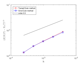
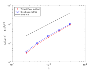
To detect the mean-square convergence rates, numerical approximations generated by the tamed (sine) Euler method with a fine stepsize $h=2^{-13}$ are used as the “exact” solutions for the order plots. Then other numerical approximations are calculated by (36) and (76) applied to (86) and (87), respectively, with five different stepsizes $h=2^{-i},i=8,9,10,11,12$. Here the expectations are approximated by the Monte Carlo approximation with $5000$ Brownian and Poisson paths.

Figure 1 shows that the slopes of the error lines and the reference lines match well, indicating that the proposed schemes have strong rates of order one-half in non-additive case and order one in additive case. Additionally, Table 1 lists the CPU time of numerical approximations by (36) and (76), generated by Matlab R2016a on a desktop (3.86 GB RAM, Intel(R) Core(TM) i5 CPU M480 at 2.67 GHz) with 64 bit Windows 7 operating system. It seems that the sine Euler method costs slightly less time than the tamed Euler method.

Figure 1. Mean-square convergence rates for (86) (left) and (87) (right)

Table 1: CPU time of the tamed and sine methods with different stepsizes
$h$	CPU time (second)
	non-additive case		additive case
	tamed method	sine method	tamed method	sine method
$2^{-8}$	0.869440	0.744448	0.794577	0.632519
$2^{-9}$	1.203300	0.932720	1.031226	0.776562
$2^{-10}$	1.625105	1.100245	1.276387	0.906966
$2^{-11}$	2.951017	1.887072	2.355608	1.433305
$2^{-12}$	5.789335	3.588197	4.325145	2.473830

Appendix A. Verification of assumptions for SDE examples.

In view of (86), the functions $f,g,\sigma\colon\mathbb{R}\to\mathbb{R}$ defined by $f(x)={\mu}x(\nu-|x|)$, $g(x)={\xi}|x|^{3/2}$ and $\sigma(x)={\eta}x\ln(1+x^{2})$ are continuous for all $x\in\mathbb{R}$. Then their derivatives are given by $f^{\prime}(x)={\mu}\nu-2{\mu}|x|$, $g^{\prime}(x)=\frac{3}{2}{\xi}\text{sgn}(x)|x|^{1/2}$ and $\sigma^{\prime}(x)=\eta(\tfrac{2x^{2}}{1+x^{2}}+\ln(1+x^{2}))$ for all $x\in\mathbb{R}$. The Appendix in [40] tells that

$$|f(x)-f(y)|^{2}\leq 3\mu^{2}\max\{1,\nu\}^{2}(1+|x|^{2}+|y|^{2})|x-y|^{2},\quad\forall x,y\in\mathbb{R},$$

which implies that Assumption 3.1 is satisfied with $q=2$. This together with Theorems 4.5 and 5.2 indicates that, for example, $\bar{p}=20\geq\max\{2+4H(q),2+2q\}$ is enough for our setting. To verify Assumption 2.1, we first use the mean value theorem and the Hölder inequality to get

$$\begin{split}&2\langle x-y,f(x)-f(y)\rangle+|g(x)-g(y)|^{2}+\int_{Z}|\sigma(x,z)-\sigma(y,z)|^{2}\,\nu(\mbox{d}z)\\ \leq&|x-y|^{2}\int_{0}^{1}\big{(}2f^{\prime}(u)+|g^{\prime}(u)|^{2}+\lambda|\sigma^{\prime}(u)|^{2}\big{)}\,\mbox{d}r,\quad\forall x,y\in\mathbb{R},\end{split}$$ (A.1)

where $u:=y+r(x-y)$. Then the inequality $\ln(1+x^{2})\leq 2|x|^{\frac{1}{2}}$ for all $x\in\mathbb{R}$ and (12) enable us to show

$$\begin{split}&2f^{\prime}(u)+|g^{\prime}(u)|^{2}+\lambda|\sigma^{\prime}(u)|^{2}\\ \leq&2{\mu}\nu-\big{(}4{\mu}-\tfrac{9}{4}{\xi}^{2}\big{)}|u|+2\lambda\eta^{2}\big{(}\tfrac{2u^{2}}{1+u^{2}}\big{)}^{2}+2\lambda\eta^{2}\big{(}\ln(1+u^{2})\big{)}^{2}\\ \leq&2{\mu}\nu+8\lambda\eta^{2}-\big{(}4{\mu}-\tfrac{9}{4}{\xi}^{2}-8\lambda\eta^{2}\big{)}|u|\leq 2{\mu}\nu+8\lambda\eta^{2},\end{split}$$ (A.2)

on the condition $4{\mu}-\tfrac{9}{4}{\xi}^{2}-8\lambda\eta^{2}>0$. Hence (A.1) and (A.2) prove (5) in Assumption 2.1 for $\mu=3,\nu=1,\xi=0.5,\eta=0.1,\lambda=1$. Similarly, we can show (6) as follows

$$\begin{split}&2\langle x,f(x)\rangle+|g(x)|^{2}+\int_{Z}|\sigma(x,z)|^{2}\,\nu(\mbox{d}z)\\ =&2{\mu}\nu|x|^{2}-\big{(}2{\mu}-{\xi}^{2}\big{)}|x|^{3}+\lambda{\eta}^{2}|x|^{2}(\ln(1+x^{2}))^{2}\\ \leq&2{\mu}\nu|x|^{2}-\big{(}2{\mu}-{\xi}^{2}-4\lambda{\eta}^{2}\big{)}|x|^{3}\leq 2{\mu}\nu(1+|x|^{2}),\quad\forall x\in\mathbb{R}^{d},\end{split}$$

as $2{\mu}-{\xi}^{2}-4\lambda{\eta}^{2}>0$. It remains to verify Assumption 2.3. Actually, recalling $\bar{p}=20$ and using the inequality $\ln(1+x^{2})\leq 200+|x|^{\frac{1}{\bar{p}}}$ for all $x\in\mathbb{R}$ and (12), we obtain, after taking $\varepsilon=1$,

$$\begin{split}&\bar{p}|x|^{\bar{p}-2}\langle x,f(x)\rangle+\tfrac{\bar{p}(\bar{p}-1)}{2}|x|^{\bar{p}-2}|g(x)|^{2}+\big{(}1+(\bar{p}-2)\big{)}\int_{Z}|\sigma(x,z)|^{\bar{p}}\,\nu(\mbox{d}z)\\ =&\bar{p}{\mu}\nu|x|^{\bar{p}}-\big{(}\bar{p}{\mu}-\tfrac{\bar{p}(\bar{p}-1)}{2}{\xi}^{2}\big{)}|x|^{\bar{p}+1}+\lambda\big{(}\bar{p}-1\big{)}{\eta}^{\bar{p}}|x|^{\bar{p}}(\ln(1+x^{2}))^{\bar{p}}\\ \leq&\big{(}\bar{p}{\mu}\nu+\lambda(\bar{p}-1)(400{\eta})^{\bar{p}}\big{)}|x|^{\bar{p}}-\big{(}\bar{p}{\mu}-\tfrac{\bar{p}(\bar{p}-1)}{2}{\xi}^{2}-\lambda(\bar{p}-1){(2\eta)}^{\bar{p}}\big{)}|x|^{\bar{p}+1}\\ \leq&\bar{p}{\mu}\nu(1+|x|^{\bar{p}}),\quad\forall x\in\mathbb{R}^{d},\end{split}$$

as $\bar{p}{\mu}\nu+\lambda(\bar{p}-1)(400{\eta})^{\bar{p}}>0$ and $\bar{p}{\mu}-\tfrac{\bar{p}(\bar{p}-1)}{2}{\xi}^{2}-\lambda(\bar{p}-1){(2\eta)}^{\bar{p}}>0$. Similarly, we can show that (87) fulfills Assumptions 2.1, 2.3 and 4.6 with $q=4$.

Received November 2017; 1st revision November 2018; 2nd revision March 2019.

References

- [1] A. Andersson and R. Kruse, Mean-square convergence of the BDF2-Maruyama and backward Euler schemes for SDE satisfying a global monotonicity condition, BIT Numer. Math., 57 (2017), 21–53.
- [2] D. Applebaum, Lévy Processes and Stochastic Calculus, Cambridge University Press, 2009.
- [3] W.-J. Beyn, E. Isaak and R. Kruse, Stochastic C-stability and B-consistency of explicit and implicit Euler-type schemes, J. Sci. Comput., 67 (2016), 955–987.
- [4] W.-J. Beyn, E. Isaak and R. Kruse, Stochastic C-stability and B-consistency of explicit and implicit Milstein-type schemes, J. Sci. Comput., 70 (2017), 1042–1077.
- [5] N. Bruti-Liberati and E. Platen, Strong approximations of stochastic differential equations with jumps, J. Comput. Appl. Math., 205 (2007), 982–1001.
- [6] K. Dareiotis, C. Kumar and S. Sabanis, On tamed Euler approximations of SDEs driven by Lévy noise with applications to delay equations, SIAM J. Numer. Anal., 54 (2016), 1840–1872.
- [7] S. Deng, W. Fei, W. Liu and X. Mao, The truncated EM method for stochastic differential equations with Poisson jumps, J. Comput. Appl. Math., 355 (2019), 232–257.
- [8] W. Fang and M. B. Giles, Adaptive Euler-Maruyama method for SDEs with non-globally Lipschitz drift: Part I, finite time interval, preprint, arXiv:1609.08101.
- [9] A. Gardoń, The order of approximation for solutions of Itô-type stochastic differential equations with jumps, Stoch. Anal. Appl., 22 (2004), 679–699.
- [10] I. Gyöngy and N. V. Krylov, On stochastic equations with respect to semimartingales I, Stoch., 4 (1980), 1–21.
- [11] D. J. Higham and P. E. Kloeden, Numerical methods for nonlinear stochastic differential equations with jumps, Numer. Math., 101 (2005), 101–119.
- [12] D. J. Higham, X. Mao and A. M. Stuart, Strong convergence of Euler-type methods for nonlinear stochastic differential equations, SIAM J. Numer. Anal., 40 (2002), 1041–1063.
- [13] D. J. Higham and P. E. Kloeden, Strong convergence rates for backward Euler on a class of nonlinear jump-diffusion problems, J. Comput. Appl. Math., 205 (2007), 949–956.
- [14] L. Hu and S. Gan, Convergence and stability of the balanced methods for stochastic differential equations with jumps, Int. J. Comput. Math., 88 (2011), 2089–2108.
- [15] M. Hutzenthaler and A. Jentzen, Convergence of the stochastic Euler scheme for locally Lipschitz coefficients, Found. Comput. Math., 11 (2011), 657–706.
- [16] M. Hutzenthaler and A. Jentzen, Numerical approximation of stochastic differential equations with non-globally Lipschitz continuous coefficients, Mem. Amer. Math. Soc., 236 (2015).
- [17] M. Hutzenthaler, A. Jentzen and P. E. Kloeden, Strong and weak divergence in finite time of Euler’s method for stochastic differential equations with non-globally Lipschitz continuous coefficients, Proc. R. Soc. A, 467 (2011), 1563–1576.
- [18] M. Hutzenthaler, A. Jentzen and P. E. Kloeden, Strong convergence of an explicit numerical method for SDEs with nonglobally Lipschitz coefficients, Ann. Appl. Probab., 22 (2012), 1611–1641.
- [19] M. Hutzenthaler and A. Jentzen, On a perturbation theory and on strong convergence rates for stochastic ordinary and partial differential equations with non-globally monotone coefficients, preprint, arXiv:1401.0295.
- [20] M. Hutzenthaler, A. Jentzen and X. Wang, Exponential integrability properties of numerical approximation processes for nonlinear stochastic differential equations, Math. Comp., 87 (2018), 1353–1413.
- [21] J. Jacod, T. G. Kurtz, S. Méléard and P. Protter, The approximate Euler method for Lévy driven stochastic differential equations, Ann. Inst. H. Poincaré–PR, 41 (2005), 523–558.
- [22] C. Kelly and G. J. Lord, Adaptive time-stepping strategies for nonlinear stochastic systems, IMA J. Numer. Anal., 38 (2018), 1523–1549.
- [23] P. E. Kloeden and E. Platen, Numerical Solution of Stochastic Differential Equations, Springer, Berlin, 1992.
- [24] A. Kohatsu-Higa and P. Tankov, Jump-adapted discretization schemes for Lévy-driven SDEs, Stoch. Proc. Appl., 120 (2010), 2258–2285.
- [25] C. Kumar and S. Sabanis, On explicit approximations for Lévy driven SDEs with super-linear diffusion coefficients, Electron. J. Probab., 22 (2017), Paper No. 73, 19 pp.
- [26] C. Kumar and S. Sabanis, On tamed Milstein schemes of SDEs driven by Lévy noise, Discrete Contin. Dyn. Syst. Ser. B, 22 (2017), 421–463.
- [27] W. Liu and X. Mao, Strong convergence of the stopped Euler-Maruyama method for nonlinear stochastic differential equations, Appl. Math. Comput., 223 (2013), 389–400.
- [28] X. Q. Liu and C. W. Li, Weak approximations and extrapolations of stochastic differential equations with jumps, SIAM J. Numer. Anal, 37 (2000), 1747–1767.
- [29] Y. Maghsoodi, Mean-square efficient numerical solution of jump-diffusion stochastic differential equations, Sankhy Ser. A., 58 (1996), 25–47.
- [30] X. Mao and L. Szpruch, Strong convergence and stability of implicit numerical methods for stochastic differential equations with non-globally Lipschitz continuous coefficients, J. Comput. Appl. Math., 238 (2013), 14–28.
- [31] X. Mao and L. Szpruch, Strong convergence rates for backward Euler-Maruyama method for non-linear dissipative-type stochastic differential equations with super-linear diffusion coefficients, Stoch., 85 (2013), 144–171.
- [32] X. Mao, The truncated Euler-Maruyama method for stochastic differential equations, J. Comput. Appl. Math., 290 (2015), 370–384.
- [33] X. Mao, Convergence rates of the truncated Euler-Maruyama method for stochastic differential equations, J. Comput. Appl. Math., 296 (2016), 362–375.
- [34] R. Mikulevicius and H. Pragarauskas, On -estimates of some singular integrals related to jump processes, SIAM J. Math. Anal., 44 (2012), 2305–2328.
- [35] G. N. Milstein, A theorem on the order of convergence of mean-square approximations of solutions of systems of stochastic differential equations, Tero. Prob. Appl., 32 (1987), 809–811.
- [36] G. N. Milstein and M. V. Tretyakov, Stochastic Numerics for Mathematical Physics, Springer, Berlin, 2004.
- [37] G. N. Milstein and M. V. Tretyakov, Numerical integration of stochastic differential equations with nonglobally Lipschitz coefficients, SIAM J. Numer. Anal., 43 (2005), 1139–1154.
- [38] E. Platen and N. Bruti-Liberati, Numerical Solution of Stochastic Differential Equations with Jumps in Finance, Springer-Verlag: Berlin, 2010.
- [39] P. Protter, Stochastic Integration and Differential Equations, A new approach, Springer-Verlag: Berlin-Heidelberg, 1990.
- [40] S. Sabanis, Euler approximations with varying coefficients: the case of super-linearly growing diffusion coefficients, Ann. Appl. Probab., 26 (2016), 2083–2105.
- [41] S. Sabanis, A note on tamed Euler approximations, Electron. Commun. Probab, 18 (2013), 1–10.
- [42] S. Sabanis and Y. Zhang, On explicit order 1.5 approximations with varying coefficients: the case of super-linear diffusion coefficients, J. Complexity, 50 (2019), 84–115.
- [43] Ł. Szpruch and X. Zhāng, -integrability, asymptotic stability and comparison property of explicit numerical schemes for non-linear SDEs, Math. Comp., 87 (2018), 755–783.
- [44] A. Tambue and J. D. Mukam, Strong convergence of the tamed and the semi-tamed Euler schemes for stochastic differential equations with jumps under non-global Lipschitz condition, preprint, arXiv:1510.04729.
- [45] M. V. Tretyakov and Z. Zhang, A fundamental mean-square convergence theorem for SDEs with locally Lipschitz coefficients and its applications, SIAM J. Numer. Anal., 51 (2013), 3135–3162.
- [46] X. Wang and S. Gan, Compensated stochastic theta methods for stochastic differential equations with jumps, Appl. Numer. Math., 60 (2010), 877–887.
- [47] X. Wang and S. Gan, The tamed Milstein method for commutative stochastic differential equations with non-globally Lipschitz continuous coefficients, J. Differ. Equ. Appl., 19 (2013), 466–490.
- [48] X. Yang and X. Wang, A transformed jump-adapted backward Euler method for jump-extended CIR and CEV models, Numer. Algor., 74 (2017), 39–57.
- [49] Z. Zhang and H. Ma, Order-preserving strong schemes for SDEs with locally Lipschitz coefficients, Appl. Numer. Math., 112 (2017), 1–16.
- [50] Z. Zhang, New explicit balanced schemes for SDEs with locally Lipschitz coefficients, preprint, arXiv: 1402.3708.
- [51] X. Zong, F. Wu and C. Huang, Convergence and stability of the semi-tamed Euler scheme for stochastic differential equations with non-Lipschitz continuous coefficients, Appl. Math. Comput., 228 (2014), 240–250.