Continuous cascades in the wavelet space as models for synthetic turbulence

Abstract

We introduce a wide family of stochastic processes that are obtained as sums of self-similar localized “waveforms” with multiplicative intensity in the spirit of the Richardson cascade picture of turbulence. We establish the convergence and the minimum regularity of our construction. We show that its continuous wavelet transform is characterized by stochastic self-similarity and multifractal scaling properties. This model constitutes a stationary, ”grid free”, extension of $\cal W$-cascades introduced in the past by Arneodo, Bacry and Muzy using wavelet orthogonal basis. Moreover our approach generically provides multifractal random functions that are not invariant by time reversal and therefore is able to account for skewed multifractal models and for the so-called “leverage effect”. In that respect, it can be well suited to providing synthetic turbulence models or to reproducing the main observed features of asset price fluctuations in financial markets.

I Introduction

The goal of modeling the observed “random” fluctuations of the velocity field and the intermittent character of the small scale dissipated energy in fully developed turbulent flows has played a critical role in the development of mathematical concepts around multifractal processes. In particular, random multiplicative cascades first considered by the Russian school Kolmogorov (1962); Obukhov (1962); Novikov and Stewart (1964) and subsequently developed by B. Mandelbrot Mandelbrot (1974a, b) in order to mimic the energy transfer from large to small scales Frisch (1995) represent the paradigm of multifractal random distributions. They are the basis of a lot of mathematical work and have led to a wide number of applications far beyond the field of turbulence.

Mandelbrot cascades ($\cal M$-cascades) mainly consist in building a random measure by using a multiplicative iterative rule. One starts with some large interval with a constant measure density $W_{0}$ and splits this interval in two equal parts. The measure density in the left and right half parts are obtained by multiplying $W_{0}$ by respectively two independent, identically distributed positive factors (say $W_{1}^{L}$ and $W_{1}^{R}$). This operation is then repeated independently on the two sub-intervals and so on, ad infinitum, in order to converge towards a singular measure which properties have been studied extensively (see e.g. Mandelbrot (1974b); Kahane and Peyrière (1976); Guivarc’h (1987); Barral (2004)). The main disadvantage of $\cal M$-cascades is that they involve a specific scale ratio ($s=2$ in general) and are limited to live in the starting interval. This lack of stationarity and continuous scale invariance is obviously not suited to accounting for natural phenomena. In order to circumvent these problems, continuous extensions of Mandelbrot cascades were proposed by first Barral and Mandelbrot Barral and Mandelbrot (2002) and later by Bacry and Muzy Muzy and Bacry (2002); Bacry and Muzy (2003). The idea under these constructions is to replace the discrete multiplicative density $\prod_{i=1}^{n}W_{i}=e^{\sum_{i=1}^{n}\ln W_{i}}$ by $e^{\omega_{\ell}(t)}$ where $\omega_{\ell}(t)$ is an infinitely divisible noise chosen with a logarithmic correlation function designed to mimic the tree-like (in general a dyadic tree) structure underlying $\cal M$-cascades Arneodo et al. (1998a); Muzy et al. (2000); Schmitt, F. and Marsan, D. (2001).

The above definitions of random cascade measures led to a large number of extensions notably in order to construct stochastic processes with some predefined regularity properties. The most popular approach was initiated by Mandelbrot (see e.g. Mandelbrot et al. (1997)) and consists in compounding a self-similar stochastic process like the (fractional-) Brownian motion $B_{H}(t)$ with a “multifractal time” $M(t)$, a multifractal measure of the interval $[0,t]$ as provided by a continuous cascade. Such a compounded process $B_{H}(M(t))$ inherits the multifractal scaling properties of $M(t)$ with a ”main” regularity that corresponds to the self-similar process $B_{H}(t)$. An alternative but related approach, was initially proposed with the construction of “the Multifractal Random Walk” (MRW) in Muzy et al. (2000); Bacry et al. (2001) and that consists of interpreting $M(dt)$ as the local variance of a fractional Brownian motion $B_{H}(t)$. As emphasized in Muzy and Bacry (2002); Ludena (2008); P. Abry and Pipiras (2009), this amounts to constructing a multifractal process as (the limit of) a stochastic integral like $\int e^{\omega_{\ell}(t)}dB_{H}(t)$. This point of view is inspired from classical stochastic volatility models of financial markets that aim at accounting for the observed bursts in price fluctuations by the random nature of the variance of an underlying Gaussian law. It can also be understood as a formalization of the so-called ”Kolmogorov refined similarity hypothesis” Frisch (1995) according to which the velocity fluctuation $\delta v$ and the local rate of dissipated energy $\varepsilon$ are related as, in its Lagrangian version Benzi et al. (2009), $\delta_{\tau}v\sim\varepsilon_{\tau}^{1/2} dW_{\tau}$, $dW_{\tau}$ being a noise such that $\mathbb{E}\left[dW_{\tau}^{2}\right]=\tau$. Accordingly, the multifractal properties of the velocity field directly come from those of the local dissipation field $\varepsilon$, a multifractal cascade interpreted as a “local variance”. The main advantage of continuous cascades and their associated random processes is that they provide a large class of parsimonious models with stationary increments and continuous stochastic scale invariance properties. From a practical point of view, they are easy to calibrate from data and can provide simple analytical or numerical solutions to many statistical problems. However, the aforementioned methods to derive a multifractal process from a multifractal measure lack of flexibility and in particular hardly allow one to describe processes that are not invariant by time reversal. This means that the increment distribution skewness (i.e. non vanishing third order moments of the increments at different scales) as observed in turbulence or the leverage effect (i.e. some causal, asymmetric relationship between increment signs and increment amplitudes) as observed in financial time series cannot be captured easily within this framework. All former attempts to address this issue were based on studying a random noise like $e^{\omega_{\ell}(t)}\Delta B_{H}(t)$ for a specific cross-covariance between $\omega_{\ell}$ and $\Delta B_{H}$ Pochart and Bouchaud (2002); Bacry et al. (2012). However, as discussed in Bacry et al. (2012), this approach leads to a non degenerated limiting process only in some restricted range $H>1/2$ and therefore cannot be used as a model for financial markets ($H\simeq 1/2$) or turbulence ($H\simeq 1/3$). More recently, Chevillard et al. Chevillard et al. (2017a) introduced a new model which obeys to multifractal scaling with a (signed) third order structure function that behaves as a linear function, like in turbulence. This model is defined within the context of Gaussian Multiplicative Chaos (i.e. a Gaussian version of $\omega_{\ell}(t)$) and mainly consists in considering a fractional integration of a product like $\omega^{\prime}e^{\omega}dB$ where $\omega^{\prime}$ represents a peculiar intermittent version of $\omega$, independent of $\omega$ but correlated with the white noise $dB$. The authors have shown that their construction leads to a properly defined intermittent skewed random process. However, we can point out that the model of Chevillard et al. is far from being simple, involves cumbersome computations and is not characterized by self-similar properties, it follows a multifractal scaling only in the limit of small scales.

In this paper, we propose a different path to solve the challenging issue of mixing multiscaling properties and non-invariance by time reversal. Beyond this question, our construction also offers an appealing alternative way to build a large class of multifractal functions with well controlled scaling (or regularity) properties and that are characterized by new features as compared to former constructions. Our approach is directly inspired from the random cascade picture originally proposed by Richardson Richardson (1922) under which, in turbulent flows, large eddies are stretched and broken into smaller ones to which they transfer a fraction of their energy and so on, up to the dissipation scale. Instead of trying to capture the velocity field intermittency from the final state of such a cascade, i.e., the dissipation field (which is a multifractal measure), the previous scenario suggests that one could describe the overall flow as a superposition of coexisting structures at all scales correlated with each other by a cascading intensity (energy). This viewpoint of decomposing a function as a weighted sum of waveforms (the ”eddies”) at different scales precisely corresponds to a wavelet transform representation Mallat (1999). The construction of discrete multiplicative cascades along the wavelet tree associated with orthogonal wavelet basis has been already proposed two decades ago by Arneodo, Bacry and Muzy Arneodo et al. (1998b). These ”$\cal W$-cascades” have proven to be an appealing alternative to $\cal M$-cascade based constructions in order to directly build multifractal stochastic processes Arneodo et al. (1998a); Barral and Seuret (2005). They also provided a suitable approach to extent the framework of stochastic self-similarity and build new random functions with a non trivial spectrum of oscillating singularities Arneodo et al. (1997a, 1998c). Our goal in this paper is thus to construct an extension of $\cal W$-cascades in order to get rid of the restraining grid structure of wavelet orthogonal basis that prevent, very much like grid-bounded $\cal M$-cascades, $\cal W$-cascades from being able to simply account for stationarity and continuous scale invariance. For that purpose, we just consider a continuous sum over space $t$ and scales $\ell$ of “sythetizing wavelets” weighted by a factor that is precisely given by the stochastic density involved in continuous cascades, $e^{\omega_{\ell}(t)}$. We show that such a construction allows us to obtain well defined processes with a large flexibility on their scaling and regularity properties. Moreover it generically leads to skewed processes and is able to reproduce the leverage effect for specific shapes of synthetizing wavelets. In that respect, they can naturally be invoked as models for synthetic turbulence or calibrated to account for asset fluctuations in financial markets. Various numerical examples are provided throughout the paper in order to illustrate our purpose and notably to show the model ability to reproduce many of the observed features of the longitudinal velocity field fully developed turbulence experiments.

The paper is structured as follows: in section II we recall the main lines of continuous cascades (Sec. II.1) and $\cal W$-cascades (Sec. II.2) constructions. This notably allows us to introduce the process $\omega_{\ell}(t)$ and review its main statistical properties. Our new constrution of continuous cascades in the wavelet plane ($\cal CW$-cascades) are introduced in section III. After the definition and the statement of a weak convergence result, we provide some numerical examples (Sec. III.1). In Sec. III.2, we study their wavelet transform and establish the almost sure minimum regularity of their paths. Scaling and self-similarity properties of this new class of processes are studied in section IV. We prove that their structure functions are characterized by a power-law behavior with some non-linear $\zeta_{q}$ spectrum of scaling exponents (Sec. IV.1) and study the correlation functions of the absolute increments (Sec. IV.2). We finally study the properties of $\cal CW$-cascades as respect to time reversal, notably the behavior of the skewness and the leverage function (Sec. V). Concluding remarks and prospects for future research are given in section VI  while technical material and proofs are provided in appendices.

II Continuous cascades and $\cal W$-cascades

This section contains a brief review of the notions of “continuous” and “wavelet” multiplicative cascades. The first ones were introduced as stationary, self-similar singular measures with log-infinitely divisible multifractal properties while $\cal W$-cascades are the wavelet transform counterparts of Mandelbrot discrete multiplicative cascades. As explained in Sec. III, both constructions will be mixed in order to build continuous wavelet cascade models.

II.1 Log-infinitely divisible continuous cascades

Continuous random cascades are stochastic measures $M(t)$ introduced few years ago (Bacry et al. (2001); Schmitt and Marsan (2001); Barral and Mandelbrot (2002); Muzy and Bacry (2002); Bacry and Muzy (2003)) in order to extend, within a stationary and grid-free framework, the Mandelbrot discrete multiplicative cascades. Such a measure $M(t)=\int_{0}^{t}dM_{u}$ can have exact multifractal scaling properties in the sense that it satisfies, for a given $T>0$, $\forall t\leq T$:

$$\mathbb{E}\left[M(t)^{q}\right]=K_{q}\left(\frac{t}{T}\right)^{\zeta_{q}}$$ (1)

where $\zeta_{q}$ is a non-linear concave function called the multifractal spectrum (or the spectrum of structure functions scaling exponents in the context of turbulence Frisch (1995); Arneodo et al. (1996)) and $K_{q}$ is a (eventually infinite) prefactor corresponding the the $q$-order moment at scale $t=T$.

In Muzy and Bacry (2002); Bacry and Muzy (2003) (see also Barral and Mandelbrot (2002)) $dM(t)$ is obtained as the (weak) limit, when $\ell\to 0$ of the measure with density:

$$dM_{\ell}(t)=e^{\omega_{\ell}(t)}dt$$ (2)

where $e^{\omega_{\ell}(t)}$ is a stationary log-infinitely divisible process representing the continuous cascade from scale $T$ to scale $\ell$. Its precise definition and main properties, reviewed in Appendix A, notably imply that it satisfies (thanks to Eqs. (49) and (50)):

$$\mathbb{E}\left[e^{q\omega_{\ell}(t)}\right]=\left(\frac{T}{\ell}\right)^{\phi(q)}$$ (3)

where $\phi(q)$ is the cumulant generating function associated with an infinitely divisible law as provided by the celebrated Levy-Khintchine Theorem Feller (1971). Moreover, $\omega_{\ell}(t)$ verifies, $\forall s<1,u\in[0,T]$,

$$\omega_{s\ell}(su)\stackrel{{\scriptstyle\cal L}}{{=}}\Omega_{s}+\omega_{\ell}(u)$$ (4)

where $\stackrel{{\scriptstyle\cal L}}{{=}}$ means that the two processes have the same finite dimensional distributions of any order and $\Omega_{s}$ is a random variable independent of the process $\omega_{\ell}(t)$ with the same distribution as $\omega_{sT}(t)$. The multifractal scaling (1) follows since Eq. (4) entails

$$M(st_{0})=\lim_{\ell\to 0}\int_{0}^{st_{0}}e^{\omega_{s\ell}(u)}du\stackrel{{\scriptstyle\cal L}}{{=}}se^{\Omega_{s}}\lim_{\ell\to 0}\int_{0}^{t_{0}}e^{\omega_{\ell}(u)}du=se^{\Omega_{s}}M(t_{0})$$ (5)

and thus by choosing $t_{0}=T$ and $s=t/T$, we have

$$\mathbb{E}\left[M(t)^{q}\right]=s^{q}\mathbb{E}\left[e^{q\Omega_{s}}\right]\mathbb{E}\left[M(T)^{q}\right]$$

that leads, using Eq. (3), to Eq. (1) with

$$\zeta_{q}=q-\phi(q)\;.$$

As discussed in the introduction, a large class of multifractal processes $X(t)$ with stationary increments can be obtained from a multifractal measure $M(t)$. One can, as suggested by Mandelbrot Mandelbrot et al. (1997); Mandelbrot (1999), compound a self-similar process $B_{H}(t)$ (e.g., a fractional Brownian motion) by the non-decreasing function $M(t)$ so that:

$$X(t)=B_{H}(M(t))\;.$$

Within this approach $M(t)$ is referred to as the ”multifractal time”. Since $B_{H}(st)\stackrel{{\scriptstyle\cal L}}{{=}}s^{H}B_{H}(t)$, one has

$$X(st)\stackrel{{\scriptstyle\cal L}}{{=}}s^{H}e^{H\Omega_{s}}X(t)$$

that entails, given the increment stationarity of $X(t)$, the multiscaling of the structure functions:

$$\mathbb{E}\left[|X(t+\tau)-X(t)|^{q}\right]=C_{q}\tau^{\zeta_{q}}$$

with $\zeta_{q}=qH-\phi(qH)$. Another approach initiated in Muzy et al. (2000); Bacry et al. (2001) (see also Muzy and Bacry (2002)) is to consider the limit $\ell\to 0$ of the sequence $X_{\ell}(t)=\sum_{k=1}^{t/\ell}\ell^{\alpha}e^{\omega_{\ell}(k)}dW_{k}$ where $dW_{k}$ is a fractional Gaussian noise and $\alpha$ an appropriate constant chosen to ensure the convergence (in some specific sense) of the series. This amounts to interpreting $e^{\omega_{\ell}(k)}$ as a stochastic variance or, in the field of mathematical finance, a ”stochastic volatility”. Related constructions consist in considering stochastic integrals like $\int e^{\omega_{\ell}(t)}dB_{H}(t)$, where $B_{H}(t)$ is a fractional Brownian motion Muzy and Bacry (2002); Ludena (2008); P. Abry and Pipiras (2009). All these approaches were extensively used and studied in the literature as paradigms of multifractal processes satisfying exact stochastic scale-invariance properties and also considered as toy models for applications like turbulence or financial time series. However, as recalled in the introduction, they mainly involve separately the construction of a multifractal measure and a self-similar process and do not consist in directly building the random process $X(t)$ with some specific properties. It then results a lack of flexibility in the obtained features, in particular, as emphasized previously and discussed in Pochart and Bouchaud (2002); Bacry et al. (2012); Chevillard et al. (2017a), skewed statistics and ”leverage effect” cannot be obtained in a fully satisfactory way through these approaches. As reviewed below, wavelet cascades offer an interesting alternative in the sense that they do not rely on any preset self-similar process and consists in directly building $X(t)$ with a control of its scaling or regularity properties.

II.2 $\cal W$-cascades

In Ref. Arneodo et al. (1998b), the authors introduced the so-called $\cal W$-cascades as the natural transposition of Mandelbrot $\cal M$-cascades within the framework a orthogonal wavelet transform. This allows one to construct multifractal processes or distributions with a precise control of their regularity properties. The idea is to build a new class of (multi-)fractal functions $Z(t)$ from their explicit representation over a wavelet basis:

$$Z(t)=\sum_{j=0}^{\infty}\sum_{k=0}^{2^{j-1}}c_{j,k}\psi_{j,k}(t)$$ (6)

where $\psi_{j,k}(t)=2^{j}\psi(2^{j}t-k)$ and $\{\psi_{j,k}(t)\}_{j,k\in\mathbb{Z}}$ constitutes an orthogonal wavelet basis of the interval. The wavelet coefficients $c_{j,k}=\int Z(u)\psi_{j,k}(u)du$ are chosen according to the multiplicative cascade rule Arneodo et al. (1998b):

$$c_{j,2k}=W_{0}\;c_{j-1,k},\;\;c_{j,2k+1}=W_{1}\;c_{j-1,k}$$ (7)

with $W_{0}$ and $W_{1}$ are i.i.d. copies of a real valued random variable $W$. We see that, if $W$ is a positive random variable, the law of the wavelet coefficient $c_{j,k}$ is precisely given by the law of the density of a $\cal M$-cascade at construction step $j$:

$$c_{j,k}=\prod_{m=0}^{j}W_{m}$$ (8)

It has been shown in Arneodo et al. (1998b) that, under some mild condition on the law of $W$, $Z(t)$ is a well defined multifractal process with almost surely Lipschitz regular paths. Such a construction of multifractal functions associated with specific random wavelet series has been extended recently by Barral and Seuret Barral and Seuret (2005). If $M$ stands for a Mandelbrot multifractal measure (a $\cal M$-cascade) constructed from an iterative random multiplicative rule as described in the introduction, these authors considered a wavelet random series like (6) but where $c_{j,k}$ is given by the measure of the associated dyadic interval $I_{j,k}=[k2^{-j},(k+1)2^{-j}]$:

$$c_{j,k}=2^{-j\alpha}M(I_{j,k})\;.$$

Barral and Seuret proved that the scaling and regularity properties of $Z(t)$ are directly inherited from those of $M(t)$. Moreover, they have shown that, under specific conditions, replacing $\prod_{i=1}^{j}W_{i}$ of $\cal W$-cascades by the limit measure of the associated dyadic interval, $M(I_{j,k})$ does not change the multifractal properties (see the Sec. IV.1 for more details).

Unlike the constructions of multifractal processes based on multifractal measures, $\cal W$-cascades allow one to directly build multifractal processes without the need for any additional self-similar process. However, very much like $\cal M$-cascades, they do involve a dyadic tree and a finite time interval that can hardly be used to fit most of experimental situations. For that reason, in the same manner as $\cal M$-cascades have been extended to log-infinitely divisible continuous cascades, we aim at defining a continuous version of $\cal W$-cascades.

III Continuous $\cal W$-cascades

In this section, we introduce the new class of models we consider in the paper. Our goal is to extend the previously described $\cal W$-cascades to a grid-free background. The main idea is to replace the discrete sum (6) by a continuous sum over space and scales and the discrete product in Eq. (8) at scale $\ell=2^{-j}$ by its “continuous” (i.e. stationary and ”grid free”) counterpart $e^{\omega_{\ell}(t)}$ described in Sec. II.1 and Appendix A.

III.1 Definition and numerical illustrations

III.1.1 Definition and convergence

Let us define a stochastic process $X(t)$ as a (continuous) sum of localized waveforms (i.e. ”wavelets”) of size $\ell$ and which intensity is given by the class of stationary, log-infinitely divisible process $e^{\omega_{\ell}(t)}$ used in the definition of continuous cascades of Section II.1.

Let $H>0$, $\ell>0$ and consider the following (well defined) integral:

$$X_{\ell}(t)=\int_{\ell}^{T}\!s^{H-2}ds\!\int_{-\infty}^{+\infty}e^{\omega_{s}(b)}\varphi\left(\frac{t-b}{s}\right)db$$ (9)

where $\omega_{s}(u)$ is the infinitely divisible process defined in Section II.1 and $\varphi(t)$ is a wavelet that can be chosen as a square integrable smooth function with compact support (e.g, the interval $[-{1\over 2},{1\over 2}]$) and which is sufficiently oscillating so that its first $N$ moments vanish. Hereafter, we will referred to this wavelet as the “synthetizing wavelet”. As emphasized below, this amounts, in some sense, to interpreting $s^{H}e^{\omega_{\ell}(t)}$ as the continuous wavelet transform of $X(t)$ at time $t$ and scale $\ell$, Eq. (9) corresponding to the continous wavelet reconstruction formula. Let us remark that, if $\phi(1)<\infty$, one can, without loss of generality (since it simply consists in redefining the parameter $H$), always assume that in Eq. (9), $\omega_{s}(t)$ is chosen such that

$$\mathbb{E}\left[e^{\omega_{s}(t)}\right]=1\Leftrightarrow\phi(1)=0\;.$$ (10)

In Appendix B, we establish the weak convergence of $X_{\ell}(t)$ in the space of continuous functions when $\ell\to 0$. Namely, we show that the weak limit

$$\lim_{\ell\to 0}X_{\ell}(t)=X(t)$$ (11)

exists as a continuous function provided:

$$H>\frac{\phi(2)}{2}\;.$$ (12)

We will call such a limit $X(t)$ a “continuous wavelet cascade” process or a ${\cal CW}$-cascade. Let us notice that the condition (12) is precisely the analog of the condition for $L^{2}$ convergence of $\cal W$-cascades established by Arneodo et al. (condition $H1$ of Proposition 1 in Arneodo et al. (1998b)).

Figure 1: Examples of synthetizing wavelets $\varphi(t)$. (a) The compactly supported odd function $h^{(2)}(t)$ (Eq. (14)). (b) The ”Mexican hat”, i.e. the even wavelet $g^{(2)}(t)$ (Eq. (15)). (c) A non symmetric wavelet obtained by smoothing an asymmetric version of the Haar wavelet.

Figure 2: Sample paths of continuous log-normal $\cal W$-cascades $X(t)$ corresponding to 3 different values of the parameter $H$. In all cases, the intermittency coefficient and the integral scale were chosen to be respectively $\lambda^{2}=0.025$ and $T=1024$ and the synthetizing wavelet the $C^{2}$ version of the Haar wavelet, $h^{(3)}(t)$.

III.1.2 Numerical examples

In numerical experiments, one has to choose the infinitely divisible law of the process $\omega_{\ell}(t)$, the regularity parameter $H$, the integral scale $T$ and the synthetizing wavelet $\varphi(t)$. The simulation procedure simply consists in a discretization of Eq. (9). Its main lines are described in Appendix D.

All the examples provided in the paper are involving log-normal cascades which are the simplest ones to handle and that involve a single variance parameter $\lambda^{2}$. This means that $\omega_{\ell}(t)$ is a Gaussian process with a covariance function given by expression (49). In that respect, thanks to condition (10), the function $\phi(q)$ simply reads:

$$\phi(q)=\frac{\lambda^{2}}{2}q(q-1)\;.$$ (13)

and the condition (12) simply becomes $\lambda^{2}<2H$. Let us remark that this condition appears to be less restrictive than the condition of existence of a MRW $\lambda^{2}<1/2$ Bacry et al. (2001); Delour (2001) and it is a priori possible to build ${\cal CW}$-cascades with a large intermittency coefficient.

Among the choices we made for the synthetizing wavelets $\varphi$ there is the class of smooth variants of the Haar wavelet:

$$h^{(n)}(t)=\left(\mathbb{I}\underset{n}{\star\ldots\star}\mathbb{I}\star h\right)(t)$$ (14)

where $\mathbb{I}(t)$ is the indicator function of the interval $[0,1/2)$, $h(t)=\mathbb{I}(t+1/2)-\mathbb{I}(t)$ is the Haar wavelet and $\star$ stands for the convolution product. Notice that $h^{(n)}(t)$ has one vanishing moment and is of class $C^{n-1}(\mathbb{R})$. We also use wavelets in the class of the derivatives of the Gaussian function:

$$g^{(n)}(t)=\frac{d^{n}}{dt^{n}}e^{-\frac{x^{2}}{2}}\;.$$ (15)

Some examples among these wavelet classes are plotted in Fig. 1 (dilation and normalization factors are arbitrary). Note that one can also consider asymmetric wavelets as the one illustrated in the right panel of Fig. 1 that is contructed by asymmetrizing and smoothing the Haar wavelet (see Sec. V for an usage of asymmetric wavelets).

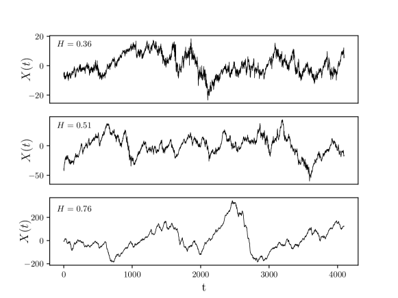
Some examples of sample paths of $X(t)$ are plotted in Figs. 2. All processes were generated using a Gaussian process $\omega_{\ell}(t)$ with the intermittency coefficient $\lambda^{2}=0.025$ and the integral scale $T=2048$. The synthetizing function was chosen to be $\varphi(t)=h^{(3)}(t)$. The scaling parameter $H$ has been chosen to be respectively $H=0.36$, $H=0.51$ and $H=0.76$ from top to bottom. One can see that $H$ directly controls the global regularity of the paths, the larger $H$, the more regular the path of $X(t)$ is. This is the analog of the parameter $H$ of the fractional Brownian motion Taqqu and Samorodnisky (1994). It is noteworthy that despite $X(t)$ appears to be a process with zero mean stationary increments, unlike all constructions proposed so far for mulifractal stationary processes, it does not involve any supplementary ”white” or ”colored” noise, like the Gaussian white noise, since it is only based on the ”intensity” process $e^{\omega_{\ell}(t)}$ as a source of randomness (see the remark at the end of the next section).

III.2 Wavelet transform, global regularity and reconstruction formula

In order to study and characterize the limiting process $X(t)$, one can compute its wavelet transform Mallat (1999). If $\psi(t)$ stands for some analyzing wavelet, let us introduce the kernel $K_{\varphi,\psi}(x,s)$ defined as:

$$K_{\varphi,\psi}(x,s)=s^{-1}\int\varphi\left(t\right)\psi\left(\frac{t-x}{s}\right)dt\;.$$ (16)

The wavelet transform of $X(t)$ can then be simply expressed as:

$$W(x,a)=a^{-1}\int X(t)\psi\left(\frac{t-x}{a}\right)dt=\int_{0}^{T}s^{H-2}ds\!\!\int_{-\infty}^{+\infty}db\;e^{\omega_{s}(b)}K_{\varphi,\psi}\left(\frac{x-b}{s},\frac{a}{s}\right)$$ (17)

It is easy to show that if $\psi$ has more than $N$ vanishing moments one has $K_{\varphi,\psi}(x,s)\sim s^{N}$ when $s\ll 1$ while if $\varphi$ has also at least $N$ vanishing moments, then $K_{\varphi,\psi}(x,s)\sim s^{-(N+1)}$ when $s\gg 1$. In that respect, for each $x$, $K_{\varphi,\psi}(x,s)$ is maximum around $s=1$. Moreover, if $\psi$ is also supported by $[-1/2,1/2]$, then $K(x,s)=0$ if $|x|\geq s$. In the sequel, for the sake of simplicity and to avoid cumbersome considerations about the tails of $K(x,s)$ for large and small $s$, we will suppose that the kernel $K(x,s)$ is non vanishing only in the time-scale interval $s\in[\kappa s,1]$, $x\in[-s,s]$ for some $\kappa<1$. Under this assumption, the wavelet transform of $X(t)$ can be approximated as:

$$W(x,a)\simeq\left\{\begin{array}[]{ll}&\!\!\!\int\limits_{\kappa a}^{\min(T,a)}s^{H-2}ds\int\limits_{x-a}^{x+a}e^{\omega_{s}(b)}K_{\varphi,\psi}\left(\frac{x-b}{s},\frac{a}{s}\right)db,\;\;\mbox{if}\;\kappa a\leq T\\ &0\;\;\mbox{otherwise}\end{array}\right.$$ (18)

Let us remark that in the case one chooses the analyzing wavelet $\psi(t)=\delta^{(1)}(t)$ with

$$\delta^{(1)}(t)=\delta(t+1)-\delta(t),$$ (19)

where $\delta(t)dt$ stands for the Dirac distribution, then $W(t,a)$ is nothing but the increment of $X(t)$ at scale $a$ Muzy et al. (1993):

$$W(t,a)=\delta_{a}X(t)=X(t+a)-X(t)$$ (20)

Despite this ”poor man’s wavelet” does not possess the requested regularity and oscillating properties (in particular approximation (18) is not supposed to hold), in the sequel, we will often consider that the increments statistics can be deduced from the wavelet transform statistics as a particular case (see e.g. Muzy et al. (1993) for a discussion on this specific topic). Along the same line, if $\psi(t)=\delta^{(2)}(t)$, with

$$\delta^{(2)}(t)=\delta(t+2)+\delta(t)-2\delta(t+1)$$ (21)

then $W(t,a)$ corresponds to the increments of second order of $X(t)$: $W(t,a)=X(t+2a)+X(t)-2X(t+a)$. Hereafter, we will refer to increments of first or second order when it is necessary to distinguish these two specific types of wavelet transforms.

Let us define the spectrum of structure function scaling exponents

$$\zeta_{q}=qH-\phi(q)$$ (22)

and consider its Legendre transform:

$$F(h)=1+\inf_{q}(qh-\zeta_{q})\;.$$ (23)

Let us suppose that $\exists\eta>0$ such that $F(h)<0$ for all $0\leq z<\eta$. In Appendix B, we use expression (18) to show that, for any $L>0$, almost surely, the paths of $X(t)$ have a uniform Lipschitz regularity $\alpha$ on $[0,L]$ for all $0<\alpha<h_{\min}$ with

$$h_{\min}=\arg\max\{F(h)<0\}_{h<H-\phi^{\prime}(0)}\;.$$

This result about the almost sure regularity of the paths $X(t)$ extends to continuous $\cal W$-cascades a similar property proven by Arneodo et al. in the case of discrete $\cal W$-cascades Arneodo et al. (1998b). For example, in the log-normal case, $\phi(q)$ is provided in Eq. (13) and therefore $h_{0}=H-\phi^{\prime}(0)=H+\frac{\lambda^{2}}{2}$. Since $F(h)=1-\frac{(h-h_{0})^{2}}{2\lambda^{2}}$, we obtain, provided $H>\sqrt{2\lambda^{2}}-\frac{\lambda^{2}}{2}$, i.e., $h_{\min}=h_{0}-\sqrt{2\lambda^{2}}>0$.

Let us notice that, unlike discrete $\cal W$-cascades, the weighting process $s^{H}e^{\omega_{\ell}(t)}$ involved in the continuous version is always positive. Nevertheless, let us remark that wavelet analysis is also helpful to show that, in the construction (9), instead of choosing the (positive) weights $s^{H}e^{\omega_{s}(b)}$, one could equivalently build $X(t)$ from a zero mean weighting process that has the same law as $W(b,s)$, the wavelet transform of $X(t)$. Indeed, let us consider the following process:

$$X^{\prime}(t)=\lim_{\ell\to 0}\lim_{R\to\infty}\int_{\ell}^{R}ds\;s^{-2}\!\int_{-\infty}^{+\infty}W(b,s)\varphi\left(\frac{t-b}{s}\right)db$$ (24)

where $W(b,s)$ is the wavelet transform of $X(t)$ as defined in (17). According to the wavelet point-wise reconstruction formula (e.g. as introduced in Holschneider and Tchamitchian (1991)), if the analyzing wavelet $\psi$ satisfies some mild conditions as respect to the synthetizing wavelet $\varphi$, one expects that $X^{\prime}(t)=X(t)$ at every point of continuity of $X(t)$. It thus results that (24) provides a whole family of versions of continuous $\cal W$-cascades contruction were the weights are chosen to be a zero mean process as simply obtained from any wavelet transform of the original $X(t)$ function.

IV Self-similarity and scaling properties

In this section we study the scaling and self-similarity properties of $X(t)$ as defined in Eqs. (9) and (11).

IV.1 Stochastic self-similarity of the wavelet transform. Multifractal Scaling

Let us first point out that, from the construction of $\omega_{\ell}$ as recalled in Appendix A, Eq. (50) can be naturally generalized as:

$$\mathbb{E}\left[e^{\sum_{m=1}^{q}ip_{m}\omega_{\ell_{m}}(x_{m})}\right]=e^{\sum_{j=1}^{q}\sum_{k=1}^{j}\alpha(j,k)\rho_{\max(\ell_{k},\ell_{j})}(x_{k}-x_{j})}$$ (25)

for any sequence $0,\ell_{1},\ldots,\ell_{q}<T$. From the expression (49) of $\rho_{\ell}(t)$, it results that Eq. (4) can be extended as equality in law for processes of both space and scale variables: one has, $\forall r<1$, $0<\ell\leq T$ and $u\in[0,T]$,

$$\omega_{r\ell}(su)\stackrel{{\scriptstyle\cal L^{\prime}}}{{=}}\Omega_{r}+\omega_{\ell}(u)$$ (26)

where where $\stackrel{{\scriptstyle\cal L^{\prime}}}{{=}}$ means that the two processes have the same finite dimensional distributions of any order as processes in the half-plane $(\ell,u)$ and $\Omega_{r}$ is a random variable of same law as $\omega_{rT}(u)$ independent of the process $\omega_{\ell}(t)$.

Let $r<1$ and $a\ll T$. From Eq. (18), the rescaled version of the wavelet transform of $X(t)$ reads:

$$W(rx,ra) \simeq \int\limits_{\kappa ra}^{ra}s^{H-2}ds\int\limits_{rx-ra}^{rx+ra}e^{\omega_{s}(b)}K_{\varphi,\psi}\left(\frac{rx-b}{s},\frac{ra}{s}\right)db$$

$$= r^{H}\int\limits_{\kappa a}^{a}s^{H-2}ds\int\limits_{x-a}^{x+a}e^{\omega_{rs}(rb)}K_{\varphi,\psi}\left(\frac{x-b}{s},\frac{a}{s}\right)db\;.$$

Thanks to Eq. (26), we can thus establish the self-similarity of the wavelet transform of $X(t)$:

$$W(rx,ra)\stackrel{{\scriptstyle{\cal L^{\prime}}}}{{=}}r^{H}e^{\Omega_{r}}W(x,a)\;.$$ (27)

Figure 3: Power-law scaling of structure functions of $X(t)$. In the top panel the structure function $S(q,a)$ of $X(t,a)$ (with $H=0.36$) are plotted in double logarithmic scale for $q=1,2,3,4$. The scaling behavior holds up to $a\simeq 2.10^{3}$ which corresponds to the integral scale $T$. In the bottom panel, the estimated $\zeta_{q}$ ($\circ$) are compared to the expected log-normal expressions as given by Eq. (31) (dashed lines) for $H=0.36$, $0.52$ and $0.77$ and $\lambda^{2}=0.025$.

From Eq. (27), the definition of $\Omega_{r}$ , Eqs. (3) and (22) it results that, for all $a\leq T$, the wavelet structure functions are characterized by the multifractal scaling:

$$S(q,a)=\mathbb{E}\left[|W(x,a)|^{q}\right]=C_{q}\left(\frac{a}{T}\right)^{qH-\phi(q)}=C_{q}a^{\zeta_{q}}\;,$$ (28)

where $C_{q}=\mathbb{E}\left[|W(x,T)|^{q}\right]$. $X(t)$ has therefore multifractal properties in the sense that the absolute moments of its wavelet transform behave has a power-law with a non-linear concave multifractal spectrum $\zeta_{q}$ Muzy et al. (1991, 1993). In particular, by considering Eq. (20), we deduce that the moments of absolute increments behave has power-laws with the multifractal spectrum $\zeta_{q}$:

$$\mathbb{E}\left[|X(t+a)-X(t)|^{q}\right]=C_{q}a^{\zeta_{q}}\;.$$ (29)

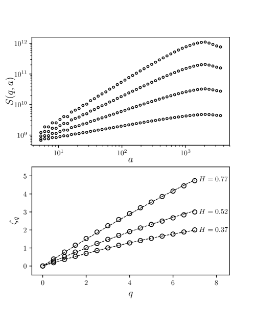
This result is illustrated in Fig. 3 where the estimated structure functions

$$S(q,a)=\sum_{k}|X(k+a)-X(k)|^{q}$$ (30)

are computed on realizations of log-normal versions of $X(t)$ with $H=0.36$, $0.51$ and $0.76$ respectively and $\lambda^{2}=0.025$. In each case, the integral scale has been set to $T=2048$ and the overall sample length corresponds to 16 integral scales. In the top panel of Fig. 3 we have plotted $\log_{10}S(q,a)$ as a function of $\log_{10}a$ in the case $H=0.36$. We see that a power-law behavior extends from the smallest scale up to the integral scale. The estimated $\zeta_{q}$ spectrum, as obtained from a linear fit of these log-log plots, are reported in the bottom panel (symbols $\circ$). In the three cases, we obtain, within a good precision, the expected scaling exponents:

$$\zeta_{q}=\left(H+\frac{\lambda^{2}}{2}\right)q-\frac{\lambda^{2}}{2}q^{2}$$ (31)

represented by the dashed lines. Let us notice that in the case $H=0.5125$, one has $\zeta_{2}=2$ and therefore the successive increments of $X(t)$ are uncorrelated as in the Brownian motion (see next Section). When $H=0.36$ (precisely $H=0.3585$), one has $\zeta_{3}=1$ as expected for the increments of the longitudinal velocity in fully developed turbulence Frisch (1995).

Figure 4: Estimated correlation function of the increments of $X(t)$ for $H=0.36$ (top panels) and $H=0.76$ (bottom panels). In both cases $\omega_{\ell}(t)$ is a Gaussian process of intermittency coefficient $\lambda^{2}=0.025$. The synthetizing wavelet $\varphi(t)$ is a ”mexican hat” wavelet, $g^{(2)}(t)$ defined in Eq. (15). As expected when $H$ is small enough increments are anti-correlated while for $H$ large enough. The expected power-law behavior (34) are represented by the solid lines in left panels.

It is well known that the spectrum of scaling exponents $\zeta_{q}$ can be, for a large class of functions, related to the singularity spectrum, i.e., the fractal (Haussdorf) dimension of the sets of iso-Hölder regularity Parisi and Frisch (1985); Jaffard (1997a, b); Barral and Mandelbrot (2004). This is the so-called multifractal formalism. At this stage, it is tempting to conjecture that the result proven by Barral and Seuret for random wavelet series Barral and Seuret (2005) is also valid in the framework introduced here and that the multifractal formalism holds for continuous wavelet cascades. In our context, the Barral-Seuret result would say that $D(h)$ the singularity spectrum of $X(t)$, can be simply obtained from $D_{M}(\alpha)$, the singularity spectrum of the underlying log-infinitely divisible cascade $dM_{t}=\lim_{\ell\to 0}e^{\omega_{\ell}(t)}dt$. More precisely, if $D_{M}(\alpha)$ is the singularity spectrum of the continuous cascade $M(t)$ as provided by the multifractal formalism Barral and Mandelbrot (2004), i.e., in the range where $1+\min_{q}(q\alpha-\phi(q))>0$, one has

$$D_{M}(\alpha)=1+\inf_{q}(q(\alpha-1)+\phi(q))$$

and thus, from definition (23),

$$D_{M}(\alpha)=F(\alpha+H-1)\;.$$ (32)

Then the analog of Barral-Seuret result (Theorem 1.1 of Barral and Seuret (2005)) result would assert that the singularity spectrum $D(h)$ of $\cal W$-cascades is provided by $D(h)=D_{M}(h+1-H)$ which according to (32), would simply mean that the singularity spectrum of $X(t)$ is $D(h)=F(h)$ in the range where $F(h)$, as given by (23) is positive. Since $F(h)=1+\inf_{q}(qh-\zeta_{q})$ is the Legendre transform of the spectrum of scaling exponents of wavelet transform structure functions, this would imply that the multifractal formalism holds for continuous $\cal W$-cascades.

IV.2 Increment correlation functions and magnitude covariance

In this section, we study the behavior of various correlation functions associated with the increments (or wavelet coefficients) or the powers of their absolute values.

Let us first define the increment correlation function

$$\rho(a,\tau)=\mathbb{C}\mathrm{ov}\left(\delta_{a}X(t),\delta_{a}X(t+\tau)\right)=\mathbb{E}\left[\delta_{a}X(t)\delta_{a}X(t+\tau)\right]$$ (33)

It is easy to show that, when $a\ll\tau$, one has Rambaldi et al. (2018)

$$\rho(\tau)\simeq\frac{\partial}{\partial\tau}\tau^{-1}\mathbb{E}\left[\delta_{\tau}X(t)^{2}\right]$$

and therefore, from Eq. (29), one has:

$$\rho(\tau)\simeq A\tau^{\zeta_{2}-2}\;.$$ (34)

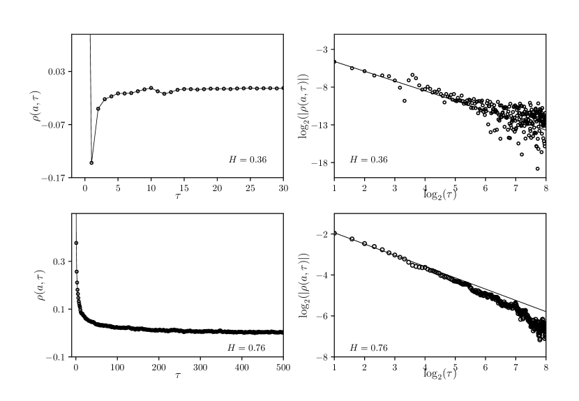
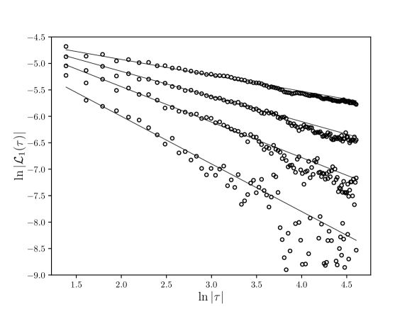
Let us remark that if $\zeta_{2}<1$, then the prefactor $A$ is negative and the increments are anti-correlated while if $\zeta_{2}>1$, the correlations are positive. This is reminiscent of the correlations of a fractional Brownian motion Mandelbrot and Ness (1968); Taqqu and Samorodnisky (1994) increments where $\zeta_{2}=2H$ and for which the value $H=1/2$ separates the regimes of negatively and positively correlated fluctuations. The behavior (34) is illustrated empirically using two samples of $X(t)$ with respectively $H=0.36$ and $H=0.76$ while $\lambda^{2}=0.025$ and $T=2048$ in both cases. The empirical increments correlation function have been estimated at scale $\tau=1$ from samples of length 16 integral scales. As expected, one can observe, in the right top and right bottom panels, a power-law behavior in both cases and that $\zeta_{2}-2$ provides a good fit (solid lines). In the left panels, we see that the process with $H=0.36$, corresponding to $\zeta_{2}=0.695$ is characterized by anti-correlated increments while the one with $H=0.76$, corresponding to $\zeta_{2}=1.495$, has positively correlated increments.

The behavior correlation function of the absolute power of the increments can be inferred from the self-similarity properties of the wavelet transform $W(x,a)$. The same kind of scaling argument as previously used to establish the scaling of structure functions can be used. Indeed, from Eq. (27), one has, for $a\leq\tau\leq T-\kappa a$:

$$\mathbb{E}\left[|W(x_{0},ra_{0})|^{q}|W(x_{0}+r\tau_{0},ra_{0})|^{p}\right]=r^{\zeta_{q+p}}\mathbb{E}\left[|W(x_{0},a_{0})|^{q}|W(x_{0}+\tau_{0},a_{0})|^{p}\right]$$ (35)

Let us now choose $\varepsilon\ll 1$ and set $T^{\prime}=\frac{T}{1+\varepsilon}$. Let us consider $ra_{0}=a$, $r\tau_{0}=\tau$ and $a=\varepsilon\tau$. The previous equation can be rewritten as:

$$\mathbb{E}\left[|W(x_{0},a)|^{q}|W(x_{0}+\tau,a)|^{p}\right]=\left(\frac{\tau}{T^{\prime}}\right)^{\zeta_{q+p}}\mathbb{E}\left[|W(x_{0},\varepsilon T^{\prime})|^{q}|W(x_{0}+T^{\prime},\varepsilon T^{\prime})|^{p}\right]$$ (36)

If one considers $\varepsilon\to 0$ (i.e. one chooses $a$ very small), then $T^{\prime}\simeq T$ and $W(x_{0},\varepsilon T^{\prime})$ becomes independent from $W(x_{0}+T^{\prime},\varepsilon T^{\prime})$ and one has:

$$\mathbb{E}\left[|W(x_{0},\varepsilon T^{\prime})|^{q}|W(x_{0}+T^{\prime},\varepsilon T^{\prime})|^{p}\right]\simeq\mathbb{E}\left[|W(x_{0},\varepsilon T^{\prime})|^{q}\right]\mathbb{E}\left[|W(x_{0}+T^{\prime},\varepsilon T^{\prime})|^{p}\right]\sim K_{p,q}(a)\left(\frac{\tau}{T}\right)^{-\zeta_{q}-\zeta_{q}}$$ (37)

where $K_{p,q}(a)$ is a constant that depends on $a$. Given the scaling (29), this entails, for a fixed small value of $a$:

$$\mathbb{E}\left[|W(x_{0},a)|^{q}|W(x_{0}+\tau,a)|^{p}\right]\sim K_{p,q}(a)\left(\frac{\tau}{T}\right)^{\zeta_{p+q}-\zeta_{q}-\zeta_{p}}$$ (38)

showing that correlation functions of the powers of the wavelet transform absolute value, behave, at a given scale, as a power-law as a function of the time lag $\tau$ with a scaling exponent $\zeta_{p+q}-\zeta_{p}-\zeta_{q}$. It is important to notice that this exponent does not depend on $H$ and is only provided by the $\phi(q)$ the non-linear part of $\zeta_{q}$.

Figure 5: Estimated correlation function of the absolute increments of $X_{LN}(t)$ for $H=0.37$ ($\circ$) and $H=0.77$ (solid lines). As expected they both behave as $\tau^{-\lambda^{2}}$ independently of $H$ (represented by the dashed line in the bottom panel).

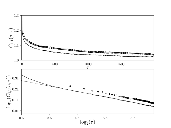
This behavior is illustrated in Fig. 5 where we have plotted the estimation of absolute increments (i.e. in the case $p=q=1$) for the two log-normal processes with $H=0.36$ and $H=0.77$ considered previously. As expected both behave, independently of $H$, as $\tau^{\zeta_{2}-2\zeta_{1}}$ that corresponds, according to Eq. (31) to the power-law $\tau^{-\lambda^{2}}$ (represented by the dashed line in the bottom panel).

Eq. (38) can be used to compute the behavior of magnitude covariance as defined in Arneodo et al. (1998a); Muzy et al. (2000). Indeed, since:

$$\mathbb{C}\mathrm{ov}\left(\ln|W(x_{0},a)|,\ln|W(x_{0}+\tau,a)|\right)=\frac{\partial_{q}\partial_{p}\ln\mathbb{E}\left[|W(x_{0},a)|^{q}|W(x_{0}+\tau,a)|^{p}\right]}{\partial p\partial q}\bigg{\rvert}_{q,p=0}\;,$$ (39)

we obtain the well known logarithmic magnitude covariance for multifractal processes Arneodo et al. (1998a); Muzy et al. (2000):

$$\mathbb{C}\mathrm{ov}\left(\ln|W(x_{0},a)|,\ln|W(x_{0}+\tau,a)|\right)\simeq\zeta^{\prime\prime}(0)\ln\left(\frac{\tau}{T}\right)=-\lambda^{2}\ln\left(\frac{\tau}{T}\right)$$ (40)

where we defined the intermittency coefficient as $\lambda^{2}=-\zeta^{\prime\prime}(0)$.

V Skewness and leverage effect: applications to turbulence and stock market data

V.1 Skewness of increment pdf at all scales

Because of the self-similarity relationship (27), one can also expects a scaling of odd moments of the wavelet transform, i.e., $\forall k\in\mathbb{N}$, $\forall a\leq T$,

$$S^{\star}(2k+1,a)=\mathbb{E}\left[W(x,a)^{2k+1}\right]=V_{2k+1}\;a^{\zeta_{2k+1}}$$ (41)

This shows in particular that generically, the skewness

$$\frac{\mathbb{E}\left[W(x,a)^{3}\right]}{\mathbb{E}\left[W(x,a)^{2}\right]^{3/2}}\sim a^{\zeta_{3}-\frac{3}{2}\zeta_{2}}$$

increases (in absolute value) when $a\to 0$. The computation of the constant $V_{2k+1}$ for a given waveform $\varphi$ is tedious and can be only written as an intricate multiple integral but it can be shown it is non-zero unless $\varphi$ satisfies very specific conditions (see Fig. 7). This shows that our approach, unlike constructions bases on classical random measures, generically leads to skewed multifractal processes with a skewness that, like the flatness, increases as one goes from coarse to fine scales.

Figure 6: Estimated “standardized” probability density function (pdf) of the “wavelet coefficients” at scale $a$, $p_{a}(w)$. At each scale, $a=T$,$T\over 8$,$T\over 64$,$T\over 512$, $T\over 4096$, where $T$ stands for the integral scale, we have displayed $\ln p_{a}(w)$ up to an additive constant for the sake of clarity: pdf at small scales are displayed above pdf at coarser scales. On the top left and right panels the considered $\cal W$-cascade $X(t)$ is a log-normal process with a synthetizing wavelet $\varphi$ that is a odd function ($g^{(1)}(t)$, the first derivative of the Gaussian function). We can check that, due to the intermittency, the flatness increases from large to small scales. On the left panel the analyzing wavelet is odd since it is $\psi(t)=\delta^{(1)}(t)$ (the one that corresponds to the increments of $X(t)$) while on the right panel one uses $\psi(t)=\delta^{(2)}(t)$ and thus considers the second order increments. As expected, one clearly observes, like in turbulence, skewed distributions of increments at all scales. The second order increments are distributed with a symmetric law. On the bottom panels, the opposite effect is observed since the process $X(t)$ as been constructed using a symmetric wavelet, namely $g^{(2)}(t)$, the second order derivative of the Gaussian function.

Figure 7: Signed third order structure function $S^{\ast}(3,a)$ as a function of the scale $a$. On the left panel the mean order 3 moment of the increments is computed on $X(t)$ corresponding to the anti-symmetric synthetizing wavelet $g^{(1)}(t)$ (Eq. (15)). This confirms the (negative) skewness already illustrated in Fig. 6 and that, as expected for turbulence, $S^{\ast}(3,a)$ behaves as a linear function. In the right panel, $X(t)$ is built using the non-symmetric wavelet depicted in Fig. 1. The third order structure function function behaves as a linear function and skewness can be observed for both first ($\circ$) and second order increments (solid line).

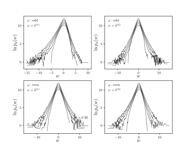
The scaling relationship (41) indicates that the skewness will be zero at all scales if it vanishes at the largest scale $T$. It is noteworthy that this may be the case if the synthetizing wavelet $\varphi$ in Eq. (9) is an even or odd function. Indeed, if the wavelet $\varphi(t)$ is a symmetric function, because $\omega_{\ell}(t)\stackrel{{\scriptstyle{\cal L}}}{{=}}\omega_{\ell}(-t)$, we see from definition (9) that $X_{\ell}(t)$ is invariant by time reversal, i.e., one has $X_{\ell}(-t)\stackrel{{\scriptstyle{\cal L}}}{{=}}X_{\ell}(t)$. It thus results that if the analyzing wavelet an odd function (as e.g. for the increments $\delta_{\tau}X(t)$) the wavelet transform of $X(t)$ will have a symmetric law implying that all odd moments are zero. In order to observe some skewness in the increment law, it is thus necessary to consider non-symmetric synthetizing wavelets $\varphi$. Along the same line, if the synthetizing wavelet $\varphi(t)$ is anti-symmetric, then $X(t)$ is odd by time reversal, i.e., $X_{\ell}(-t)\stackrel{{\scriptstyle{\cal L}}}{{=}}-X_{\ell}(t)$ and if the analyzing wavelet is even (as e.g. when one computes the second order increments of $X(t)$, $\delta^{(2)}_{\tau}X(t)=X(t+2\tau)+X(t)-2X(\tau)$), the wavelet transform will have a symmetric law. This means that if a skewness is observed in both first and second order increments, the wavelet $\varphi(t)$ is neither an even nor an odd function.

Figure 8: Paths of turbulence velocity field and stock market data as compared to their $\cal CW$-cascade models. In the top left panel are represented the longitudinal velocity field space variations (in $m/s$) obtained in a high Reynolds number turbulence experiment ($R_{\lambda}\simeq 700$) realized by Castaing et al. Castaing et al. (1994). The top right panel corresponds to the cascade model obtained by fitting the turbulence multiscaling but also the skewness of law of first order increments. In the left bottom panel is plotted the detrended daily variations of the logarithm of the Dow-Jones index over the more than 4 decades (from 1939 to 1985). The right bottom panel represents its $\cal CW$-cascade model where we mainly account for the skewness of second order increments. We can see that the ”ramp” like behavior of turbulence data and ”arch” like patterns of stock market data are remarkably well reproduced by ${\cal CW}$-cascades.

These behaviors are illustrated in Fig. 6 where whe have displayed the probability density functions (pdf) of the first and second increments at different scales of two versions of log-normal continuous wavelet cascades $X(t)$ that are respectively antisymmetric and symmetric by time reversal. In the first case, we used $\varphi=g^{(1)}$ while in the second case $\varphi=g^{(2)}$ (see Eq. (15)). In both cases, we chose $\omega_{\ell}$ as a log-normal cascade with $\lambda^{2}=0.025$, an integral scale $T=2^{12}$ and $H=0.355$. In that respect, according to (31), $\zeta_{3}=1$ and $X(t)$ was designed to mimic the main features of velocity records in experiments of fully developed turbulence. All the estimations have been performed on a sample of length $128$ integral scales. All the probability density functions reported in Fig. 6 are standardized, i.e., represent the distribution of increments normalized by their root-mean-square. The are displayed in semi-log scales and shifted so that large scale distribution are below fine scale ones. In that way, one can clearly observe the intermittency as an increasing of the flatness from large to small scales. We can check in the top-right (resp. bottom-left) panel of Fig. 6 that if $\varphi$ is odd (resp. even), the second (resp. first) order increments are symmetrically distributed. We can see the in top-left panel that, at all scales the increments of the anti-symmetric version of $X(t)$ are negatively skewed. The shapes of these skewed pdf, with an increasing flatness are strikingly similar to distribution of longitudinal velocity increments in fully developed turbulence Castaing et al. (1990, 1994). In the symmetric version of $X(t)$, the skewness is only observed on its second order increments (bottom-right panel).

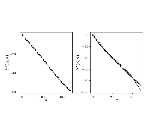
The fact that an anti-symmetric synthezing wavelet allows one to reproduce the observed skewness behavior of the velocity field in turbulence is directly illustrated in left panel of Fig. 7: we have plotted, in linear scale, the signed third order structure function $S^{\star}(3,a)$ as a function of the scale $a$ estimated for a log-normal $\cal CW$-cascade calibrated precisely to model the spatial fluctuations of the longitudinal velocity in turbulence (i.e., one sets $\zeta_{3}=1$ and $\lambda^{2}=0.025$). It can be checked that for such a process we have $S^{\star}(3,a)=-Ka$. In full analogy with turbulence, one can wonder if $K$ could not be chosen such that, as in Kolmogorov theory, $K=\frac{4}{5}\varepsilon$ where $\varepsilon$ is the mean dissipation rate $\varepsilon\sim\mathbb{E}\left[a^{-1}\nu\int_{0}^{a}dt(\frac{\partial}{\partial t}X(t))^{2}\right]\;$ Frisch (1995). Since $X(t)$ is not differentiable, in order for this to be meaningful, we show, in Appendix E, that the so-called “dissipative anomaly” Eyink and Sreenivasan (2006) property of the velocity field can be reproduced within our framework: if one chooses a “viscosity” $\nu(\ell)$ such that $\nu(\ell)\sim\ell^{4/3-\lambda^{2}}$, then:

$$\lim_{\ell\to 0}\nu(\ell)\;\mathbb{E}\left[\left(\frac{\partial X_{\ell}(t)}{\partial t}\right)^{2} \right]=\varepsilon\;,$$ (42)

for some $0<\epsilon<\infty$. Let us point out that it is likely that, from the definition Eq. (9), one could establish the following generalization of Eq. (42):

$$\nu(\ell)\left(\frac{\partial X_{\ell}}{\partial t}\right)^{2}dt\underset{\ell\rightarrow 0}{\longrightarrow}\varepsilon(dt)$$

where $\varepsilon(dt)$ represents a singular measure corresponding to the multifractal dissipation men in the limit of vanishing viscosity and the convergence being interpreted in a weak sense.

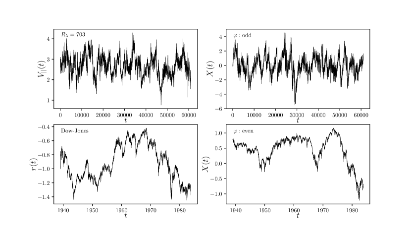
Since the (negative) skewness of turbulence fields appears mainly on first order increments (or on odd analyzing wavelets), as one can see in the top panels of Fig. 8, it can be directly visualized as “ramp” like (i.e. a slow increase followed by a rapid fall) patterns on the velocity profile and its model. This behavior is very different from the ”arch” like shapes that can be associated with the negative skewness of the second order increments. Such a feature is obviously present in the fluctuations of market prices as illustrated in the example of the Dow-Jones index the bottom left panel of Fig. 8. In the right panels, we plotted sample paths of the corresponding log-normal models for turbulence ($H=0.355$, $\lambda^{2}=0.025$ and $\varphi=g^{(1)}$) and stock market data ($H=0.51$, $\lambda^{2}=0.025$ and $\varphi=g^{(2)}$).

A close inspection of the Dow-Jones evolution in the bottom-left panel of Fig. 8 reveals that this process has not only skewed second order increments by also display skewed first order increments. Indeed, it is well known that financial return variations are characterized by rapid large drops that are followed by slower upward moves. It thus results that, in order to model the dynamics of market prices, a $\cal CW$-cascade should involve a wavelet that is neither odd nor even. In the left panel of Fig. 7, we have computed the behavior of $S^{\star}(3,a)$ as a function of $a$ for both first and second order increments when the wavelet is the non-symmetric wavelet displayed in Fig. 1(c) (the other parameters are those chosen for turbulence). We see that both types of increments are characterized by a skewness of comparable magnitude since one observes third order moments a behaves as similar linear functions of the scale. As discussed below, asymmetric synthetizing wavelets allow one to account for another feature observed on stock market data, namely the leverage effect.

V.2 Leverage effect

The fact that the sythetizing wavelet $\varphi(t)$ has no particular symmetry can be reflected by different statistical quantities. As discussed notably by Pommeau Pomeau, Y. (1982), there exists a wide variety of correlation functions that allow one to reveal the lack of time reversal symmetry of a process $X(t)$. The “leverage” function is a particular example of such a measure. It consists in computing the correlation between the increments at some scale and their ”amplitude” (e.g. their absolute value and their squared value) after or before some time lag $\tau$ Bouchaud et al. (2001); Pochart and Bouchaud (2002); Bacry et al. (2012):

$${\cal L}_{q}(\tau)=Z_{q,\ell}^{-1}\mathbb{E}\left[\delta_{\ell}X(t)|\delta_{\ell}X(t+\tau)|^{q}\right]$$ (43)

where $Z_{q,\ell}^{-1}$ is a properly chosen normalization constant: for example, in Bouchaud et al. (2001), the authors studied ${\cal L}_{2}$ with $Z_{2,\ell}=\mathbb{E}\left[\delta X_{\ell}^{2}\right]^{2}$. In general one will consider the behavior in the small scale regime, i.e., the limit $\ell\to 0$ with a wel chosen normalization. The so-called “leverage effect” is a property that has been empirically observed on stock prices and stock market indices indicating that past returns are (negatively) correlated with future volatility (i.e. ${\cal L}_{q}(\tau)<0$ for $\tau\geq 0$) while the reverse is not true (${\cal L}_{q}(\tau)\simeq 0$ for $\tau<0$). In that context ”returns” means increments of log-price while ”volatility” stands for squared or absolute returns. The leverage effect can be intuitively explained by the fact that, after a large price drop, some kind of panic takes place with a large uncertainty and thus a large volatility results. The symmetric situation, i.e a large upward price move, does not induce any crisis and therefore does not trigger any noticeable volatility variation.

Figure 9: Scaling of the leverage function. Estimated curves $|{\cal L}_{1}(\tau)|$ are plotted as a function of $|\tau|$ is double logarithmic scale (symbols ($\circ$)). The estimations have been performed on samples of lenght $L=2^{17}$ of log-normal ${\cal CW}$-cascades with $\lambda^{2}=0.025$, $T=2^{10}$ and, from top to bottom, $H=0.7,0.51,0.33$ and $0.1$. The solid lines represent the corresponding theoretical power-laws of exponent $H-1-\phi(2)$.

Figure 10: Leverage functions ${\cal L}_{1}(\tau)$ estimated for a log-normal $\cal{CW}$-cascade with $H=0.515$ and $\lambda^{2}=0.025$ (solid lines). The various curves correspond to different asymmetry factors $\alpha$ in the synthetizing wavelet defined in Eq. (45), namely $\alpha=\frac{1}{8}$, $\frac{1}{3}$, $\frac{1}{2}$ and $1$. One sees that the behavior at lags $\tau>0$ does not depend on $\alpha$ whereas the leverage function at negative lags becomes smaller and smaller as the asymmetry increases. For comparison purpose, the estimated leverage function from daily Dow-Jones index data are also reported (grey curve).

Different attempts to account for this effect within the standard class of econometric models have been proposed Bouchaud et al. (2001); Perello and Masoliver (2003). Since the class of Multifractal Random Walk as described in Sec. II.1 remarkably accounts for many of “stylized facts” of asset fluctuations, some authors considered different variants of these models that break the time reversal symmetry by introducing specific correlations between cascade and noise terms Pochart and Bouchaud (2002); Bacry et al. (2012). But as mentionned in the introductory section, such approaches cannot lead to well defined continuous time limits unless the noise has long-range correlations Pochart (2003); Bacry et al. (2012); Chevillard et al. (2017b). Since continuous $\cal W$-cascades are generically not invariant by time reversal one expects that it should be possible to account for the leverage effect by a specific choice of the synthetizing wavelet $\varphi$. According to the definitions (43) and (9), ${\cal L}_{q}(\tau)$ can be expressed as an intricate integral. In Appendix F, we show, using some heuristic approximations, that, when $q=1$, the leverage function behaves as:

$${\cal L}_{1}(\tau) \underset{\tau\gg\ell}{\sim} C_{+}|\tau|^{H-1-\phi(2)}$$

$${\cal L}_{1}(\tau) \underset{\tau\ll-\ell}{\sim} C_{-}|\tau|^{H-1-\phi(2)}$$

where both scaling laws are valid in the range $|\tau|\ll T$. We have shown that the prefactors $C_{+}$ and $C_{-}$ depend on the synthetizing wavelet $\varphi$ as:

$$C_{+} = -\int_{0}^{+\infty}\!\!s^{H-1}ds\int\!du\varphi\left(u\right)C_{s}^{\prime}(su+1)$$

$$C_{-} = -\int_{0}^{+\infty}\!\!s^{H-1}ds\int\!du\varphi\left(u\right)C_{s}^{\prime}(su-1)$$

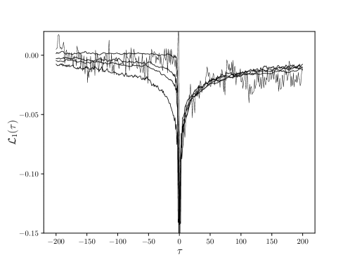
with $C_{s}(z)=\mathbb{E}\left[e^{\omega_{s}(t)+\omega_{s}(t+z)}\right]$. This scaling law is illustrated in Fig. 9 where we have checked, using estimations from simulated data, it holds for different values of $H$ in the case of a log-normal cascade built with an anti-symmetric wavelet. Notice that from the previous expression, $C_{-}$ and $C_{+}$ are not necessarily equal and the leverage effect could therefore be observed when the leverage ratio:

$$\kappa=\frac{C_{+}}{C_{-}}$$ (44)

is very large (i.e. $\kappa\gg 1$).

Figure 11: Evolution of the leverage ratio $\kappa$ (Eq. (44)) as a function of the coefficient $\alpha$ characterizing the asymmetry of the synthezing wavelets defined in (45). The numerical integrations have been performed in the log-normal case with $\lambda^{2}=0.025$ and $H=1/2+\lambda^{2}$. The symbols ($\circ$) represent the value of $\kappa$ as estimated from the empirical leverage function obtained from simulated data of length 128 $T$ with $T=2^{13}$.

For illustration purpose and in order to handle reasonable expressions, let us consider the “simple” case when $\varphi(t)$ is a piece-wise constant function:

$$\varphi(t)=\alpha^{-1}\mathbb{I}_{[0,\alpha)}(t)-\mathbb{I}_{[-1,0)}(t)$$ (45)

where $0<\alpha<1$ controls the wavelet asymmetry.

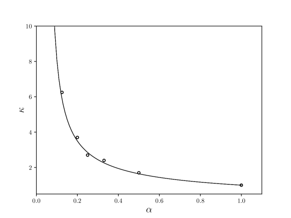
In Fig. 10 we have plotted the leverage function estimated from numerical simulations of log-normal ${\cal CW}$-cascades with a synthezing wavelet corresponding to Eq. (45) with different asymmetry factors $\alpha=1/8,1/3,1/2$ and $1$. We chose $T=2^{13}$, $\lambda^{2}=0.025$ and $H=0.51$ so that the increments are uncorrelated ($\zeta_{2}=1$). We first clearly see that the behavior for positive lags appears to not depend on $\alpha$ while the situation is very different for negative lags: as $\alpha$ decreases one sees that the leverage function lessens more and more. One goes from a symmetric leverage function in the case $\alpha=1$ to a situation where it is almost zero at negative lags. This latter case is very interesting to reproduce the empirical features observed on stock market: for comparion we have plotted the leverage function estimated from the Dow-Jones index daily returns over a period extending from 1939 to 2018 (grey line in Fig. 10). These empirical findings show that the leverage ratio strongly depends $\alpha$ and becomes arbitrary large when $\alpha$ is small. Even if it is possible to show that the constants $C_{\pm}$ are bounded in the case when $\varphi$ is defined by Eq. (45), their exact value can however be hardly obtained or approximated under a closed form. We then estimated them by means of a numerical integration. The so computed leverage ratios are reported in Fig. 11. In the case when $\alpha=1$, we naturally recover the fact that the leverage effect is not present while we observe that $\kappa$ strongly increases for small $\alpha$. Notice that our numerical estimations confirm that both $C_{+}$ and $C_{-}$ are negative in the range $0.1\leq\alpha\leq 1$. We also observed that $C_{+}$ is almost independent of $\alpha$ while $C_{-}$ becomes arbitrary small as $\alpha\to 0.048$ where it changes its sign. It thus seems possible, within this model, to obtain a ”perfect” leverage effect with an infinite leverage ratio corresponding to a vanishing leverage function in the domain $\tau<0$. These numerical computations of the leverage ratio have been checked using empirical estimation from numerical simulations (symbols $\circ$).

VI Summary and prospects

In this paper we have proposed a new way to build random multifractal functions with stationary increments, exact scaling and self-similarity properties. Our model just consists in extending former $\cal W$-cascades by replacing the framework of orthogonal wavelet basis by that of continuous wavelet transform and the discrete multiplicative weights by their log-infinitely divisible counterpart, i.e. the process $e^{\omega_{\ell}(t)}$ involved in the construction of continuous cascade measures. We have shown that our construction provides almost surely Liphscitz regular paths and studied its self-similarity and scaling properties. As emphasized in Sec.V, $\cal CW$-cascades are in general skewed multifractal processes and are characterized by a non-symmetric correlation between increment signs and amplitudes (the so-called ”leverage effect”). As far as applications to turbulence are concerned, since our framework can easily reproduce the skewed intermittency phenomenon observed for the velocity fluctuations, together with the dissipative anomaly, it provides undoubtedly a promising way to account for many stochastic aspects of fluid dynamics in regimes of fully developed turbulence. It that respect, vector and 3-dimensional extensions of $\cal CW$-cascades with the possibility of introducing well known dynamical properties like incompressibility (as e.g. in Chevillard et al. (2010); Pereira et al. (2016)) could be interesting in order to get a more realistic model.

Beyond applications to specific contexts and the previously mentioned problems, a fundamental question is to know which features of the sythetizing wavelet remain observable through the associated continuous cascade. Is there a analog of the famous black holes ”no-hair theorem” Misner et al. (1973) in the present framework ? This ”inverse problem” is interesting since we already known that some important properties like skewness, the behavior of the leverage function, the prefactor values in scaling relationships may depend on the specific wavelet shape but the issue is to precisely know in what respect and also which properties of $\varphi$ (like e.g. the number of vanishing moments, the moment values,…) can be recovered from empirical data.

Finally, let us mention that, by simply replacing $e^{\omega_{\ell}(t)}$ by its lacunary version introduced in Muzy and Baïle (2016), our framework may also allow one to build random functions that are almost everywhere smooth and singulular on random Cantor sets. One could also slightly extend the definition of ${\cal CW}$-cascades in order to build a stationary variant of the class of lacunary wavelet series that possess oscillating singularities defined and studied by Arneodo et al. Arneodo et al. (1997a, 1998c). Such processes are not self-similar but possess a self-similar wavelet transform. All these prospects will be considered in a future research.

Appendix A Continuous cascade construction

The process $\omega_{\ell}(x_{0})$ in the definition (2) is constructed as follows: On considers the time scale half-plane $(t,s)\in\mathbb{R}\times\mathbb{R^{+\ast}}$ and the natural measure $dm(t,s)=s^{-2}dtds$ which gives the area of any set ${\cal S}$ as:

$$|{\cal S}|=\int_{\cal S}dm(t,s)=\int_{\cal S}s^{-2}dtds\;.$$

Within this framework, one considers $dP(t,s)$ a random infinitely divisible ”white noise” (the so-called ”independently scattered random measure”) such that, the measure of a given set ${\cal S}$, $P({\cal S})=\int_{\cal S}dP(t,s)$ is an infinitely divisible random variable of characteristic function:

$$\mathbb{E}\left[e^{ikP({\cal S})}\right]=e^{|{\cal S}|\phi(ik)}$$ (46)

where $\phi(q)$ is the cumulant generating function associated with an infinitely divisible law as provided by the celebrated Levy-Khintchine Theorem Feller (1971). For example, if $\phi(q)=qH-\lambda^{2}q^{2}/2$, $dP(t,s)$ is simply a Gaussian white noise of mean $Hs^{-2}dtds$ and variance $\lambda^{2}s^{-2}dtds$.

Let us now, as in Muzy and Bacry (2002); Bacry and Muzy (2003), consider $dP(t,s)$ such that $\phi(1)=0$ and define, for any $T>0$, the cone like domain ${\mathcal{A}}_{a}(x_{0})$ as:

$$(x,s)\in{\mathcal{A}}_{a}(x_{0})\Leftrightarrow\left\{s\geq a,\;2|x-x_{0}|\leq\min(s,T)\right\}$$ (47)

Figure 12: The domains ${\mathcal{A}}_{a}(x_{0})$ and ${\mathcal{A}}_{a}(x_{1})$ and their intersection.

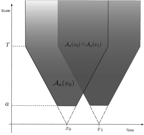
The shape of ${\mathcal{A}}_{a}(x_{0})$ is depicted in Fig. 12. The process $\omega_{\ell}(x)$ is then simply defined as:

$$\omega_{\ell}(x)=P\left[{\mathcal{A}}_{\ell}(x)\right]\;.$$ (48)

Let $\rho_{\ell}(\tau)$ be the area of the set ${\mathcal{A}}_{\ell}(x_{0})\cap{\mathcal{A}}_{\ell}(x_{0}+\tau)$ (see Fig. 12). A direct computation leads to:

$$\rho_{\ell}(\tau)=\left\{\begin{array}[]{ll}\ln\left(\frac{T}{\ell}\right)+1-\frac{\tau}{\ell}&\mbox{if}~{}\tau\leq\ell\;,\\ \ln\left(\frac{T}{\tau}\right)&\mbox{if}~{}T\geq\tau\geq\ell\;,\\ 0&\mbox{if}~{}\tau>T\;.\end{array}\right.$$ (49)

In Bacry and Muzy (2003) it is shown that the characteristic function of $\omega_{\ell}(x)$, for any $q\in\mathbb{N}^{*}$, $(x_{1},x_{2},\ldots,x_{q})\in\mathbb{R}^{q}$ with $x_{1}\leq x_{2}\leq\ldots\leq x_{n}$ and $(p_{1},p_{2},\ldots,p_{q})\in\mathbb{R}^{q}$ is given by:

$$\mathbb{E}\left[e^{\sum_{m=1}^{q}ip_{m}\omega_{\ell}(x_{m})}\right]=e^{\sum_{j=1}^{q}\sum_{k=1}^{j}\alpha(j,k)\rho_{\ell}(x_{k}-x_{j})}$$ (50)

whare $\alpha(j,k)$ are coefficients defined in Bacry and Muzy (2003) that satisfy:

$$\sum_{j=1}^{q}\sum_{k=1}^{j}\alpha(j,k)=\phi\left(\sum_{k=1}^{q}p_{k}\right)\;.$$ (51)

Expression (50) entails in particular that $\rho_{\ell}(\tau)$ corresponds to the covariance (when it exists) of $\omega_{\ell}(x)$ and $\omega_{\ell}(x+\tau)$. Notably, in the case when $dP(t,s)$ is a Gaussian white noise, the above construction of $e^{\omega_{\ell}(t)}$ is an example of the celebrated Kahane Multiplicative Chaos measure Kahane (1985); Rhodes and Vargas (2014) and corresponds to the measure originally proposed in the MRW construction Muzy et al. (2000); Bacry et al. (2001).

Appendix B Weak convergence of $X_{2^{-n}}(t)$ in the space of continuous functions.

Let us show that the series

$$X^{(n)}(t)=X_{2^{-n}}(t)=\int_{2^{-n}}^{T}\!s^{H-2}ds\!\int_{-\infty}^{+\infty}\!\!\!e^{\omega_{s}(b)}\varphi\left(\frac{t-b}{s}\right)db$$ (52)

converges in the weak sense when $n\to\infty$ in the space of continuous functions.

We first need a result that can be found e.g. in Muzy and Baïle (2016) that can be directly deduced from the definition of $\omega_{s}(t)$ in Section A: for all $s^{\prime}\leq s\leq T$, one has:

$$\mathbb{E}\left[e^{\omega_{s}(u)+\omega_{s^{\prime}}(v)}\right]=e^{(\phi(2)-2\phi(1))\rho_{s}(u-v)+\phi(1)(\rho_{s}(0)+\rho_{s^{\prime}}(0))}$$

where $\rho_{s}(\tau)$ is defined in Eq. (49). From this expression, one deduces:

$$\mathbb{E}\left[e^{\omega_{s}(u)+\omega_{s^{\prime}}(v)}\right]\leq C_{1}s^{\phi(1)-\phi(2)}s^{\prime-\phi(1)}$$

i.e., assuming (10),

$$\mathbb{E}\left[e^{\omega_{s}(u)+\omega_{s}^{\prime}(v)}\right]\leq C_{1}s^{-\phi(2)}$$ (53)

Let us first show that all finite dimensional distributions of $X^{(n)}$ converge. For that purpose it suffices to show that for all $m,n\to 0$

$$\mathbb{E}\left[\left(X^{(n)}(t)-X^{(m)}(t)\right)^{2}\right]\to 0$$

and therefore, assuming $n\leq m$:

$$\mathbb{E}\left[\left(\int_{2^{-m}}^{2^{-n}}\!s^{H-2}ds\!\int_{-\infty}^{+\infty}e^{\omega_{s}(b)}\varphi\left(\frac{t-b}{s}\right)db\right)^{2}\right]\to 0\;.$$

By permuting expectation and integration, we have to show that

$$\iint_{[2^{-m},2^{-n}]}ds_{1}ds_{2}(s_{1}s_{2})^{H-2}\iint db_{1}db_{2}\varphi\left(\frac{t-b_{1}}{s_{1}}\right)\varphi\left(\frac{t-b_{2}}{s_{2}}\right)\mathbb{E}\left[e^{\omega_{s_{1}}(b_{1})+\omega_{s_{2}}(b_{2})}\right]\to 0$$

Since $\varphi$ is bounded and supported by $[-1/2,1/2]$, the previous expression can be bounded by :

$$2C_{2}\int_{2^{-m}}^{2^{-n}}ds_{1}\int_{s_{1}}^{2^{-n}}ds_{2}\;(s_{1}s_{2})^{H-2}\int_{-s_{1}/2}^{s_{1}/2}\int_{-s_{2}/2}^{s_{2}/2}db_{1}db_{2}\mathbb{E}\left[e^{\omega_{s_{1}}(b_{1})+\omega_{s_{2}}(b_{2})}\right]$$

and thus, thanks to (53)

$$\mathbb{E}\left[\left(X^{(n)}(t)-X^{(m)}(t)\right)^{2}\right]\leq C_{3}2^{-n(2H-\phi(2))}\ .$$

$X^{(n)}(t)$ is therefore a Cauchy sequence provided

$$\phi(2)<2H\;.$$ (54)

In order to prove the weak convergence, it remains to establish the tightness of the sequence Billingsley (1968). Since the sequence $X^{(n)}(t)$ are continuous processes, from Swanson (2007), it suffices to show that

$$\sup_{n}\mathbb{E}\left[|X^{(n)}(t)|^{\nu}\right]<\infty\;\mbox{and}\;\sup_{n}\mathbb{E}\left[|X^{(n)}(t)-X^{(n)}(u)|^{\beta}\right]\leq C|t-u|^{\gamma}$$

for some positive $\nu,\beta$ and $\gamma$. Let us show that both assertions hold for $\nu=\beta=2$ if one supposes that (54) is satisfied. In that case, by the same kind of computation as previously, thanks to inequality (53), one can show that $\mathbb{E}\left[|X^{(n)}(t)|^{2}\right]\leq C$ where $C$ does not depend on $n$. Moreover, we have:

$$\mathbb{E}\left[(X^{(n)}(t)-X^{(n)}(u))^{2}\right] = \int_{2^{-n}}^{T}ds_{1}\int_{s_{1}}^{T}ds_{2}(s_{1}s_{2})^{H-2}\iint db_{1}db_{2}\;\mathbb{E}\left[e^{\omega_{s_{1}}(b_{1})+\omega_{s_{2}}(b_{2})}\right]$$

$$\left(\varphi\left(\frac{t-b_{1}}{s_{1}}\right)-\varphi\left(\frac{u-b_{1}}{s_{1}}\right)\right)\left(\varphi\left(\frac{t-b_{2}}{s_{2}}\right)-\varphi\left(\frac{u-b_{2}}{s_{2}}\right)\right)$$

Let us choose $\gamma$ such that

$$0<2\gamma<2H-\phi(2)\;.$$ (55)

Then the last expression can be bounded provided $\varphi(t)$ belongs to the uniform Hölder space $C^{\gamma}(\mathbb{R})$, i.e., $\exists K_{\gamma}<\infty$ such that, $\forall t,u$, $|\varphi(t)-\varphi(u)|\leq K_{\gamma}|t-u|^{\gamma}$. We thus have, using Eq. (53) and condition (55):

$$\mathbb{E}\left[(X^{(n)}(t)-X^{(n)}(u))^{2}\right]\leq K^{\prime}|t-u|^{2\gamma}$$

where

$$K^{\prime}=K_{\gamma}\int_{0}^{T}ds_{1}\int_{s_{1}}^{T}ds_{2}s_{1}^{H-1-\gamma}s_{2}^{H-1-\phi(2)-\gamma}=K_{\gamma}\frac{T^{2H-2\gamma-\phi(2)}}{(H-\gamma)(2H-2\gamma-\phi(2))}$$

does not depend on $n$. This ends the proof of the tightness of the sequence and thus establishes the weak convergence of the sequence $X^{(n)}$ towards a continuous process $X(t)$.

Appendix C Almost sure pathwise global regularity of $X(t)$

Let us consider $h_{\min}>0$ as defined in Eq. (63). We then show that, for any $L>0$, $X(t)$ has a uniform Lipschitz regularity $\alpha$ for all $\alpha<h_{\min}$ on $[0,L]$. For that purpose, we adapt the proof of Ref. Arneodo et al. (1998b) originally proposed for discrete ${\cal W}$-cascades on orthogonal wavelet basis. Let $\psi_{j,k}(t)=2^{j}\psi(2^{j}t-k)$ be a basis of $L^{2}([0,L])$ of compactly supported wavelets. For the sake of simplicity, we will not care about boundary wavelets and we will only consider wavelets $\psi_{j,k}$ that constitute a basis of $L^{2}(\mathbb{R})$ which support $S_{j,k}$ is such that $S_{j,k}\cap[0,L]\neq\emptyset$ (see e.g Mallat (1999) for details about wavelet bases on an interval). We refer to $L_{j}$ the set of indices $k$ that satisfy this property. We can, without loss of generality, assume that $|S_{j,k}|=2^{-j}$. Let $c_{j,k}$ be the wavelet coefficients $X(t)$:

$$c_{j,k}=\int\psi_{j,k}(t)X(t)dt\;.$$ (56)

From expression (18), since the kernel $K$ is bounded, $c_{j,k}$ can be controlled as:

$$|c_{j,k}|\leq K2^{-jH}\sup_{t,s\in D(j,k)}e^{\omega_{s}(t)}$$ (57)

where $D(j,k)$ stands for the domain in the time-scale plane $s\in[\kappa 2^{-j},2^{-j}]$, $t\in[2^{-j}k-\frac{s}{2},2^{-j}k+\frac{s}{2}]$ (these domains are depicted as shaded regions in Fig. 13).

In order control the regularity of $X(t)$, one can use a standard result in wavelet analysis: $X(t)$ is uniformly Lipschitz $\alpha<1$ over $[0,L]$ if and only if there exists an uniform constant $C$ and some integer $0\leq J<\infty$: that,

$$|c_{j,k}|\leq C2^{-j\alpha}\;,\;\forall j\geq J,k\in L_{j}\;.$$ (58)

Let $D_{j}$ be the time-scale set $D_{j}$ is defined as (see Fig. 13):

$$D_{j}=\bigcup_{k\in L_{j}}D(j,k)$$ (59)

and define

$$m_{j}=\sup_{(t,s)\in D_{j}}2^{-jH}e^{\omega_{s}(t)}$$ (60)

From (57) and (58), we thus have to control the probability that $m_{j}>2^{-j\alpha}$ in order to establish global Lipschitz regularity $\alpha$ of $X(t)$.

Figure 13: The domains $L_{j}$ involved in the proof of $L^{2}$ convergence. Each shaded domain represents a set $D(j,k)$ while $L_{j}$ is the set of indices $k$ for the $D(j,k)$ that cover the interval $[0,L]$.

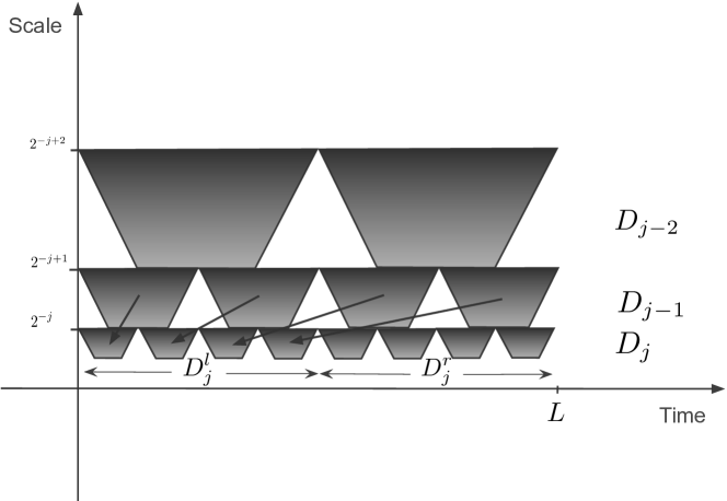
Let us suppose that $L=2^{M}<T$ where $T$ is the integral scale of $\omega_{s}(t)$, a proof for an arbitrary value of $L$ can be easily adapted by splitting the interval in small pieces of size smaller than $T$. Let us now consider that $D_{j}=D_{j}^{l}\cup D_{j}^{r}$ where $D_{j}^{l}$ and $D_{j}^{r}$ are the union of the $D(j,k)$ for the $2^{M-1}$ values of $k$ corresponding to respectively the first and the second half-part of $L_{j}$ (see Fig 13). Let $m_{j}^{l}=\sup_{(t,s)\in D_{j}^{l}}2^{-jH}e^{\omega_{s}(t)}$ and $m_{j}^{r}=\sup_{(t,s)\in D_{j}^{r}}2^{-jH}e^{\omega_{s}(t)}$. We have obviously $m_{j}=\max(m_{j}^{l},m_{j}^{r})$. By stationarity of the process $\omega_{s}(t)$, $m_{j}^{r}$ and $m_{j}^{l}$ have the same law. Moreover, from the construction of $\omega_{s}(t)$ as the integral of an infinitely divisible noise over a cone domain, they both can we written as $X^{l}Y$ and $X^{r}Y$ where $X^{r}$ and $X^{l}$ have the same law, and $X^{l},X^{r}$ and $Y$ are independent. As shown in Arneodo et al. (1998b), it results that:

$$\mathbb{P}\left[m_{j}\leq z\right]\geq\mathbb{P}\left[m_{j}^{l}\leq z\right]^{2}$$ (61)

Let us notice that one can map the domain $D_{j-1}$ used to define $m_{j-1}$ to the domains $D_{j}^{l}$ by simply considering the time-scale dilation $s\to s/2$ and $x\to x/2$. Such a mapping is illustrated by the arrows in Fig. 13. Thus, from the self-similarity property of $\omega_{s}(t)$ (Eq. (4)), we have:

$$\left\{2^{-jH}e^{\omega_{s}(t)}\right\}_{(t,s)\in D_{j}^{l}} = \left\{2^{-jH}e^{\omega_{s/2}(t/2)}\right\}_{(t,s)\in D_{j-1}}$$

$$\stackrel{{\scriptstyle\cal L}}{{=}} \;2^{-H}e^{\Omega_{1/2}}\left\{2^{-(j-1)H}e^{\omega_{s}(t)}\right\}_{(t,s)\in D_{j-1}}$$

where $\Omega_{1/2}$ is a random variable independent of the process $\omega_{s}(t)$ such that

$$\mathbb{E}\left[e^{q\Omega_{1/2}}\right]=2^{\phi(q)}\;.$$

This notably implies that:

$$\mathbb{P}\left[m_{j}^{l}\leq z\right]=\mathbb{P}\left[2^{-H}e^{\Omega_{1/2}}m_{j-1}\leq z\right]$$

By recurrence we thus obtain:

$$\mathbb{P}\left[m_{j}\leq z)\right]\geq\mathbb{P}\left[m_{0}2^{-jH}e^{\sum_{i=1}^{j}\Omega_{1/2}^{(i)}}\leq z\right]^{2^{j}}$$

where $\Omega_{1/2}^{(i)}$ are independent copies of $\Omega_{1/2}$. It thus results that

$$\mathbb{P}\left[m_{j}\geq z\right] \leq 1-\left(1-\mathbb{P}\left[m_{0}2^{-jH}\;e^{\sum_{i=1}^{j}\Omega_{1/2}^{(i)}}\geq z\right]\right)^{2^{j}}$$ (62)

$$\leq 2^{j}\mathbb{P}\left[m_{0}2^{-jH}\;e^{\sum_{i=1}^{j}\Omega_{1/2}^{(i)}}\geq z\right]$$

Let us now consider $z=2^{-\alpha j}$ and set $W=2^{-H}e^{\Omega_{1/2}}$. Then, provided

$$-\infty<\alpha<-\mathbb{E}\left[\log_{2}(W)\right]=H-\phi^{\prime}(0)\;,$$

according to Lemma 2 of ref. Arneodo et al. (1998b) (relying on standard large deviation results), for any $\varepsilon>0$, there exists $J_{0}>0$ such that, $\forall\;j>J_{0}$

$$\mathbb{P}\left[m_{0}2^{-jH}e^{\sum_{i=1}^{j}\Omega_{1/2}^{(i)}}\geq 2^{-\alpha j}\right]<e^{\varepsilon j}2^{jF(\alpha)}$$

where $F(\alpha)=1+\inf_{q}(q\alpha-\zeta_{q})$ with $\zeta_{q}=qH-\phi(q)$. Let us suppose that there exists $\eta>0$ such that $F(\alpha)<0$ in some interval $[0,\eta)$ and that

$$h_{0}=H-\phi^{\prime}(0)>0\;.$$

Then by choosing $0<\alpha<\eta$ we have, by combining previous inequality and inequality (62):

$$\mathbb{P}\left[m_{j}\geq 2^{-\alpha j}\right]<e^{\varepsilon j}2^{j(F(\alpha)+1)}$$

so one can choose $\epsilon$ small enough such that

$$\sum_{j}\mathbb{P}\left[m_{j}\geq 2^{-\alpha j}\right]<\infty$$

that means, thanks to Borel-Cantelli Lemma, that almost surely, there exists $J$ such that $m_{j}<2^{-\alpha j}$ for $j>J$. We directly deduce that, almost surely, $X(t)$ is a Lipschitz $\alpha$ function. We can therefore conclude that $X(t)$ is almost surely uniformly Lipschitz $\alpha$ for all $\alpha<h_{\min}$ with

$$h_{\min}=\sup\{h,F(h)<0\;\mbox{and}\;h<H-\phi^{\prime}(0)\}$$ (63)

Appendix D Simulation method

We provide some precisions about the way we performed the numerical simulations used in the paper. Let $r>0$ and define $\varepsilon_{r}[k]$ as an infinitely divisible noise defined such that

$$\mathbb{E}\left[e^{q\varepsilon_{r}[k]}\right]=e^{r\phi(q)}$$

with $\phi(1)=0$. For instance, in the Gaussian case, $\phi(q)=\lambda^{2}q(q-1)/2$ and, if $\Delta W_{k}$ represents an i.i.d. $N(0,\lambda^{2})$ Gaussian white noise, then $\varepsilon_{r}[k]=\sqrt{r}\;\Delta W_{k}-r\lambda^{2}/2$.

Let $\theta_{a}(z)$ be the indicator function of the interval $[-a/2,a/2]$ and $\varphi_{a}(z)=\varphi(z/a)$ be the synthetizing wavelet at scale $a$. Let $\star$ stand for the (fast) discrete convolution operator. In order to generate a sample of $X_{\ell}(t)$ over an interval at sampling rate $\Delta t$, one considers a discrete version of Eq. (9):

$$X_{\ell}(k\Delta t)=\sum_{n=1}^{N}\Delta s_{n}\;s_{n}^{H-2}(\varphi_{s_{n}}\star e^{\omega_{s_{n}}})[k\Delta t]$$ (64)

where $N$ is the number of scales $s_{n}$ used in the approximation and $\Delta s_{n}=s_{n}-s_{n-1}$. In practice these scales are chosen as a geometric series, i.e., $s_{n}=\ell e^{vn}$ where $v$ is such that $s_{N}=T$.

In order to implement this sum, it is helpful to remark that, according to definitions (47) and (48), $\omega_{s_{n}}[k\Delta t]$ can be approximated as:

$$\omega_{s_{n}}[k\Delta t]=(\theta_{s_{N}}\star\varepsilon_{s_{N}^{-1}\Delta t})[k]+\sum_{m=n}^{N}(\theta_{s_{m}}\star\varepsilon_{s_{m}^{-2}\Delta t\Delta s_{m}})[k\Delta t]$$

and therefore the Eq. (64) can be implemented as described below:

Algorithm 1 Generate a sample of $X_{\ell}[k\Delta t]$

$s\leftarrow s_{N}$

$\Delta s\leftarrow s_{N}-s_{N-1}$

Generate $\varepsilon_{s^{-1}\Delta t}[k]$

$\omega[k]\leftarrow(\theta_{s}\star\varepsilon_{s^{-1}\lambda^{2}\Delta t})[k]$

$X[k]\leftarrow\Delta s\;s^{H-2}\;(\psi_{s}\star e^{\omega})[k]$

$n\leftarrow N-1$

while [$n>1$] do

     $s\leftarrow s_{n}$

     $\Delta s\leftarrow s_{n}-s_{n-1}$

     Generate $\varepsilon_{s^{-2}\Delta t\Delta s}[k]$

     $\omega[k]\leftarrow\omega[k]+(\theta_{s}\star\varepsilon_{s^{-2}\Delta t\Delta s})[k]$

     $X[k]\leftarrow X[k]+\Delta s\;s^{H-2}\;(\psi_{s}\star e^{\omega})[k]$

     $n\leftarrow n-1$ return $X$

Appendix E The dissipative anomaly

The dissipative anomaly is a property one expects in fully developed turbulence to conciliate the fact that, when the Reynolds number becomes arbitrary large (i.e. the kinematic viscosity $\nu$ goes to zero), on one hand the gradient of the velocity field diverges (i.e., $v$ becomes non-differentiable since it corresponds to a global regularity close to $H=1/3)$ while the dissipation rate $\varepsilon\sim\nu(\frac{\partial v}{\partial x})^{2}$ remains finite. If one denotes by $\eta$ the kolmogorov scale, i.e. the scale above which $v$ is smooth, from the behavior of the velocity increments, $(\delta_{\ell}v)^{3}\sim\varepsilon\ell$, one can approximate the gradient as $\frac{\partial v}{\partial x}\sim\varepsilon^{1/3}\eta^{-2/3}$ so that the previous finite dissipation rate condition holds provided

$$\eta\sim\left(\frac{\nu^{3}}{\varepsilon}\right)^{1/4}\Leftrightarrow\nu\sim\varepsilon^{1/3}\eta^{4/3}$$ (65)

Let us see in what respect such a dissipative anomaly can hold within our model. For that purpose one has to seek for a ”viscosity” $\nu(\ell)$ such that, when $\ell\to 0$, $\nu(\ell)\to 0$ and there exists $0<\varepsilon<\infty$ verifying

$$\lim_{\ell\to 0}\nu(\ell)\;\mathbb{E}\left[\left(\frac{\partial X_{\ell}(t)}{\partial t}\right)^{2} \right]=\varepsilon\;.$$ (66)

Let us denote $\varphi^{\prime}(t)$, the derivative of $\varphi$ by $\vartheta(t)$. We thus have

$$\left(\frac{\partial X_{\ell}(t)}{\partial t}\right)^{2} =\int_{\ell}^{T}\int_{\ell}^{T}(s_{1}s_{2})^{H-3}ds_{1}ds_{2}\int\int e^{\omega_{s_{1}}(b_{1})+\omega_{s_{2}}(b_{2})}\vartheta\left(\frac{b_{1}-t}{s_{1}}\right)\vartheta\left(\frac{b_{2}-t}{s_{2}}\right)db_{1}db_{2}$$

Since $\vartheta$ is bounded and for $s_{1}>s_{2}$ and

$$\mathbb{E}\left[e^{\omega_{s_{1}}(b_{1})+\omega_{s_{2}}(b_{2})}\right]\leq s_{1}^{-\phi(2)}$$

it results that

$$\nu(\ell)\;\mathbb{E}\left[\left(\frac{\partial X_{\ell}(t)}{\partial t}\right)^{2} \right]\leq K\nu(\ell)\int_{\ell}^{T}ds_{2}s_{2}^{H-2}\int_{s_{2}}^{T}s_{1}^{H-2-\phi(2)}$$

which means that

$$\nu(\ell)\;\mathbb{E}\left[\left(\frac{\partial X_{\ell}(t)}{\partial t}\right)^{2} \right]=O\left(\nu(\ell)\ell^{2H-2-\phi(2)}\right)\;.$$

In order to reproduce the dissipative anomaly it thus suffices to choose

$$\nu(\ell)\sim\ell^{2(1-H)+\phi(2)}\;.$$ (67)

Let us see which kind of scaling Eq. (67) leads to if one wants to fit turbulence within our framework. One can choose a normal law of $\omega_{\ell}(t)$ with intermittency coefficient $\lambda^{2}=0.025$ Arneodo et al. (1997b, 1998d); Chanal et al. (2000), i.e. $\phi(q)=q(q-1)\lambda^{2}/2$ satisfying $\phi(1)=0$. The linear behavior of third order structure function leads to the choice $\zeta_{3}=1=3H-\phi(3)=3H-3\lambda^{2}$ and therefore $H=1/3+\lambda^{2}$. It thus results that Eq. (67) can be rewritten as $\nu(\ell)\sim\ell^{2-2/3-2\lambda^{2}+\lambda^{2}}\sim\ell^{4/3-\lambda^{2}}$ which corresponds, up to the intermittency correction $-\lambda^{2}$, to the relationship (65) obtained within the Kolmogorov approach to turbulence.

Appendix F Computation of the leverage function

The explicit expression of the leverage function (43) in the case of continuous wavelet cascade as defined in Eq. (9) is quite intricate:

$${\cal L}_{q}(\tau)=Z_{q,\ell}^{-1}\int_{0}^{T}s^{H-2}ds\int\left[\varphi\left(\frac{-b}{s}\right)-\varphi\left(\frac{-b-\ell}{s}\right)\right]\mathbb{E}\left[e^{\omega_{s}(b)}\left|\delta_{\ell}X(\tau)\right|^{q}\right]db$$

where $\delta_{\ell}X(t)$ stands for $X(t)-X(t-\ell)$. In order to study the behavior of such an expression, we will first make the following approximation:

$$\mathbb{E}\left[e^{\omega_{s}(t_{1})}|\delta_{\ell}X(t_{2})|^{q}\right]\simeq\ell^{H}\mathbb{E}\left[e^{\omega_{s}(t_{1})+q\omega_{\ell}(t_{2})}\right]$$

This approximation is hard to establish on a rigorous ground but can be intuitively motivated by the fact that when factorizing $\omega_{\ell}(t)$ in all $\omega_{s}(b)$ involved in $\delta_{\ell}X(t)$, the modulus of remaining integral has almost vanishing correlations with $\omega_{\ell}(t^{\prime})$ and $\delta_{\ell}X(t^{\prime})$ for $|t^{\prime}-t|>\ell$. We have checked numerically that when we effectively replace $|\delta_{\ell}X(t)|^{q}$ by $\ell^{qH}e^{q\omega_{\ell}(t)}$, the estimations of the leverage functions are basically unchanged. We are thus left to estimate the following integral (the factor $\ell^{qH}$ has been absorbed in the redefinition of $Z_{q,\ell}$):

$${\cal L}_{q}(\tau)=Z_{q,\ell}^{-1}\int_{0}^{T}\!\!s^{H-2}ds\int\!db\mathbb{E}\left[e^{\omega_{s}(b)+q\omega_{\ell}(\tau)}\right]\delta_{\ell\over s}\varphi\left(\frac{-b}{s}\right)$$ (68)

Hereafter we will exclusively elaborate on the case $q=1$ but the case of arbitrary $q$ can be considered along the same lines. Let $C_{s,\ell}(z)=\mathbb{E}\left[e^{\omega_{s}(b)+\omega_{\ell}(b+z)}\right]$. Thanks to Eqs. (50) and (49) and given the condition $\phi(1)=0$, we have $C_{s,\ell}(z)=C_{\max(\ell,s)}(z)$ with:

$$C_{s^{\prime}}(z)=\left\{\begin{array}[]{ll}T^{\gamma}e^{\gamma}s^{\prime-\gamma}e^{-\gamma\frac{|z|}{s^{\prime}}}&\mbox{if}~{}|z|\leq s^{\prime}\;,\\ T^{\gamma}|z|^{-\gamma}&\mbox{if}~{}T\geq|z|\geq s^{\prime}\;,\\ 1&\mbox{if}~{}|z|>T\;.\end{array}\right.$$ (69)

where we have set $\gamma=\phi(2)$. For the sake of simplicity and without loss of any generality we set $T=1$ in the following. We will also consider a simpler version of $C_{s}(z)$ (notably used e.g. in Muzy et al. (2000); Bacry et al. (2001)) that is easier to handle in numerical and analytical computations:

$$C_{s^{\prime}}(z)=(s^{\prime}+|z|)^{-\gamma}$$ (70)

Equation (68) can then be rewritten as:

$${\cal L}_{1}(\tau)=Z_{1,\ell}^{-1}\int_{0}^{1}\!\!s^{H-1}ds\int\!du\varphi\left(u\right)\left(C_{\max(s,\ell)}(\tau+su)-C_{\max(s,\ell)}(\tau+\ell+su)\right)$$

Let us decompose ${\cal L}_{1}(\tau)$ as ${\cal L}_{1}(\tau)={\cal L}_{-}(\tau)+{\cal L}_{+}(\tau)$ where

$${\cal L}_{-}(\tau) = Z_{1,\ell}^{-1}\int_{0}^{\ell}\!\!s^{H-1}ds\int\!du\varphi\left(u\right)\left(C_{\ell}(\tau+su)-C_{\ell}(\tau+\ell+su)\right)$$

$${\cal L}_{+}(\tau) = Z_{1,\ell}^{-1}\int_{\ell}^{1}\!\!s^{H-1}ds\int\!du\varphi\left(u\right)\left(C_{s}(\tau+su)-C_{s}(\tau+\ell+su)\right)$$

Let us choose $Z_{1\ell}=Z_{1}\ell$. In the range $s<\ell$, we can write (because $\varphi$ is supported in $[-1,1]$)

$$C_{\ell}(\tau+su)-C_{\ell}(\tau+\ell+su)\simeq-suC^{\prime}_{\ell}(\tau+\ell)$$

Since, for $\tau>\ell$, $|C^{\prime}_{\ell}(z)|=O\left(|\tau|^{-1-\gamma}\right)$, the contribution of $s\in[0,\ell]$ in ${\cal L}_{1}(\tau)$ is therefore of order

$${\cal L}_{-}(\tau)\sim Z_{1}^{-1}\ell^{-1}\tau^{-\gamma-1}\int_{0}^{\ell}s^{H}\sim Z_{1}^{-1}\ell^{H}\tau^{-1-\gamma}.$$

When $\ell<s$, we write:

$${\cal L}_{+}(\tau)\simeq-Z_{1}^{-1}\int_{\ell}^{1}\!\!s^{H-1}ds\int\!du\varphi\left(u\right)C_{s}^{\prime}(\tau+su)$$

$$=-|\tau|^{H-1-\gamma}Z_{1}^{-1}\int_{\ell|\tau|^{-}1}^{|\tau|^{-1}}\!\!s^{H-1}ds\int\!du\varphi\left(u\right)C_{s}^{\prime}(su\pm 1)$$

where, the last expression results from the change of variable $s\rightarrow|\tau|^{-1}s$ and $\pm$ corresponds to the sign of the lag $\tau$. Let us define (if both integrals converge):

$$C_{+} = -Z_{1}^{-1}\int_{0}^{+\infty}\!\!s^{H-1}ds\int\!du\varphi\left(u\right)C_{s}^{\prime}(su+1)$$

$$C_{-} = -Z_{1}^{-1}\int_{0}^{+\infty}\!\!s^{H-1}ds\int\!du\varphi\left(u\right)C_{s}^{\prime}(su-1)$$

In the domain $\tau\gg\ell$, we thus have shown that:

$${\cal L}_{1}(\tau)\simeq C_{\pm}|\tau|^{H-1-\gamma}$$ (71)

where the constants $C_{+}$ and $C_{-}$ correspond to the ranges $\tau>0$ and $\tau<0$ respectively. The amplitude of the ”leverage effect” can thus be measured by the ratio:

$$\kappa=\frac{C_{+}}{C_{-}}$$ (72)

which may strongly depend on the chosen wavelet $\varphi$.

References

- Kolmogorov (1962) A. Kolmogorov, J. Fluid Mech. 13 (1962).
- Obukhov (1962) A. Obukhov, J. Fluid Mech. 13 (1962).
- Novikov and Stewart (1964) E. A. Novikov and R. Stewart, Isv. Akad. Nauk SSSR, Seria Geofiz. 3 (1964).
- Mandelbrot (1974a) B. B. Mandelbrot, Journal of Fluid Mechanics 62, 331 (1974a).
- Mandelbrot (1974b) B. B. Mandelbrot, C.R. Acad. Sci. Paris 278, 289 (1974b).
- Frisch (1995) U. Frisch, Turbulence (Cambridge Univ. Press, Cambridge, 1995).
- Kahane and Peyrière (1976) J. P. Kahane and J. Peyrière, Adv. in Mathematics 22, 131 (1976).
- Guivarc’h (1987) Y. Guivarc’h, C.R. Acad. Sci. Paris 305, 139 (1987).
- Barral (2004) J. Barral (AMS, Providence, 2004), vol. 72, pp. 53–90.
- Barral and Mandelbrot (2002) J. Barral and B. B. Mandelbrot, Prob. Theory and Relat. Fields 124, 409 (2002).
- Muzy and Bacry (2002) J. F. Muzy and E. Bacry, Phys. Rev. E 66, 056121 (2002).
- Bacry and Muzy (2003) E. Bacry and J. F. Muzy, Comm. in Math. Phys. 236, 449 (2003).
- Arneodo et al. (1998a) A. Arneodo, E. Bacry, S. Manneville, and J. F. Muzy, Phys. Rev. Lett. 80, 708 (1998a).
- Muzy et al. (2000) J. F. Muzy, J. Delour, and E. Bacry, Eur. J. Phys. B 17, 537 (2000).
- Schmitt, F. and Marsan, D. (2001) Schmitt, F. and Marsan, D., Eur. Phys. J. B 20, 3 (2001).
- Mandelbrot et al. (1997) B. B. Mandelbrot, A. Fisher, and L. Calvet (1997), cowles Foundation Discussion Paper, 1164.
- Bacry et al. (2001) E. Bacry, J. Delour, and J. F. Muzy, Phys. Rev. E 64, 026103 (2001).
- Ludena (2008) C. Ludena, Ann. Appl. Probab. 18, 1138 (2008).
- P. Abry and Pipiras (2009) L. C. P. Abry, P. Chainais and V. Pipiras, IEEE Trans. on Inf. Th. 55, 3825 (2009).
- Benzi et al. (2009) R. Benzi, L. Biferale, E. Calzavarini, D. Lohse, and F. Toschi, Phys. Rev. E 80, 066318 (2009).
- Pochart and Bouchaud (2002) B. Pochart and J. P. Bouchaud, Quantitative finance 2, 303 (2002).
- Bacry et al. (2012) E. Bacry, L. Duvernet, and J. F. Muzy, J. Appl. Probab. 49, 482 (2012).
- Chevillard et al. (2017a) L. Chevillard, C. Garban, R. Rhodes, and V. Vargas, ArXiv e-prints (2017a), eprint 1712.00332.
- Richardson (1922) L. F. Richardson, Weather Prediction by Numerical Process (Cambridge University Press, 1922).
- Mallat (1999) S. Mallat, A wavelet tour of signal processing (Academic Press, San Diego, 1999).
- Arneodo et al. (1998b) A. Arneodo, E. Bacry, and J. F. Muzy, J. of Math. Phys. 39, 4124 (1998b).
- Barral and Seuret (2005) J. Barral and S. Seuret, C.R. Acad. Sci. Paris Ser. I 341, 353 (2005).
- Arneodo et al. (1997a) A. Arneodo, E. Bacry, S. Jaffard, and J. F. Muzy, J. Stat. Phys. 87, 179 (1997a).
- Arneodo et al. (1998c) A. Arneodo, E. Bacry, J. F. Muzy, and S. Jaffard, J. of Fourier Anal. and App. 4, 159 (1998c).
- Schmitt and Marsan (2001) F. Schmitt and D. Marsan, European Physical Journal B 20, 3 (2001).
- Arneodo et al. (1996) A. Arneodo, C. Baudet, F. Belin, R. Benzi, B. Castaing, B. Chabaud, R. Chavarria, S. Ciliberto, R. Camussi, F. Chilla†, et al., Europhys. Lett. 34, 411 (1996).
- Feller (1971) W. Feller, An introduction to probability theory and its applications, vol. II (John Wiley & Sons Inc., 1971), 2nd ed.
- Mandelbrot (1999) B. B. Mandelbrot, Scientific American 280, 70 (1999).
- Delour (2001) J. Delour, Ph.D. thesis, Université de Bordeaux I, Pessac, France (2001).
- Taqqu and Samorodnisky (1994) M. Taqqu and G. Samorodnisky, Stable Non-Gaussian Random Processes (Chapman & Hall, New-York, 1994).
- Muzy et al. (1993) J. F. Muzy, E. Bacry, and A. Arneodo, Phys. Rev. E 47, 875 (1993).
- Holschneider and Tchamitchian (1991) M. Holschneider and P. Tchamitchian, Invent. math. 105, 157 (1991).
- Muzy et al. (1991) J. F. Muzy, E. Bacry, and A. Arneodo, Phys. Rev. Lett. 67, 3515 (1991).
- Parisi and Frisch (1985) G. Parisi and U. Frisch (1985), proc. of Int. School.
- Jaffard (1997a) S. Jaffard, SIAM J. Math. Anal. 28, 944 (1997a).
- Jaffard (1997b) S. Jaffard, SIAM J. Math. Anal. 28, 971 (1997b).
- Barral and Mandelbrot (2004) J. Barral and B. B. Mandelbrot, Proc. Symp. Pure Math., AMS, Providence, RI 72 (2004).
- Rambaldi et al. (2018) M. Rambaldi, E. Bacry, and J. F. Muzy, ArXiv e-prints (2018), eprint 1807.07036.
- Mandelbrot and Ness (1968) B. Mandelbrot and J. W. V. Ness, SIAM Review 10, 422 (1968).
- Castaing et al. (1994) B. Castaing, B. Chabaud, F. Chillà, B. Hébral, A. Naert, and J. Peinke, Journal de Physique III 4, 671 (1994).
- Castaing et al. (1990) B. Castaing, Y. Gagne, and E. Hopfinger, Physica D: Nonlinear Phenomena 46, 177 (1990).
- Eyink and Sreenivasan (2006) G. L. Eyink and K. R. Sreenivasan, Rev. Mod. Phys. 78, 87 (2006), URL https://link.aps.org/doi/10.1103/RevModPhys.78.87.
- (48) J. of Fluid Mech. 224 (????).
- Pomeau, Y. (1982) Pomeau, Y., J. Phys. France 43, 859 (1982).
- Bouchaud et al. (2001) J.-P. Bouchaud, A. Matacz, and M. Potters, Phys. Rev. Lett. 87, 228701 (2001).
- Perello and Masoliver (2003) J. Perello and J. Masoliver, Phys. Rev. E 67, 037102 (2003).
- Pochart (2003) B. Pochart, Ph.D. thesis, Ecole Polytechnique, Palaiseau, France (2003).
- Chevillard et al. (2017b) L. Chevillard, C. Garban, R. Rhodes, and V. Vargas, ArXiv e-prints (2017b), eprint 1712.00332.
- Chevillard et al. (2010) L. Chevillard, R. Robert, and V. Vargas, Europhys. Lett. 89, 54002 (2010).
- Pereira et al. (2016) R. M. Pereira, C. Garban, and L. Chevillard, J. of Fluid Mech. 794, 369 (2016).
- Misner et al. (1973) C. W. Misner, K. S. Thorne, and J. A. Wheeler, Gravitation, Physics Series (W. H. Freeman, San Francisco, 1973), first edition ed.
- Muzy and Baïle (2016) J. F. Muzy and R. Baïle, Phys. Rev. E 93, 052305 (2016).
- Kahane (1985) J. Kahane, Ann. Sci. Math. QuÈbec 9, 105 (1985).
- Rhodes and Vargas (2014) R. Rhodes and V. Vargas, Probab. Surveys 11, 315 (2014).
- Billingsley (1968) P. Billingsley, Convergence of Probability Measures (John Wiley & Sons, Inc., 1968).
- Swanson (2007) J. Swanson, Probability Theory and Related Fields 138, 269 (2007).
- Arneodo et al. (1997b) A. Arneodo, J. F. Muzy, and S. Roux, Journal of Physique II France 7, 363 (1997b).
- Arneodo et al. (1998d) A. Arneodo, S. Manneville, and J. F. Muzy, Eur. Phys. J. B 1, 129 (1998d).
- Chanal et al. (2000) O. Chanal, B. Chabaud, B. Castaing, and B. Hebral, Eur. Phys. J. B 17, 309 (2000).