Scaling laws for weakly disordered 1D flat bands

J M Luck Institut de Physique Théorique, Université Paris-Saclay, CEA and CNRS, 91191 Gif-sur-Yvette, France jean-marc.luck@ipht.fr
Abstract

We investigate Anderson localization on various 1D structures having flat bands. The main focus is on the scaling laws obeyed by the localization length at weak disorder in the vicinity of flat-band energies. A careful distinction is made between situations where the scaling functions are universal (i.e., depend on the disorder distribution only through its width) and where they keep depending on the full shape of the disorder distribution, even in the weak-disorder scaling regime. Three examples are analyzed in detail. On the stub chain, one central flat band is isolated from two lateral dispersive ones. The localization length remains microscopic at weak disorder and exhibits disorder-specific features. On the pyrochlore ladder, the two flat bands are tangent to a dispersive one. The localization length diverges with exponent 1/2 and a non-universal scaling law, whose dependence on the disorder distribution is predicted analytically. On the diamond chain, a central flat band intersects two symmetric dispersive ones. The localization length exhibits two successive scaling regimes, diverging first with exponent 4/3 and a universal law, and then (i.e., further away from the pristine flat band) with exponent 1 and a non-universal law. Both scaling functions are also derived by analytical means.

1 Introduction

Tight-binding electronic spectra of crystalline structures having more than one atom per unit cell may exhibit flat bands. A flat band is a dispersionless branch of the spectrum, such that energy E𝐸E is independent of wavevector 𝒒𝒒\bm{q}. Equivalently, the tight-binding Hamiltonian has an extensively degenerate set of eigenstates at that value of energy, with a basis of eigenstates that are strictly localized, i.e., supported by finitely many sites. Such an extensive (i.e., macroscopic) degeneracy induces an extremely high sensitivity to various kinds of perturbations, including interactions, disorder, or external fields. A weak disordered potential provides an example of foremost importance of such a perturbation. Any amount of disorder is indeed sufficient, in generic circumstances, to induce enough hybridization to entirely lift the extensive degeneracy. Flat-band systems have actually been shown to exhibit Anderson localization with various kinds of unconventional features [1, 2, 3, 4, 5, 6, 7, 8]. More specific predictions have been made in the one-dimensional situation, where eigenstate are exponentially localized, irrespective of the disorder width, at least in generic circumstances [9, 10, 11]. The key question therefore resides in the scaling behavior of the localization length ξ𝜉\xi as a function of the disorder width w𝑤w in the weak-disorder regime. For a usual dispersive band, ξ𝜉\xi is known to diverge with exponent 2 inside the band, and with exponent 2/3232/3 in the vicinity of band edges. More exotic exponents have been recently reported for various weakly disordered 1D structures having flat bands, including 0 for the stub chain, 1/2121/2 for the cross-stitch and pyrochlore ladders, and 4/3434/3 for the diamond chain and Lieb ladder [12, 13, 14, 15, 16].

The goal of this paper is to corroborate the above predictions on weakly disordered 1D flat-band systems and, more importantly, to complement them with quantitative results on the corresponding scaling laws (i.e., full scaling functions) in the weak-disorder regime. The main focus will be on whether these laws are universal (i.e., depend on the distribution of disorder only through its width w𝑤w) or depend on the full shape of the disorder distribution. We shall study three examples in detail. In all three cases, the analysis will be reduced to investigating the Lyapunov exponent of products of random 2×2222\times 2 transfer matrices in the weak-disorder regime. The key object of the approach is the invariant distribution of the Riccati variables (section 2). The stub chain (section 3) has an isolated flat band and scaling exponent 0, meaning that the localization length remains microscopic at weak disorder. Its non-universal features are only accessible by perturbative and numerical means. On the pyrochlore ladder (section 4), the two flat bands are tangent to a dispersive one. The localization length has scaling exponent 1/2121/2. The associated non-universal law is predicted analytically. On the diamond chain (section 5), a central flat band intersects two symmetric dispersive ones. This is the richest of all examples. The localization length exhibits two successive scaling regimes, diverging first with exponent 4/3434/3 and a universal law, and then (i.e., further away from the pristine flat band) with exponent 1 and a non-universal law. Both scaling functions are predicted by analytical means. Section 6 summarizes our findings. Two appendices contain more technical material. Cauchy tails of probability distributions are investigated in A, whereas B is devoted to the effective disorder on the pyrochlore ladder and the diamond chain.

2 A reminder on localization on the chain

This section is a reminder on localization properties of the tight-binding model on the chain with a weak diagonal disorder. This gives us the opportunity of introducing concepts and tools which will be at work in the sequel.

The tight-binding equation on the chain reads

Eψn=ψn+1+ψn1+vnψn.𝐸subscript𝜓𝑛subscript𝜓𝑛1subscript𝜓𝑛1subscript𝑣𝑛subscript𝜓𝑛E\psi_{n}=\psi_{n+1}+\psi_{n-1}+v_{n}\psi_{n}. (2.1)

The random potentials vnsubscript𝑣𝑛v_{n} are independent from each other and drawn from some symmetric (i.e., even) distribution ρ(v)𝜌𝑣\rho(v).

On a clean chain (i.e., without disorder), the spectrum consists of a single band with dispersion relation

E=2cosq(|q|π).𝐸2𝑞𝑞𝜋E=2\cos q\qquad(|q|\leq\pi). (2.2)

2.1 Transfer-matrix approach and Lyapunov exponent

The transfer-matrix approach consists in recasting (2.1) as

(ψn+1ψn)=Tn(ψnψn1),matrixsubscript𝜓𝑛1subscript𝜓𝑛subscript𝑇𝑛matrixsubscript𝜓𝑛subscript𝜓𝑛1\pmatrix{\psi_{n+1}\cr\psi_{n}}=T_{n}\pmatrix{\psi_{n}\cr\psi_{n-1}}, (2.3)

where the transfer matrix

Tn=(Evn110)subscript𝑇𝑛matrix𝐸subscript𝑣𝑛110T_{n}=\pmatrix{E-v_{n}&-1\cr 1&0} (2.4)

obeys detTn=1subscript𝑇𝑛1\det T_{n}=1. We have thus

(ψn+1ψn)=TnT1(ψ1ψ0).matrixsubscript𝜓𝑛1subscript𝜓𝑛subscript𝑇𝑛subscript𝑇1matrixsubscript𝜓1subscript𝜓0\pmatrix{\psi_{n+1}\cr\psi_{n}}=T_{n}\dots T_{1}\pmatrix{\psi_{1}\cr\psi_{0}}. (2.5)

The exponential growth (or decay) of a generic wavefunction is therefore dictated by the exponential growth of a large product of random matrices. In particular, the Lyapunov exponent of the matrix product,

γ=limn1nln|TnT1|,𝛾subscript𝑛1𝑛subscript𝑇𝑛subscript𝑇1\gamma=\lim_{n\to\infty}\frac{1}{n}\ln\left|T_{n}\dots T_{1}\right|, (2.6)

identifies with the inverse localization length [17, 18, 19, 20, 21, 22].

In the following, we recall the scaling properties of the Lyapunov exponent, both inside the band and near the band edges. The cases of regular disorder with a finite variance and of Cauchy disorder will be dealt with successively.

2.2 Regular disorder

Regular disorder corresponds to the case where the disorder variance v2=w2delimited-⟨⟩superscript𝑣2superscript𝑤2\langle v^{2}\rangle=w^{2} is finite (i.e., convergent). The quantity w𝑤w is referred to as the disorder width. The scaling properties of the Lyapunov exponent at weak disorder are universal, in the sense that the disorder distribution only enters through w𝑤w.

Inside the band, the Lyapunov exponent scales as

γw28sin2qw22(4E2).𝛾superscript𝑤28superscript2𝑞superscript𝑤224superscript𝐸2\gamma\approx\frac{w^{2}}{8\sin^{2}q}\approx\frac{w^{2}}{2(4-E^{2})}. (2.7)

This result, known as the Thouless formula [23], breaks down near band edges (E±2𝐸plus-or-minus2E\to\pm 2), indicating that eigenstates are more strongly localized there than inside the band. The Lyapunov exponent obeys the scaling law [24, 25, 26, 27, 28]

γ(w2/2)1/3F(|E|2(w2/2)2/3),𝛾superscriptsuperscript𝑤2213𝐹𝐸2superscriptsuperscript𝑤2223\gamma\approx(w^{2}/2)^{1/3}\;F\!\left(\frac{|E|-2}{(w^{2}/2)^{2/3}}\right), (2.8)

where the universal scaling function

F(x)=Ai(x)Ai(x)+Bi(x)Bi(x)Ai(x)2+Bi(x)2𝐹𝑥Ai𝑥superscriptAi𝑥Bi𝑥superscriptBi𝑥Aisuperscript𝑥2Bisuperscript𝑥2F(x)=\frac{{\mathop{\rm Ai}}(x){\mathop{\rm Ai}}^{\prime}(x)+{\mathop{\rm Bi}}(x){\mathop{\rm Bi}}^{\prime}(x)}{{\mathop{\rm Ai}}(x)^{2}+{\mathop{\rm Bi}}(x)^{2}} (2.9)

involves the Airy functions AiAi{\mathop{\rm Ai}} and BiBi{\mathop{\rm Bi}}.

2.3 Cauchy disorder (the Lloyd model)

The Cauchy distribution

ρ(v)=Wπ(v2+W2)𝜌𝑣𝑊𝜋superscript𝑣2superscript𝑊2\rho(v)=\frac{W}{\pi(v^{2}+W^{2})} (2.10)

is a very special instance of a disorder distribution with an infinite variance. First, the tight-binding model with Cauchy disorder, known as the Lloyd model [29], is solvable on any regular lattice in any dimension, in the sense that the average one-particle Green’s function can be evaluated exactly. Second, an effective Cauchy disorder emerges in several instances of 1D structures possessing flat bands [12, 13, 14, 15, 16], including the pyrochlore ladder and the diamond chain, investigated in sections 4 and 5.

Let us give a full derivation of the Lyapunov exponent for Cauchy disorder on the chain, following the approach introduced by Dyson [30] and Schmidt [31]. The key quantities are the Riccati variables, defined as the ratios

Rn=ψn+1ψn.subscript𝑅𝑛subscript𝜓𝑛1subscript𝜓𝑛R_{n}=\frac{\psi_{n+1}}{\psi_{n}}. (2.11)

They obey the recursion

Rn=Evn1Rn1,subscript𝑅𝑛𝐸subscript𝑣𝑛1subscript𝑅𝑛1R_{n}=E-v_{n}-\frac{1}{R_{n-1}}, (2.12)

so that Rnsubscript𝑅𝑛R_{n} depends on R0subscript𝑅0R_{0} and on the random potentials v1,,vnsubscript𝑣1subscript𝑣𝑛v_{1},\dots,v_{n}. Its probability density fn(Rn)subscript𝑓𝑛subscript𝑅𝑛f_{n}(R_{n}) obeys the integral recursion formula

fn(Rn)subscript𝑓𝑛subscript𝑅𝑛\displaystyle f_{n}(R_{n}) =\displaystyle= ρ(vn)dvnfn1(Rn1)dRn1superscriptsubscript𝜌subscript𝑣𝑛differential-dsubscript𝑣𝑛superscriptsubscriptsubscript𝑓𝑛1subscript𝑅𝑛1differential-dsubscript𝑅𝑛1\displaystyle\int_{-\infty}^{\infty}\rho(v_{n}){\rm d}v_{n}\int_{-\infty}^{\infty}f_{n-1}(R_{n-1}){\rm d}R_{n-1} (2.13)
×\displaystyle\times δ(RnE+vn+1Rn1)𝛿subscript𝑅𝑛𝐸subscript𝑣𝑛1subscript𝑅𝑛1\displaystyle\delta\left(R_{n}-E+v_{n}+\frac{1}{R_{n-1}}\right)
=\displaystyle= ρ(vn)dvn(EvnRn)2fn1(1EvnRn).superscriptsubscript𝜌subscript𝑣𝑛dsubscript𝑣𝑛superscript𝐸subscript𝑣𝑛subscript𝑅𝑛2subscript𝑓𝑛11𝐸subscript𝑣𝑛subscript𝑅𝑛\displaystyle\int_{-\infty}^{\infty}\frac{\rho(v_{n}){\rm d}v_{n}}{(E-v_{n}-R_{n})^{2}}\,f_{n-1}\left(\frac{1}{E-v_{n}-R_{n}}\right).

When n𝑛n becomes infinitely large, fn(Rn)subscript𝑓𝑛subscript𝑅𝑛f_{n}(R_{n}) converges to a limiting distribution f(R)𝑓𝑅f(R), referred to as the invariant distribution associated with the random recursion (2.12). The Lyapunov exponent reads

γ=RelnR=ln|R|,𝛾Redelimited-⟨⟩𝑅delimited-⟨⟩𝑅\gamma=\mathop{\rm Re}\,\langle\ln R\rangle=\langle\ln|R|\rangle, (2.14)

where the average is taken w.r.t. the invariant distribution.

For Cauchy disorder, (2.13) can be worked out explicitly. Assuming Rn1subscript𝑅𝑛1R_{n-1} has a Cauchy distribution of the form

f(Rn1)=bn1π((Rn1an1)2+bn12),𝑓subscript𝑅𝑛1subscript𝑏𝑛1𝜋superscriptsubscript𝑅𝑛1subscript𝑎𝑛12superscriptsubscript𝑏𝑛12f(R_{n-1})=\frac{b_{n-1}}{\pi((R_{n-1}-a_{n-1})^{2}+b_{n-1}^{2})}, (2.15)

the recursion (2.13) implies that Rnsubscript𝑅𝑛R_{n} is also Cauchy distributed, with parameters

an=Ean1an12+bn12,bn=W+bn1an12+bn12.formulae-sequencesubscript𝑎𝑛𝐸subscript𝑎𝑛1superscriptsubscript𝑎𝑛12superscriptsubscript𝑏𝑛12subscript𝑏𝑛𝑊subscript𝑏𝑛1superscriptsubscript𝑎𝑛12superscriptsubscript𝑏𝑛12a_{n}=E-\frac{a_{n-1}}{a_{n-1}^{2}+b_{n-1}^{2}},\qquad b_{n}=W+\frac{b_{n-1}}{a_{n-1}^{2}+b_{n-1}^{2}}. (2.16)

The above recursion assumes a simpler form in terms of the complex variables

zn=an+ibn,=E+iW,formulae-sequencesubscript𝑧𝑛subscript𝑎𝑛isubscript𝑏𝑛𝐸i𝑊z_{n}=a_{n}+{\rm i}b_{n},\qquad{\cal E}=E+{\rm i}W, (2.17)

namely

zn=1zn1.subscript𝑧𝑛1subscript𝑧𝑛1z_{n}={\cal E}-\frac{1}{z_{n-1}}. (2.18)

The complex variables znsubscript𝑧𝑛z_{n} converge to the stable fixed point of this transformation,

z=a+ib=+242.subscript𝑧subscript𝑎isubscript𝑏superscript242z_{\star}=a_{\star}+{\rm i}b_{\star}=\frac{{\cal E}+\sqrt{{\cal E}^{2}-4}}{2}. (2.19)

The invariant distribution f(R)𝑓𝑅f(R) is therefore a Cauchy distribution, whose parameters asubscript𝑎a_{\star} and bsubscript𝑏b_{\star} are the real and imaginary parts of zsubscript𝑧z_{\star}. Equation (2.14) yields

γ=ln(a2+b2)2=ln|z|.𝛾superscriptsubscript𝑎2superscriptsubscript𝑏22subscript𝑧\gamma=\frac{\ln(a_{\star}^{2}+b_{\star}^{2})}{2}=\ln|z_{\star}|. (2.20)

More explicit predictions can be made at weak-disorder (W1much-less-than𝑊1W\ll 1). Inside the band, the Lyapunov exponent scales as

γW2sinq.𝛾𝑊2𝑞\gamma\approx\frac{W}{2\sin q}. (2.21)

The above estimate again breaks down near the band edges. Consider the upper band edge for definiteness. Introducing the scaling variable

x=E2W,𝑥𝐸2𝑊x=\frac{E-2}{W}, (2.22)

we have

z1+(x+i)W.subscript𝑧1𝑥i𝑊z_{\star}\approx 1+\sqrt{(x+{\rm i})W}. (2.23)

The Lyapunov exponent therefore obeys the scaling law

γW1/2F(L)(x),𝛾superscript𝑊12superscript𝐹L𝑥\gamma\approx W^{1/2}\,F^{\rm(L)}(x), (2.24)

whose scaling function reads

F(L)(x)=Rex+i=12(x+x2+1)1/2.superscript𝐹L𝑥Re𝑥i12superscript𝑥superscript𝑥2112F^{\rm(L)}(x)=\mathop{\rm Re}\,\sqrt{x+{\rm i}}=\frac{1}{\sqrt{2}}\left(x+\sqrt{x^{2}+1}\right)^{1/2}. (2.25)

Anderson localization on the chain thus exhibits different scaling laws for a weak regular disorder and a weak Cauchy disorder. For regular disorder, the universal formulas (2.7) within the band and (2.8) near band edges have respective exponents 2 and 2/3. For Cauchy disorder, the formulas (2.21) within the band and (2.24) near band edges have respective exponents 1 and 1/2. It is also worth noting that the universal scaling function F(x)𝐹𝑥F(x) entering (2.8) in the regular case has a much richer structure than F(L)(x)superscript𝐹L𝑥F^{\rm(L)}(x) entering (2.24) in the Cauchy case.

3 The stub chain

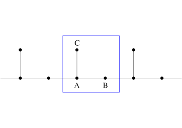
The stub chain (see figure 1, left) is the simplest of all 1D structures exhibiting a flat band [13, 14, 16]. We equip it with a tight-binding model with diagonal disorder. All hopping amplitudes between neighboring atoms equal unity. All disordered potentials vnAsuperscriptsubscript𝑣𝑛𝐴v_{n}^{A}, vnBsuperscriptsubscript𝑣𝑛𝐵v_{n}^{B}, vnCsuperscriptsubscript𝑣𝑛𝐶v_{n}^{C} are drawn from the same symmetric distribution ρ(v)𝜌𝑣\rho(v) with variance v2=w2delimited-⟨⟩superscript𝑣2superscript𝑤2\langle v^{2}\rangle=w^{2}. The tight-binding equations at energy E𝐸E read

(EvnA)ψnA𝐸superscriptsubscript𝑣𝑛𝐴superscriptsubscript𝜓𝑛𝐴\displaystyle(E-v_{n}^{A})\psi_{n}^{A} =\displaystyle= ψn1B+ψnB+ψnC,superscriptsubscript𝜓𝑛1𝐵superscriptsubscript𝜓𝑛𝐵superscriptsubscript𝜓𝑛𝐶\displaystyle\psi_{n-1}^{B}+\psi_{n}^{B}+\psi_{n}^{C},
(EvnB)ψnB𝐸superscriptsubscript𝑣𝑛𝐵superscriptsubscript𝜓𝑛𝐵\displaystyle(E-v_{n}^{B})\psi_{n}^{B} =\displaystyle= ψnA+ψn+1A,superscriptsubscript𝜓𝑛𝐴superscriptsubscript𝜓𝑛1𝐴\displaystyle\psi_{n}^{A}+\psi_{n+1}^{A},
(EvnC)ψnC𝐸superscriptsubscript𝑣𝑛𝐶superscriptsubscript𝜓𝑛𝐶\displaystyle(E-v_{n}^{C})\psi_{n}^{C} =\displaystyle= ψnA.superscriptsubscript𝜓𝑛𝐴\displaystyle\psi_{n}^{A}. (3.1)
Refer to caption
Refer to caption
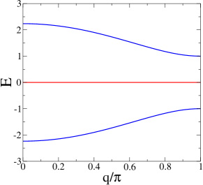
Figure 1: Left: the stub chain has 3 atoms per unit cell. Right: its spectrum (see (3.3)) has one central flat band (red) isolated from two symmetric dispersive ones (blue).

The dispersion relation of a clean stub chain is obtained by expressing that E𝐸E is an eigenvalue of the matrix

M(q)=(01+iq11+iq00100)𝑀𝑞matrix01superscripti𝑞11superscripti𝑞00100M(q)=\pmatrix{0&1+\rme^{-{\rm i}q}&1\cr 1+\rme^{{\rm i}q}&0&0\cr 1&0&0} (3.2)

encoding the right-hand sides of (3.1). The spectrum (see figure 1, right) consists of one flat band and two dispersive bands:

E𝐸\displaystyle E =\displaystyle= 0,0\displaystyle 0,
E𝐸\displaystyle E =\displaystyle= ±3+2cosq.plus-or-minus32𝑞\displaystyle\pm\sqrt{3+2\cos q}. (3.3)

The flat band is isolated, i.e., separated from the dispersive ones by a finite gap ΔE=1Δ𝐸1\Delta E=1. It consists of the extensively degenerate states

ψnB=σn,ψnC=σn1+σn,formulae-sequencesuperscriptsubscript𝜓𝑛𝐵subscript𝜎𝑛superscriptsubscript𝜓𝑛𝐶subscript𝜎𝑛1subscript𝜎𝑛\psi_{n}^{B}=-\sigma_{n},\qquad\psi_{n}^{C}=\sigma_{n-1}+\sigma_{n}, (3.4)

where σnsubscript𝜎𝑛\sigma_{n} are arbitrary amplitudes. The most localized states, corresponding e.g. to σn=δn0subscript𝜎𝑛subscript𝛿𝑛0\sigma_{n}=\delta_{n0}, live on three sites belonging to two consecutive cells, such as e.g. B0subscript𝐵0B_{0}, C0subscript𝐶0C_{0} and C1subscript𝐶1C_{1}.

In the presence of a weak disorder, the flat band is broadened symmetrically over an energy range of order w𝑤w. If the disorder distribution is supported by a finite interval, i.e., ρ(v)𝜌𝑣\rho(v) is non-zero only for |v|<V𝑣𝑉|v|<V, the disordered flat band has well-defined edges at E=±V𝐸plus-or-minus𝑉E=\pm V. The density of states vanishes exponentially fast in the vicinity of these band edges, which correspond to internal Lifshitz tails [32, 33]. For V<1/2𝑉12V<1/2, the disordered flat band remains isolated from the dispersive ones. For the uniform distribution on [V,V]𝑉𝑉[-V,V], with w2=V2/3superscript𝑤2superscript𝑉23w^{2}=V^{2}/3, the band edges read E=±w3𝐸plus-or-minus𝑤3E=\pm w\sqrt{3}.

The weakly disordered flat band of the stub lattice has been investigated in several recent works [13, 14, 16]. The subsequent analysis corroborates earlier findings and allows us to make more precise statements on some aspects.

Whenever energy E𝐸E and all disordered potentials are simultaneously small, the tight-binding equations (3.1) simplify to

ψn+1Asuperscriptsubscript𝜓𝑛1𝐴\displaystyle\psi_{n+1}^{A} \displaystyle\approx ψnA+ηnϕnB,superscriptsubscript𝜓𝑛𝐴subscript𝜂𝑛superscriptsubscriptitalic-ϕ𝑛𝐵\displaystyle-\psi_{n}^{A}+\eta_{n}\phi_{n}^{B},
ϕn+1Bsuperscriptsubscriptitalic-ϕ𝑛1𝐵\displaystyle\phi_{n+1}^{B} \displaystyle\approx ϕnBχnψn+1A,superscriptsubscriptitalic-ϕ𝑛𝐵subscript𝜒𝑛superscriptsubscript𝜓𝑛1𝐴\displaystyle-\phi_{n}^{B}-\chi_{n}\psi_{n+1}^{A}, (3.5)

where the amplitudes ψnCsuperscriptsubscript𝜓𝑛𝐶\psi_{n}^{C} have been eliminated, the rescaling ϕnB=EψnBsuperscriptsubscriptitalic-ϕ𝑛𝐵𝐸superscriptsubscript𝜓𝑛𝐵\phi_{n}^{B}=E\psi_{n}^{B} has been done, and

ηn=1vnBE,χn=(1vnCE)1formulae-sequencesubscript𝜂𝑛1superscriptsubscript𝑣𝑛𝐵𝐸subscript𝜒𝑛superscript1superscriptsubscript𝑣𝑛𝐶𝐸1\eta_{n}=1-\frac{v_{n}^{B}}{E},\qquad\chi_{n}=\left(1-\frac{v_{n}^{C}}{E}\right)^{-1} (3.6)

are reduced disorder variables. Furthermore, the rescaled equations (3.5) can be recast as a product of 2×2222\times 2 independent random matrices, namely

(ψn+1Aϕn+1B)Tn(ψnAϕnB),matrixsuperscriptsubscript𝜓𝑛1𝐴superscriptsubscriptitalic-ϕ𝑛1𝐵subscript𝑇𝑛matrixsuperscriptsubscript𝜓𝑛𝐴superscriptsubscriptitalic-ϕ𝑛𝐵\pmatrix{\psi_{n+1}^{A}\cr\phi_{n+1}^{B}}\approx T_{n}\pmatrix{\psi_{n}^{A}\cr\phi_{n}^{B}}, (3.7)

with

Tn=(1ηnχn1+ηnχn).subscript𝑇𝑛matrix1subscript𝜂𝑛subscript𝜒𝑛1subscript𝜂𝑛subscript𝜒𝑛T_{n}=-\pmatrix{1&-\eta_{n}\cr-\chi_{n}&1+\eta_{n}\chi_{n}}. (3.8)

We have again detTn=1subscript𝑇𝑛1\det T_{n}=1. The associated Riccati variables obey the recursion

Rn+1=Rnηn1+χn(ηnRn).subscript𝑅𝑛1subscript𝑅𝑛subscript𝜂𝑛1subscript𝜒𝑛subscript𝜂𝑛subscript𝑅𝑛R_{n+1}=\frac{R_{n}-\eta_{n}}{1+\chi_{n}(\eta_{n}-R_{n})}. (3.9)

The associated Lyapunov exponent

γ=ln|RnηnRn|𝛾delimited-⟨⟩subscript𝑅𝑛subscript𝜂𝑛subscript𝑅𝑛\gamma=\left\langle\ln\left|\frac{R_{n}-\eta_{n}}{R_{n}}\right|\right\rangle (3.10)

gives the inverse localization length, in units of the size of a unit cell.

The above formalism involves E𝐸E only through the dimensionless quantities ηnsubscript𝜂𝑛\eta_{n} and χnsubscript𝜒𝑛\chi_{n}. As a consequence, the Lyapunov exponent depends on energy only through the dimensionless ratio [14, 16]

x=Ew.𝑥𝐸𝑤x=\frac{E}{w}. (3.11)

In the absence of disorder (ηn=χn=1subscript𝜂𝑛subscript𝜒𝑛1\eta_{n}=\chi_{n}=1), the recursion (3.9) has two fixed points, R+subscript𝑅R_{+} (unstable) and Rsubscript𝑅R_{-} (stable), with R±=(1±5)/2subscript𝑅plus-or-minusplus-or-minus152R_{\pm}=(1\pm\sqrt{5})/2. The associated Lyapunov exponent is γ=ln(11/R)subscript𝛾11subscript𝑅\gamma_{\infty}=\ln(1-1/R_{-}), i.e.,

γ=ln3+52=0.962423.subscript𝛾3520.962423\gamma_{\infty}=\ln\frac{3+\sqrt{5}}{2}=0.962423. (3.12)

This is the value of the inverse localization length for w|E|1much-less-than𝑤𝐸much-less-than1w\ll|E|\ll 1, i.e., |x|1much-greater-than𝑥1|x|\gg 1. This result can be recovered by more elementary means, along the lines of [16]. The pristine chain has extensively degenerate states given by (3.4). An infinitesimal disorder lifts this extensive degeneracy by allowing the flat-band states to hybridize with the dispersive ones. Setting E=0𝐸0E=0 in the expression (3.3) of the dispersive bands yields a complex momentum qsubscript𝑞q_{\star} such that cosq=3/2subscript𝑞32\cos q_{\star}=-3/2, i.e., iq=(3±5)/2superscriptisubscript𝑞plus-or-minus352\rme^{{\rm i}q_{\star}}=-(3\pm\sqrt{5})/2. The latter momentum describes the falloff of flat-band states in the limit of an infinitesimal disorder. The identification |Imq|=γImsubscript𝑞subscript𝛾|\mathop{\rm Im}\,q_{\star}|=\gamma_{\infty} allows one to recover (3.12).

A systematic weak-disorder expansion around (3.12) can be derived by considering the variables

Zn=RnRRnR+,subscript𝑍𝑛subscript𝑅𝑛subscript𝑅subscript𝑅𝑛subscript𝑅Z_{n}=\frac{R_{n}-R_{-}}{R_{n}-R_{+}}, (3.13)

which represent the deviation of the Riccati variables from the stable fixed point, and are therefore small at weak disorder. The Znsubscript𝑍𝑛Z_{n} obey the recursion

Zn+1=Nn+1Dn+1,subscript𝑍𝑛1subscript𝑁𝑛1subscript𝐷𝑛1Z_{n+1}=\frac{N_{n+1}}{D_{n+1}}, (3.14)

with

Nn+1subscript𝑁𝑛1\displaystyle N_{n+1} =\displaystyle= (55+(15)vnB+4vnC+(1+5)vnBvnC)(Zn1)5515superscriptsubscript𝑣𝑛𝐵4superscriptsubscript𝑣𝑛𝐶15superscriptsubscript𝑣𝑛𝐵superscriptsubscript𝑣𝑛𝐶subscript𝑍𝑛1\displaystyle\left(\sqrt{5}-5+(1-\sqrt{5})v_{n}^{B}+4v_{n}^{C}+(1+\sqrt{5})v_{n}^{B}v_{n}^{C}\right)\!(Z_{n}-1)
+\displaystyle+ 55+(5+5)vnC,5555superscriptsubscript𝑣𝑛𝐶\displaystyle\sqrt{5}-5+(5+\sqrt{5})v_{n}^{C},
Dn+1subscript𝐷𝑛1\displaystyle D_{n+1} =\displaystyle= ((4+25)vnB(1+5)vnC+(1+5)vnBvnC)(Zn1)425superscriptsubscript𝑣𝑛𝐵15superscriptsubscript𝑣𝑛𝐶15superscriptsubscript𝑣𝑛𝐵superscriptsubscript𝑣𝑛𝐶subscript𝑍𝑛1\displaystyle\left(-(4+2\sqrt{5})v_{n}^{B}-(1+\sqrt{5})v_{n}^{C}+(1+\sqrt{5})v_{n}^{B}v_{n}^{C}\right)\!(Z_{n}-1) (3.15)
\displaystyle- 4510+(5+5)vnC,451055superscriptsubscript𝑣𝑛𝐶\displaystyle 4\sqrt{5}-10+(5+\sqrt{5})v_{n}^{C},

whereas (3.10) reads

γ=ln|1+(5+1)(1vnB)(1Zn)2+(3+5)Zn|.𝛾delimited-⟨⟩1511superscriptsubscript𝑣𝑛𝐵1subscript𝑍𝑛235subscript𝑍𝑛\gamma=\left\langle\ln\left|1+(\sqrt{5}+1)\frac{(1-v_{n}^{B})(1-Z_{n})}{2+(3+\sqrt{5})Z_{n}}\right|\right\rangle. (3.16)

Expanding the recursion (3.14) in powers of the disordered potentials allows one to derive a weak-disorder expansion of the moments of the invariant distribution of Z𝑍Z. We thus obtain

Z=5+550v2E2+29575250v4E4+27125125v22E4+delimited-⟨⟩𝑍5550delimited-⟨⟩superscript𝑣2superscript𝐸229575250delimited-⟨⟩superscript𝑣4superscript𝐸427125125superscriptdelimited-⟨⟩superscript𝑣22superscript𝐸4\langle Z\rangle=-\frac{5+\sqrt{5}}{50}\frac{\langle v^{2}\rangle}{E^{2}}+\frac{29\sqrt{5}-75}{250}\frac{\langle v^{4}\rangle}{E^{4}}+\frac{27-12\sqrt{5}}{125}\frac{\langle v^{2}\rangle^{2}}{E^{4}}+\cdots (3.17)

and analogous expressions for Zpdelimited-⟨⟩superscript𝑍𝑝\langle Z^{p}\rangle for p=2𝑝2p=2, 3 and 4. Putting everything together, we obtain a fourth-order expansion of the Lyapunov exponent. Once recast in terms of the reduced quantities x𝑥x (see (3.11)) and κ=v4/w4𝜅delimited-⟨⟩superscript𝑣4superscript𝑤4\kappa=\langle v^{4}\rangle/w^{4}, the kurtosis of the disorder distribution, the latter expansion appears as a large-x𝑥x expansion:

γ=γ+515x2+(658)κ+53525x4+𝛾subscript𝛾515superscript𝑥2658𝜅53525superscript𝑥4\gamma=\gamma_{\infty}+\frac{\sqrt{5}-1}{5\,x^{2}}+\frac{(6\sqrt{5}-8)\kappa+5-3\sqrt{5}}{25\,x^{4}}+\cdots (3.18)

Higher-order dimensionless ratios such as κp=v2p/w2psubscript𝜅𝑝delimited-⟨⟩superscript𝑣2𝑝superscript𝑤2𝑝\kappa_{p}=\langle v^{2p}\rangle/w^{2p} for p=3,4,𝑝34p=3,4,\dots enter higher-order terms of the above expansion. This demonstrates that the Lyapunov exponent depends on all moments of the disorder distribution, i.e., on its full shape, and not only on the disorder width w𝑤w.

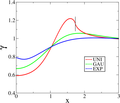
Besides the above expansion, no analytical result is available in general. In order to proceed, we must have recourse to a numerical study. A very efficient approach consists in building up the invariant measure by iterating the rescaled recursion (3.9) along a very long trajectory (e.g. of length 108superscript10810^{8}). Figure 2 shows the Lyapunov exponent thus obtained. Throughout this work, we compare results for three disorder distributions: uniform, Gaussian and exponential (see B.3 for details).
Refer to caption
Figure 2: The Lyapunov exponent γ𝛾\gamma against reduced energy x=E/w𝑥𝐸𝑤x=E/w for three disorder distributions: uniform, Gaussian and exponential. Vertical segment: edge of flat band for the uniform distribution (x=3𝑥3x=\sqrt{3}).

The Lyapunov exponent (inverse localization length) is an even smooth function of the reduced energy x𝑥x (see (3.11)), which depends on the shape of the disorder distribution. It exhibits a non-monotonic dependence on the reduced energy, with a non-trivial maximum γmaxsubscript𝛾max\gamma_{\rm max}, put forward in Reference [16] as an anomalous minimum localization length. For large x𝑥x, it approaches the limit γsubscript𝛾\gamma_{\infty} from above, according to the expansion (3.18), which also predicts the observed ordering of the curves at large x𝑥x. The coefficient of the kurtosis κ𝜅\kappa in (3.18) is positive, and the curves are indeed ordered as the kurtosis of the distributions, which are recalled in table 1 below. For the uniform distribution, the disordered flat band exhibits a band edge at x=3𝑥3x=\sqrt{3}, shown as a vertical segment. The Lyapunov exponent reaches its maximum within the band but not far from the band edge. It seems to have only a very mild singularity there, in agreement with the Lifshitz behavior of the density of states recalled above. The Lyapunov exponent often reaches its minimum at the band center (γmin=γ(0)subscript𝛾min𝛾0\gamma_{\rm min}=\gamma(0)), in agreement with the intuitive picture that the states closest to the band center are the most hybridized, so that their localization length is the largest. This is however not true for the exponential distribution, where the Lyapunov exponent exhibits a non-trivial minimum γminsubscript𝛾min\gamma_{\rm min} slightly below γ(0)𝛾0\gamma(0). All the characteristic values mentioned above depend on the shape of the disorder distribution (see table 1). The numbers for uniform and Gaussian disorders agree with those to be read off from the figures of [16]. Finally, for the distributions we have considered, all these quantities are monotonic functions of the kurtosis κ𝜅\kappa.

Distribution κ𝜅\kappa γmaxsubscript𝛾max\gamma_{\rm max} γ(0)𝛾0\gamma(0) γminsubscript𝛾min\gamma_{\rm min}
Uniform 1.8 1.219 0.591
Gaussian 3 1.057 0.668
Exponential 6 1.006 0.788 0.771
Table 1: Characteristic values of the Lyapunov exponent (inverse localization length) of the weakly disordered flat band of the stub lattice for three disorder distributions, whose kurtosis κ𝜅\kappa is recalled (see B.3 for details). The minimum γminsubscript𝛾min\gamma_{\rm min} is given when it is non-trivial, i.e., different from γ(0)𝛾0\gamma(0).

4 The pyrochlore ladder

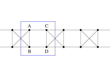
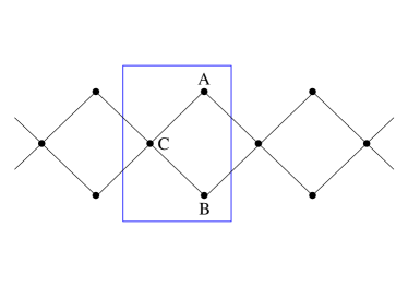
The pyrochlore ladder (see figure 3, left) is a well-known example of a 1D structure exhibiting flat bands [13, 14]. We equip it with a tight-binding model with diagonal disorder. All disordered potentials are again drawn from the same distribution. The tight-binding equations at energy E𝐸E read

(EvnA)ψnA𝐸superscriptsubscript𝑣𝑛𝐴superscriptsubscript𝜓𝑛𝐴\displaystyle(E-v_{n}^{A})\psi_{n}^{A} =\displaystyle= ψn1C+ψn1D+ψnB+ψnC,superscriptsubscript𝜓𝑛1𝐶superscriptsubscript𝜓𝑛1𝐷superscriptsubscript𝜓𝑛𝐵superscriptsubscript𝜓𝑛𝐶\displaystyle\psi_{n-1}^{C}+\psi_{n-1}^{D}+\psi_{n}^{B}+\psi_{n}^{C},
(EvnB)ψnB𝐸superscriptsubscript𝑣𝑛𝐵superscriptsubscript𝜓𝑛𝐵\displaystyle(E-v_{n}^{B})\psi_{n}^{B} =\displaystyle= ψn1C+ψn1D+ψnA+ψnD,superscriptsubscript𝜓𝑛1𝐶superscriptsubscript𝜓𝑛1𝐷superscriptsubscript𝜓𝑛𝐴superscriptsubscript𝜓𝑛𝐷\displaystyle\psi_{n-1}^{C}+\psi_{n-1}^{D}+\psi_{n}^{A}+\psi_{n}^{D},
(EvnC)ψnC𝐸superscriptsubscript𝑣𝑛𝐶superscriptsubscript𝜓𝑛𝐶\displaystyle(E-v_{n}^{C})\psi_{n}^{C} =\displaystyle= ψnA+ψnD+ψn+1A+ψn+1B,superscriptsubscript𝜓𝑛𝐴superscriptsubscript𝜓𝑛𝐷superscriptsubscript𝜓𝑛1𝐴superscriptsubscript𝜓𝑛1𝐵\displaystyle\psi_{n}^{A}+\psi_{n}^{D}+\psi_{n+1}^{A}+\psi_{n+1}^{B},
(EvnD)ψnD𝐸superscriptsubscript𝑣𝑛𝐷superscriptsubscript𝜓𝑛𝐷\displaystyle(E-v_{n}^{D})\psi_{n}^{D} =\displaystyle= ψnB+ψnC+ψn+1A+ψn+1B.superscriptsubscript𝜓𝑛𝐵superscriptsubscript𝜓𝑛𝐶superscriptsubscript𝜓𝑛1𝐴superscriptsubscript𝜓𝑛1𝐵\displaystyle\psi_{n}^{B}+\psi_{n}^{C}+\psi_{n+1}^{A}+\psi_{n+1}^{B}. (4.1)
Refer to caption
Refer to caption
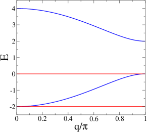
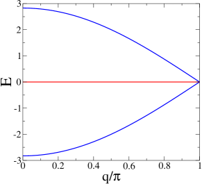
Figure 3: Left: the pyrochlore ladder has 4 atoms per unit cell. Right: its spectrum (see (4.3)) has two flat bands (red) and two dispersive ones (blue).

The dispersion relation of a clean ladder is obtained by expressing that E𝐸E is an eigenvalue of the matrix

M(q)=(011+iqiq10iq1+iq1+iqiq01iq1+iq10).𝑀𝑞matrix011superscripti𝑞superscripti𝑞10superscripti𝑞1superscripti𝑞1superscripti𝑞superscripti𝑞01superscripti𝑞1superscripti𝑞10M(q)=\pmatrix{0&1&1+\rme^{-{\rm i}q}&\rme^{-{\rm i}q}\cr 1&0&\rme^{-{\rm i}q}&1+\rme^{-{\rm i}q}\cr 1+\rme^{{\rm i}q}&\rme^{{\rm i}q}&0&1\cr\rme^{{\rm i}q}&1+\rme^{{\rm i}q}&1&0}. (4.2)

The spectrum (see figure 3, right) consists of two flat bands and two dispersive ones:

E𝐸\displaystyle E =\displaystyle= 0,0\displaystyle 0,
E𝐸\displaystyle E =\displaystyle= 2,2\displaystyle-2,
E𝐸\displaystyle E =\displaystyle= 1±5+4cosq.plus-or-minus154𝑞\displaystyle 1\pm\sqrt{5+4\cos q}. (4.3)

The lower dispersive band touches both flat bands. The latter consist of the extensively degenerate states

E=0:ψnA=ψnC=σn,ψnB=ψnD=σn,\displaystyle E=0:\hskip 32.5pt\psi_{n}^{A}=\psi_{n}^{C}=\sigma_{n},\quad\psi_{n}^{B}=\psi_{n}^{D}=-\sigma_{n},
E=2:ψnA=ψnD=τn,ψnB=ψnC=τn,\displaystyle E=-2:\qquad\psi_{n}^{A}=\psi_{n}^{D}=\tau_{n},\quad\psi_{n}^{B}=\psi_{n}^{C}=-\tau_{n}, (4.4)

where σnsubscript𝜎𝑛\sigma_{n} and τnsubscript𝜏𝑛\tau_{n} are arbitrary amplitudes. The most localized states, corresponding e.g. to σn=δn0subscript𝜎𝑛subscript𝛿𝑛0\sigma_{n}=\delta_{n0} or τn=δn0subscript𝜏𝑛subscript𝛿𝑛0\tau_{n}=\delta_{n0}, live on the four sites of a single unit cell.

The weakly disordered flat bands of the pyrochlore ladder have been investigated recently [13, 14]. Here, at variance with the case of the stub chain, a dispersive band touches both flat bands, so that the localization length is expected to be large when disorder is weak. From a quantitative viewpoint, a scaling of the localization length in w1/2superscript𝑤12w^{-1/2} is predicted in References [13, 14], based on the occurrence of an effective Cauchy disorder. The subsequent analysis corroborates this finding, provides an exact mapping onto the Lloyd model at weak disorder and yields the analytical prediction (4.23) for the corresponding non-universal scaling function F(pyro)(x)superscript𝐹pyro𝑥F^{\rm(pyro)}(x).

Let us focus our attention onto the flat band at E=0𝐸0E=0 and introduce the combinations

snsubscript𝑠𝑛\displaystyle s_{n} =\displaystyle= ψnA+ψnB+ψnC+ψnD,superscriptsubscript𝜓𝑛𝐴superscriptsubscript𝜓𝑛𝐵superscriptsubscript𝜓𝑛𝐶superscriptsubscript𝜓𝑛𝐷\displaystyle\psi_{n}^{A}+\psi_{n}^{B}+\psi_{n}^{C}+\psi_{n}^{D},
tnsubscript𝑡𝑛\displaystyle t_{n} =\displaystyle= ψnA+ψnBψnCψnD,superscriptsubscript𝜓𝑛𝐴superscriptsubscript𝜓𝑛𝐵superscriptsubscript𝜓𝑛𝐶superscriptsubscript𝜓𝑛𝐷\displaystyle\psi_{n}^{A}+\psi_{n}^{B}-\psi_{n}^{C}-\psi_{n}^{D},
unsubscript𝑢𝑛\displaystyle u_{n} =\displaystyle= ψnAψnB+ψnCψnD,superscriptsubscript𝜓𝑛𝐴superscriptsubscript𝜓𝑛𝐵superscriptsubscript𝜓𝑛𝐶superscriptsubscript𝜓𝑛𝐷\displaystyle\psi_{n}^{A}-\psi_{n}^{B}+\psi_{n}^{C}-\psi_{n}^{D},
vnsubscript𝑣𝑛\displaystyle v_{n} =\displaystyle= ψnAψnBψnC+ψnD.superscriptsubscript𝜓𝑛𝐴superscriptsubscript𝜓𝑛𝐵superscriptsubscript𝜓𝑛𝐶superscriptsubscript𝜓𝑛𝐷\displaystyle\psi_{n}^{A}-\psi_{n}^{B}-\psi_{n}^{C}+\psi_{n}^{D}. (4.5)

In the absence of disorder, the tight-binding equations (4.1) imply that snsubscript𝑠𝑛s_{n} and tnsubscript𝑡𝑛t_{n} obey the recursion

sn+1=tnsn,subscript𝑠𝑛1subscript𝑡𝑛subscript𝑠𝑛\displaystyle s_{n+1}=t_{n}-s_{n},
tn+1=tn,subscript𝑡𝑛1subscript𝑡𝑛\displaystyle t_{n+1}=-t_{n}, (4.6)

while vnsubscript𝑣𝑛v_{n} vanishes and unsubscript𝑢𝑛u_{n} is left arbitrary. The latter property is expected, as un=4σnsubscript𝑢𝑛4subscript𝜎𝑛u_{n}=4\sigma_{n} describes the compactly localized states on the pristine ladder (see (4.4)).

The idea of the subsequent analysis is to follow how the recursion (4.6), involving two variables only, is deformed when energy E𝐸E and all random potentials are simultaneously small. A careful treatment of the tight-binding equations (4.1) to first order in the variables

ηnA=EvnA,ηnB=EvnB,ηnC=EvnC,ηnD=EvnDformulae-sequencesuperscriptsubscript𝜂𝑛𝐴𝐸superscriptsubscript𝑣𝑛𝐴formulae-sequencesuperscriptsubscript𝜂𝑛𝐵𝐸superscriptsubscript𝑣𝑛𝐵formulae-sequencesuperscriptsubscript𝜂𝑛𝐶𝐸superscriptsubscript𝑣𝑛𝐶superscriptsubscript𝜂𝑛𝐷𝐸superscriptsubscript𝑣𝑛𝐷\eta_{n}^{A}=E-v_{n}^{A},\quad\eta_{n}^{B}=E-v_{n}^{B},\quad\eta_{n}^{C}=E-v_{n}^{C},\quad\eta_{n}^{D}=E-v_{n}^{D} (4.7)

yields

(sn+1tn+1)Mn(sntn),matrixsubscript𝑠𝑛1subscript𝑡𝑛1subscript𝑀𝑛matrixsubscript𝑠𝑛subscript𝑡𝑛\pmatrix{s_{n+1}\cr t_{n+1}}\approx M_{n}\pmatrix{s_{n}\cr t_{n}}, (4.8)

with

Mnsubscript𝑀𝑛\displaystyle M_{n} =\displaystyle= (1αn+11+αn+1βn+1γn+αn+11δn+βn+1αn+1)matrix1subscript𝛼𝑛11subscript𝛼𝑛1subscript𝛽𝑛1subscript𝛾𝑛subscript𝛼𝑛11subscript𝛿𝑛subscript𝛽𝑛1subscript𝛼𝑛1\displaystyle\pmatrix{-1-\alpha_{n+1}&1+\alpha_{n+1}-\beta_{n+1}\cr\gamma_{n}+\alpha_{n+1}&-1-\delta_{n}+\beta_{n+1}-\alpha_{n+1}} (4.9)
\displaystyle\approx (1αn+11+αn+1βn+1αn+11+βn+1αn+1)(1γnδnγn1+δn)matrix1subscript𝛼𝑛11subscript𝛼𝑛1subscript𝛽𝑛1subscript𝛼𝑛11subscript𝛽𝑛1subscript𝛼𝑛1matrix1subscript𝛾𝑛subscript𝛿𝑛subscript𝛾𝑛1subscript𝛿𝑛\displaystyle\pmatrix{-1-\alpha_{n+1}&1+\alpha_{n+1}-\beta_{n+1}\cr\alpha_{n+1}&-1+\beta_{n+1}-\alpha_{n+1}}\pmatrix{1-\gamma_{n}&\delta_{n}\cr-\gamma_{n}&1+\delta_{n}}

and

αn=1Δn(2ηnAηnB+ηnAηnD+ηnBηnC),subscript𝛼𝑛1subscriptΔ𝑛2superscriptsubscript𝜂𝑛𝐴superscriptsubscript𝜂𝑛𝐵superscriptsubscript𝜂𝑛𝐴superscriptsubscript𝜂𝑛𝐷superscriptsubscript𝜂𝑛𝐵superscriptsubscript𝜂𝑛𝐶\displaystyle\alpha_{n}=\frac{1}{\Delta_{n}}(2\eta_{n}^{A}\eta_{n}^{B}+\eta_{n}^{A}\eta_{n}^{D}+\eta_{n}^{B}\eta_{n}^{C}),
βn=1Δn(2ηnAηnB+ηnAηnC+ηnBηnD),subscript𝛽𝑛1subscriptΔ𝑛2superscriptsubscript𝜂𝑛𝐴superscriptsubscript𝜂𝑛𝐵superscriptsubscript𝜂𝑛𝐴superscriptsubscript𝜂𝑛𝐶superscriptsubscript𝜂𝑛𝐵superscriptsubscript𝜂𝑛𝐷\displaystyle\beta_{n}=\frac{1}{\Delta_{n}}(2\eta_{n}^{A}\eta_{n}^{B}+\eta_{n}^{A}\eta_{n}^{C}+\eta_{n}^{B}\eta_{n}^{D}),
γn=1Δn(2ηnCηnD+ηnAηnD+ηnBηnC),subscript𝛾𝑛1subscriptΔ𝑛2superscriptsubscript𝜂𝑛𝐶superscriptsubscript𝜂𝑛𝐷superscriptsubscript𝜂𝑛𝐴superscriptsubscript𝜂𝑛𝐷superscriptsubscript𝜂𝑛𝐵superscriptsubscript𝜂𝑛𝐶\displaystyle\gamma_{n}=\frac{1}{\Delta_{n}}(2\eta_{n}^{C}\eta_{n}^{D}+\eta_{n}^{A}\eta_{n}^{D}+\eta_{n}^{B}\eta_{n}^{C}),
δn=1Δn(2ηnCηnD+ηnAηnC+ηnBηnD),subscript𝛿𝑛1subscriptΔ𝑛2superscriptsubscript𝜂𝑛𝐶superscriptsubscript𝜂𝑛𝐷superscriptsubscript𝜂𝑛𝐴superscriptsubscript𝜂𝑛𝐶superscriptsubscript𝜂𝑛𝐵superscriptsubscript𝜂𝑛𝐷\displaystyle\delta_{n}=\frac{1}{\Delta_{n}}(2\eta_{n}^{C}\eta_{n}^{D}+\eta_{n}^{A}\eta_{n}^{C}+\eta_{n}^{B}\eta_{n}^{D}), (4.10)

with

Δn=2(ηnA+ηnB+ηnC+ηnD).subscriptΔ𝑛2superscriptsubscript𝜂𝑛𝐴superscriptsubscript𝜂𝑛𝐵superscriptsubscript𝜂𝑛𝐶superscriptsubscript𝜂𝑛𝐷\Delta_{n}=2(\eta_{n}^{A}+\eta_{n}^{B}+\eta_{n}^{C}+\eta_{n}^{D}). (4.11)

We have αn+δn=βn+γnsubscript𝛼𝑛subscript𝛿𝑛subscript𝛽𝑛subscript𝛾𝑛\alpha_{n}+\delta_{n}=\beta_{n}+\gamma_{n}.

In the weak-disorder regime, the Lyapunov exponent of the above matrix product can be determined by means of an exact mapping onto the Lloyd model (see section 2.3). The mapping proceeds in two steps. First, the transfer matrices Mnsubscript𝑀𝑛M_{n} are not independent from each other, as they involve the disordered potentials in two neighboring cells. This can be remedied by swapping both matrices entering the second line of (4.9), i.e., by replacing Mnsubscript𝑀𝑛M_{n} by

M~nsubscript~𝑀𝑛\displaystyle\widetilde{M}_{n} =\displaystyle= (1γnδnγn1+δn)(1αn1+αnβnαn1+βnαn)matrix1subscript𝛾𝑛subscript𝛿𝑛subscript𝛾𝑛1subscript𝛿𝑛matrix1subscript𝛼𝑛1subscript𝛼𝑛subscript𝛽𝑛subscript𝛼𝑛1subscript𝛽𝑛subscript𝛼𝑛\displaystyle-\pmatrix{1-\gamma_{n}&\delta_{n}\cr-\gamma_{n}&1+\delta_{n}}\pmatrix{-1-\alpha_{n}&1+\alpha_{n}-\beta_{n}\cr\alpha_{n}&-1+\beta_{n}-\alpha_{n}} (4.12)
\displaystyle\approx (1+an1+cnbn1+dn),matrix1subscript𝑎𝑛1subscript𝑐𝑛subscript𝑏𝑛1subscript𝑑𝑛\displaystyle\pmatrix{1+a_{n}&-1+c_{n}\cr b_{n}&1+d_{n}},

to leading order, with

an=αnγn,bn=αnγn,cn=2δn,dn=2γn.formulae-sequencesubscript𝑎𝑛subscript𝛼𝑛subscript𝛾𝑛formulae-sequencesubscript𝑏𝑛subscript𝛼𝑛subscript𝛾𝑛formulae-sequencesubscript𝑐𝑛2subscript𝛿𝑛subscript𝑑𝑛2subscript𝛾𝑛a_{n}=\alpha_{n}-\gamma_{n},\quad b_{n}=-\alpha_{n}-\gamma_{n},\quad c_{n}=2\delta_{n},\quad d_{n}=2\gamma_{n}. (4.13)

We have an+bn+dn=0subscript𝑎𝑛subscript𝑏𝑛subscript𝑑𝑛0a_{n}+b_{n}+d_{n}=0, and so detM~n=1subscript~𝑀𝑛1\det\widetilde{M}_{n}=1, to leading order. A minus sign has been introduced for convenience in the definition of M~nsubscript~𝑀𝑛\widetilde{M}_{n}. Second, a change of basis defined by the matrix

P=(1011)𝑃matrix1011P=\pmatrix{1&0\cr-1&1} (4.14)

amounts to replacing M~nsubscript~𝑀𝑛\widetilde{M}_{n} by

Tn=P1M~nP(2+ancn1+cn1cn2dncn+dn).subscript𝑇𝑛superscript𝑃1subscript~𝑀𝑛𝑃matrix2subscript𝑎𝑛subscript𝑐𝑛1subscript𝑐𝑛1subscript𝑐𝑛2subscript𝑑𝑛subscript𝑐𝑛subscript𝑑𝑛T_{n}=P^{-1}\widetilde{M}_{n}P\approx\pmatrix{2+a_{n}-c_{n}&-1+c_{n}\cr 1-c_{n}-2d_{n}&c_{n}+d_{n}}. (4.15)

At weak disorder, the above transfer matrix is close to that of the Anderson model on the chain, given by (2.4), near the upper band edge (E2𝐸2E\approx 2). The Riccati variables associated with (4.15) obey the recursion

Rn=(2+ancn)Rn11+cn(1cn2dn)Rn1+cn+dn.subscript𝑅𝑛2subscript𝑎𝑛subscript𝑐𝑛subscript𝑅𝑛11subscript𝑐𝑛1subscript𝑐𝑛2subscript𝑑𝑛subscript𝑅𝑛1subscript𝑐𝑛subscript𝑑𝑛R_{n}=\frac{(2+a_{n}-c_{n})R_{n-1}-1+c_{n}}{(1-c_{n}-2d_{n})R_{n-1}+c_{n}+d_{n}}. (4.16)

Let us anticipate for a while that the disorder entering (4.15) has Cauchy tails. An appropriate identification of the random recursions (2.12) and (4.16) yields a mapping of the present problem onto the Lloyd model (see section 2.3). Let us denote quantities pertaining to the latter model with a superscript (L)L{\rm(L)}. Near the upper band edge (E(L)2superscript𝐸L2E^{\rm(L)}\approx 2) and at weak disorder, the invariant distribution f(L)(R)superscript𝑓L𝑅f^{\rm(L)}(R) is a narrow distribution concentrated around R=1𝑅1R=1. Equation (2.23) indeed shows that R=a(L)delimited-⟨⟩𝑅superscriptsubscript𝑎L\langle R\rangle=a_{\star}^{\rm(L)} is close to unity, whereas the width b(L)superscriptsubscript𝑏Lb_{\star}^{\rm(L)} scales as W(L)superscript𝑊L\sqrt{W^{\rm(L)}}. It is therefore sufficient to compare the formulas (2.12) and (4.16) in the vicinity of R=1𝑅1R=1. Both equations obey Rn/Rn11subscript𝑅𝑛subscript𝑅𝑛11\partial R_{n}/\partial R_{n-1}\approx 1 at weak disorder. Equating the values of Rnsubscript𝑅𝑛R_{n} for Rn1=1subscript𝑅𝑛11R_{n-1}=1 yields the identification

E(L)2vn(L)an+dn=αn+γn=ηn(1)ηn(2)ηn(1)+ηn(2),superscript𝐸L2superscriptsubscript𝑣𝑛Lsubscript𝑎𝑛subscript𝑑𝑛subscript𝛼𝑛subscript𝛾𝑛superscriptsubscript𝜂𝑛1superscriptsubscript𝜂𝑛2superscriptsubscript𝜂𝑛1superscriptsubscript𝜂𝑛2E^{\rm(L)}-2-v_{n}^{\rm(L)}\approx a_{n}+d_{n}=\alpha_{n}+\gamma_{n}=\frac{\eta_{n}^{(1)}\eta_{n}^{(2)}}{\eta_{n}^{(1)}+\eta_{n}^{(2)}}, (4.17)

to leading order, with

ηn(1)=ηnA+ηnC=2EvnAvnC,superscriptsubscript𝜂𝑛1superscriptsubscript𝜂𝑛𝐴superscriptsubscript𝜂𝑛𝐶2𝐸superscriptsubscript𝑣𝑛𝐴superscriptsubscript𝑣𝑛𝐶\displaystyle\eta_{n}^{(1)}=\eta_{n}^{A}+\eta_{n}^{C}=2E-v_{n}^{A}-v_{n}^{C},
ηn(2)=ηnB+ηnD=2EvnBvnD.superscriptsubscript𝜂𝑛2superscriptsubscript𝜂𝑛𝐵superscriptsubscript𝜂𝑛𝐷2𝐸superscriptsubscript𝑣𝑛𝐵superscriptsubscript𝑣𝑛𝐷\displaystyle\eta_{n}^{(2)}=\eta_{n}^{B}+\eta_{n}^{D}=2E-v_{n}^{B}-v_{n}^{D}. (4.18)

The effective disorder defined in the rightmost side of (4.17) is a homogeneous but non-linear combination of the four disordered potentials of the n𝑛nth unit cell. It is typically small at weak disorder. It may however become large in the rare instances where its denominator nearly vanishes. As a consequence, it has a broad probability distribution exhibiting symmetric Cauchy tails (see A). In the present context, this specific feature of disorder has been put forward for the first time in Reference [12]. The above effective disorder is therefore characterized by two parameters, its Cauchy strength and its mean value, namely

G2(E)=δ(ηn(1)+ηn(2)ηn(1)ηn(2)),H2(E)=ηn(1)ηn(2)ηn(1)+ηn(2).formulae-sequencesubscript𝐺2𝐸delimited-⟨⟩𝛿superscriptsubscript𝜂𝑛1superscriptsubscript𝜂𝑛2superscriptsubscript𝜂𝑛1superscriptsubscript𝜂𝑛2subscript𝐻2𝐸delimited-⟨⟩superscriptsubscript𝜂𝑛1superscriptsubscript𝜂𝑛2superscriptsubscript𝜂𝑛1superscriptsubscript𝜂𝑛2G_{2}(E)=\left\langle\delta\left(\frac{\eta_{n}^{(1)}+\eta_{n}^{(2)}}{\eta_{n}^{(1)}\eta_{n}^{(2)}}\right)\right\rangle,\qquad H_{2}(E)=\left\langle\frac{\eta_{n}^{(1)}\eta_{n}^{(2)}}{\eta_{n}^{(1)}+\eta_{n}^{(2)}}\right\rangle. (4.19)

These quantities are investigated in B.2. Their scaling dependence on w𝑤w reads (see (2.18))

G2(E)=wg2(x),H2(E)=wh2(x),x=Ew.formulae-sequencesubscript𝐺2𝐸𝑤subscript𝑔2𝑥formulae-sequencesubscript𝐻2𝐸𝑤subscript2𝑥𝑥𝐸𝑤G_{2}(E)=wg_{2}(x),\qquad H_{2}(E)=wh_{2}(x),\qquad x=\frac{E}{w}. (4.20)

Working out explicitly the identification (4.17) yields

W(L)πwg2(x),x(L)h2(x)πg2(x).formulae-sequencesuperscript𝑊L𝜋𝑤subscript𝑔2𝑥superscript𝑥Lsubscript2𝑥𝜋subscript𝑔2𝑥W^{\rm(L)}\approx\pi wg_{2}(x),\qquad x^{\rm(L)}\approx\frac{h_{2}(x)}{\pi g_{2}(x)}. (4.21)

We finally obtain our prediction for the scaling behavior of the Lyapunov exponent of the weakly disordered flat band near E=0𝐸0E=0 by inserting the estimates (4.21) into (2.24). This reads

γw1/2F(pyro)(x),𝛾superscript𝑤12superscript𝐹pyro𝑥\gamma\approx w^{1/2}\,F^{\rm(pyro)}(x), (4.22)

where the scaling function reads

F(pyro)(x)=12(h2(x)+h2(x)2+π2g2(x)2)1/2.superscript𝐹pyro𝑥12superscriptsubscript2𝑥subscript2superscript𝑥2superscript𝜋2subscript𝑔2superscript𝑥212F^{\rm(pyro)}(x)=\frac{1}{\sqrt{2}}\left(h_{2}(x)+\sqrt{h_{2}(x)^{2}+\pi^{2}g_{2}(x)^{2}}\right)^{1/2}. (4.23)

This result simplifies right at E=0𝐸0E=0. We have h2(0)=0subscript200h_{2}(0)=0 by symmetry, and so

F(pyro)(0)=(πg2(0)2)1/2.superscript𝐹pyro0superscript𝜋subscript𝑔20212F^{\rm(pyro)}(0)=\left(\frac{\pi g_{2}(0)}{2}\right)^{1/2}. (4.24)

The scaling function F(pyro)(x)superscript𝐹pyro𝑥F^{\rm(pyro)}(x) is non-universal, as it depends on the full shape of the disorder distribution through the functions g2(x)subscript𝑔2𝑥g_{2}(x) and h2(x)subscript2𝑥h_{2}(x), investigated in B.2. For the uniform, Gaussian and exponential distributions, explicit expressions of g2(x)subscript𝑔2𝑥g_{2}(x) are given in B.3, and the values of g2(0)subscript𝑔20g_{2}(0) in table 2. The function h2(x)subscript2𝑥h_{2}(x) is expressed as an integral that can be carried out in closed form only for Gaussian disorder.

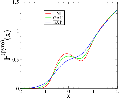
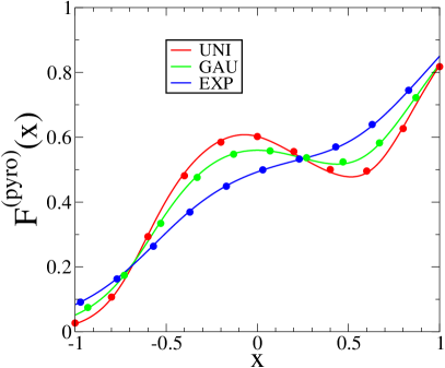
The scaling function F(pyro)(x)superscript𝐹pyro𝑥F^{\rm(pyro)}(x) is plotted in figure 4 for the uniform, Gaussian and exponential disorder distributions. The right panel, showing an enlargement of the central part of the left one, demonstrates that the analytical prediction (4.22) is in excellent agreement with numerical results for the Lyapunov exponent (symbols), based on products of 108superscript10810^{8} matrices for each type disorder with w=0.001𝑤0.001w=0.001.

Refer to caption
Refer to caption
Figure 4: Left: the non-universal scaling function F(pyro)(x)superscript𝐹pyro𝑥F^{\rm(pyro)}(x) (see (4.23)) entering the prediction (4.22) for the Lyapunov exponent of the pyrochlore ladder near E=0𝐸0E=0, against reduced energy x=E/w𝑥𝐸𝑤x=E/w, for three disorder distributions: uniform, Gaussian and exponential. Right: enlargement of the central part of the left plot. Symbols: Numerical results for w=0.001𝑤0.001w=0.001.

The most salient feature of these plots is that they are very asymmetric. It is indeed expected that the Lyapunov exponent (inverse localization length) is much smaller for x𝑥x negative, i.e., on the side of the dispersive band, than for x𝑥x positive, i.e., on the side of the gap. From a quantitative viewpoint, deep in the gap (x1much-greater-than𝑥1x\gg 1, i.e., Ewmuch-greater-than𝐸𝑤E\gg w), g2(x)subscript𝑔2𝑥g_{2}(x) falls off rapidly to zero, whereas h2(x)xsubscript2𝑥𝑥h_{2}(x)\approx x (see (2.19)). We thus obtain the universal law

F(pyro)(x)x,superscript𝐹pyro𝑥𝑥F^{\rm(pyro)}(x)\approx\sqrt{x}, (4.25)

irrespective of the disorder distribution. This collapse is clearly seen in the right part of the left panel. The formula (4.25) can be recast as γE𝛾𝐸\gamma\approx\sqrt{E}. This estimate, which does not involve disorder at all, is in agreement with the quadratic form of the lower dispersive band near E=0𝐸0E=0, i.e., E(πq)2𝐸superscript𝜋𝑞2E\approx-(\pi-q)^{2} (see (4.3)), and so γ=|Imq|E𝛾Im𝑞𝐸\gamma=|\mathop{\rm Im}\,q\,|\approx\sqrt{E}. For the uniform distribution, g2(x)subscript𝑔2𝑥g_{2}(x) vanishes identically for |x|>3𝑥3|x|>\sqrt{3} (see (2.24)). As a consequence, F(pyro)(x)superscript𝐹pyro𝑥F^{\rm(pyro)}(x) vanishes for x<3𝑥3x<-\sqrt{3}, implying that γ𝛾\gamma vanishes more rapidly than w𝑤\sqrt{w} as w𝑤w tends to zero while E<w3𝐸𝑤3E<-w\sqrt{3}. The Lyapunov exponent is indeed expected to exhibit the usual scaling in w2superscript𝑤2w^{2} at any fixed energy inside the dispersive band. In the central part, enlarged in the right panel, the scaling function F(pyro)(x)superscript𝐹pyro𝑥F^{\rm(pyro)}(x) exhibits a rather strong dependence on the disorder distribution. It is non-monotonic for the uniform and Gaussian distributions.

5 The diamond chain

The diamond chain (see figure 5, left) is another 1D structure known to exhibit a flat band [12, 14]. We equip it with a tight-binding model with diagonal disorder. All disordered potentials are again drawn from the same distribution. The tight-binding equations at energy E𝐸E read

(EvnA)ψnA𝐸superscriptsubscript𝑣𝑛𝐴superscriptsubscript𝜓𝑛𝐴\displaystyle(E-v_{n}^{A})\psi_{n}^{A} =\displaystyle= ψnC+ψn+1C,superscriptsubscript𝜓𝑛𝐶superscriptsubscript𝜓𝑛1𝐶\displaystyle\psi_{n}^{C}+\psi_{n+1}^{C},
(EvnB)ψnB𝐸superscriptsubscript𝑣𝑛𝐵superscriptsubscript𝜓𝑛𝐵\displaystyle(E-v_{n}^{B})\psi_{n}^{B} =\displaystyle= ψnC+ψn+1C,superscriptsubscript𝜓𝑛𝐶superscriptsubscript𝜓𝑛1𝐶\displaystyle\psi_{n}^{C}+\psi_{n+1}^{C},
(EvnC)ψnC𝐸superscriptsubscript𝑣𝑛𝐶superscriptsubscript𝜓𝑛𝐶\displaystyle(E-v_{n}^{C})\psi_{n}^{C} =\displaystyle= ψn1A+ψn1B+ψnA+ψnB.superscriptsubscript𝜓𝑛1𝐴superscriptsubscript𝜓𝑛1𝐵superscriptsubscript𝜓𝑛𝐴superscriptsubscript𝜓𝑛𝐵\displaystyle\psi_{n-1}^{A}+\psi_{n-1}^{B}+\psi_{n}^{A}+\psi_{n}^{B}. (5.1)
Refer to caption
Refer to caption
Figure 5: Left: the diamond chain has 3 atoms per unit cell. Right: its spectrum (see (5.3)) has one flat band (red) and two dispersive ones (blue).

The dispersion relation of a clean chain is obtained by expressing that E𝐸E is an eigenvalue of the matrix

M(q)=(001+iq001+iq1+iq1+iq0).𝑀𝑞matrix001superscripti𝑞001superscripti𝑞1superscripti𝑞1superscripti𝑞0M(q)=\pmatrix{0&0&1+\rme^{{\rm i}q}\cr 0&0&1+\rme^{{\rm i}q}\cr 1+\rme^{-{\rm i}q}&1+\rme^{-{\rm i}q}&0}. (5.2)

The spectrum (see figure 5, right) consists of one flat band and two dispersive ones:

E𝐸\displaystyle E =\displaystyle= 0,0\displaystyle 0,
E𝐸\displaystyle E =\displaystyle= ±22cosq2.plus-or-minus22𝑞2\displaystyle\pm 2\sqrt{2}\cos\frac{q}{2}. (5.3)

Both dispersive bands intersect the flat one at the edges of the Brillouin zone (q=±π)q=\pm\pi). The flat band consist of the extensively degenerate states

ψnA=ψnB=σn,superscriptsubscript𝜓𝑛𝐴superscriptsubscript𝜓𝑛𝐵subscript𝜎𝑛\displaystyle\psi_{n}^{A}=-\psi_{n}^{B}=\sigma_{n}, (5.4)

where σnsubscript𝜎𝑛\sigma_{n} are arbitrary amplitudes. The most localized states, corresponding to e.g. σn=δn0subscript𝜎𝑛subscript𝛿𝑛0\sigma_{n}=\delta_{n0}, live on two sites.

The weakly disordered flat band of the diamond chain has been investigated recently [12, 14]. Here, too, as dispersive bands intersect the flat band, the localization length is expected to be large when the disorder is weak. From a quantitative viewpoint, a scaling of the localization length in w4/3superscript𝑤43w^{-4/3} was predicted in References [12, 14]. The subsequent analysis refines this finding. We shall indeed demonstrate that the Lyapunov exponent obeys two different scaling laws in two successive regimes as energy goes away from the pristine flat band, scaling first as w4/3superscript𝑤43w^{4/3} in Regime I (Ew5/3similar-to𝐸superscript𝑤53E\sim w^{5/3}) and then as w𝑤w in Regime II (Ewsimilar-to𝐸𝑤E\sim w).

The scaling analysis of the model goes as follows. Introducing the combinations

snsubscript𝑠𝑛\displaystyle s_{n} =\displaystyle= ψnA+ψnB,superscriptsubscript𝜓𝑛𝐴superscriptsubscript𝜓𝑛𝐵\displaystyle\psi_{n}^{A}+\psi_{n}^{B},
tnsubscript𝑡𝑛\displaystyle t_{n} =\displaystyle= ψnAψnB,superscriptsubscript𝜓𝑛𝐴superscriptsubscript𝜓𝑛𝐵\displaystyle\psi_{n}^{A}-\psi_{n}^{B}, (5.5)

one can eliminate tnsubscript𝑡𝑛t_{n} from the tight-binding equations (5.1), whereas the remaining equations can be recast – without any approximation – as

(snψn+1C)=Tn(sn1ψnC),matrixsubscript𝑠𝑛superscriptsubscript𝜓𝑛1𝐶subscript𝑇𝑛matrixsubscript𝑠𝑛1superscriptsubscript𝜓𝑛𝐶\pmatrix{s_{n}\cr\psi_{n+1}^{C}}=T_{n}\pmatrix{s_{n-1}\cr\psi_{n}^{C}}, (5.6)

where

Tn=(1ηnCχn1χnηnC),subscript𝑇𝑛matrix1superscriptsubscript𝜂𝑛𝐶subscript𝜒𝑛1subscript𝜒𝑛superscriptsubscript𝜂𝑛𝐶T_{n}=-\pmatrix{1&-\eta_{n}^{C}\cr\chi_{n}&1-\chi_{n}\eta_{n}^{C}}, (5.7)

with

ηnA=EvnA,ηnB=EvnB,ηnC=EvnCformulae-sequencesuperscriptsubscript𝜂𝑛𝐴𝐸superscriptsubscript𝑣𝑛𝐴formulae-sequencesuperscriptsubscript𝜂𝑛𝐵𝐸superscriptsubscript𝑣𝑛𝐵superscriptsubscript𝜂𝑛𝐶𝐸superscriptsubscript𝑣𝑛𝐶\eta_{n}^{A}=E-v_{n}^{A},\quad\eta_{n}^{B}=E-v_{n}^{B},\quad\eta_{n}^{C}=E-v_{n}^{C} (5.8)

and

χn=ηnAηnBηnA+ηnB.subscript𝜒𝑛superscriptsubscript𝜂𝑛𝐴superscriptsubscript𝜂𝑛𝐵superscriptsubscript𝜂𝑛𝐴superscriptsubscript𝜂𝑛𝐵\chi_{n}=\frac{\eta_{n}^{A}\eta_{n}^{B}}{\eta_{n}^{A}+\eta_{n}^{B}}. (5.9)

The above non-linear combination of disorder variables again has a broad probability distribution with symmetric Cauchy tails (see A). It is therefore characterized by its Cauchy strength and its mean value:

G1(E)subscript𝐺1𝐸\displaystyle G_{1}(E) =\displaystyle= δ(1χn)=δ(ηnA+ηnBηnAηnB),delimited-⟨⟩𝛿1subscript𝜒𝑛delimited-⟨⟩𝛿superscriptsubscript𝜂𝑛𝐴superscriptsubscript𝜂𝑛𝐵superscriptsubscript𝜂𝑛𝐴superscriptsubscript𝜂𝑛𝐵\displaystyle\left\langle\delta\left(\frac{1}{\chi_{n}}\right)\right\rangle=\left\langle\delta\left(\frac{\eta_{n}^{A}+\eta_{n}^{B}}{\eta_{n}^{A}\eta_{n}^{B}}\right)\right\rangle,
H1(E)subscript𝐻1𝐸\displaystyle H_{1}(E) =\displaystyle= χn=ηnAηnBηnA+ηnB.delimited-⟨⟩subscript𝜒𝑛delimited-⟨⟩superscriptsubscript𝜂𝑛𝐴superscriptsubscript𝜂𝑛𝐵superscriptsubscript𝜂𝑛𝐴superscriptsubscript𝜂𝑛𝐵\displaystyle\left\langle\chi_{n}\right\rangle=\left\langle\frac{\eta_{n}^{A}\eta_{n}^{B}}{\eta_{n}^{A}+\eta_{n}^{B}}\right\rangle. (5.10)

These quantities are investigated in B.1. Their scaling dependence on w𝑤w reads (see (2.11))

G1(E)=wg1(x),H1(E)=wh1(x),x=Ew.formulae-sequencesubscript𝐺1𝐸𝑤subscript𝑔1𝑥formulae-sequencesubscript𝐻1𝐸𝑤subscript1𝑥𝑥𝐸𝑤G_{1}(E)=wg_{1}(x),\qquad H_{1}(E)=wh_{1}(x),\qquad x=\frac{E}{w}. (5.11)

The functions G1(E)subscript𝐺1𝐸G_{1}(E) and g1(x)subscript𝑔1𝑥g_{1}(x) are even, whereas H1(E)subscript𝐻1𝐸H_{1}(E) and h1(x)subscript1𝑥h_{1}(x) are odd.

The transfer matrix (5.7) obeys detTn=1subscript𝑇𝑛1\det T_{n}=1. The associated Riccati variables obey the recursion

Rn=χn+Rn11ηnCRn1,subscript𝑅𝑛subscript𝜒𝑛subscript𝑅𝑛11superscriptsubscript𝜂𝑛𝐶subscript𝑅𝑛1R_{n}=\chi_{n}+\frac{R_{n-1}}{1-\eta_{n}^{C}R_{n-1}}, (5.12)

where the Cauchy distributed random quantity χnsubscript𝜒𝑛\chi_{n} enters additively. Equivalently, their reciprocals Sn=1/Rnsubscript𝑆𝑛1subscript𝑅𝑛S_{n}=1/R_{n} obey

Sn=Sn1ηnC1+χn(Sn1ηnC).subscript𝑆𝑛subscript𝑆𝑛1superscriptsubscript𝜂𝑛𝐶1subscript𝜒𝑛subscript𝑆𝑛1superscriptsubscript𝜂𝑛𝐶S_{n}=\frac{S_{n-1}-\eta_{n}^{C}}{1+\chi_{n}(S_{n-1}-\eta_{n}^{C})}. (5.13)

The associated Lyapunov exponent reads

γ=ln|1ηnCRn1|.𝛾delimited-⟨⟩1superscriptsubscript𝜂𝑛𝐶subscript𝑅𝑛1\gamma=\langle\ln|1-\eta_{n}^{C}R_{n-1}|\rangle. (5.14)

It gives the inverse localization length, in units of the size of a unit cell.

It is worth beginning with a heuristic scaling analysis. Consider first the situation where E=0𝐸0E=0 exactly. One can get an idea of the dynamics generated by the recursion (5.12) at weak disorder by comparing two extreme initial conditions. If the Riccati variables are initialized to R0=0subscript𝑅00R_{0}=0, (5.12) yields RnRn1+χnsubscript𝑅𝑛subscript𝑅𝑛1subscript𝜒𝑛R_{n}\approx R_{n-1}+\chi_{n}, so that Rnsubscript𝑅𝑛R_{n} is the sum of n𝑛n Cauchy variables, hence Rnnwsimilar-tosubscript𝑅𝑛𝑛𝑤R_{n}\sim nw. Setting R0=subscript𝑅0R_{0}=\infty, i.e., S0=0subscript𝑆00S_{0}=0, (5.13) yields SnSn1+ηnCsubscript𝑆𝑛subscript𝑆𝑛1superscriptsubscript𝜂𝑛𝐶S_{n}\approx S_{n-1}+\eta_{n}^{C}, with ηnC=E=0delimited-⟨⟩superscriptsubscript𝜂𝑛𝐶𝐸0\langle\eta_{n}^{C}\rangle=E=0, and so Snsubscript𝑆𝑛S_{n} is the sum of n𝑛n random variables with zero mean and finite variance, hence Snn1/2wsimilar-tosubscript𝑆𝑛superscript𝑛12𝑤S_{n}\sim n^{1/2}w. Equating both estimates yields Rw1/3similar-tosubscript𝑅superscript𝑤13R_{\star}\sim w^{-1/3}. This is the predicted scaling of the typical value of the Riccati variable. Furthermore, the number of steps needed to relax to this typical scale from either initial condition scales as nw4/3similar-tosubscript𝑛superscript𝑤43n_{\star}\sim w^{-4/3}. This provides an estimate of the correlation length. We thus obtain γw4/3similar-to𝛾superscript𝑤43\gamma\sim w^{4/3}. At non-zero energy E𝐸E, the above scaling laws hold as long as the cumulative effect of ηnCdelimited-⟨⟩superscriptsubscript𝜂𝑛𝐶\langle\eta_{n}^{C}\rangle does not take the lead. This condition reads EnR1similar-to𝐸subscript𝑛subscript𝑅1En_{\star}R_{\star}\sim 1, i.e., Ew5/3similar-to𝐸superscript𝑤53E\sim w^{5/3}, or xw2/3similar-to𝑥superscript𝑤23x\sim w^{2/3}. We shall refer to this range as Regime I. Consider now Regime II, defined as Ewsimilar-to𝐸𝑤E\sim w, or x1similar-to𝑥1x\sim 1. The dynamics with R0=0subscript𝑅00R_{0}=0 is unchanged, whereas the initial condition S0=0subscript𝑆00S_{0}=0 yields SnnEsimilar-tosubscript𝑆𝑛𝑛𝐸S_{n}\sim nE. Equating both estimates yields R1similar-tosubscript𝑅1R_{\star}\sim 1 and γwsimilar-to𝛾𝑤\gamma\sim w.

The quantitative analysis of the weak-disorder regime exposed below corroborates the existence of two successive scaling regimes. The random recursion (5.12) can be expanded as

RnRn1χn+ηnCRn12+(ηnC)2Rn13,subscript𝑅𝑛subscript𝑅𝑛1subscript𝜒𝑛superscriptsubscript𝜂𝑛𝐶superscriptsubscript𝑅𝑛12superscriptsuperscriptsubscript𝜂𝑛𝐶2superscriptsubscript𝑅𝑛13R_{n}-R_{n-1}\approx\chi_{n}+\eta_{n}^{C}R_{n-1}^{2}+(\eta_{n}^{C})^{2}R_{n-1}^{3}, (5.15)

where each term is small, and higher-order terms are negligible. The distribution of χnsubscript𝜒𝑛\chi_{n} has been described above (see (5.10), (5.11)). The distribution of ηnCsuperscriptsubscript𝜂𝑛𝐶\eta_{n}^{C} is a narrow regular one, with ηnC=E=wxdelimited-⟨⟩superscriptsubscript𝜂𝑛𝐶𝐸𝑤𝑥\langle\eta_{n}^{C}\rangle=E=wx and (ηnC)2=E2+w2=w2(1+x2)delimited-⟨⟩superscriptsuperscriptsubscript𝜂𝑛𝐶2superscript𝐸2superscript𝑤2superscript𝑤21superscript𝑥2\langle(\eta_{n}^{C})^{2}\rangle=E^{2}+w^{2}=w^{2}(1+x^{2}). As a consequence, the invariant distribution f(R)𝑓𝑅f(R) of the Riccati variable obeys

f(R)𝑓𝑅absent\displaystyle f(R)\approx \displaystyle- wh1(x)ddRf(R)+wg1(x)f(Rχ)dχχ2+(πwg1(x))2𝑤subscript1𝑥dd𝑅𝑓𝑅𝑤subscript𝑔1𝑥superscriptsubscript𝑓𝑅𝜒d𝜒superscript𝜒2superscript𝜋𝑤subscript𝑔1𝑥2\displaystyle wh_{1}(x)\frac{{\rm d}}{{\rm d}R}f(R)+wg_{1}(x)\int_{-\infty}^{\infty}\frac{f(R-\chi)\,{\rm d}\chi}{\chi^{2}+(\pi wg_{1}(x))^{2}} (5.16)
\displaystyle- wxddR(R2f(R))+w22d2dR2(R4f(R))𝑤𝑥dd𝑅superscript𝑅2𝑓𝑅superscript𝑤22superscriptd2dsuperscript𝑅2superscript𝑅4𝑓𝑅\displaystyle wx\frac{{\rm d}}{{\rm d}R}(R^{2}f(R))+\frac{w^{2}}{2}\frac{{\rm d}^{2}}{{\rm d}R^{2}}(R^{4}f(R))
\displaystyle- w2(1+x2)ddR(R3f(R)).superscript𝑤21superscript𝑥2dd𝑅superscript𝑅3𝑓𝑅\displaystyle w^{2}(1+x^{2})\frac{{\rm d}}{{\rm d}R}(R^{3}f(R)).

The three lines correspond to the three contributions in the r.h.s. of (5.15), in the same order. In the third line, the term involving a second derivative has been skipped as it is negligible.

In order to solve the integro-differential equation (5.16), it is advantageous to introduce the Hilbert transform

L(p)=f(R)dRp+iR,𝐿𝑝superscriptsubscript𝑓𝑅d𝑅𝑝i𝑅L(p)=\int_{-\infty}^{\infty}\frac{f(R)\,{\rm d}R}{p+{\rm i}R}, (5.17)

where p𝑝p is a complex variable obeying Rep>0Re𝑝0\mathop{\rm Re}\,p>0. The use of Hilbert transforms in the analysis of one-dimensional disordered systems dates back to Dyson’s pioneering work [30]. It has been instrumental in a range of other investigations [28, 34, 35, 36, 37]. In the present situation, the Hilbert transform of the second term in the first line on the r.h.s. of (5.16) is simply L(p+πwg1(x))L(p)+πwg1(x)L(p)𝐿𝑝𝜋𝑤subscript𝑔1𝑥𝐿𝑝𝜋𝑤subscript𝑔1𝑥superscript𝐿𝑝L(p+\pi wg_{1}(x))\approx L(p)+\pi wg_{1}(x)L^{\prime}(p), where accents denote derivatives w.r.t. p𝑝p. Integrations by parts readily yield the Hilbert transforms of all other terms. We are left with

00\displaystyle 0 \displaystyle\approx w(ih1(x)+πg1(x))L(p)iwx(p2L(p)+2pL(p)1)𝑤isubscript1𝑥𝜋subscript𝑔1𝑥superscript𝐿𝑝i𝑤𝑥superscript𝑝2superscript𝐿𝑝2𝑝𝐿𝑝1\displaystyle w({\rm i}h_{1}(x)+\pi g_{1}(x))L^{\prime}(p)-{\rm i}wx(p^{2}L^{\prime}(p)+2pL(p)-1) (5.18)
+\displaystyle+ w22(p4L′′(p)8p3L(p)12p2L(p)+6p)superscript𝑤22superscript𝑝4superscript𝐿′′𝑝8superscript𝑝3superscript𝐿𝑝12superscript𝑝2𝐿𝑝6𝑝\displaystyle\frac{w^{2}}{2}(-p^{4}L^{\prime\prime}(p)-8p^{3}L^{\prime}(p)-12p^{2}L(p)+6p)
+\displaystyle+ w2(1+x2)(p3L(p)+3p2L(p)2p),superscript𝑤21superscript𝑥2superscript𝑝3superscript𝐿𝑝3superscript𝑝2𝐿𝑝2𝑝\displaystyle w^{2}(1+x^{2})(p^{3}L^{\prime}(p)+3p^{2}L(p)-2p),

where terms are written in the same order as in (5.16). The above equation will be solved successively in both regimes evidenced by the heuristic analysis.

Regime I (Ew5/3similar-to𝐸superscript𝑤53E\sim w^{5/3}).

This first regime can be parametrized by the scaling variable

y=Ew5/3=xw2/3.𝑦𝐸superscript𝑤53𝑥superscript𝑤23y=\frac{E}{w^{5/3}}=\frac{x}{w^{2/3}}. (5.19)

The reduced variable x𝑥x is small, and so g1(x)subscript𝑔1𝑥g_{1}(x) can be approximated by g1(0)subscript𝑔10g_{1}(0), while h1(0)subscript10h_{1}(0) vanishes by symmetry. Setting

λ=w1/3(2πg1(0))1/3,Y=22/3(πg1(0))1/3y,formulae-sequence𝜆superscript𝑤13superscript2𝜋subscript𝑔1013𝑌superscript223superscript𝜋subscript𝑔1013𝑦\lambda=\frac{w^{1/3}}{(2\pi g_{1}(0))^{1/3}},\qquad Y=\frac{2^{2/3}}{(\pi g_{1}(0))^{1/3}}\,y, (5.20)

and

p=sλ,L(p)=λM(s),formulae-sequence𝑝𝑠𝜆𝐿𝑝𝜆𝑀𝑠p=\frac{s}{\lambda},\qquad L(p)=\lambda M(s), (5.21)

all terms in the r.h.s. of (5.18) contribute on the same footing, confirming the relevance of the scaling Ew5/3similar-to𝐸superscript𝑤53E\sim w^{5/3}. We are left with a dimensionless second-order differential equation for M(s)𝑀𝑠M(s), which can be integrated once, yielding

s4M(s)+(2s3+iYs21)M(s)=s2+iYsϕ(Y).superscript𝑠4superscript𝑀𝑠2superscript𝑠3i𝑌superscript𝑠21𝑀𝑠superscript𝑠2i𝑌𝑠italic-ϕ𝑌s^{4}M^{\prime}(s)+(2s^{3}+{\rm i}Ys^{2}-1)M(s)=s^{2}+{\rm i}Ys-\phi(Y). (5.22)

The complex function ϕ(Y)italic-ϕ𝑌\phi(Y), which entered (5.22) as an integration constant, is of central importance. It will indeed determine the universal scaling function FI(Y)superscript𝐹I𝑌F^{\rm I}(Y) involved in the result (5.31) for the Lyapunov exponent. It can be determined as follows (see [37] and [28]). Using the complex variable u=1/s𝑢1𝑠u=1/s instead of s𝑠s, and setting M~(u)=M(s)~𝑀𝑢𝑀𝑠\widetilde{M}(u)=M(s), the general solution to (5.22) reads

M~(u)=u2iYuu3/3K(u),~𝑀𝑢superscript𝑢2superscripti𝑌𝑢superscript𝑢33𝐾𝑢\widetilde{M}(u)=u^{2}\rme^{{\rm i}Yu-u^{3}/3}K(u), (5.23)

with

K(u)=(1u2+iYuϕ(Y))iYu+u3/3.superscript𝐾𝑢1superscript𝑢2i𝑌𝑢italic-ϕ𝑌superscripti𝑌𝑢superscript𝑢33K^{\prime}(u)=-\left(\frac{1}{u^{2}}+\frac{{\rm i}Y}{u}-\phi(Y)\right)\rme^{-{\rm i}Yu+u^{3}/3}. (5.24)

Consider the behavior of M~(u)~𝑀𝑢\widetilde{M}(u) for u=ρ±iπ/3𝑢𝜌superscriptplus-or-minusi𝜋3u=\rho\,\rme^{\pm{\rm i}\pi/3}, with ρ𝜌\rho real and positive, so that u3=ρ3superscript𝑢3superscript𝜌3u^{3}=-\rho^{3}. In the ρ+𝜌\rho\to+\infty limit in either direction, the growth of the exponential factor in the expression of M~(u)~𝑀𝑢\widetilde{M}(u) must be compensated by an exponential falloff of K(u)𝐾𝑢K(u). We thus obtain the condition K(iπ/3)=K(iπ/3)=0𝐾superscripti𝜋3𝐾superscripti𝜋30K(\rme^{{\rm i}\pi/3}\infty)=K(\rme^{-{\rm i}\pi/3}\infty)=0, hence

𝒞K(u)du=0,subscript𝒞superscript𝐾𝑢differential-d𝑢0\int_{\cal C}K^{\prime}(u){\rm d}u=0, (5.25)

where the contour 𝒞𝒞{\cal C} joins iπ/3superscripti𝜋3\rme^{-{\rm i}\pi/3}\infty to iπ/3superscripti𝜋3\rme^{{\rm i}\pi/3}\infty. An integration by parts yields

𝒞(ϕ(Y)u)iYu+u3/3du=0.subscript𝒞italic-ϕ𝑌𝑢superscripti𝑌𝑢superscript𝑢33differential-d𝑢0\int_{\cal C}(\phi(Y)-u)\rme^{-{\rm i}Yu+u^{3}/3}{\rm d}u=0. (5.26)

Recognizing the integral representations of the Airy function and of its derivative, we obtain

ϕ(Y)=Ai(iY)Ai(iY).italic-ϕ𝑌superscriptAii𝑌Aii𝑌\phi(Y)=-\frac{{\mathop{\rm Ai}}^{\prime}({\rm i}Y)}{{\mathop{\rm Ai}}({\rm i}Y)}. (5.27)

The scaling behavior of the Lyapunov exponent can be investigated by averaging the expression (5.14) first over the invariant distribution of the Riccati variable Rn1subscript𝑅𝑛1R_{n-1}, then over the disorder ηnCsuperscriptsubscript𝜂𝑛𝐶\eta_{n}^{C}. The first average goes as follows. The definition (5.17) implies

Λ(p)=ln(1+iRp)=p(1qL(q))dq.Λ𝑝delimited-⟨⟩1i𝑅𝑝superscriptsubscript𝑝1𝑞𝐿𝑞differential-d𝑞\Lambda(p)=\left\langle\ln\left(1+\frac{{\rm i}R}{p}\right)\right\rangle=\int_{p}^{\infty}\left(\frac{1}{q}-L(q)\right){\rm d}q. (5.28)

Only the first two terms of the large-p𝑝p expansion of Λ(p)Λ𝑝\Lambda(p) will be needed. The differential equation (5.24) yields the expansion

K(u)=1u+K0(Y)+(ϕ(Y)Y22)u+(u0),𝐾𝑢1𝑢subscript𝐾0𝑌italic-ϕ𝑌superscript𝑌22𝑢𝑢0K(u)=\frac{1}{u}+K_{0}(Y)+\left(\phi(Y)-\frac{Y^{2}}{2}\right)u+\cdots\qquad(u\to 0), (5.29)

where the explicit value of the complex integration constant K0(Y)subscript𝐾0𝑌K_{0}(Y) will not be needed. The above expansion translates into

Λ(p)=iY+K0(Y)λp+Y2iYK0(Y)ϕ(Y)2λ2p2+Λ𝑝i𝑌subscript𝐾0𝑌𝜆𝑝superscript𝑌2i𝑌subscript𝐾0𝑌italic-ϕ𝑌2superscript𝜆2superscript𝑝2\Lambda(p)=-\frac{{\rm i}Y+K_{0}(Y)}{\lambda p}+\frac{Y^{2}-{\rm i}YK_{0}(Y)-\phi(Y)}{2\lambda^{2}p^{2}}+\cdots (5.30)

Performing the substitution pi/ηnC𝑝isuperscriptsubscript𝜂𝑛𝐶p\to{\rm i}/\eta_{n}^{C} in the above expansion, taking the real part and averaging over ηnCsuperscriptsubscript𝜂𝑛𝐶\eta_{n}^{C}, we obtain the following prediction for the scaling behavior of the Lyapunov exponent all over Regime I:

γ(πg1(0))2/321/3FI(Y)w4/3,𝛾superscript𝜋subscript𝑔1023superscript213superscript𝐹I𝑌superscript𝑤43\gamma\approx\frac{(\pi g_{1}(0))^{2/3}}{2^{1/3}}\,F^{\rm I}(Y)\;w^{4/3}, (5.31)

where

FI(Y)=Reϕ(Y),superscript𝐹I𝑌Reitalic-ϕ𝑌F^{\rm I}(Y)=\mathop{\rm Re}\,\phi(Y), (5.32)

with Y𝑌Y defined in (5.20) and ϕ(Y)italic-ϕ𝑌\phi(Y) given by (5.27).

The result (5.31) depends on energy through the universal scaling function FI(Y)superscript𝐹I𝑌F^{\rm I}(Y). It depends on the disorder distribution through g1(0)subscript𝑔10g_{1}(0), which enters both (5.31) explicitly and the definition (5.20) of the scaling variable Y𝑌Y. As predicted by the heuristic reasoning, the Lyapunov exponent scales as w4/3superscript𝑤43w^{4/3}, whereas the typical Riccati variable scales as 1/λ1𝜆1/\lambda, i.e., as w1/3superscript𝑤13w^{-1/3}.

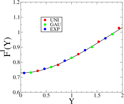
The scaling function FI(Y)superscript𝐹I𝑌F^{\rm I}(Y) is even. Its behavior at small Y𝑌Y reads

FI(Y)=f0+f2Y2+,superscript𝐹I𝑌subscript𝑓0subscript𝑓2superscript𝑌2F^{\rm I}(Y)=f_{0}+f_{2}Y^{2}+\cdots, (5.33)

with

f0subscript𝑓0\displaystyle f_{0} =\displaystyle= Ai(0)Ai(0)=31/3Γ(2/3)Γ(1/3)=0.729011,superscriptAi0Ai0superscript313Γ23Γ130.729011\displaystyle-\frac{{\mathop{\rm Ai}}^{\prime}(0)}{{\mathop{\rm Ai}}(0)}=\frac{3^{1/3}\Gamma(2/3)}{\Gamma(1/3)}=0.729011,
f2subscript𝑓2\displaystyle f_{2} =\displaystyle= 12+(Ai(0)Ai(0))3=123(Γ(2/3)Γ(1/3))3=0.112561.12superscriptsuperscriptAi0Ai03123superscriptΓ23Γ1330.112561\displaystyle\frac{1}{2}+\left(\frac{{\mathop{\rm Ai}}^{\prime}(0)}{{\mathop{\rm Ai}}(0)}\right)^{3}=\frac{1}{2}-3\left(\frac{\Gamma(2/3)}{\Gamma(1/3)}\right)^{3}=0.112561. (5.34)

Its behavior at large Y𝑌Y,

FI(Y)(|Y|2)1/2,superscript𝐹I𝑌superscript𝑌212F^{\rm I}(Y)\approx\left(\frac{|Y|}{2}\right)^{1/2}, (5.35)

yields the estimate

γ(πg1(0)|E|w2)1/2,𝛾superscript𝜋subscript𝑔10𝐸𝑤212\gamma\approx\left(\frac{\pi g_{1}(0)|E|w}{2}\right)^{1/2}, (5.36)

in agreement with the small-x𝑥x behavior in Regime II (see (5.45)).

The scaling function FI(Y)superscript𝐹I𝑌F^{\rm I}(Y) entering the prediction (5.31) is plotted in figure 6. A good agreement is observed with numerical results for the Lyapunov exponent (symbols), based on products of 109superscript10910^{9} matrices for uniform, Gaussian and exponential disorders with w=0.0025𝑤0.0025w=0.0025. The corresponding values of g1(0)subscript𝑔10g_{1}(0) are given in table 2.

Refer to caption
Figure 6: The universal scaling function FI(Y)superscript𝐹I𝑌F^{\rm I}(Y) entering the prediction (5.31) for the Lyapunov exponent of the diamond chain in Regime I, against the rescaled energy variable Y𝑌Y. Symbols: Numerical results for three disorder distributions: uniform, Gaussian and exponential, with w=0.0025𝑤0.0025w=0.0025.

Regime II (Ewsimilar-to𝐸𝑤E\sim w).

This second regime is parametrized by the scaling variable

x=Ew.𝑥𝐸𝑤x=\frac{E}{w}. (5.37)

The heuristic reasoning predicts that typical Riccati variables are of order unity. As a consequence, no rescaling of the variable p𝑝p is involved in the analysis of (5.18). Keeping only terms proportional to w𝑤w, the latter equation boils down to

(p2μ(x)2)L(p)+2pL(p)=1,superscript𝑝2𝜇superscript𝑥2superscript𝐿𝑝2𝑝𝐿𝑝1(p^{2}-\mu(x)^{2})L^{\prime}(p)+2pL(p)=1, (5.38)

where we have introduced the complex function

μ(x)=α(x)iβ(x)=(h1(x)iπg1(x)x)1/2,𝜇𝑥𝛼𝑥i𝛽𝑥superscriptsubscript1𝑥i𝜋subscript𝑔1𝑥𝑥12\mu(x)=\alpha(x)-{\rm i}\beta(x)=\left(\frac{h_{1}(x)-{\rm i}\pi g_{1}(x)}{x}\right)^{1/2}, (5.39)

hence

α(x)=1|x|2(|x|h1(x)2+π2g1(x)2+xh1(x))1/2,𝛼𝑥1𝑥2superscript𝑥subscript1superscript𝑥2superscript𝜋2subscript𝑔1superscript𝑥2𝑥subscript1𝑥12\displaystyle\alpha(x)=\frac{1}{|x|\sqrt{2}}\left(|x|\sqrt{h_{1}(x)^{2}+\pi^{2}g_{1}(x)^{2}}+xh_{1}(x)\right)^{1/2},
β(x)=1x2(|x|h1(x)2+π2g1(x)2xh1(x))1/2.𝛽𝑥1𝑥2superscript𝑥subscript1superscript𝑥2superscript𝜋2subscript𝑔1superscript𝑥2𝑥subscript1𝑥12\displaystyle\beta(x)=\frac{1}{x\sqrt{2}}\left(|x|\sqrt{h_{1}(x)^{2}+\pi^{2}g_{1}(x)^{2}}-xh_{1}(x)\right)^{1/2}. (5.40)

We recall that g1(x)subscript𝑔1𝑥g_{1}(x) is even and h1(x)subscript1𝑥h_{1}(x) is odd, and so α(x)𝛼𝑥\alpha(x) is even and β(x)𝛽𝑥\beta(x) is odd. The solution to (5.38) is

L(p)=1p+μ(x).𝐿𝑝1𝑝𝜇𝑥L(p)=\frac{1}{p+\mu(x)}. (5.41)

There can indeed be no pole at p=μ(x)𝑝𝜇𝑥p=\mu(x), whose real part α(x)𝛼𝑥\alpha(x) is positive. The corresponding invariant distribution of the Riccati variable is Cauchy:

f(R)=α(x)π((R+β(x))2+α(x)2).𝑓𝑅𝛼𝑥𝜋superscript𝑅𝛽𝑥2𝛼superscript𝑥2f(R)=\frac{\alpha(x)}{\pi\left((R+\beta(x))^{2}+\alpha(x)^{2}\right)}. (5.42)

The scaling behavior of the Lyapunov exponent is obtained by linearizing the expression (5.14). We thus obtain γηCR𝛾delimited-⟨⟩superscript𝜂𝐶delimited-⟨⟩𝑅\gamma\approx-\langle\eta^{C}\rangle\langle R\rangle, with ηC=E=xwdelimited-⟨⟩superscript𝜂𝐶𝐸𝑥𝑤\langle\eta^{C}\rangle=E=xw and R=β(x)delimited-⟨⟩𝑅𝛽𝑥\langle R\rangle=-\beta(x), by symmetry, and so

γwFII(x),𝛾𝑤superscript𝐹II𝑥\gamma\approx w\,F^{\rm II}(x), (5.43)

in qualitative agreement with the heuristic reasoning. The corresponding scaling function,

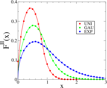
FII(x)=xβ(x)=12(|x|h1(x)2+π2g1(x)2xh1(x))1/2,superscript𝐹II𝑥𝑥𝛽𝑥12superscript𝑥subscript1superscript𝑥2superscript𝜋2subscript𝑔1superscript𝑥2𝑥subscript1𝑥12F^{\rm II}(x)=x\beta(x)=\frac{1}{\sqrt{2}}\left(|x|\sqrt{h_{1}(x)^{2}+\pi^{2}g_{1}(x)^{2}}-xh_{1}(x)\right)^{1/2}, (5.44)

is non-universal, as it depends on the full shape of the disorder distribution, through the functions g1(x)subscript𝑔1𝑥g_{1}(x) and h1(x)subscript1𝑥h_{1}(x), investigated in B.2.

The function FII(x)superscript𝐹II𝑥F^{\rm II}(x) is even, as should be. For small values of x𝑥x, we have

FII(x)(πg1(0)|x|2)1/2,superscript𝐹II𝑥superscript𝜋subscript𝑔10𝑥212F^{\rm II}(x)\approx\left(\frac{\pi g_{1}(0)|x|}{2}\right)^{1/2}, (5.45)

so that a smooth crossover to Regime I is observed (see (5.36)).

For the uniform, Gaussian and exponential distributions, explicit expressions of g1(x)subscript𝑔1𝑥g_{1}(x) are given in B.3, whereas h1(x)subscript1𝑥h_{1}(x) is expressed as an integral that can be carried out in closed form only for Gaussian disorder. The resulting scaling functions FII(x)superscript𝐹II𝑥F^{\rm II}(x) are plotted in figure 7. The prediction (5.43) is found in excellent agreement with numerical results for the Lyapunov exponent (symbols), based on products of 108superscript10810^{8} matrices for each type disorder, with w=0.0025𝑤0.0025w=0.0025. For the uniform distribution, g1(x)subscript𝑔1𝑥g_{1}(x) vanishes identically for |x|>3𝑥3|x|>\sqrt{3} (see (2.23)). As a consequence, FII(x)superscript𝐹II𝑥F^{\rm II}(x) also vanishes there, implying that γ𝛾\gamma falls off more rapidly than linearly in w𝑤w in that range.

Refer to caption
Figure 7: The non-universal scaling functions FII(x)superscript𝐹II𝑥F^{\rm II}(x) entering the prediction (5.43) for the Lyapunov exponent of the diamond chain in Regime II, against the rescaled energy variable x𝑥x, for three disorder distributions: uniform, Gaussian and exponential. Symbols: numerical results for w=0.0025𝑤0.0025w=0.0025.

Gathering our findings on both scaling regimes at weak disorder, we predict that the Lyapunov exponent is a highly non-monotonic function of energy. Considering only positive energies for definiteness, γ𝛾\gamma exhibits a minimum at the center of the dispersive band (E=0𝐸0E=0), scaling as w4/3superscript𝑤43w^{4/3} (Regime I), a maximum for Ewsimilar-to𝐸𝑤E\sim w, scaling as w𝑤w (Regime II), a second minimum near the middle of the dispersive band, scaling as w2superscript𝑤2w^{2}, before it reaches values of order unity if E𝐸E exceeds the outer band edge (E>22𝐸22E>2\sqrt{2}) and then keeps growing indefinitely. The highly non-monotonic profile sketched above is a weak-disorder feature, which only takes place below some non-universal threshold. The minimum at the band center only occurs below wc0.32subscript𝑤𝑐0.32w_{c}\approx 0.32 for the uniform distribution, and below wc0.90subscript𝑤𝑐0.90w_{c}\approx 0.90 for the Gaussian distribution, with the conventions used in this work. This explains why it is not visible on the data shown in Reference [12]. For the exponential distribution, the maximum for Ewsimilar-to𝐸𝑤E\sim w disappears at wc1.69subscript𝑤𝑐1.69w_{c}\approx 1.69, and so the Lyapunov exponent increases monotonically with energy whenever w𝑤w is above wcsubscript𝑤𝑐w_{c}.

6 Discussion

We have investigated the scaling behavior of the localization length in the weak-disorder regime of various 1D structures having flat bands. The foremost feature is the power-law divergence ξwνsimilar-to𝜉superscript𝑤𝜈\xi\sim w^{-\nu} of the localization length at weak disorder. Earlier studies [12, 13, 14, 15, 16] have shown that the two well-known values of the exponent ν𝜈\nu pertaining to the Anderson problem on the chain,

ν=2/3,2,𝜈232\nu=2/3,\quad 2, (6.1)

are supplemented by a few more more exotic values

ν=0,1/2,1,4/3,𝜈012143\nu=0,\quad 1/2,\quad 1,\quad 4/3, (6.2)

pertaining to 1D flat-band systems. To our knowledge, whether the above list is complete or whether it can be derived by systematic reasoning are still open questions.

The main focus of the present work has been on the full scaling functions describing the dependence of the Lyapunov exponent (inverse localization length) γ𝛾\gamma on energy E𝐸E and disorder width w𝑤w throughout weakly disordered flat bands. A careful distinction has been made between situations where the scaling functions are universal (i.e., depend on the disorder distribution only through its width) and where they depend on the shape of the disorder distribution. Three examples (stub chain, pyrochlore ladder, diamond chain), exhausting the full list (6.2) of exotic exponents known to date, have been analyzed in detail. In each case, the analysis of the localization length at weak disorder has been reduced to investigating the Lyapunov exponent of products of random 2×2222\times 2 transfer matrices. The latter reduction, which is asymptotically exact to leading order in the weak-disorder regime, can be thought of as a thorough implementation of the detangling procedure put forward in Reference [13].

Our main specific findings are as follows. On the stub chain (section 3), where one central flat band is isolated from two lateral dispersive ones, the localization length remains microscopic at weak disorder. Its behavior is only accessible by perturbative and numerical means. Its non-universal dependence on the ratio x=E/w𝑥𝐸𝑤x=E/w exhibits several features of interest (see figure 2 and table 1). In particular, the Lyapunov exponent takes a constant value γsubscript𝛾\gamma_{\infty} (see (3.12)) for |x|1much-greater-than𝑥1|x|\gg 1, i.e., w|E|1much-less-than𝑤𝐸much-less-than1w\ll|E|\ll 1. The latter constant is dictated by the band structure of the pristine system. It is formally infinite in situations where all bands are flat. An interesting example is provided by the diamond ladder subjected to a magnetic field, in the case where each unit cell is pierced by half a flux quantum [38, 39]. The spectrum of that system consists of three flat bands at energies E=0𝐸0E=0, ±2plus-or-minus2\pm 2. There, omitting details, we predict a logarithmic divergence of the Lyapunov exponent of the form γln|x|+K𝛾𝑥𝐾\gamma\approx\ln|x|+K for |x|1much-greater-than𝑥1|x|\gg 1, where K𝐾K is an explicit non-universal constant, depending on the full shape of the disorder distribution.

In the other geometries considered here, the flat bands are not isolated from the dispersive ones, and so the localization length diverges in the weak-disorder regime. On the pyrochlore ladder (section 4), the two flat bands are tangent to a dispersive one. The localization length has scaling exponent 1/2 and obeys the non-universal scaling law (4.22). The dependence of the scaling function F(pyro)(x)superscript𝐹pyro𝑥F^{\rm(pyro)}(x) on the disorder distribution is given by (4.23) in terms of the functions g2(x)subscript𝑔2𝑥g_{2}(x) and h2(x)subscript2𝑥h_{2}(x), investigated in B.2 and characteristic of the Cauchy effective disorder. On the diamond chain (section 5), a central flat band intersects two symmetric dispersive ones. The situation at weak disorder is richer than the previous cases. The localization length now exhibits two successive scaling regimes. In Regime I (Ew5/3similar-to𝐸superscript𝑤53E\sim w^{5/3}), it diverges with exponent 4/3, according to (5.31), and a universal scaling function FI(Y)superscript𝐹I𝑌F^{\rm I}(Y) given by (5.32). In Regime II (Ewsimilar-to𝐸𝑤E\sim w), it diverges with exponent 1, according to (5.43), and a non-universal scaling function FII(x)superscript𝐹II𝑥F^{\rm II}(x) (see (5.44)) depending on the full shape of the disorder distribution, through the functions g1(x)subscript𝑔1𝑥g_{1}(x) and h1(x)subscript1𝑥h_{1}(x) investigated in B.1. Here, too, the lack of universality in this second regime originates in the occurrence of a broad probability distribution of the effective disorder, exhibiting symmetric Cauchy tails.

It is a pleasure to thank Alexei Andreanov, Sergej Flach and Julien Vidal for useful correspondence.

Appendix A Cauchy tails

Cauchy tails in probability distributions play a central part in the analysis of the pyrochlore ladder (section 4) and the diamond chain (section 5).

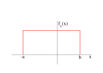
Let us introduce this notion on a simple and explicit example. Consider a random variable x𝑥x with a uniform distribution on an interval containing 0, i.e.,

fx(x)=1a+b(a<x<b).subscript𝑓𝑥𝑥1𝑎𝑏𝑎𝑥𝑏f_{x}(x)=\frac{1}{a+b}\qquad(-a<x<b). (1.1)

Its reciprocal y=1/x𝑦1𝑥y=1/x has the probability distribution

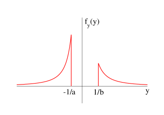
fy(y)=1(a+b)y2(y<1/a&y>1/b).subscript𝑓𝑦𝑦1𝑎𝑏superscript𝑦2formulae-sequence𝑦1𝑎𝑦1𝑏f_{y}(y)=\frac{1}{(a+b)y^{2}}\qquad(y<-1/a\ \ \&\ \ y>1/b). (1.2)

These distributions are sketched in figure 8.
Refer to caption
Refer to caption
Figure 8: Sketchy plot of the probability distributions fx(x)subscript𝑓𝑥𝑥f_{x}(x) and fy(y)subscript𝑓𝑦𝑦f_{y}(y) given by (1.1) and (1.2), for a:b=3:2:𝑎𝑏3:2a:b=3:2.

The occurrence of symmetric Cauchy tails falling off as 1/y21superscript𝑦21/y^{2} as y±𝑦plus-or-minusy\to\pm\infty is a generic feature of the distribution of a variable y𝑦y equal to the reciprocal of a variable x𝑥x which may vanish. The strength G𝐺G of these Cauchy tails, or the Cauchy strength of the variable y𝑦y for short, is defined as

G=limy±y2fy(y)=δ(1y).𝐺subscript𝑦plus-or-minussuperscript𝑦2subscript𝑓𝑦𝑦delimited-⟨⟩𝛿1𝑦G=\lim_{y\to\pm\infty}y^{2}f_{y}(y)=\left\langle\delta\left(\frac{1}{y}\right)\right\rangle. (1.3)

In the above example, this reads

G=δ(x)=fx(0)=1a+b,𝐺delimited-⟨⟩𝛿𝑥subscript𝑓𝑥01𝑎𝑏G=\langle\delta(x)\rangle=f_{x}(0)=\frac{1}{a+b}, (1.4)

in agreement with (1.2).

Consider for definiteness the regime where a𝑎a and b𝑏b are simultaneously large. There, x𝑥x is typically large, and so y𝑦y is typically small. There are however rare circumstances where x𝑥x is close to zero, and so y𝑦y is much larger than its typical value. The Cauchy strength G𝐺G, introduced above, characterizes atypical large values of y𝑦y, whereas its typical small values are characterized by its symmetric mean value, i.e.,

H=y=limΛΛΛyfy(y)dy.𝐻delimited-⟨⟩𝑦subscriptΛsuperscriptsubscriptΛΛ𝑦subscript𝑓𝑦𝑦differential-d𝑦H=\langle y\rangle=\lim_{\Lambda\to\infty}\int_{-\Lambda}^{\Lambda}y\,f_{y}(y)\,{\rm d}y. (1.5)

In the above example, we have

H=1x=fx(x)dxx=limε0(ε+ε)fx(x)dxx,𝐻delimited-⟨⟩1𝑥superscriptsubscriptsubscript𝑓𝑥𝑥d𝑥𝑥subscript𝜀0superscriptsubscript𝜀superscriptsubscript𝜀subscript𝑓𝑥𝑥d𝑥𝑥H=\left\langle\frac{1}{x}\right\rangle=\mathchoice{{\vbox{\hbox{$\textstyle-$}}\kern-4.86108pt}}{{\vbox{\hbox{$\scriptstyle-$}}\kern-3.25pt}}{{\vbox{\hbox{$\scriptscriptstyle-$}}\kern-2.29166pt}}{{\vbox{\hbox{$\scriptscriptstyle-$}}\kern-1.875pt}}\!\int_{-\infty}^{\infty}\frac{f_{x}(x)\,{\rm d}x}{x}=\lim_{\varepsilon\to 0}\left(\int_{-\infty}^{-\varepsilon}+\int_{\varepsilon}^{\infty}\right)\frac{f_{x}(x)\,{\rm d}x}{x}, (1.6)

where the bar denotes the Cauchy principal value, i.e., explicitly,

H=limε0(aε+εb)dx(a+b)x=1a+blnba.𝐻subscript𝜀0superscriptsubscript𝑎𝜀superscriptsubscript𝜀𝑏d𝑥𝑎𝑏𝑥1𝑎𝑏𝑏𝑎H=\lim_{\varepsilon\to 0}\left(\int_{-a}^{-\varepsilon}+\int_{\varepsilon}^{b}\right)\frac{{\rm d}x}{(a+b)x}=\frac{1}{a+b}\ln\frac{b}{a}. (1.7)

This expression vanishes in the symmetric situation where a=b𝑎𝑏a=b, as should be.

In spite of their interpretation, the Cauchy strength G𝐺G and the mean value H𝐻H of y𝑦y have the same dimension. As a consequence, they are of the same order of magnitude in the weak-disorder regime where a𝑎a and b𝑏b are simultaneously large.

Appendix B Effective disorder on the diamond chain and on the pyrochlore ladder

This appendix is devoted to an investigation of the effective disorder on the diamond chain and the pyrochlore ladder. We consider a symmetric continuous distribution ρ(v)𝜌𝑣\rho(v) of the random potentials, such that all moments are finite. The disorder width w𝑤w is defined by setting v2=w2delimited-⟨⟩superscript𝑣2superscript𝑤2\langle v^{2}\rangle=w^{2}. The kurtosis is defined by

κ=v4v22=v4w4.𝜅delimited-⟨⟩superscript𝑣4superscriptdelimited-⟨⟩superscript𝑣22delimited-⟨⟩superscript𝑣4superscript𝑤4\kappa=\frac{\langle v^{4}\rangle}{\langle v^{2}\rangle^{2}}=\frac{\langle v^{4}\rangle}{w^{4}}. (2.1)

The Fourier transform of the distribution reads

ρ^(q)=iqv=iqvρ(v)dv.^𝜌𝑞delimited-⟨⟩superscripti𝑞𝑣superscriptsubscriptsuperscripti𝑞𝑣𝜌𝑣differential-d𝑣{\widehat{\rho}}(q)=\langle\rme^{{\rm i}qv}\rangle=\int_{-\infty}^{\infty}\rme^{{\rm i}qv}\rho(v){\rm d}v. (2.2)

B.1 The effective disorder on the diamond chain

The effective disorder on the diamond chain is characterized by its Cauchy strength and its mean value (see (5.10)):

G1(E)=δ(ηA+ηBηAηB),H1(E)=ηAηBηA+ηB,formulae-sequencesubscript𝐺1𝐸delimited-⟨⟩𝛿superscript𝜂𝐴superscript𝜂𝐵superscript𝜂𝐴superscript𝜂𝐵subscript𝐻1𝐸delimited-⟨⟩superscript𝜂𝐴superscript𝜂𝐵superscript𝜂𝐴superscript𝜂𝐵G_{1}(E)=\left\langle\delta\left(\frac{\eta^{A}+\eta^{B}}{\eta^{A}\eta^{B}}\right)\right\rangle,\qquad H_{1}(E)=\left\langle\frac{\eta^{A}\eta^{B}}{\eta^{A}+\eta^{B}}\right\rangle, (2.3)

with

ηA=EvA,ηB=EvB.formulae-sequencesuperscript𝜂𝐴𝐸superscript𝑣𝐴superscript𝜂𝐵𝐸superscript𝑣𝐵\eta^{A}=E-v^{A},\qquad\eta^{B}=E-v^{B}. (2.4)

The Cauchy strength can be evaluated as

G1(E)subscript𝐺1𝐸\displaystyle G_{1}(E) =\displaystyle= ρ(EηA)dηAρ(EηB)dηBδ(ηA+ηBηAηB)superscriptsubscript𝜌𝐸superscript𝜂𝐴differential-dsuperscript𝜂𝐴superscriptsubscript𝜌𝐸superscript𝜂𝐵differential-dsuperscript𝜂𝐵𝛿superscript𝜂𝐴superscript𝜂𝐵superscript𝜂𝐴superscript𝜂𝐵\displaystyle\int_{-\infty}^{\infty}\rho(E-\eta^{A}){\rm d}\eta^{A}\int_{-\infty}^{\infty}\rho(E-\eta^{B}){\rm d}\eta^{B}\delta\left(\frac{\eta^{A}+\eta^{B}}{\eta^{A}\eta^{B}}\right) (2.5)
=\displaystyle= ρ(Eη)ρ(E+η)η2dη.superscriptsubscript𝜌𝐸𝜂𝜌𝐸𝜂superscript𝜂2differential-d𝜂\displaystyle\int_{-\infty}^{\infty}\rho(E-\eta)\rho(E+\eta)\eta^{2}{\rm d}\eta.

The second line is obtained by integrating over ηBsuperscript𝜂𝐵\eta^{B}, denoting ηAsuperscript𝜂𝐴\eta^{A} as η𝜂\eta. This can be recast in Fourier space as

G1(E)=12πρ^(q)iqEd2dq2(ρ^(q)iqE)dq.subscript𝐺1𝐸12𝜋superscriptsubscript^𝜌𝑞superscripti𝑞𝐸superscriptd2dsuperscript𝑞2^𝜌𝑞superscripti𝑞𝐸differential-d𝑞G_{1}(E)=-\frac{1}{2\pi}\int_{-\infty}^{\infty}{\widehat{\rho}}(q)\rme^{{\rm i}qE}\frac{{\rm d}^{2}}{{\rm d}q^{2}}\left({\widehat{\rho}}(q)\rme^{{\rm i}qE}\right){\rm d}q. (2.6)

The latter expression is more amenable to an explicit evaluation for specific disorder distributions.

The mean value can be evaluated as

H1(E)=(EvA)(EvB)2EvAvB=E214(vAvB)22EvAvB.subscript𝐻1𝐸delimited-⟨⟩𝐸superscript𝑣𝐴𝐸superscript𝑣𝐵2𝐸superscript𝑣𝐴superscript𝑣𝐵𝐸214delimited-⟨⟩superscriptsuperscript𝑣𝐴superscript𝑣𝐵22𝐸superscript𝑣𝐴superscript𝑣𝐵H_{1}(E)=\left\langle\frac{(E-v^{A})(E-v^{B})}{2E-v^{A}-v^{B}}\right\rangle=\frac{E}{2}-\frac{1}{4}\left\langle\frac{(v^{A}-v^{B})^{2}}{2E-v^{A}-v^{B}}\right\rangle. (2.7)

At this stage it is advantageous to add an infinitesimal imaginary part to E𝐸E. We have

ImH1(E+i0)Imsubscript𝐻1𝐸i0\displaystyle\mathop{\rm Im}\,H_{1}(E+{\rm i}0) =\displaystyle= π4(vAvB)2δ(2EvAvB)𝜋4delimited-⟨⟩superscriptsuperscript𝑣𝐴superscript𝑣𝐵2𝛿2𝐸superscript𝑣𝐴superscript𝑣𝐵\displaystyle\frac{\pi}{4}\left\langle(v^{A}-v^{B})^{2}\delta(2E-v^{A}-v^{B})\right\rangle (2.8)
=\displaystyle= π4ρ(vA)dvAρ(vB)dvB(vAvB)2𝜋4superscriptsubscript𝜌superscript𝑣𝐴differential-dsuperscript𝑣𝐴superscriptsubscript𝜌superscript𝑣𝐵differential-dsuperscript𝑣𝐵superscriptsuperscript𝑣𝐴superscript𝑣𝐵2\displaystyle\frac{\pi}{4}\int_{-\infty}^{\infty}\rho(v^{A}){\rm d}v^{A}\int_{-\infty}^{\infty}\rho(v^{B}){\rm d}v^{B}(v^{A}-v^{B})^{2}
×\displaystyle\times δ(2EvAvB).𝛿2𝐸superscript𝑣𝐴superscript𝑣𝐵\displaystyle\delta(2E-v^{A}-v^{B}).

Setting vA=Eηsuperscript𝑣𝐴𝐸𝜂v^{A}=E-\eta, vB=E+ηsuperscript𝑣𝐵𝐸𝜂v^{B}=E+\eta, we get

ImH1(E+i0)=πρ(Eη)ρ(E+η)η2dη=πG1(E).Imsubscript𝐻1𝐸i0𝜋superscriptsubscript𝜌𝐸𝜂𝜌𝐸𝜂superscript𝜂2differential-d𝜂𝜋subscript𝐺1𝐸\mathop{\rm Im}\,H_{1}(E+{\rm i}0)=\pi\int_{-\infty}^{\infty}\rho(E-\eta)\rho(E+\eta)\eta^{2}{\rm d}\eta=\pi G_{1}(E). (2.9)

The real part H1(E)ReH1(E+i0)subscript𝐻1𝐸Resubscript𝐻1𝐸i0H_{1}(E)\equiv\mathop{\rm Re}\,H_{1}(E+{\rm i}0) can be reconstructed from the imaginary part by an integral equation somehow similar to the Kramers-Kronig dispersion relations:

H1(E)=E2+G1(E)dEEE,H_{1}(E)=\frac{E}{2}+\mathchoice{{\vbox{\hbox{$\textstyle-$}}\kern-4.86108pt}}{{\vbox{\hbox{$\scriptstyle-$}}\kern-3.25pt}}{{\vbox{\hbox{$\scriptscriptstyle-$}}\kern-2.29166pt}}{{\vbox{\hbox{$\scriptscriptstyle-$}}\kern-1.875pt}}\!\int_{-\infty}^{\infty}\frac{G_{1}(E^{\prime}){\rm d}E^{\prime}}{E^{\prime}-E}, (2.10)

where the bar again denotes the Cauchy principal value.

The scaling dependence of G1(E)subscript𝐺1𝐸G_{1}(E) and H1(E)subscript𝐻1𝐸H_{1}(E) on w𝑤w reads

G1(E)=wg1(x),H1(E)=wh1(x),x=Ew.formulae-sequencesubscript𝐺1𝐸𝑤subscript𝑔1𝑥formulae-sequencesubscript𝐻1𝐸𝑤subscript1𝑥𝑥𝐸𝑤G_{1}(E)=wg_{1}(x),\qquad H_{1}(E)=wh_{1}(x),\qquad x=\frac{E}{w}. (2.11)

The functions G1(E)subscript𝐺1𝐸G_{1}(E) and g1(x)subscript𝑔1𝑥g_{1}(x) are even, whereas H1(E)subscript𝐻1𝐸H_{1}(E) and h1(x)subscript1𝑥h_{1}(x) are odd, and (2.10) translates to

h1(x)=x2+g1(x)dxxx.h_{1}(x)=\frac{x}{2}+\mathchoice{{\vbox{\hbox{$\textstyle-$}}\kern-4.86108pt}}{{\vbox{\hbox{$\scriptstyle-$}}\kern-3.25pt}}{{\vbox{\hbox{$\scriptscriptstyle-$}}\kern-2.29166pt}}{{\vbox{\hbox{$\scriptscriptstyle-$}}\kern-1.875pt}}\!\int_{-\infty}^{\infty}\frac{g_{1}(x^{\prime}){\rm d}x^{\prime}}{x^{\prime}-x}. (2.12)

B.2 The effective disorder on the pyrochlore ladder

The effective disorder on the pyrochlore ladder is characterized by its Cauchy strength and its mean value (see (4.19)):

G2(E)=δ(η(1)+η(2)η(1)η(2)),H2(E)=η(1)η(2)η(1)+η(2),formulae-sequencesubscript𝐺2𝐸delimited-⟨⟩𝛿superscript𝜂1superscript𝜂2superscript𝜂1superscript𝜂2subscript𝐻2𝐸delimited-⟨⟩superscript𝜂1superscript𝜂2superscript𝜂1superscript𝜂2G_{2}(E)=\left\langle\delta\left(\frac{\eta^{(1)}+\eta^{(2)}}{\eta^{(1)}\eta^{(2)}}\right)\right\rangle,\qquad H_{2}(E)=\left\langle\frac{\eta^{(1)}\eta^{(2)}}{\eta^{(1)}+\eta^{(2)}}\right\rangle, (2.13)

with

η(1)=2EvAvC,η(2)=2EvBvD.formulae-sequencesuperscript𝜂12𝐸superscript𝑣𝐴superscript𝑣𝐶superscript𝜂22𝐸superscript𝑣𝐵superscript𝑣𝐷\eta^{(1)}=2E-v^{A}-v^{C},\qquad\eta^{(2)}=2E-v^{B}-v^{D}. (2.14)

The expressions (2.13) and (2.14) are similar to (2.3) and (2.4), up to two differences: energy is doubled (E2E𝐸2𝐸E\to 2E), and each random potential is replaced by a sum of two independent potentials (vAvA+vCsuperscript𝑣𝐴superscript𝑣𝐴superscript𝑣𝐶v^{A}\to v^{A}+v^{C}, vBvB+vDsuperscript𝑣𝐵superscript𝑣𝐵superscript𝑣𝐷v^{B}\to v^{B}+v^{D}). The latter operation amounts to replacing the disorder distribution ρ𝜌\rho by ρ2=ρρsubscript𝜌2𝜌𝜌\rho_{2}=\rho*\rho, i.e.,

ρ2(v)=ρ(u)ρ(vu)du,subscript𝜌2𝑣superscriptsubscript𝜌𝑢𝜌𝑣𝑢differential-d𝑢\rho_{2}(v)=\int_{-\infty}^{\infty}\rho(u)\rho(v-u){\rm d}u, (2.15)

whose Fourier transform is ρ^2(q)=ρ^(q)2subscript^𝜌2𝑞^𝜌superscript𝑞2{\widehat{\rho}}_{2}(q)={\widehat{\rho}}(q)^{2}. Applying these changes to the results (2.5), (2.6) and (2.10), we readily obtain

G2(E)subscript𝐺2𝐸\displaystyle G_{2}(E) =\displaystyle= ρ2(2Eη)ρ2(2E+η)η2dηsuperscriptsubscriptsubscript𝜌22𝐸𝜂subscript𝜌22𝐸𝜂superscript𝜂2differential-d𝜂\displaystyle\int_{-\infty}^{\infty}\rho_{2}(2E-\eta)\rho_{2}(2E+\eta)\eta^{2}{\rm d}\eta (2.16)
=\displaystyle= 12πρ^(q)22iqEd2dq2(ρ^(q)22iqE)dq12𝜋superscriptsubscript^𝜌superscript𝑞2superscript2i𝑞𝐸superscriptd2dsuperscript𝑞2^𝜌superscript𝑞2superscript2i𝑞𝐸differential-d𝑞\displaystyle-\frac{1}{2\pi}\int_{-\infty}^{\infty}{\widehat{\rho}}(q)^{2}\rme^{2{\rm i}qE}\frac{{\rm d}^{2}}{{\rm d}q^{2}}\left({\widehat{\rho}}(q)^{2}\rme^{2{\rm i}qE}\right){\rm d}q

and

H2(E)=E+G2(E)dEEE.H_{2}(E)=E+\mathchoice{{\vbox{\hbox{$\textstyle-$}}\kern-4.86108pt}}{{\vbox{\hbox{$\scriptstyle-$}}\kern-3.25pt}}{{\vbox{\hbox{$\scriptscriptstyle-$}}\kern-2.29166pt}}{{\vbox{\hbox{$\scriptscriptstyle-$}}\kern-1.875pt}}\!\int_{-\infty}^{\infty}\frac{G_{2}(E^{\prime}){\rm d}E^{\prime}}{E^{\prime}-E}. (2.17)

The scaling dependence of G2(E)subscript𝐺2𝐸G_{2}(E) and H2(E)subscript𝐻2𝐸H_{2}(E) on w𝑤w reads

G2(E)=wg2(x),H2(E)=wh2(x),x=Ew.formulae-sequencesubscript𝐺2𝐸𝑤subscript𝑔2𝑥formulae-sequencesubscript𝐻2𝐸𝑤subscript2𝑥𝑥𝐸𝑤G_{2}(E)=wg_{2}(x),\qquad H_{2}(E)=wh_{2}(x),\qquad x=\frac{E}{w}. (2.18)

The functions G2(E)subscript𝐺2𝐸G_{2}(E) and g2(x)subscript𝑔2𝑥g_{2}(x) are even, whereas H2(E)subscript𝐻2𝐸H_{2}(E) and h2(x)subscript2𝑥h_{2}(x) are odd, and (2.17) translates to

h2(x)=x+g2(x)dxxx.h_{2}(x)=x+\mathchoice{{\vbox{\hbox{$\textstyle-$}}\kern-4.86108pt}}{{\vbox{\hbox{$\scriptstyle-$}}\kern-3.25pt}}{{\vbox{\hbox{$\scriptscriptstyle-$}}\kern-2.29166pt}}{{\vbox{\hbox{$\scriptscriptstyle-$}}\kern-1.875pt}}\!\int_{-\infty}^{\infty}\frac{g_{2}(x^{\prime}){\rm d}x^{\prime}}{x^{\prime}-x}. (2.19)

B.3 Explicit formulas for specific disorder distributions

In the body of this work we use the following results for three disorder distributions: uniform, Gaussian and exponential.

The uniform distribution.

It reads

ρ(v)=12V(V<v<V).𝜌𝑣12𝑉𝑉𝑣𝑉\rho(v)=\frac{1}{2V}\qquad(-V<v<V). (2.20)

We have v2=V2/3delimited-⟨⟩superscript𝑣2superscript𝑉23\langle v^{2}\rangle=V^{2}/3 and v4=V2/5delimited-⟨⟩superscript𝑣4superscript𝑉25\langle v^{4}\rangle=V^{2}/5, and so

w=V3,κ=95.formulae-sequence𝑤𝑉3𝜅95w=\frac{V}{\sqrt{3}},\qquad\kappa=\frac{9}{5}. (2.21)

Its Fourier transform reads

ρ^(q)=sinqVqV.^𝜌𝑞𝑞𝑉𝑞𝑉{\widehat{\rho}}(q)=\frac{\sin qV}{qV}. (2.22)

Inserting the latter expression into (2.6) and (2.16), we obtain the following expressions for g1(x)subscript𝑔1𝑥g_{1}(x) and g2(x)subscript𝑔2𝑥g_{2}(x) for x0𝑥0x\geq 0 (these functions are even):

g1(x)={118(3x)3(0<x<3),0(x>3),g_{1}(x)=\left\{\matrix{{\displaystyle{1\over 18}}(\sqrt{3}-x)^{3}\hfill&(0<x<\sqrt{3}),\hfill\cr\cr 0\hfill&(x>\sqrt{3}),\hfill}\right. (2.23)
g2(x)={g(x)(0<x<3/2),8135(3x)5(3/2<x<3),0(x>3),g_{2}(x)=\left\{\matrix{g_{\star}(x)\hfill&\left(0<x<\sqrt{3}/2\right),\hfill\cr\cr{\displaystyle{8\over 135}}(\sqrt{3}-x)^{5}\hfill&\left(\sqrt{3}/2<x<\sqrt{3}\right),\hfill\cr\cr 0\hfill&\;(x>\sqrt{3}),\hfill}\right. (2.24)

with

g(x)=2315439x2+89x38327x4+845x5.subscript𝑔𝑥2315439superscript𝑥289superscript𝑥38327superscript𝑥4845superscript𝑥5g_{\star}(x)=\frac{2\sqrt{3}}{15}-\frac{4\sqrt{3}}{9}x^{2}+\frac{8}{9}x^{3}-\frac{8\sqrt{3}}{27}x^{4}+\frac{8}{45}x^{5}. (2.25)

The vanishing of g1(x)subscript𝑔1𝑥g_{1}(x) and g2(x)subscript𝑔2𝑥g_{2}(x) for |x|>3𝑥3|x|>\sqrt{3}, i.e., |E|>V𝐸𝑉|E|>V, is expected. Indeed in this range none of the η𝜂\eta variables entering (2.4) or (2.14) can vanish. The functions h1(x)subscript1𝑥h_{1}(x) and h2(x)subscript2𝑥h_{2}(x) have not been evaluated in closed form.

The Gaussian distribution.

It reads

ρ(v)=v2/(2w2)w2π.𝜌𝑣superscriptsuperscript𝑣22superscript𝑤2𝑤2𝜋\rho(v)=\frac{\rme^{-v^{2}/(2w^{2})}}{w\sqrt{2\pi}}. (2.26)

We have v2=w2delimited-⟨⟩superscript𝑣2superscript𝑤2\langle v^{2}\rangle=w^{2} and v4=3w4delimited-⟨⟩superscript𝑣43superscript𝑤4\langle v^{4}\rangle=3w^{4}, and so

κ=3.𝜅3\kappa=3. (2.27)

Its Fourier transform reads

ρ^(q)=q2w2/2.^𝜌𝑞superscriptsuperscript𝑞2superscript𝑤22{\widehat{\rho}}(q)=\rme^{-q^{2}w^{2}/2}. (2.28)

Inserting this expression into (2.6) and (2.16), we obtain the simple results

g1(x)=x24π,g2(x)=2x28π.formulae-sequencesubscript𝑔1𝑥superscriptsuperscript𝑥24𝜋subscript𝑔2𝑥superscript2superscript𝑥28𝜋g_{1}(x)=\frac{\rme^{-x^{2}}}{4\sqrt{\pi}},\qquad g_{2}(x)=\frac{\rme^{-2x^{2}}}{\sqrt{8\pi}}. (2.29)

The expressions (2.12) and (2.19) yield

h1(x)subscript1𝑥\displaystyle h_{1}(x) =\displaystyle= x2+iπ4x2erf(ix),𝑥2i𝜋4superscriptsuperscript𝑥2erfi𝑥\displaystyle\frac{x}{2}+\frac{{\rm i}\sqrt{\pi}}{4}\rme^{-x^{2}}{\mathop{\rm erf}}({\rm i}x),
h2(x)subscript2𝑥\displaystyle h_{2}(x) =\displaystyle= x+i2π42x2erf(ix2),𝑥i2𝜋4superscript2superscript𝑥2erfi𝑥2\displaystyle x+\frac{{\rm i}\sqrt{2\pi}}{4}\rme^{-2x^{2}}{\mathop{\rm erf}}({\rm i}x\sqrt{2}), (2.30)

where erferf{\mathop{\rm erf}} is the error function.

The exponential distribution.

The symmetric exponential distribution, also referred to as the Laplace distribution, reads

ρ(v)=|v|/V2V.𝜌𝑣superscript𝑣𝑉2𝑉\rho(v)=\frac{\rme^{-|v|/V}}{2V}. (2.31)

We have v2=2V2delimited-⟨⟩superscript𝑣22superscript𝑉2\langle v^{2}\rangle=2V^{2} and v4=24V4delimited-⟨⟩superscript𝑣424superscript𝑉4\langle v^{4}\rangle=24V^{4}, and so

w=V2,κ=6.formulae-sequence𝑤𝑉2𝜅6w=V\sqrt{2},\qquad\kappa=6. (2.32)

Its Fourier transform reads

ρ^(q)=11+q2V2.^𝜌𝑞11superscript𝑞2superscript𝑉2{\widehat{\rho}}(q)=\frac{1}{1+q^{2}V^{2}}. (2.33)

Inserting the latter expression into (2.6) and (2.16), we obtain the following expressions for g1(x)subscript𝑔1𝑥g_{1}(x) and g2(x)subscript𝑔2𝑥g_{2}(x) for x0𝑥0x\geq 0 (these functions are even):

g1(x)subscript𝑔1𝑥\displaystyle g_{1}(x) =\displaystyle= (216+14x+24x2+13x3)22x,21614𝑥24superscript𝑥213superscript𝑥3superscript22𝑥\displaystyle\left(\frac{\sqrt{2}}{16}+\frac{1}{4}x+\frac{\sqrt{2}}{4}x^{2}+\frac{1}{3}x^{3}\right)\rme^{-2\sqrt{2}x}, (2.34)
g2(x)subscript𝑔2𝑥\displaystyle g_{2}(x) =\displaystyle= (7264+78x+1328x2+113x3+823x4+3215x5)42x.726478𝑥1328superscript𝑥2113superscript𝑥3823superscript𝑥43215superscript𝑥5superscript42𝑥\displaystyle\left(\frac{7\sqrt{2}}{64}+\frac{7}{8}x+\frac{13\sqrt{2}}{8}x^{2}+\frac{11}{3}x^{3}+\frac{8\sqrt{2}}{3}x^{4}+\frac{32}{15}x^{5}\right)\rme^{-4\sqrt{2}x}.

The functions h1(x)subscript1𝑥h_{1}(x) and h2(x)subscript2𝑥h_{2}(x) have not been evaluated in closed form.

To close, we give in table 2 the values of the Cauchy strength of the effective disorder at the center of the flat band at E=0𝐸0E=0 for the two flat-band structures and the three disorder distributions studied in this appendix.

Distribution κ𝜅\kappa g1(0)subscript𝑔10g_{1}(0) g2(0)subscript𝑔20g_{2}(0)
Uniform 95=1.8951.8{\displaystyle{9\over 5}}=1.8 36=0.288675360.288675{\displaystyle{\sqrt{3}\over 6}}=0.288675 2315=0.23094023150.230940{\displaystyle{2\sqrt{3}\over 15}}=0.230940
Gaussian 3 14π=0.14104714𝜋0.141047{\displaystyle{1\over 4\sqrt{\pi}}}=0.141047 18π=0.19947118𝜋0.199471{\displaystyle{1\over\sqrt{8\pi}}}=0.199471
Exponential 6 216=0.0883882160.088388{\displaystyle{\sqrt{2}\over 16}}=0.088388 7264=0.15467972640.154679{\displaystyle{7\sqrt{2}\over 64}}=0.154679
Table 2: Values of the Cauchy strength of the effective disorder at the center of the flat band at E=0𝐸0E=0 for the two flat-band structures studied in this appendix, namely g1(0)subscript𝑔10g_{1}(0) on the diamond chain (see section 5 and B.1) and g2(0)subscript𝑔20g_{2}(0) on the pyrochlore ladder (see section 4 and B.2), and for three disorder distributions, whose kurtosis κ𝜅\kappa is recalled.

References

References

  • [1] Goda M, Nishino S and Matsuda H 2006 Phys. Rev. Lett. 96 126401
  • [2] Nishino S, Matsuda H and Goda M 2007 J. Phys. Soc. Japan 76 024709
  • [3] Chalker J T, Pickles T S and Shukla P 2007 Phys. Rev. B 82 104209
  • [4] Nita M, Ostahie B and Aldea A 2013 Phys. Rev. B 87 125428
  • [5] Shukla P 2018 Phys. Rev. B 98 054206
  • [6] Shukla P 2018 Phys. Rev. B 98 184202
  • [7] Gneiting C, Li Z and Nori F 2018 Phys. Rev. B 98 134203
  • [8] Bilitewski T and Moessner R 2018 Phys. Rev. B 98 235109
  • [9] Abrahams E, Anderson P W, Licciardello D G and Ramakrishnan T V 1979 Phys. Rev. Lett. 42 673
  • [10] Lifshitz I M, Gredeskul S A and Pastur L A 1988 Introduction to the Theory of Disordered Systems (New York: Wiley)
  • [11] Abrahams E (ed) 2010 50 Years of Anderson Localization (Singapore: World Scientific)
  • [12] Leykam D, Flach S, Bahat-Treidel O and Desyatnikov A S 2013 Phys. Rev. B 88 224203
  • [13] Flach S, Leykam D, Bodyfelt J D, Matthies P and Desyatnikov A S 2014 EPL 105 30001
  • [14] Leykam D, Bodyfelt J D, Desyatnikov A S and Flach S 2017 Eur. Phys. J. B 90 1
  • [15] Maimaiti W, Andreanov A, Park H C, Gendelman O and Flach S 2017 Phys. Rev. B 95 115135
  • [16] Ge L 2017 Ann. Phys. (Berlin) 529 1600182
  • [17] Furstenberg H 1963 Trans. Amer. Math. Soc. 108 377
  • [18] Borland R E 1963 Proc. Roy. Soc. A 274 529
  • [19] Carmona R 1982 Duke Math. J. 49 191
  • [20] Pichard J L, Zanon N, Imry Y and Stone A D 1990 J. Phys. (France) 51 587
  • [21] Luck J M 1992 Systèmes désordonnés unidimensionnels (Saclay, France: Collection Aléa)
  • [22] Comtet A, Texier C and Tourigny Y 2013 J. Phys. A 46 254003
  • [23] Thouless D J 1979 Percolation and localization Ill-Condensed Matter ed Balian R, Maynard R and Toulouse G (Amsterdam: North-Holland)
  • [24] Frisch H L and Lloyd S P 1960 Phys. Rev. 120 1175
  • [25] Halperin B I 1965 Phys. Rev. 139 A104
  • [26] Derrida B and Gardner E J 1984 J. Phys. (France) 45 1283
  • [27] Izrailev F M, Ruffo S and Tessieri L 1998 J. Phys. A 31 5263
  • [28] Comtet A, Luck J M, Texier C and Tourigny Y 2013 J. Stat. Phys. 150 13
  • [29] Lloyd P 1969 J. Phys. C 2 1717
  • [30] Dyson F J 1953 Phys. Rev. 92 1331
  • [31] Schmidt H 1957 Phys. Rev. 105 425
  • [32] Klopp F 1999 Duke Math. J. 98 335
  • [33] Klopp F 2002 Commun. Math. Phys. 232 125
  • [34] Nieuwenhuizen T M 1982 Physica A 113 173
  • [35] Nieuwenhuizen T M and Luck J M 1986 J. Phys. A 19 1207
  • [36] Barnes C and Luck J M 1990 J. Phys. A 23 1717
  • [37] Luck J M 1993 J. Stat. Phys. 72 417
  • [38] Vidal J, Douçot B, Mosseri R and Butaud P 2000 Phys. Rev. Lett. 85 3906
  • [39] Douçot B and Vidal J 2002 Phys. Rev. Lett. 88 227005