A model under location uncertainty to predict the mean velocity in wall bounded flows

Abstract

To date no satisfying model exists to explain the mean velocity profile within the whole turbulent layer of canonical wall bounded flows. We propose a modification of the velocity profile expression that ensues from a recently proposed stochastic representation of fluid flows dynamics. This modeling, called modeling under location uncertainty introduces in a rigorous way a subgrid term generalizing the eddy-viscosity assumption and an eddy-induced advection term resulting from turbulence inhomogeneity. This latter term gives rise to a theoretically well-grounded model for the transitional zone between the viscous sublayer and the turbulent sublayer. An expression of the small-scale velocity component is also provided in the viscous zone. Numerical assessment of the results are provided for turbulent boundary layer flows, for pipe flows and channel flows at various Reynolds numbers.

I introduction

The study of mean velocity profiles in wall-bounded flows is generating an intense research effort. Their knowledge is as a matter of fact an immense source of information for many industrial applications and in geophysics to model the interface between atmosphere and ocean. Since the seminal work of Prandtl (1925) and von Karman (1930), the mean velocity profile is known to be linear in a viscous sublayer near the wall and logarithmic within a turbulent sublayer, located before a region of uniform mean profile. These models have been derived from different theoretical arguments and confirmed in a wide variety of experiments (Jiménez and Moser, 2007; Marusic et al., 2010; Klewicki, 2010; Marusic et al., 2013). Between the viscous layer and the logarithmic layer, within an interfacial region, referred to as the buffer zone, no robust model is yet available.

The lack of a model with clear theoretical foundations for the buffer zone is essentially due to a change of the dynamical regime between the viscous and turbulent sublayers. In the former, the molecular friction dominates while in the latter it is a large-scale turbulent mixing dissipation which governs the flow. A transitional mechanism is necessarily acting in between these two regions. In this study we show that by taking properly into account the uncertainties associated to the unresolved (turbulent) components of the wall-bounded flows, it is possible to introduce a theoretically well-defined model for the buffer zone. This model is directly associated to a statistical eddy-induced velocity. Such a drift correction corresponds to the so-called turbophoresis phenomenon associated with small-scale inhomogeneity, which drives inertial particles toward the regions of low turbulent diffusivity (Reeks, 1983). It is also akin to the velocity correction introduced for tracer mean transport in oceanic or atmospheric circulation models (Andrews and McIntyre, 1978).

The model used in this study is derived from a large-scale stochastic representation recently proposed by Mémin (2014) and has been applied with success for various turbulent flows (Chandramouli et al., 2018; Kadri Harouna and Mémin, 2017; Resseguier et al., 2017a). The formulation referred to as modeling under location uncertainty (LU) incorporates a random component as a model of the unresolved small-scale velocities. We briefly describe hereafter its principles.

The proposed stochastic principle relies on a decomposition of the Lagrangian velocity in terms of a large-scale smooth component, $\bm{\widetilde{u}}$, and a highly oscillating random component

$$\frac{{\mathrm{d}}\bm{X}_{t}}{{\mathrm{d}}t}=\bm{\widetilde{u}}(\bm{X}_{t},t)+\bm{\sigma}(\bm{X}_{t},t)\dot{\bm{B}_{t}}.$$ (1)

The first term represents the large-scale velocity component whereas the second one, written (formally) as the time derivative of a $d$-dimentional Brownian function, $\dot{\bm{B}_{t}}={\mathrm{d}}\bm{B}_{t}/{\mathrm{d}}t$, stands for the fast, unresolved, velocity component. The divergence-free random field involved in this equation is defined over the fluid domain, $\varOmega$, through the kernel $\breve{\bm{\sigma}}(.,.,t)$ of the diffusion operator $\bm{\sigma}(.,t)$

$$\forall\bm{x}\in\varOmega,\;\;\;(\bm{\sigma}(\bm{x},t)\bm{f})^{i}\stackrel{{\scriptstyle\scriptscriptstyle\triangle}}{{=}}\sum_{j}\int_{\varOmega}\breve{\sigma}^{ij}(\bm{x},\bm{y},t)f^{j}(\bm{y},t){\mathrm{d}}\bm{y},\;i,j=1,\ldots,d.$$ (2)

This operator is assumed to be of finite norm. The covariance of the random turbulent component is defined as

$$Q_{ij}(\bm{x},\bm{x}^{\prime},t,t^{\prime})=\mathbb{E}\bigl{(}(\bm{\sigma}(\bm{x},t){\mathrm{d}}\bm{B}_{t})_{i}(\bm{\sigma}(\bm{x}^{\prime},t^{\prime}){\mathrm{d}}\bm{B}_{t})_{j}\bigr{)}=c_{ij}(\bm{x},\bm{x}^{\prime},t)\delta(t-t^{\prime}){\mathrm{d}}t,$$

and the diagonal of the covariance tensor, defined as $a_{ij}(\bm{x},t)=c_{ij}(\bm{x},\bm{x},t)$ is of crucial importance in the following. It has the dimension of a diffusion $(m^{2}/s)$ and plays the role of a generalized matrix-valued eddy viscosity.

The rate of change of a scalar quantity $q$ within a volume transported by the random flow (1) provides us a stochastic representation of the Reynolds transport theorem Mémin (2014):

$${\mathrm{d}}\int_{V(t)}q{\mathrm{d}}\bm{x}=\int_{V(t)}\bigl{(}{\mathrm{d}}_{t}q+\bm{\nabla}\bm{\cdot}(q\bm{\widetilde{u}}^{*})+\bm{\sigma}{\mathrm{d}}\bm{B}_{t}\bm{\cdot}\bm{\nabla}q-\bm{\nabla}\bm{\cdot}(\frac{1}{2}\bm{a}\bm{\nabla}q\bigr{)}{\mathrm{d}}\bm{x},$$ (3)

where the first term represents the increment in time of the random scalar $q$, and the effective advection velocity in the second term is defined as:

$$\bm{\widetilde{u}}^{*}=\bm{\widetilde{u}}-\frac{1}{2}\bm{\nabla}\bm{\cdot}\bm{a}.$$ (4)

From this expression the evolution of a conserved scalar (with an extensive property) reads immediately:

$${\mathrm{d}}_{t}q+\bm{\nabla}\bm{\cdot}(q\bm{\widetilde{u}}^{*})+\bm{\sigma}{\mathrm{d}}\bm{B}_{t}\bm{\cdot}\bm{\nabla}q-\bm{\nabla}\bm{\cdot}(\frac{1}{2}\bm{a}\bm{\nabla}q)=0.$$ (5)

In this stochastic partial differential equation the forth term is a dissipation term (as the variance tensor, $\bm{a}$, is semi-definite positive), the third term represents the advection of the scalar quantity by the random velocity component and the modified advection captures the action of the random field inhomogeneity on the transported scalar. Incompressibility conditions for a fluid with a constant density are readily derived as:

$$\bm{\nabla}\bm{\cdot}\bm{\sigma}{\mathrm{d}}\bm{B}_{t}=0,$$ (6a)

$$\bm{\nabla}\bm{\cdot}\bm{\widetilde{u}}^{*}=\bm{\nabla}\bm{\cdot}(\bm{\widetilde{u}}-\frac{1}{2}\bm{\nabla}\bm{\cdot}\bm{a})=0.$$ (6b)

The first condition is intuitive and enforces a divergence free random component, whereas the second constraint imposes a divergence -free condition on the effective advection. This last relation provides a relation between the smooth resolved velocity component and the variance tensor divergence. For homogeneous random fields (such as an isotropic turbulence) this equation boils down to a classical divergence-free condition on the resolved velocity component (as the variance tensor is in that case constant). For isochoric flows with variable density as in geophysical fluid dynamics, interested readers may refer to Resseguier et al. (2017b, c, d).

This random Reynolds transport theorem allows us to derive from the Newton second principle the following modified Navier-Stokes system of equations for an incompressible fluid Mémin (2014); Resseguier et al. (2017b):

Momentum equations

$$\;\;\;\;\partial_{t}\bm{\widetilde{u}}+\biggl{(}\bigl{(}\bm{\widetilde{u}}-\frac{1}{2}(\bm{\nabla}\bm{\cdot}\bm{a})\bigr{)}\bm{\cdot}\bm{\nabla}\biggr{)}\bm{\widetilde{u}}-\frac{1}{2}\bm{\nabla}\bm{\cdot}\bigl{(}(\bm{a}\bm{\nabla})\bm{\widetilde{u}}\bigr{)}=-\frac{1}{\rho}\bm{\nabla}p+\nu\bm{\nabla}^{2}\bm{\widetilde{u}},$$ (7a)

Pressure random contribution

$$\;\;\;\;\bm{\nabla}{\mathrm{d}}p_{t}=\!-\rho(\bm{\sigma}{\mathrm{d}}\hat{\bm{B}}_{t}\bm{\cdot}\bm{\nabla})\bm{\widetilde{u}}+\nu\bm{\nabla}^{2}\bm{\sigma}{\mathrm{d}}\bm{B}_{t},$$ (7b)

Mass conservation

$$\;\;\;\;{\bm{\nabla}}\bm{\cdot}(\bm{\sigma}{\mathrm{d}}\bm{B}_{t})=0,\;\;{\bm{\nabla}}\bm{\cdot}\bm{\widetilde{u}}-\frac{1}{2}\bm{\nabla}\bm{\cdot}(\bm{\nabla}\bm{\cdot}\bm{a})=0.$$ (7c)

This system, expressed within the Itô stochastic integral setting, corresponds to a large-scale description of the flow in which the effect of the unresolved random turbulent component is explicitly taken into account. The scale separation operated in this system is obtained under the assumption of a smooth in time large scale component, that is well adapted to the context of this study. A similar stochastic framework arising from an Hamiltonian principle and a Stratonovich stochastic integral has been proposed in Holm (2015) and analysed in Crisan et al. (2017) and Cotter et al. (2017). This framework leads to enstrophy conservation whereas the LU formulation conserves the kinetic energy of a transported scalar Resseguier et al. (2017b).

A quite intuitive representation results from this formulation. It includes in a neat theoretical basis both a generalized eddy-viscosity subgrid model, $(\bm{a}\bm{\nabla})\bm{\widetilde{u}}$, together with a correction of the advection term associated with turbulence inhomogeneity ($\bm{\nabla}\bm{\cdot}\bm{a}$). These two terms depend on the variance tensor, $\bm{a}(\bm{x})$. The modified advection describes the statistical effect caused on the large scales by the inhomogeneity of the unresolved velocity component. As we will see, this component plays a fundamental role in the transitional zone of wall-bounded flow. The term ${\mathrm{d}}p_{t}$ corresponds to the pressure associated to the random turbulent component, whereas $p$ is the large scale pressure, $\rho$ is the density and $\nu$ the kinematic viscosity. The last constraint stems from mass conservation and imposes a divergence-free effective advection.

In the next section, we recall the ideal flow conditions pertaining to the classical derivation of the wall-bounded flow mean velocity profile and develop its expression for the model under location uncertainty. In the following, the $x$ direction is the streamwise direction, $y$ the spanwise direction and $z$ the wall normal direction.

II Boundary layer and wall laws

The derivation of the wall laws relies on the following hypothesis: the large-scale component $\bm{\widetilde{u}}$ is parallel to the wall plane $\{z=0\}$; the large-scale and small-scale velocity components are stationary and depend only on the distance to the wall, $z$; on the wall the whole flow velocity is zero ($\bm{\widetilde{u}}=0$ and $\bm{\sigma}=0$); the large-scale pressure $p$ is constant. At fixed depth, the random field is homogeneous with a constant variance tensor. This assumption, which considers no particular dependence on the horizontal plane of the variance tensor seems reasonable.

The tangential cumulated friction exerted by the flow on the wall per time interval, $\Delta t$, is expressed from the shear stress at the wall, which according to our model involves a large-scale component and a small-scale random component

$$S_{t}=\rho\nu\int_{t}^{t+\Delta t}\left.\bigl{(}\frac{\partial\bm{\widetilde{u}}}{\partial n}{\mathrm{d}}t+\frac{\partial\bm{\sigma}}{\partial n}{\mathrm{d}}\bm{B}_{t}\bigr{)}\right|_{z=0},$$ (8)

Invoking Ito isometry for the Brownian term, we infer that its mean magnitude reads

$$\mathbb{E}\|\bm{S}_{t}\|^{2}=(\rho\nu)^{2}\Delta t\int|\partial_{n}\bm{\widetilde{u}}|^{2}{\mathrm{d}}t+(\rho\nu)^{2}\int tr\bigl{(}\partial_{n}\bm{\sigma}(\bm{x})\;\partial_{n}\bm{\sigma}^{\scriptscriptstyle T}(\bm{x})\bigr{)}{\mathrm{d}}t.$$ (9)

Assuming that both the normal derivative of the diffusion tensor $\partial_{n}\bm{\sigma}$ and velocity $\partial_{n}\bm{\widetilde{u}}$ are constant, we get

$$(\mathbb{E}\|\bm{S}_{t}\|^{2})^{\frac{1}{2}}=(\rho\nu)\bigr{(}|\partial_{n}\bm{\widetilde{u}}|^{2}(\Delta t)^{2}+\epsilon^{2}\Delta t\bigr{)}^{1/2}.$$ (10)

In this expression, $\epsilon^{2}=tr\bigl{(}\partial_{n}\bm{\sigma}(\bm{x})\;\partial_{n}\bm{\sigma}^{\scriptscriptstyle T}(\bm{x})\bigr{)}$ stands for the variance of the small-scale shear stress (where the dimension of the normal derivative is $[\partial_{n}\bm{\sigma}]=[T]^{-1/2}$).

The friction velocity ${U_{\tau}}\bm{\delta}{\bm{\widetilde{u}}}$ in the streamwise direction, $\bm{\delta}{\bm{\widetilde{u}}}$, is now defined from the shear stress as

$${U}_{\tau}=\left(\frac{\mathbb{E}(\|S\|^{2})^{1/2}}{\rho\Delta t}\right)^{1/2}=\left[\nu\biggl{(}|\partial_{n}\bm{\widetilde{u}}|^{2}+\frac{1}{\Delta t}\epsilon^{2}\biggr{)}^{1/2}\right]^{1/2}.$$ (11)

It can be checked this quantity scales as a velocity ($\sim{(L^{2}/T^{2})^{1/2}}$) and for a null uncertainty $\epsilon^{2}=0$, we obtain the usual definition of the friction velocity: $\widetilde{U}_{\tau}=(\nu|\partial_{n}\bm{\widetilde{u}}|)^{1/2})$. For a non null uncertainty, we get a modified expression with a deviation from the standard definition depending on $\Delta t$. It is immediate to observe that when $\Delta t\rightarrow\infty$, ${U}_{\tau}\rightarrow{\widetilde{U}}_{\tau}$. However, for small time interval and large small-scale velocity stress at the wall, the deviation from the standard definition can be important. The friction velocity ${U}_{\tau}\approx{\widetilde{U}}_{\tau}$ is recovered only when the shear stress variance is much smaller than the time interval: $\epsilon^{2}\ll\Delta t$.

II.1 Boundary layer structure

As classically admitted, the boundary layer is formed of two main sublayers: the viscous sublayer and the turbulent layer. The former corresponds to a region of contact between the wall and the fluid, where the flow is driven mainly by the molecular shear stress. In the latter, the flow is dominated by the large-scale shear stress associated to the unresolved fluctuations (here the small-scale random field). For the LU flow dynamics and the TBL ideal configuration described above, the stationary equations for the mean velocity component in these two sub-layers are described below.

II.1.1 Viscous sublayer

In the viscous sublayer, extending from the wall ($z=0$) to a distance ($z=z_{0}$), molecular viscosity dominates at all scales. From system (7), we get that the large-scale drift component exhibits a constant variation depth, while the small-scale component is necessarily spatially very smooth (harmonic); and the random turbulent pressure diffusion term is consequently constant:

Large-scale component

$$\;\;\;\;\nu\bm{\nabla}^{2}\bm{\widetilde{u}}=0\Rightarrow\partial_{z}\bm{\widetilde{u}}=C_{1},$$ (12a)

Small scale component

$$\;\;\;\;\nu\bm{\nabla}^{2}\bm{\sigma}{\mathrm{d}}\bm{B}_{t}\!=\!0\Rightarrow\bm{\nabla}^{2}\!\bm{\sigma}^{ij}\!=\!0,$$ (12b)

Turbulent pressure

$$\;\;\;\;{\mathrm{d}}p_{t}=C_{2},$$ (12c)

Incompressibility

$$\;\;\;\;{\bm{\nabla}}\bm{\cdot}(\bm{\sigma}{\mathrm{d}}\bm{B}_{t})=0.$$ (12d)

II.1.2 Turbulent sublayer

In the turbulent sublayer, delimited between the end of the viscous layer $z=z_{0}$ and an upper limit $z=z_{1}$, the dynamics is driven by the combination of the large-scale diffusion and the molecular friction. From the ideal TBL assumptions, for this sublayer, system (7) reads

Large-scale component

$$-\partial_{z}a_{zz}\partial_{z}\bm{\widetilde{u}}-\partial_{z}\bigl{(}(a_{zz}+2\nu)\partial_{z}\bm{\widetilde{u}}\bigr{)}=0,$$ (13a)

Turbulent pressure horizontal gradients

$$\bm{\nabla}_{H}{\mathrm{d}}p_{t}\!=\!\partial_{z}\bm{\widetilde{u}}(\bm{\sigma}{\mathrm{d}}\bm{B}_{t})_{z}\!+\!\nu\bm{\nabla}^{2}(\bm{\sigma}{\mathrm{d}}\bm{B}_{t})_{H}=0,$$ (13b)

Turbulent pressure vertical gradient

$$\partial_{z}{\mathrm{d}}p_{t}=\nu\bm{\nabla}^{2}(\bm{\sigma}{\mathrm{d}}\bm{B}_{t})_{z},$$ (13c)

Incompressibility

$${\bm{\nabla}}\bm{\cdot}(\bm{\sigma}{\mathrm{d}}\bm{B}_{t})=0,\;\;\bm{\nabla}\bm{\cdot}(\bm{\nabla}\bm{\cdot}\bm{a})=0.$$ (13d)

We observe that the modified advection term caused by an eventual inhomogeneity of the turbulence is also involved in equation (13a). The second term of this equation represents the diffusion due to the molecular friction and the small-scale mixing activity.

From these two systems, the expressions of the mean velocity profile can be inferred for both regions. We will start first by the viscous sublayer.

II.2 Velocity expression in the viscous sublayer

At the interface between the viscous and turbulent sublayers $(z=z_{0})$, the large-scale normal derivative of the velocity being constant, a null advection of $\bm{\widetilde{u}}$ by the random field ($\partial_{z}\bm{\widetilde{u}}(\bm{\sigma}{\mathrm{d}}\bm{B}_{t})_{z}=0$) in the turbulent pressure equation (12c) implies that $\left.(\bm{\sigma}{\mathrm{d}}\bm{B}_{t})_{z}\right|_{z=z_{0}}=0$. The null boundary condition of the random field at the wall and the harmonic condition (12b) together with the strong maximum principle indicates that the turbulent component is necessarily a 2D $(i.e.(\bm{\sigma}{\mathrm{d}}\bm{B}_{t})_{z}=0)$ incompressible (12d) flow everywhere in the viscous layer. Note this 2D flow is not constant on the viscous sublayer volume as its horizontal components depends on depth. Integrating over the viscous layer depth the harmonic condition (12b) of this horizontal random field $(\bm{\nabla}^{2}_{H}(\bm{\sigma}{\mathrm{d}}\bm{B}_{t})_{H}=-\partial^{2}_{zz}(\bm{\sigma}{\mathrm{d}}\bm{B}_{t})_{H})$ – with the subscript $H$ denoting the horizontal components – we get

$$\bm{\nabla}^{2}_{H}\int_{0}^{z_{0}}(\bm{\sigma}{\mathrm{d}}\bm{B}_{t})_{H}=-\left.\partial_{z}(\bm{\sigma}{\mathrm{d}}\bm{B}_{t})_{H}\right|_{z=z_{0}}+(\partial_{n}\bm{\sigma}\bm{B}_{t})_{H}.$$

The left-hand side term corresponds to an empirical mean along the vertical direction. Since it is a zero-mean random variable, it tends to zero (discretizing the interval with enough points) and thus

$$\left.\partial_{z}(\bm{\sigma}{\mathrm{d}}\bm{B}_{t})_{H}\right|_{z=z_{0}}=(\partial_{n}\bm{\sigma}\bm{B}_{t})_{H}.$$

The right-hand term is an homogeneous random field with variance $\epsilon^{2}{\mathrm{d}}t$. The left-hand side random field has the same characteristics. Again due to the harmonic constraint and the strong maximum principle, its variance increases linearly with $z$. Therefore, the whole random field can be defined from a unitary 2D divergence-free Gaussian random field, $\bm{\eta}_{t}$, on the whole viscous layer as

$$(\bm{\sigma}(\bm{x}){\mathrm{d}}\bm{B}_{t})=\epsilon z\sqrt{{\mathrm{d}}t}\;\bm{\eta}(\bm{x}),\;\forall z\in[0,z_{0}].$$ (14)

This allows us to state: in the viscous sublayer the small-scale component is a 2D divergence free random field characterized by a variance, which depends on the wall shear stress variance with a linear increase in time and a growth in the viscous layer of the square of the depth. Its vorticity is slanted, $\bm{\nabla}\times\bm{\sigma}(\bm{x}){\mathrm{d}}\bm{B}_{t}=\epsilon\sqrt{{\mathrm{d}}t}(-\eta_{y},\eta_{x},z(\partial_{x}\eta_{y}-\partial_{y}\eta_{x}))^{\scriptscriptstyle T}$ and its mean magnitude intensifies linearly with the distance to the wall. As a result, it forms curved cones of vorticity.

Besides, from the friction velocity definition (11), (12a) and because $\partial_{z}\bm{\widetilde{u}}=\partial_{n}\bm{\widetilde{u}}=C_{1}$ we have (with $\partial_{z}\bm{\widetilde{u}}>0$)

$$\partial_{z}\bm{\widetilde{u}}=\bigl{(}\frac{1}{\nu^{2}}U^{4}_{\tau}-\frac{1}{\Delta t}\epsilon^{2}\bigr{)}^{1/2}\bm{\delta}\bm{\widetilde{u}}=\frac{1}{\nu}\widetilde{U}^{2}_{\tau}\bm{\delta}\bm{\widetilde{u}},$$ (15)

where, $\widetilde{U}_{\tau}=(\nu|\partial_{n}\bm{\widetilde{u}}|)^{1/2}$, stands for the friction velocity associated to the large-scale component. Integrating along $z$ and since $\bm{\widetilde{u}}(0)=0$, we therefore get

$$\bm{\widetilde{u}}(z) =\frac{1}{\nu}\widetilde{U}^{2}_{\tau}z\;\bm{\delta}\bm{\widetilde{u}}.$$ (16)

Gathering the large-scale and small-scale components, the whole infinitesimal displacement field over time interval, $\Delta t$, in the viscous layer finally reads

$$\forall z\in[0,z_{0}]\;\;\bm{u}(z)\Delta t =\frac{1}{\nu}\widetilde{U}^{2}_{\tau}z\;\bm{\delta}\bm{\widetilde{u}}\Delta t+\epsilon z(\Delta t)^{1/2}\bm{\eta}.$$ (17)

The small-scale zero-mean random component has a variance $V=\epsilon^{2}z^{2}\Delta t$. The mean velocity profile is given by (16) and the usual linear expression is retrieved. It is interesting to note that this profile can be specified from the friction velocity associated to the long-time average velocity field (if it can be computed), or from (11) if only smooth velocity snapshots on a given period of time together with an estimation of the small-scale shear stress variance are available. This latter case corresponds to the situation often encountered for the study of oceanic or atmospheric flows.

II.3 Velocity expression in the buffer and turbulent sublayer

In the vicinity of the viscous sublayer the molecular friction still dominates whereas at the end of the turbulent sublayer the large-scale shear stress is predominant. This stress depends directly on the small-scale variance. We assume that at the end of the turbulent sublayer the wall has no influence on the turbulence. According to this hypothesis, the variance tensor tends toward an expression that does not depend on $z$ anymore. As a consequence, at the end of the turbulent layer the dynamics of the large-scale component (13a) corresponds to an eddy-viscosity formulation

$$(a_{zz}+2\nu)\partial^{2}_{zz}\bm{\widetilde{u}}=0,$$ (18)

which leads to the logarithmic profile. The log law is however known to poorly fits the transitional buffer region coming into play just after the viscous layer. For that reason, we choose to separate the turbulent layer into a logarithmic region and a transitional buffer zone.

II.3.1 Buffer zone

In the buffer zone, delimited by the end of the viscous layer, $z_{0}$, and the beginning of the logarithmic region, $z_{L}$, we assume a strict independence of the variance tensor with respect to the horizontal directions. With this assumption, the small-scale component is a 3D homogeneous random field at a fixed given depth. In other words, the variance tensor, $\bm{a}$, depends only on depth. From the incompressibility constraint (13d) we get

$$\bm{\nabla}\bm{\cdot}\bm{\nabla}\bm{\cdot}\bm{a}=0\implies\partial^{2}_{zz}a=0\implies\partial_{z}a_{zz}=C^{\prime}.$$ (19)

At the interface $a_{zz}(z_{0})=0$, which yields $a_{zz}(z)=C^{\prime}(z-z_{0})$ where $C^{\prime}$ scales as a velocity. From similarity principles, it is natural to define

$$a_{zz}(z)=\widetilde{\kappa}\widetilde{U}_{\tau}(z-z_{0}),$$ (20)

where $\widetilde{\kappa}$ denotes a constant. This constant is related to the slope of the variance tensor coefficient along $z$. This constant is completely different from the von Karman constant, attached to the logarithmic region. We nevertheless designate it with the same letter to refer to the parameter of the classical wall law models.

At the interface $z=z_{0}$, let us recall that we have from (16)

$$\partial_{z}\bm{\widetilde{u}}(z_{0})=\frac{1}{\nu}\widetilde{U}^{2}_{\tau}\bm{\delta}\bm{\widetilde{u}},$$ (21)

and a null value for the vertical variance tensor $(a_{zz}=0)$. Integrating (13a) with the above boundary condition (21) gives an expression for $\partial_{z}\bm{\widetilde{u}}$. A second integration of the same equation gives the following velocity profile within the buffer zone

$$\forall z\in[z_{0},z_{L}]\;\;\bm{\widetilde{u}}(z)=\bm{\widetilde{u}}(z_{0})-\widetilde{U}_{\tau}\frac{4\nu}{\widetilde{\kappa}}\left(\frac{1}{\widetilde{\kappa}\widetilde{U}_{\tau}(z-z_{0})+2\nu}-\frac{1}{2\nu}\right)\delta\bm{\widetilde{u}}.$$ (22)

It can be checked that $\bm{\widetilde{u}}(z)$ and $\partial_{z}\bm{\widetilde{u}}(z)$ are indeed positive and therefore verify the fundamental properties of the large-scale velocity in the TBL. The buffer zone is restricted to an area located between the end of the viscous zone (at $z=z_{0}$) and the beginning of the logarithmic region (at $z=z_{L}$).

II.3.2 Logarithmic region

To reach a logarithmic profile from two successive integrations of (13a) the variance tensor cannot be linear anymore. It necessarily scales as the square-root of the wall distance ($a_{zz}\sim\sqrt{z}$). Because the flow is continuous in the whole turbulent boundary layer, we get the following expression

$$a_{zz}(z)=\widetilde{\kappa}\widetilde{U}_{\tau}(z_{L}-z_{0})\sqrt{\frac{z}{z_{L}}},\;\;\forall z\in[z_{L},z_{1}],$$ (23)

for the wall-normal variance tensor value. To satisfy the incompressibility condition (13d), such an expression comes to relax the strict independence on $x$ and $y$ of the variance tensor (i.e. $\partial^{2}_{z^{2}}a_{zz}\neq 0$). This is coherent with the apparition in the flow of elongated structures such as streaks (see Jimenez (2018) for a recent and complete review on the subject). For the region located between the buffer zone limit ($z_{L}$) and the end of the turbulent sublayer ($z_{1}$), we have

$$\bm{\widetilde{u}}(z)=\bm{\widetilde{u}}(z_{L})+\frac{\partial_{z}\bm{\widetilde{u}}(z_{L})z_{L}}{\widetilde{\kappa}\widetilde{U}_{\tau}(z_{L}-z_{0})}\ln\left(\frac{z}{z_{L}}\right)\delta\bm{\widetilde{u}}.$$ (24)

This profile differs slightly from the usual logarithmic law. In particular, we notice that the von Karman constant, which weights the usual log-law, has here a more complex expression that depends among other things on the separation limit between the buffer zone and the logarithmic region.

Summary The location uncertainty principle allows us to formalize a continuous model for the mean velocity profile within the whole turbulent layer of an ideal wall bounded flow. Due to a modification of the advection velocity induced by the turbulence inhomogeneity, the new model enables to connect on a firmed basis the two classical velocity profiles in the viscous and logarithmic sublayers. The velocity profile in this transitional so-called buffer zone scales as $1/z$. This mean velocity profile depends on a matrix valued eddy viscosity function, called the variance tensor, and is related to the variance of the (random) velocity fluctuations. The value of this tensor in the wall normal direction, $a_{zz}$, is the main driver of this model. It scales as $a_{zz}\propto 0$; $a_{zz}\propto z$; and $a_{zz}\propto\sqrt{z}$ in the viscous, buffer and logarithmic zones, respectively.The whole profile depends on the usual friction velocity defined either from the average velocity field, or from shorter-time averages and an estimation of the small-scale shear stress variance. It depends also on three parameters which are the depth of the viscous layer, the depth of the logarithmic zone start (or the end of the buffer sublayer) and a constant related to the slope of the wall-normal eddy viscosity $a_{zz}$ in the buffer zone.

III Numerical validation

This section is devoted to the numerical assessments of the theoretical expressions derived in the previous section. We will in particular assess the mean velocity profile of several wall bounded flows going from moderate Reynolds numbers to high Reynolds numbers. The flows considered will be either turbulent boundary layer flows, pipe flows or channel flows whose results have been well documented in the literature and for which data are available.

The data come from three different databases. The turbulent boundary layer simulations are provided by the Universidad Politecnica de Madrid and are described in Sillero et al. (2013); M. P. Simens J. Jimenez (2009); G. Borrell (2013). These simulations lies in a range $Re_{\theta}\in[2780-6650]$ and an equivalent Reynolds friction number $Re_{\tau}\in[1000,2000]$. The adimensional Reynold number $Re_{\theta}=U_{\infty}\theta/\nu$ is based on the free-stream velocity $U_{\infty}$ and the momentum thickness $\theta=\int_{0}^{\infty}U/U_{\infty}(1-U/U_{\infty}){\mathrm{d}}y$. The Reynolds friction number $Re_{\tau}=U_{\tau}\delta/\nu$ , is based on the kinematic viscosity, the friction velocity, and the flow thickness $\delta$, which is taken to be the half-width in channels, the 99% thickness in boundary layers, and the radius in pipes.

The velocity profiles of the pipe flow simulations are provided by the Royal Institute of Technology of Stockolm (KTH). We have used data at $Re_{\tau}=180$, 360, 550, and 1000. These simulations are described and analyzed in El Khoury et al. (2013). As a last example, we also considered a channel flow for a very high Reynolds number case ($Re_{\tau}\approx 5200$) provided by Lee and Moser (2015).

For all these flows, the limit of the viscous zone ($z_{0}$), the constant $\widetilde{\kappa}$ and the limit of the buffer zone are estimated through a least-squares procedure and a gradient descent optimization. The least squares cost function between the data and the model is expressed on a section going from the wall to the end of the logarithmic section. The initial value of the parameter are manually fixed from a first rough profile.

We show in the following, the results obtained for the three types of flows mentioned previously.

III.1 Turbulent boundary layer

We first gather in table 1 the optimal triplet of parameters associated to the reconstructed mean velocity profiles. As it can be observed the values of these parameters vary differently. As classically observed, the limit of the viscous zone lies in a tight range around $z^{+}_{0}=5$. The end of the buffer zone, in the other hand, varies more significantly when the Reynolds number is increased. The constant, $\widetilde{\kappa}$, – which corresponds to the slope of the variance tensor coefficient (along $z$) in the buffer zone – , is relatively constant and lies within a range between $0.157$ and $0.161$.

Table 1: Parameters value of the mean velocity profile for turbulent boundary layer flows.

$Re_{\tau}$	$z_{0}^{+}$	$z_{L}^{+}$	$\widetilde{\kappa}$
1306	4.94	48.22	0.158
1437	4.97	48.29	0.157
1709	5.08	49.01	0.161
1989	4.90	50.38	0.158

Figure 1: Velocity profiles for the turbulent boundary layer at $Re_{\tau}=1306$. The green curve is the DNS reference velocity profile; the blue dot lines show the classical laws (linear then logarithmic) and the red dots corresponds to the profile of the model under location uncertainty.

Figure 2: Velocity profiles for the turbulent boundary layer at $Re_{\tau}=1437$. The green curve is the DNS reference velocity profile; the blue dot lines show the classical laws (linear then logarithmic) and the red dots corresponds to the profile of the model under location uncertainty.

Figure 3: Velocity profiles for the turbulent boundary layer at $Re_{\tau}=1709$. The green curve is the DNS reference velocity profile; the blue dot lines show the classical laws (linear then logarithmic) and the red dots corresponds to the profile of the model under location uncertainty.

Figure 4: Velocity profiles for the turbulent boundary layer at $Re_{\tau}=1989$. The green curve is the DNS reference velocity profile; the blue dot lines show the classical laws (linear then logarithmic) and the red dots corresponds to the profile of the model under location uncertainty.

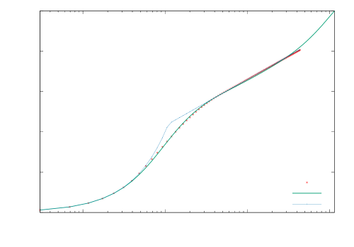
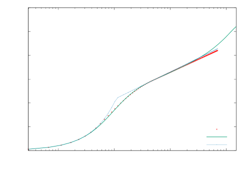
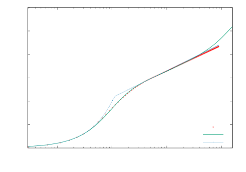
The profiles of the new model are compared to the classical wall laws: $\bm{\widetilde{u}}=z\widetilde{U}_{\tau}^{2}/\nu$ in the viscous sublayer, and $\bm{\widetilde{u}}=u_{\tau}\left(\frac{1}{\kappa}\ln(z\frac{\widetilde{U}_{\tau}}{\nu})+B\right)$ above the viscous sublayer, where the constants $\kappa$ and $B$ are optimally set from the data. These results are shown in figures 2–4 for $Re_{\tau}=1306$, $1437$, $1709$, and $1989$ respectively.

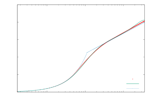
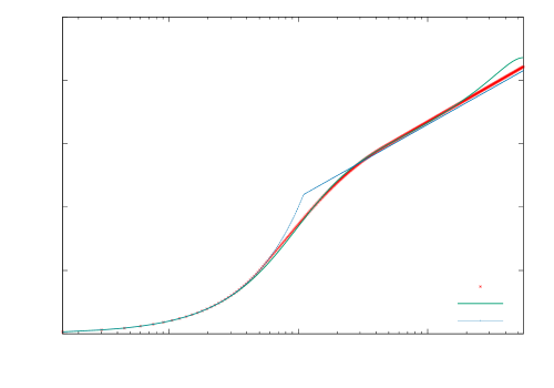
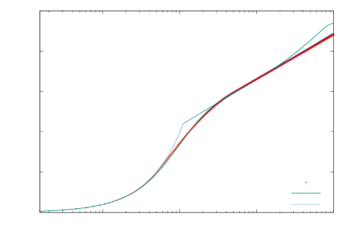
In the viscous sublayer, there is no difference between the classical models and the new one (16). Both of them perfectly superimpose with the reference data. In that region, the variance tensor along the wall-normal direction, $a_{zz}$, is zero.

In the buffer region, where $a_{zz}(z)$ is linear, there is no theoretically well grounded model available for the velocity profile. In this transition area both the classical linear profile or the logarithmic profile deviate significantly from the reference profiles. At the opposite, the new model fits well the data t all the Reynolds number investigated. The LU model, unlike adhoc formulation (Spalding, 1961), enables us to devise a physically coherent model, in which a modified advection ensuing from the unresolved velocity inhomogeneity plays a fondamental role.

In the logarithmic region, both the classical log-law model and the LU model perform similarly and provide very good results for $Re_{\tau}=1306$ and $1437$. For higher Reynolds number ($Re_{\tau}=1709$, and $1989$) they both still match very the data; however the LU log profile approaches even better the data. The good performance of the LU mean velocity profile support the validity of the wall-normal variance tensor profile in the turbulent layer (e.g. linear and square-root profiles of $a_{zz}(z)$ in the buffer zone and in logarithmic layer respectively) as the velocity profile highly depends on $\partial_{z}a_{zz}\partial_{z}\bm{\widetilde{u}}(z_{l})$ (13a).

III.2 Pipe Flow

Let us now examine the results obtained for the pipe flows data. The optimal parameters are shown in table 2. We observe that the value of the viscous layer thickness ($z_{0}^{+}$) decreases with the increase of the friction Reynolds number, while the limit of the buffer zone ($z_{L}^{+}$) grows; the constant $\widetilde{\kappa}$ remains almost constant except for the first simulation associated to the lowest friction Reynolds number.

The mean velocity profiles are plotted in figures 6,6, 8, and 8. As previously, the modified LU model is shown in red, and is compared to the DNS data and the classical logarithmic and viscous velocity profiles. Let us note that compared to turbulent boundary layer flows, pipe flows exhibits a much shorter layer with a logarithmic profile. In the same way as in the turbulent boundary layer case, we clearly see that the model proposed is almost perfectly in agreement with the data up to the end of the logarithmic layer. This model is again particularly relevant for the buffer zone, where no physical model has been yet derived in the literature from a classical eddy-viscosity concept.

Table 2: Parameters value of the mean velocity profile for pipe flows

$Re_{\tau}$	$z_{0}^{+}$	$z_{L}^{+}$	$\widetilde{\kappa}$
180	5.61	43.75	0.150
360	5.27	43.85	0.158
550	5.11	46.31	0.158
1000	5.05	49.00	0.158

Figure 5: Velocity profiles for the pipe flow at $Re_{\tau}=180$. The green curve is the DNS reference velocity profile; the blue dot lines show the classical laws (linear then logarithmic) and the red dots corresponds to the profile of the model under location uncertainty.

Figure 6: Velocity profiles for the pipe flow at $Re_{\tau}=360$. The green curves is the DNS reference velocity profile; the blue dot lines show the classical laws (linear then logarithmic) and the red dots corresponds to the profile of the model under location uncertainty.

Figure 7: Velocity profiles for the pipe flow at $Re_{\tau}=550$. The green curve is the DNS reference velocity profile; the blue dot lines show the classical laws (linear then logarithmic) and the red dots corresponds to the profile of the model under location uncertainty.

Figure 8: Velocity profiles for the pipe flow at $Re_{\tau}=1000$. The green curve is the DNS reference velocity profile; the blue dot lines show the classical laws (linear then logarithmic) and the red dots corresponds to the profile of the model under location uncertainty.

III.3 Channel flow

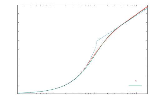
The last example concerns the channel flow at $Re_{\tau}=5200$ of Lee and Moser (2015). For this flow the parameters estimated from the data are gathered in table 3.

Table 3: Parameters value of the mean velocity profile for a channel flow

$Re_{\tau}$	$z_{0}^{+}$	$z_{L}^{+}$	$\widetilde{\kappa}$
5200	5.0	45.0	0.16

As it can be observed they are sensibly the same with a shorter buffer region than in the previous examples.

Figure 9: Mean velocity profiles for the channels flow at $Re_{\tau}\approx 5200$ Lee and Moser (2015). The green curve is the DNS reference velocity profile; the blue dot lines show the classical laws (linear then logarithmic) and the red dots corresponds to the profile of the model under location uncertainty.

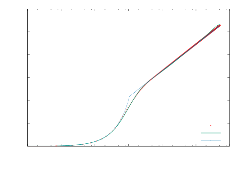
The plot of the mean velocity profiles is shown figure 9. As previously, the LU model explains very well the data. In the buffer zone the LU model almost perfectly match the data. In the the logarithmic region the LU logarithmic law and the classical one perform identically.

IV Conclusion

The modeling under location uncertainty provides a novel expression of the wall-law velocity profiles. For three different wall-bounded flow configurations, going from moderate to high Reynolds numbers, it is shown that the LU model allows us to devise a physical model for the mean velocity profile that matches very well the data in the whole turbulent boundary layer while remaining continuous and differentiable. The derivation unveils in particular the role played by the advection correction due to turbulence inhomogeneity in the transitional zone between the viscous and the logarithmic sublayers. This model is very promising as it provides – as far as we know – for the first time a physically relevant model for the buffer region. The LU derivation relies on a random modeling of the fluctuation velocity fields and exhibits a tensor playing the role of a matrix valued eddy-viscosity term generalizing de facto the Boussinesq assumption and the Prandlt mixing length. This tensor corresponds to the fluctuation variance times a decorrelation time; its wall-normal component is null in the viscous zone, linear in the buffer zone and scales as $\sqrt{z^{+}}$ in the logarithmic layer. The inhomogeneity of this tensor enforces a modified advection term which can be interpreted as the statistical influence of the fluctuation inhomogeneity on the large-scale advection component. This modification has a major contribution in the transitional buffer zone. The new velocity profile associated to the LU model relies principally on a new parameter related to the slope of the variance tensor wall-normal component in the buffer zone.

This new model opens very exciting perspectives for the set up of models “à la” Monin-Obukhov for fluid flows with thermal stratification as well as the establishment of more accurate wall functions for Large Eddy Simulation. It can also be promising for industrial problems involving pipe flows.

References

- Prandtl (1925) L. Prandtl, “Bericht über untersuchungen zur ausgebildeten turbulenz,” Z. Angew. Math. Mech. 5, 136–139 (1925)
- von Karman (1930) T. von Karman, “Meckanishe ähnlichkeit und turbulenz,” Gött. Nachr. , 58–76 (1930)
- Jiménez and Moser (2007) Javier Jiménez and Robert D Moser, “What are we learning from simulating wall turbulence?” Phil. Trans. R. Soc. A 365, 715–732 (2007)
- Marusic et al. (2010) I. Marusic, B. McKeon, P. Monkevitz, H. Nagib A. Smits, and K. Sreenivasan, “Wall-bounded turbulent flows: recent advances and key issues,” Phys. Fluids 22 (2010)
- Klewicki (2010) J. C. Klewicki, “Reynolds number dependence, scaling, and dynamics of turbulent boundary layers,” Trans. ASME J. Fluids Eng. 132, 1–48 (2010)
- Marusic et al. (2013) I. Marusic, J. Monty, M. Hultmark, and A. Smits, “On the logarithmic region in wall turbulence,” J. Fluid Mech. 716, 1–11 (2013)
- Reeks (1983) M. Reeks, “The transport of discrete particles in inhomogeneous turbulence,” J. Aerosol Sci. 14, 729–739 (1983)
- Andrews and McIntyre (1978) D. Andrews and M. McIntyre, “Nonlinear waves on a lagrangian-mean flow,” J. Fluid. Mech. 89, 609–646 (1978)
- Mémin (2014) E. Mémin, “Fluid flow dynamics under location uncertainty,” Geophys. & Astro. Fluid Dyn. 108, 119–146 (2014)
- Chandramouli et al. (2018) P. Chandramouli, D. Heitz, S. Laizet, and E. Mémin, “Coarse large-eddy simulations in a transitional wake flow with flow models under location uncertainty,” Comp. & Fluids 168, 170–189 (2018)
- Kadri Harouna and Mémin (2017) S. Kadri Harouna and E. Mémin, “Stochastic representation of the Reynolds transport theorem: revisiting large-scale modeling,” Computers & Fluids 156, 456–469 (2017)
- Resseguier et al. (2017a) V. Resseguier, E. Mémin, D. Heitz, and B. Chapron, “Stochastic modelling and diffusion modes for proper orthogonal decomposition models and small-scale flow analysis,” J. Fluid Mech. 828, 29 (2017a)
- Resseguier et al. (2017b) V. Resseguier, E. Mémin, and B. Chapron, “Geophysical flows under location uncertainty, Part I Random transport and general models,” Geophys. & Astro. Fluid Dyn. 111, 149–176 (2017b)
- Resseguier et al. (2017c) V. Resseguier, E. Mémin, and B. Chapron, “Geophysical flows under location uncertainty, Part II Quasi-geostrophy and efficient ensemble spreading,” Geophysical and Astrophysical Fluid Dynamics 111, 177–208 (2017c)
- Resseguier et al. (2017d) V. Resseguier, E. Mémin, and B. Chapron, “Geophysical flows under location uncertainty, Part III SQG and frontal dynamics under strong turbulence conditions,” Geophysical and Astrophysical Fluid Dynamics 111, 209–227 (2017d)
- Holm (2015) D.D. Holm, “Variational principles for stochastic fluid dynamics,” Proc. R. Soc. A 471 (2015)
- Crisan et al. (2017) D. Crisan, F. Flandoli, and D. Holm, “Solution properties of a 3d stochastic euler fluid equation,” arXiv:1704.06989 [math-ph] (2017)
- Cotter et al. (2017) C.J. Cotter, G.A. Gottwald, and D.D Holm, “Stochastic partial differential equations as a diffusive limit of deterministic Lagrangian multi-time dynamics,” Proc. R. Soc. A 473: 20170388 (2017)
- Jimenez (2018) J. Jimenez, “Coherent structures in wall-bounded turbulence,” J. Fluid. Mech. 842, 1–100 (2018)
- Sillero et al. (2013) J.A. Sillero, J. Jiménez, and R.D. Moser, “One-point statistics for turbulent wall-bounded flows at reynolds numbers up to ,” Physics of Fluids 25, 105102 (2013)
- M. P. Simens J. Jimenez (2009) Y. Mizuno M. P. Simens J. Jimenez, S. Hoyas, “A high-resolution code for turbulent boundary layers,” Journal of Computational Physics 228, 4218–4231 (2009)
- G. Borrell (2013) J. Jimenez G. Borrell, J.A. Sillero, “A code for direct numerical simulation of turbulent boundary layers supercomputers,” Computers & Fluids 80, 37–43 (2013)
- El Khoury et al. (2013) G.K. El Khoury, P. Schlatter, A. Noorani, P.F. Fischer, and A. V Brethouwer, G.and Johansson, “Direct numerical simulation of turbulent pipe flow at moderately high reynolds numbers,” Flow, turbulence and combustion 91, 475–495 (2013)
- Lee and Moser (2015) M. Lee and R.-D. Moser, “Direct numerical simulation of turbulent channel flow up to ,” J. Fluid Mech. 774, 395–415 (2015)
- Spalding (1961) D. B. Spalding, “A single formula for the “law of the wall”,” J. of Applied Mech. 28, 455–458 (1961)