PARIS: Predicting Application Resilience Using Machine Learning

Abstract.

Extreme-scale scientific applications can be more vulnerable to soft errors (transient faults) as high-performance computing systems increase in scale. The common practice to evaluate the resilience to faults of an application is random fault injection, a method that can be highly time consuming. While resilience prediction modeling has been recently proposed to predict application resilience in a faster way than fault injection, it can only predict a single class of fault manifestation (SDC) and there is no evidence demonstrating that it can work on previously unseen programs, which greatly limits its re-usability.

We present PARIS, a resilience prediction method that addresses the problems of existing prediction methods using machine learning. Using carefully-selected features and a machine learning model, our method is able to make resilience predictions of three classes of fault manifestations (success, SDC, and interruption) as opposed to one class like in current resilience prediction modeling. The generality of our approach allows us to make prediction on new applications, i.e., previously unseen applications, providing large applicability to our model. Our evaluation on 125 programs shows that PARIS provides high prediction accuracy, 82% and 77% on average for predicting the rate of success and interruption, respectively, while the state-of-the-art resilience prediction model cannot predict them. When predicting the rate of SDC, PARIS provides much better accuracy than the state-of-the-art (38% vs. -273%). PARIS is much faster (up to 450x speedup) than the traditional method (random fault injection).

1. Introduction

High-performance computing (HPC) systems are increasingly used to run large scientific applications that simulate real-world phenomena. These applications are expected to compute precise and correct numerical answers for a large set of science and engineering problems. As HPC systems increase in scale, they become more susceptible to soft errors (Baumann, 2005) (also known as transient faults) due to feature size shrinking, lower voltages, and increasing densities in hardware infrastructures (Sridharan et al., 2015). As a result, scientific applications running at extreme scale must apply different resilience methods to tolerate frequent soft errors. Applying these methods to a given application often requires a deep understanding of the degree of resilience of the application.

The common practice to study application resilience to errors in HPC system is Fault Injection (FI) (Xu and Li, 2012; Wei et al., 2014; Cher et al., 2014; Calhoun et al., 2014; Venkatagiri et al., 2016; Georgakoudis et al., 2017; Kumar Sastry Hari et al., 2017; Kaliorakis et al., 2017; Li et al., 2012). This approach uses a large amount of random FIs, each of which randomly selects an instruction, and then triggers bit flips at the instruction input or output operands during application execution. Statistical results are then used to quantify application resilience. A typical analysis is, for example, to measure the percentage of times a fault yields silent data corruption (SDC) in the output of the program.

While FI works in practice and is widely used in resilience studies, a key problem of this approach is that it is highly time consuming, and as a result it is usually applied to limited scenarios, for example, on applications that run for a short period of time and/or single-threaded codes. To illustrate the problem, consider an application that runs for 6 hours—a typical execution time for a large-scale scientific simulation. Using statistical analysis (e.g., using (Leveugle et al., 2009)), the number of random FIs to obtain a low margin of error (e.g., 1%-3%) is in the order of thousands of injections. Thus, the total FI campaign could last several days. For multi-threaded or multi-process applications, this time is much higher since random faults must be injected in different threads or processes.

Since FI is too time consuming to measure application resilience, recent work proposed the idea of predicting application resilience using an error-propagation model, as opposed to measuring application resilience via FI. The idea is to build a model that explains how errors in instructions propagate to the program output and then use the model to estimate the percentage of times SDC occurs. Here, resilience prediction avoids running the code multiple times (as in traditional FI) at the price of being sometimes less accurate than FI. The most recent work on this domain is Trident (Li et al., 2018), which uses an analytical model to predict the rate of SDC for a given application and input.

While the Trident approach is a useful first step in the direction of application resilience prediction, it has some limitations. First, the approach predicts only a specific class of fault manifestation, SDC. Usually when analyzing the resilience of an application, scientists are interested in understanding at least three classes of fault manifestations: (1) SDC, (2) interruptions (i.e., crashes or hangs), and (3) success (i.e., the fault was benign and did not affect the program output). Because of the low-level analytical modeling approach of Trident, it cannot predict all of these three cases. Second, resilience predictions are made on the program that was used to build the model and there is no evidence demonstrating that it can work on previously unseen programs, which greatly limits the re-usability of the model.

Paper Contributions. We present PARIS, an approach for fast and accurate prediction of application resilience. PARIS avoids the time-consuming process of randomly selecting and executing many injections that FI incurs. Using machine learning and a large set of representative programs and kernels as the input, we build a generic model that explains how error masking and error propagation occur within code regions. Once the model is trained, it can be used to predict three classes of fault manifestations—SDC, interruptions and success—for a new, previously unseen application, addressing the major limitations of Trident.

Our machine learning modeling is unique and is based on several key principles. First, we aim at building a model that captures the implicit relationship between application characteristics and application resilience, which is difficult to capture for analytical models, such as (Li et al., 2018). Second, we carefully choose application characteristics as features for the model; we select features that are directly related to application resilience and that capture the order of execution of instructions as we found that the latter is critical in accurately modeling error propagation. Third, we perform sophisticated feature reduction to enable efficient model training. Fourth, we perform a large model-selection search among 18 different widely-used models—while regression is the most natural choice of modeling for our problem, there are a number of regression models, thus we must answer which model can provide the best accuracy.

In summary, our contributions are as follows.

• We present PARIS, the first machine learning-based approach to predict application resilience; we find that our approach is up to 450x faster than the traditional FI approach.

• We describe a framework to build machine leaning models that can predict more classes of fault manifestations than the state-of-the-art resilience prediction method, Trident
   (Li et al., 2018): three in our case (SDC, interruptions, and success) versus one (SDC) on Trident. Our prediction accuracy for SDC is better than Trident (38% vs. -273% on average). Our prediction accuracy for success and interruptions prediction is 82% and 77%, with a variation of 0.02 and 0.05, respectively, while Trident cannot predict those cases.

• We design and demonstrate that our modeling method can predict application resilience on previously unseen applications, i.e., applications that were not used on the modeling phase, which current methods cannot do.

Our evaluation methodology is solid and comprehensive. We use in total of 125 programs, 18 machine learning models and perform 375,000 FIs to compare our results to those of traditional random FI, using a confidence interval of 99% and a margin error of 1%. To the best of our knowledge, we are the first on providing such a compressive evaluation for a resilience prediction method.

2. Background

We present useful background information and definitions before presenting our approach.

2.1. Fault Model

We consider soft errors (Baumann, 2005), i.e., transient faults that escape from hardware protection and propagate to the application level. These errors manifest as bit flips in registers and memory locations. Corrupted registers and memory cells are consumed by the application. We refer to any of these registers and memory locations as a location in the paper.

We focus on single-bit errors, not multi-bit errors. The reason behind this is that (1) single-bit errors are the most common soft errors—multi-bit errors rarely happen in large-scale systems (Bautista-Gomez et al., 2016); (2) in many cases, multi-bit errors have the similar impact on the application as single-bit errors (Sangchoolie et al., 2017).

Fault injection. We use PINFI (Wei et al., 2014) to perform fault injections into programs. Comparing with LLFI (Thomas and Pattabiraman, 2013) and REFINE (Georgakoudis et al., 2017) (two common FI tools), PINFI (Wei et al., 2014) is more accurate than LLFI and comparable to REFINE for FI.

Figure 1. Overview of PARIS and the workflow of the training process in our machine learning model.

2.2. Application Resilience

We run FI campaigns to measure the application resilience. A FI campaign contains many FIs. In each FI, a single-bit error is injected into an input/output operand of an instruction. A location can be an operand of any instruction.

We classify the outcome, or manifestation, of programs corrupted by bit flips into three classes: success, SDC, and interruption:

• Success: the execution outcome is exactly the same as the outcome of the fault-free run. The execution outcome can also be different from the outcome of the fault-free run, but the execution successfully passes the result verification phase of the application.

• SDC: the program outcome is different from the outcome of the fault-free execution, and the execution does not pass the result verification phase of the application.

• Interruption: the execution does not reach the end of execution, i.e., it is interrupted in the middle of the execution, because of an exception, crash, or hang.

Rates. To quantify the application resilience in a given FI campaign, we measure the rate of each of the three classes of manifestations described above. In particular, we use the formula:

(1) $$\text{\#Manifestations}/N,$$

where #Manifestations is the number of times a given class of manifestation (success, SDC or interruption) occurs, and $N$ is the number of FIs performed in a FI campaign. In this paper, we consider the rates of success, SDC and interruption as metrics to quantify application resilience.

2.3. Features and Machine Learning Models

Features. A feature is an application characteristic. Multiple features construct a feature vector, $v$, which is used as the input for our machine learning models. Choosing discriminative features is an essential task for building an effective machine learning model. However, irrelevant and redundant features can affect the modeling accuracy, thus we must perform feature selection on the modeling process.

Models. There are two classes of machine learning models: classification and regression. Our problem is naturally a regression problem since the manifestation rates are real numbers. More formally, our problem is to find a model $f()$, for which given an feature vector $v$ corresponding to an application $A$, $f(v)$ gives us the rates of SDC, interruption, and success for $A$. Note that the SDC, interruption, and success rates are real numbers between 0.0 and 1.0. Since they are mutually exclusive events, the addition of them for a given application is 1.0.

Prediction Accuracy. After our model is trained, it is used to predict application resilience. To estimate the prediction accuracy of the model, we compute the relative error between the predicted application resilience and the application resilience that we observe by performing FI. The prediction accuracy $P_{\textit{accuracy}}$ is defined as follows:

(2) $$P_{\textit{accuracy}}=1-\frac{|P_{\textit{rate}}-O_{\textit{rate}}|}{O_{\textit{rate}}},$$

where $P_{\textit{rate}}$ is the predicted rate (of either the success, SDC or interruption), and $O_{\textit{rate}}$ is the observed rate by performing FI. A perfect model has a $P_{\textit{accuracy}}$ of 1.0.

Training and Testing Phases. The modeling process of machine learning includes training and testing. We use a set of representative applications to train the model—once it is trained, the model is used to predict, or test, the manifestation rates on new applications. We call the applications used for training and testing the training dataset and the testing dataset, respectively.

3. Overview

We give a high-level overview of PARIS. Figure 1 depicts the workflow of the training process in PARIS. The most challenging part of the training process is to construct features relevant to application resilience and producing high modeling accuracy.

Features Construction. We use instruction type and number of instruction instances for each type as features. A static instruction in a program has an instruction type (opcode), and can be executed many times, each of which is an instruction instance. Using the number of instruction instances for each instruction type as a feature will result in too many features, which demands a large training dataset. To reduce the number of features, we group all instruction types (65 in total) into four groups: control flow instructions, floating point instructions, integer instructions, and memory-related instructions. For each instruction group, we count the number of instruction instances as a feature.

Furthermore, we use six resilience computation patterns proposed in (Guo et al., 2018) as features. Among the six patterns, four of them (conditional statement, shifting, data truncation, and data overwriting) are individual instructions that cannot be grouped into the four instruction groups. Two of them (dead locations and repeated addition) include multiple instructions and those instructions together (not individual instructions) contribute to application resilience.

Counting dead locations and repeated addition from the dynamic instruction trace is challenging because we must repeatedly search within the trace to find correlation between instructions. To detect dead locations, we use a technique that caches intermediate results of trace analysis to avoid repeated trace scanning. To detect repeated addition, we build a data dependency graph for addition instructions. Such graph enables easy detection of repeated addition.

Because different instruction instances can have different capabilities to tolerate errors, even though they have the same instruction type (or the same resilience computation pattern), we introduce resilience weight when counting instruction instances. The resilience weight gives each instruction instance a weight quantifying the possible number of single-bit errors that can be tolerated by the instance.

Furthermore, we introduce execution order information as a feature. We notice that instruction order can affect the application resilience. However, representing the order information of all instruction instances as a feature is a challenge. We use N-gram (Brown et al., 1992; Cavnar et al., 1994), a technique commonly used for processing speech data, to capture the order information.

Machine Learning Techniques. There are many machine learning models we can use for PARIS. We use a model selection method (Kohavi, 1995) to find the machine learning model with the highest prediction accuracy. We also use the filtering-based feature selection (Das, 2001) to filter out irrelevant and redundant features. As used in the existing machine learning work, we use model tuning techniques including whitening, bagging, and hyperparameter tuning to improve the prediction accuracy of our model.

Use of PARIS. To use PARIS, users do not need doing FI. Instead, users generate a dynamic instruction trace and feeds it to PARIS. PARIS will output a numerical value, which is the predicted success, SDC, or interruption rate.

4. Design

We describe the design details in this section.

4.1. Feature Construction

To construct features for the regression models, we have the following requirements: (1) The features should be relevant to application resilience. (2) The number of features should be small enough. Ideally, the number should be much smaller than the number of applications for training to avoid under-determination of the model. (3) We should avoid redundant and irrelevant features. Those features can lower prediction accuracy. We describe our feature construction following the above requirements in this section.

4.1.1. Instruction Groups

The first features we introduce into the models are the instruction type and number of instruction instances in each type. These features are highly relevant to application resilience. For example, recent studies (Elliott et al., 2013; Menon and Mohror, 2018; Li et al., 2018) reveal that floating point instructions make application resilient to faults, because the faults in mantissa bits of floating point numbers are often ignorable by the application (especially HPC applications). Load/store instructions also has significant impact on application resilience, because the computation following load/store instructions may need those loaded/stored values.

We use the LLVM compiler (Lattner and Adve, 2004) to build applications, which is architecture independent, allowing us to build a more general and reusable model for resilience prediction. We enumerate all LLVM IR instructions and get 65 instruction types. However, building a feature vector with 65 instruction types will lead to at least 65 unknown variables in the solution space. To fill up the solution space, it could easily require thousands of applications (Chen et al., 2017; Domingos and Hulten, 2000) to train the models. This violates the requirement (2) and can be time-consuming to find the optimal solution.

To address this problem, we group 65 instruction types into four groups based on the functionality of instructions to reduce the number of features. Instruction functionality relies on instruction types; different instruction types have different impacts on application resilience. For example, we group control flow related instructions (e.g., Br and Select) into a group, and group floating point instructions (e.g., Fadd and Sine) into a group. Table 1 lists the four groups, including control flow instructions, floating point instructions, integer instructions, and memory-related instructions.

For each instruction group, we count the number of instruction instances from the dynamic instruction trace, and then normalize the number based on the total number of instruction instances. We normalize the number as a feature to make the feature value independent of the size of the dynamic instruction trace.

Table 1. Four groups of instruction types and three resilience patterns as features to build the machine learning models.

Group Name	Instruction types
Control Flow Instructions (CFI)	Br, Indirectbr, Select, PHI, Fence, DMAFence, Call
Floating Point Instructions (FPI)	Fadd, Fsub, Fmul, Fdiv, Frem, Cosine, Sine
Integer Instructions (II)	add, sub, mul, Udiv, Sdiv, Urem, Srem
Memory-related Instructions (MI)	Load, Store, DMAStore, DMALoad, Getelementptr, ExtractElement, InsertElement, ExtractValue, InsertValue, FPToUI, FPToSI, UIToFP, SIToFP, PtrToInt, IntToPtr, AddrSpaceCast
Pattern name	Instruction types
Condition	ICmp, FCmp, Switch, And, Or, Xor
Shift	Shl, LShl, AShl
Truncation	Trunc, ZExt, Sext, FPTrunc, BitCast, FPExt

4.1.2. Using Resilience Computation Patterns as Features

The recent work (Guo et al., 2018) finds six resilience computation patterns strongly related to application resilience. The resilience computation pattern is defined as combinations or sequences of computations that make an application naturally resilient. These six patterns are dead locations, repeated addition, conditional statements, shifting, data truncation, and data overwriting. We introduce the patterns of dead locations and repeated addition as features, because the two patterns include multiple instructions and those instructions together (not individual instructions) contribute to application resilience; The other four patterns are individual instructions and could fall into the four instruction groups. However, we use them separately as features, because of their significance to application resilience (Guo et al., 2018).

We describe how to introduce the six patterns as features as follows. A pattern can be repeatedly executed by the application. We name the execution of a specific pattern within the application as the pattern instance. To introduce these six patterns as features, we could simply count the number of the pattern instances for each pattern. However, doing so has a couple of challenges.

First, counting the number of the pattern instances for dead locations and repeated addition can be time-consuming, because we have to find correlations between instructions to determine if the location is dead or if the addition repeatedly happens to the same variable. Doing so requires iteratively scan the dynamic instruction trace. We discuss how to efficiently count the number of the pattern instances for the two patterns in Section 4.1.3 and Section 4.1.4, respectively.

Second, for the patterns of conditional statements, shifting, data truncation and data overwriting that are represented as individual instructions (see the last three rows in Table 1 for these instructions), simply counting the number of pattern instances cannot discriminate the fault tolerance capabilities of different pattern instances. For example, the fault tolerance capability of the “shifting” pattern (a pattern involving a shift instruction) depends on how many bits are shifted. A shift instruction instance shifting three bits can tolerate three single-bit errors, while a shift instruction instance shifting one bit can tolerate one single-bit error. To distinguish the fault tolerance capabilities of different instruction instances, we introduce weights (named resilience weight) for counting instances of the patterns. Besides introducing weights for the patterns of conditional statements, shifting, data truncation and data overwriting, we also introduce weights to instructions whose instances can also have different fault tolerance capabilities. We describe how we determine weights for instruction instances in Section 4.1.5.

4.1.3. Extracting the Feature of Dead Location

Dead locations refer to those locations that have short live time. While the errors in those locations can propagate to one (or a few) other locations, many of the dead locations are not used anymore. As a result, the total number of corrupted locations in the program can decrease, because of those short live locations. A code region with a higher percentage of dead locations (i.e., the number of dead locations over the number of total locations) has higher resilience.

To efficiently detect dead locations and calculate the percentage of dead locations, we split the dynamic instruction trace into chunks and pre-process the chunks before detecting dead locations. During the trace pre-processing, we analyze instructions in each chunk and record names of locations within the chunk. This location record is saved in an array for each chunk. To determine if a location in a chunk is a dead location, we only need to check whether the same location is used in any following chunks by examining the arrays. If the location is not used, then the location is a dead location. In essence, the arrays for chunks save instruction analysis results to avoid repeatedly scanning the trace and analyzing instructions. For each chunk, we normalize the number of dead locations by the total number of locations within the chunk and compute the percentage of dead locations for the chunk. We use the average dead location rate of all chunks as a feature.

4.1.4. Extracting the Feature of Repeated Addition

Repeated addition refers to the addition repeatedly happening to a variable, such that the error in the variable can be amortized. To decide if an addition instruction is a part of repeated addition, we must first decide if the addition instruction is involved in a self addition. The self addition is that a location adds other location(s) to itself. The pseudo code in Figure 2 gives an example of self addition.

To detect a self addition, we first construct a data dependency graph for addition operations. A node in the graph is a location; edges between graph nodes represent data dependency. Then, given an addition instruction, we examine the output operand of the addition instruction, and decide if the location (the output operand) is a source operand of a previous addition operation by backward traversing the graph.

Figure 2 illustrates how a data dependency graph looks like and how a self addition is found. In the example, we have four addition statements (operations) in a for loop. The location $a$ appears as the output of the last addition statement ($a=b+c$ in Line 9). To determine if the addition statement is involved in a self addition, we find the node 0 corresponding to $a$ in the data dependency graph. We traverse the graph backward, and find $a$ appears in a previous node, the node 7. The node 7 corresponds to a source operand of a previous addition statement ($e=a+4$). Hence, a self addition is detected. A repeated addition is composed by a number of self additions.

To use repeated addition as a feature, we normalize the number of repeated addition instances by total number of instruction instances. This makes the feature value independent of the size of the dynamic instruction trace.

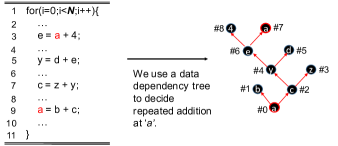
Figure 2. An example to detect repeated additions.

4.1.5. Resilience Weight

Given an instruction, all bit locations of its input and output operands are subject to error corruption. The resilience weight ($\mathcal{R}{es}$) of an instruction is defined as follows.

(3) $$\mathcal{R}{es}=\frac{\#bit\ locations\ that\ tolerate\ errors}{\#ofall\ bit\ locations}$$

Using the right-shift instruction as an example. The instruction has three 8-bit operands and in total 24 locations. Assume that an instance of the instruction shifts four least significant bits of an operand. The shifted four bits can tolerate four single-bit errors. Also, the eight bits in the output operand of the instruction can tolerate errors because of the result overwriting in the output operand. Hence, in this example, the resilience weight for this instruction instance is (4+8)/24 = 0.5.

For any floating point and integer instruction, the bit locations that can tolerate errors are the bit locations of the output operands, because we expect errors in the output operands can be overwritten by the instructions.

When counting the number of instruction instances or the number of pattern instances, we use the weights to account the numbers.

Putting All Together. As a result of the above feature construction, we construct a feature vector of ten features, formulated in Equation 4. The notation of the equation can be found in Table 1.

(4) $$\mathcal{F}^{ave}_{10}=[CFI,FPI,II,MI,\\ Condition,Shift,Truncation,DO,DLR,RA]$$

We call $\mathcal{F}^{ave}_{10}$ the foundation feature vector and call the ten features foundation features in the rest of the paper.

4.2. Including Instruction Order

The foundation features are not good enough to achieve high prediction accuracy. In particular, the foundation features lack instruction order (i.e., the execution order) information. Capturing the instruction order is important, because it matters to error propagation.

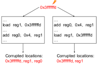
Figure 3. An example to show that the execution order of instructions matters to error propagation.

To give an intuition of why the execution order matters, we use a simple example shown in Figure 3. In this example, we have a $load$ instruction and an $addition$ instruction. Assume that an error happens on a memory address 0x3ffffffd. If the $load$ instruction happens first, then the erroneous value in the memory address can propagate to the locations $reg1$ and $reg0$. but if the $addition$ instruction happens first, then the erroneous value in the memory address can only propagate to the location $reg1$. This example is a demonstration of how the execution order matters to error propagation.

To introduce execution order information into the feature vector, we use the “N-gram” technique. The N-gram is a technique used in computational linguistics. It can work on a sequence of streaming words, and predict next word using sequences of previous words. N-gram can capture the word order information. In particular, every $n$ continuous words composes a $n-$gram ($n=1,2,3,...$). We can introduce the order information into features by using the N-gram.

In particular, we partition the dynamic instruction trace into chunks (each chunk is a gram). Each chunk is treated as a “word”, and the sequence of chunks is processed as the sequence of words. For each chunk, we collect ten foundation features, and build a foundation feature vector of size ten for each chunk. Then, we build an average foundation feature vector (denoted as $\mathcal{F}^{ave}_{10}$) whose feature values are the average values of foundation feature vectors of all chunks.

Furthermore, we combine every two chunks to build a 2-gram (or bigram in the language of N-gram). For each bigram, we combine two foundation feature vectors to build a 2-gram feature vector of size 20. After that, we build an average 2-gram feature vector (denoted as $\mathcal{F}^{ave}_{20}$) for all bigrams. $\mathcal{F}^{ave}_{20}$ is the average value of all 2-grams feature vectors; $\mathcal{F}^{ave}_{20}$ has a size of 20.

After that, we have $\mathcal{F}^{ave}_{10}$ of size 10 and $\mathcal{F}^{ave}_{20}$ of size 20. The new feature vector with the execution order information is a combination of $\mathcal{F}^{ave}_{10}$ and $\mathcal{F}^{ave}_{20}$. The new feature vector has a size of 30. We denote the new feature vector $\mathcal{F}^{ave}_{30}$ Figure 4 depicts how we build the feature vector with the execution order information included.

We do not consider trigram (i.e., 3-gram) or higher gram, because common practices (Pei et al., 2014; Chen et al., 2015) demonstrate that there is no need to use higher grams than bigram. In (Chen et al., 2015), bigram achieves better accuracy than trigram. Using trigram or higher grams does not provide much improvement in prediction accuracy, but dramatically increases the feature vector size and increases the complexity of model training.

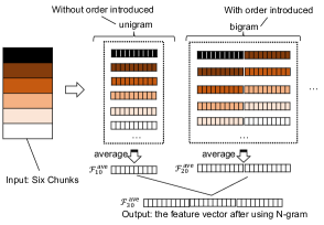
Figure 4. Applying the N-gram technique to introduce the execution order information.

4.3. Models Selection

There are tens of regression models. Each of them has pros and cons, and can be fit to different scenarios. We explore 18 most common regression models.

We use cross-validation to evaluate 18 regression models on the training dataset to select the best models. CV partitions the dataset into $p$ folds. $q$ of $p$ folds are used for training, while the remaining $p-q$ folds are used for testing. There are $p/(p-q)$ rounds of training/testing. In each round, different $p-q$ folds are used for testing. We choose the regression models that have the highest prediction accuracy (on average) among all testing dataset.

In our study, we choose top five regression models based on CV. The five models are shown in Table 2. Among the remaining 13 models, 12 of them have very poor prediction accuracy (the prediction accuracy is even negative, based on the calculation of Equation 2); one of them (i.e., the decision tree) is just a special case of one of the top five (the random forest) in nature. For the five selected models, we improve their model accuracy as follows.

4.4. Feature Selection

After the five models are selected, we explore the possibility to reduce the feature vector size for each of those models. Reducing the feature vector size is useful to eliminate those irrelevant and redundant features to improve modeling accuracy.

We use three common techniques to select features: variance, p-value, and mutual information. Simply speaking, the variance of a feature measures the variance of feature values across different input code; The p-value is metric that that measures the significance level between a feature and the modeling result (i.e., the success, SDC, or interruption rate); The mutual information measures the mutual dependency between a feature and the modeling result.

Using the above method, we sort features into a list. In total, we have three lists, each of which corresponds to one of the three techniques. We design a voting strategy based on the combination of the three lists. In particular, each feature in a list has an index. For each feature, we add its three indexes to get a global index. We sort the features again based on the global index. We choose the best $k$ (where $k=2,3,...,30$) features according to their prediction accuracy. Such voting strategy and feature selection algorithm (Liu et al., 2016; Zhang et al., 2006; Tsymbal et al., 2005) are common in machine learning.

4.5. Model Tuning

After the feature selection process, we further tune the five models. We choose the one with the highest prediction accuracy as the final model. We use the following tuning techniques for model tuning.

Whitening: Whitening (Coates et al., 2011) is commonly used for avoiding domination effects of any features for better generalization to improve the modeling accuracy.

Bagging (Model Averaging): Bagging (Domingos, 2000) is often used for reducing the variance in the training data, so that we can eliminate the effect of bad outliers.

5. Implementation

Dataset Construction. We have multiple requirements on creating training and testing dataset. (1) The training dataset must be large to avoid model underdetermination (i.e., the evidence available is insufficient to identify which belief one should hold about that evidence.); (2) applications used to generate training and testing dataset must have diverse computation and have diverse resilience characteristics. (3) Applications used to generate training dataset must have explicit result verification phases. Having those phases allows us to easily determine the fault manifestation (SDC, interruption, and success).

We use representative benchmark suites and scientific applications to create the testing dataset, including NAS parallel benchmark suite (Bailey et al., 1992), PARSEC benchmark suite (Bienia et al., 2008), CORAL benchmark suite (cor, 2006), Rodinia benchmark suite (Che et al., 2009), SPEC CPU2000 (Henning, 2000), and two scientific applications (Hercules for earthquake simulation (Aktulga et al., 2012) and PuReMD for reactive molecular dynamics simulation (Taborda and Bielak, 2011)). We carefully choose 25 applications from the above benchmark suites and scientific applications for testing. The 25 applications are shown in Table 4. We call the 25 applications big benchmarks in the rest of the paper.

To train PARIS, we use 100 common computation kernels from HackerRank (HackerRank, 2009). These kernels are relatively shorter than the big benchmarks, but these kernels all have explicit verification phases.

Trace Generation. We use LLVM-Tracer (Shao and Brooks, 2013), a tool to generate dynamic LLVM IR traces based on LLVM instrumentation. The trace includes LLVM IR instructions and their operands.

To introduce the execution order information, we define “chunk”; each chunk is the dynamic instruction trace of a loop or code between two neighbor loops. We extend LLVM-tracer to generate a subtrace for each chunk.

Regression Model Selection. We use 10-fold cross validation to evaluate 18 regression models on the training dataset to select the best models. These 18 models are Kneighbors Regression, Gradient Boosting Regression, Random Forest Regression, SV Regression, NuSVR Regression, Decision Tree Regression,SGD Regression, Lasso Regression, Elastic Net Regression, Huber Regression, Bayesian Ridge Regression, Passive-Aggressive Regression, Ridge Regression, KernelRidge Regression, TheilSen Regression, RANSAC Regression, Least Square Linear Regression, and MLP Regression. We use scikit-learn (Pedregosa et al., 2011) to implement the models. Table 2 shows the top five regression models with the highest prediction accuracy. The remaining 13 regression models are not listed because of their low prediction accuracy.

Tuning Hyperparameters. Each regression model has multiple hyperparameters. We leverage “grid-search” (Bergstra and Bengio, 2012) to decide the values of hyperparameters for training.

6. Evaluation

We use the trained regression models to predict the rate of success and interruption. The SDC rate is simply the result of subtracting the rates of success and interruption from one (“1”). We do not use the models to directly predict the SDC rate, because the observed SDC rate ($O_{rate}$ in Equation 2) for some applications can be very small (close to 0), which easily makes $|P_{rate}-O_{rate}|/O_{rate}$ in Equation 2 larger than 1. As a result, $P_{accuracy}$ is negative, which is counter-intuitive (it should be always non-negative).

We evaluate our models and modeling methods from two perspectives: (1) the modeling accuracy; (2) the contributions of various modeling techniques and model optimization techniques to the modeling accuracy.

Table 2. The average prediction accuracy for the three rates (i.e., Success rate=SR, SDC rate=SDCR, and interruption rate=IR). Numbers in the parenthesis are for the variance of the prediction accuracy. Notation: APA=average prediction accuracy, SCK=small computation kernels, HPCB=HPC benchmarks.

Regression models	APA for SR on SCK	APA for SR on HPCB	APA for IR on SCK	APA for IR on HPCB
SV Regression	0.75 (0.15)	0.72 (0.17)	0.71 (0.17)	0.67 (0.24)
Gradient Boosting Regression	0.81 (0.13)	0.82 (0.02)	0.75 (0.15)	0.77 (0.05)
Random Forest Regression	0.77 (0.14)	0.74 (0.02)	0.72 (0.14)	0.71 (0.18)
Kneighbors Regression	0.74 (0.16)	0.7 (0.04)	0.63 (0.21)	0.56 (0.32)
NuSVR Regression	0.75 (0.21)	0.74 (0.08)	0.74 (0.17)	0.66 (0.26)

Table 3. Feature voting scores for each dimension of the feature vector $\mathcal{F}^{ave}_{30}$.

(a) Feature voting scores for predicting the success rate.

Dimension Number	4	24	8	28	17	12	14	22	18	27
Sorted voting score (Smaller is better)	20	22	23	24	25	27	29	29	31	32
Dimension Number	2	3	23	7	20	16	6	21	13	26
Sorted voting score (Smaller is better)	33	39	39	40	43	45	46	48	50	50
Dimension Number	11	1	30	15	5	10	25	29	9	19
Sorted voting score (Smaller is better)	53	54	62	69	70	71	74	74	86	87

(b) Feature voting scores for predicting the interruption rate.

Dimension Number	14	18	4	8	27	24	28	7	30	16
Sorted voting score (Smaller is better)	20	23	24	27	27	32	32	34	37	38
Dimension Number	6	17	10	26	12	13	1	3	11	2
Sorted voting score (Smaller is better)	39	40	42	43	46	46	47	47	52	53
Dimension Number	21	19	20	23	5	15	22	25	9	29
Sorted voting score (Smaller is better)	53	55	55	56	62	63	69	69	77	87

6.1. Prediction Accuracy

We show the prediction accuracy in Table 2 for the top five regression models. We have applied feature selection and model tuning techniques to improve the prediction accuracy of these models. The second and fourth columns of Table 2 show the results from cross-validation. We use the 100 small computation kernels for training. The third and fifth columns of Table 2 show the results from testing. We use the big benchmarks for testing.

Table 4. The detailed prediction results for 25 big benchmarks. Notation: SR=Success Rate; SDCR=SDC Rate; IR=Interruption Rate; Pred.=Prediction; Obs.=Observed; Accy=Accuracy.

Big benchmarks	Suite	Program input	Obs. SR	Pred. SR	Pred. Accy for SR (higher is better)	Obs. SDCR	Pred. SDCR	Pred. Accy for SDCR (higher is better)	Pred. Accy for SDCR by Trident	Obs. IR	Pred. IR	Pred. Accy for IR (higher is better)
IS	NAS	Class S	0.653	0.701	0.926	0.083	0.103	0.020	N/A	0.264	0.195	0.739
LU	NAS	Class S	0.575	0.698	0.787	0.174	0.150	0.863	N/A	0.251	0.152	0.606
Nn	Rodinia	filelist_4 5 30 90	0.513	0.847	0.348	0.173	0.000	0.000	N/A	0.314	0.323	0.973
Myocyte	Rodinia	100 1 0 4	0.741	0.707	0.954	0.022	0.023	0.939	N/A	0.237	0.270	0.862
Backprop	Rodinia	35536	0.670	0.528	0.788	0.016	0.111	-4.946	N/A	0.314	0.361	0.850
CG	NAS	Class S	0.739	0.704	0.953	0.139	0.147	0.941	N/A	0.122	0.149	0.782
MG	NAS	Class S	0.781	0.640	0.820	0.008	0.009	0.835	N/A	0.211	0.351	0.339
BT	NAS	Class S	0.656	0.606	0.924	0.164	0.252	0.465	N/A	0.180	0.142	0.791
SP	NAS	Class S	0.385	0.375	0.974	0.306	0.255	0.832	N/A	0.309	0.371	0.801
DC	NAS	Class S	0.578	0.690	0.806	0.060	0.000	0.000	N/A	0.362	0.396	0.906
Lud	Rodinia	512.dat	0.760	0.669	0.881	0.142	0.135	0.953	N/A	0.098	0.195	0.007
Kmeans	Rodinia	100	0.843	0.712	0.844	0.045	0.093	-0.070	N/A	0.112	0.195	0.256
sAMG	CORAL	aniso	0.467	0.704	0.492	0.370	0.144	0.388	N/A	0.163	0.152	0.933
STREAM	PARSEC	10 20 64 512 512 100 none oput.txt 4	0.723	0.611	0.845	0.066	0.194	-0.938	N/A	0.211	0.195	0.926
Libquantum	SPEC	33 5	0.863	0.922	0.931	0.034	0.000	0.000	0.924	0.103	0.125	0.784
Blackscholes	PARSEC	in_4.txt	0.663	0.571	0.862	0.122	0.203	0.338	0.878	0.215	0.226	0.949
Sad	Parboil	reference.bin frame.bin	0.475	0.498	0.951	0.216	0.314	0.546	0.650	0.309	0.188	0.607
Bfs-parboil	Parboil	graph_input.dat	0.496	0.686	0.617	0.131	0.010	0.079	0.967	0.373	0.304	0.815
Hercules	CMU	scan simple_case.e	0.580	0.610	0.949	0.182	0.172	0.945	-0.282	0.238	0.218	0.917
PuReMD	Purdue Univ.	geo ffield control	0.350	0.492	0.594	0.090	0.021	0.232	0.610	0.560	0.487	0.870
Lulesh	CORAL	-s 1 -p	0.634	0.444	0.701	0.120	0.258	-0.148	-36.400	0.246	0.298	0.788
Hotspot	Rodinia	64 64 1 1 temp_64 power_64	0.714	0.699	0.979	0.121	0.116	0.956	0.790	0.165	0.185	0.877
Bfs-rodinia	Rodinia	graph4096.txt	0.655	0.700	0.932	0.124	0.048	0.389	0.792	0.221	0.252	0.859
Nw	Rodinia	2048 10 1	0.664	0.619	0.933	0.140	0.185	0.677	0.410	0.196	0.195	0.996
Pathfinder	Rodinia	1000 10	0.623	0.797	0.721	0.231	0.055	0.236	0.687	0.146	0.149	0.983
Average(var)	N/A	N/A	0.632	0.649	0.820(0.02)	0.131	0.120	0.211	-2.725	0.237	0.243	0.769(0.05)

Table 2 shows that among the five regression models, the Gradient Boosting Regression achieves the best prediction accuracy for both small computation kernels and big benchmarks. The prediction accuracy for them is 82% and 77%, respectively. The variance of prediction accuracy for the Gradient Boosting Regression is smaller than most of other regression models. Hence, the Gradient Boosting Regression is the best. For the following experiments, if indicated otherwise, we only show the results of using the Gradient Boosting Regression.

We present more details of the prediction result in Table 4. The table shows that the prediction accuracy for predicting the success rate is 82% (on average) with a variation of 0.02; The prediction accuracy for predicting the interruption rate is 77% with a variation of 0.05.

Comparison with the State-of-the-Art. We compare our prediction accuracy with that of Trident (Li et al., 2018), a very recent work that uses analytical models to estimate the SDC rate. We use the 11 benchmarks evaluated in Trident. We use the same input for the 11 benchmarks as Trident uses. Table 4 shows the prediction accuracy of Trident in the last 12 rows.

Table 4 shows that the average prediction accuracy of PARIS for the 11 benchmarks is 38.6%. However, the average prediction accuracy of Trident is -272.5%. PARIS achieves much better prediction accuracy than Trident.

The reason why Trident has relatively low prediction accuracy is as follows. Trident uses analytical models to reason the possibility of SDC. To avoid the complexity of reasoning, they do not analyze all instructions, which results in low prediction accuracy.

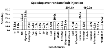
Figure 5. The speedup of using PARIS over random FI to predict the rate of manifestations.

6.2. Efficiency Study–Comparing with Random Fault Injection

We compare the time of using FI and using PARIS to predict the rate of manifestations for the 25 big benchmarks. The number of FIs is determined by using a statistical approach (Leveugle et al., 2009) with the confidence level of 99% and the margin of error 1%. In particular, we use 3000 FIs for each benchmark. When measuring the time of using PARIS, we measure the time spent on the whole workflow, including dynamic instruction trace generation, feature extraction, and making prediction with the trained machine learning model.

Figure 5 shows the results. In general, the speedup of using PARIS over random FI is up to 450x (see LULESH). Among the 25 benchmarks, PARIS is faster than random FI for 20 benchmarks. For one benchmark (LU), PARIS uses almost the same time as FI. For the four benchmarks (CG, BT, SP, and bfs), PARIS is slower, because of the time-consuming trace generation. We hope to improve the performance of the trace generation by using trace compression in the future.

6.3. Feature Selection and Analysis

We use the feature selection technique (i.e., the voting strategy) discussed in Section 4.4 to select features. We analyze the feature selection result in this section.

Table 3 shows the global indexes for all features. Table 3.a reveals that the 4th dimension (the memory-related instructions), 24th dimension (the memory-related instructions in bigram), and 8th dimension (the pattern of overwriting) in $\mathcal{F}^{ave}_{30}$ rank the highest; Table 3.b reveals that the 14th dimension (the memory-related instructions in bigram), 18th dimension (the pattern of overwriting in bigram), and 4th dimension (the memory-related instructions) in $\mathcal{F}^{ave}_{30}$ rank the highest. Those dimensions are the memory-related instructions, which seem to matter most to the application resilience.

In addition, both tables reveal that the 9th dimension (i.e., the pattern of dead location), 19th dimension (i.e., the pattern of dead location in bigram), and 29th dimension (i.e., the pattern of dead location in bigram) rank relatively low. This result indicates that the feature of dead location seems to contribute less to application resilience than the other features.

6.4. Evaluation of Model Tuning and Feature Construction Optimization

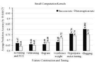
Figure 6. Evaluating the impact of model tuning and feature construction optimization on the prediction accuracy for the three rates. Notation: FCO = “feature construction optimization”.

We study the impact of our model tuning (whitening, bagging and tuning hyperparameters) and feature construction techniques (bigram and resilience weight) on the model accuracy. We use the Gradient Boosting Regression model and 100 small computation kernels (for training) for our study. We start with the model without any of the five techniques, and then apply them one by one.

Figure 6 shows the results. We can see that the prediction accuracy keeps increasing after we apply those techniques one by one. This demonstrates the effectiveness of our techniques. Among the five techniques, the most effective ones are resilience weight, hyperparameters tuning, and bagging when predicting the success rate, and bigram and resilience weight when predicting the interruption rate.

We notice that introducing bigram, the average prediction accuracy is not increased when predicting the success rate. However, examining individual computation kernels, we find that the prediction accuracy for 71% of kernels becomes better, with up to 26% improvement in the prediction accuracy. There are two outliers that largely decrease prediction accuracy after applying bigram. Furthermore, when predicting the interruption rate, the average prediction accuracy increases 3% after applying bigram into features. 3% is a large improvement in the machine learning field. Hence, we conclude that using bigram is very helpful to improve the modeling accuracy.

7. Related Work

Using Machine Learning to Address Resilience Problems. There are a couple of recent efforts that use machine learning  (Mitra et al., 2015; Laguna et al., 2016; Vishnu et al., 2016; Das et al., 2018; Ashraf et al., 2015; Nie et al., 2018) to address resilience problems. Mitra et al. (Mitra et al., 2015) build a regression model to predict anomaly output of an application, given a certain combination of input parameters to the application. Laguna et al. (Laguna et al., 2016) train a machine learning classifier IPAS. IPAS learns which instructions can have a high likelihood of leading to a silent output corruption. IPAS duplicates those instructions to mitigate the effect of silent output corruption. Vishnu et al. (Vishnu et al., 2016) use attributes including system and application states to predict whether a multi-bit error will lead to corrupted output. Desh (Das et al., 2018) predict node failures by training a recurrent neural network model using system logs. Nie et al. (Nie et al., 2018) use system characteristics such as temperature, power consumption, application states as features to predict the occurrence of GPU errors. PARIS is the first work applying machine learning to predict the rate of manifestations.

Random FI. This is the most common method is to study application resilience  (Cher et al., 2014; Calhoun et al., 2014; Kumar Sastry Hari et al., 2017; Li et al., 2012; De Oliveira et al., 2017; Luo et al., 2014; Karlsson et al., 1994; Parasyris et al., 2014; Li et al., 2008; Fang et al., 2014; Kanawati et al., 1995). Typically application-level FI has to be performed many times to ensure statistical significance. Some research prunes unnecessary FI to reduce FI efforts. Hari et al.  (Hari et al., 2012) explore instruction equivalence for selective FI. They further reduce FI positions by leveraging the equivalence of intermediate states in execution and instruction-level approximate computing  (Sastry Hari et al., 2014; Venkatagiri et al., 2016). Our work tries to address the inefficiency of FI to study application resilience. But the above existing work is complementary to our work.

Error Propagation Analysis. Application level error propagation has been widely studied. Li et al. (Li et al., 2016) implement a FI tool to study error propagation in GPU applications, and Trident (Li et al., 2018), a three-level error propagation model to predict SDC probabilities of programs. Calhoun et al. (Calhoun et al., 2017) study how corruption state changes due to error propagation at the instruction and application variable level for three applications. Ashraf et al. (Ashraf et al., 2015) propose an error propagation model to study error propagation for MPI applications. Our work does not focus on error propagation, but includes an N-gram based technique to embed the execution order information into the feature vector to consider the effects of error propagation.

8. Conclusions

As supercomputers increase in size and complexity, the rate of transient faults is expected to increase and becomes a severe problem threatening computation correctness. Techniques to understand the manifestation of transient faults become increasingly important to ensure result correctness for those applications running on supercomputers. This paper introduces PARIS, a machine learning based approach to predict the rate of manifestations of transient faults. We train PARIS on 100 small computation kernels and test on 25 big benchmarks using features highly related to application resilience. We test 18 regression models and find the Gradient Boosting Regression the best machine learning model for predicting the rate of manifestations of transient faults in terms of prediction accuracy.

References

- (1)
- cor (2006) 2006. Coral Benchmark Codes. https://asc.llnl.gov/CORAL-benchmarks/.
- Aktulga et al. (2012) Hasan Metin Aktulga, Joseph C Fogarty, Sagar A Pandit, and Ananth Y Grama. 2012. Parallel reactive molecular dynamics: Numerical methods and algorithmic techniques. Parallel Comput. (2012).
- Ashraf et al. (2015) Rizwan Ashraf, Roberto Gioiosa, Gokcen Kestor, Ronald F. DeMara, Chen-Yong Cher, and Pradip Bose. 2015. Understanding the Propagation of Transient Errors in HPC Applications. In SC.
- Bailey et al. (1992) D. H. Bailey, L. Dagum, E. Barszcz, and H. D. Simon. 1992. NAS Parallel Benchmark Results. In International Conference for High Performance Computing, Networking, Storage and Analysis (SC).
- Baumann (2005) Robert C Baumann. 2005. Radiation-induced soft errors in advanced semiconductor technologies. IEEE Transactions on Device and materials reliability 5, 3 (2005), 305–316.
- Bautista-Gomez et al. (2016) Leonardo Bautista-Gomez, Ferad Zyulkyarov, Osman Unsal, and Simon McIntosh-Smith. 2016. Unprotected computing: A large-scale study of dram raw error rate on a supercomputer. In SC.
- Bergstra and Bengio (2012) James Bergstra and Yoshua Bengio. 2012. Random search for hyper-parameter optimization. Journal of Machine Learning Research (2012).
- Bienia et al. (2008) Christian Bienia, Sanjeev Kumar, Jaswinder Pal Singh, and Kai Li. 2008. The PARSEC benchmark suite: Characterization and architectural implications. In Proceedings of the 17th international conference on Parallel architectures and compilation techniques.
- Brown et al. (1992) Peter F Brown, Peter V Desouza, Robert L Mercer, Vincent J Della Pietra, and Jenifer C Lai. 1992. Class-based n-gram models of natural language. Computational linguistics 18, 4 (1992), 467–479.
- Calhoun et al. (2014) Jon Calhoun, Luke Olson, and Marc Snir. 2014. FlipIt: An LLVM Based Fault Injector for HPC. In Workshops in Euro-Par.
- Calhoun et al. (2017) Jon Calhoun, Marc Snir, Luke N. Olson, and William D. Gropp. 2017. Towards a More Complete Understanding of SDC Propagation. In International Symposium on High-Performance Parallel and Distributed Computing (HPDC).
- Cavnar et al. (1994) William B Cavnar, John M Trenkle, et al. 1994. N-gram-based text categorization. Ann arbor mi 48113, 2 (1994), 161–175.
- Che et al. (2009) S. Che, M. Boyer, J. Meng, D. Tarjan, J. W. Sheaffer, S.-H. Lee, and K. Skadron. 2009. Rodinia: A Benchmark Suite for Heterogeneous Computing. In IEEE International Symposium on Workload Characterization (IISWC).
- Chen et al. (2017) Guobin Chen, Wongun Choi, Xiang Yu, Tony Han, and Manmohan Chandraker. 2017. Learning efficient object detection models with knowledge distillation. In NIPS.
- Chen et al. (2015) Xinchi Chen, Xipeng Qiu, Chenxi Zhu, and Xuanjing Huang. 2015. Gated recursive neural network for chinese word segmentation. In ACL.
- Cher et al. (2014) C.-Y. Cher, M. S. Gupta, P. Bose, and K. P. Muller. 2014. Understanding Soft Error Resiliency of BlueGene/Q Compute Chip Through Hardware Proton Irradiation and Software Fault Injection. In SC.
- Coates et al. (2011) Adam Coates, Andrew Ng, and Honglak Lee. 2011. An analysis of single-layer networks in unsupervised feature learning. In AISTATS.
- Das et al. (2018) Anwesha Das, Frank Mueller, Charles Siegel, and Abhinav Vishnu. 2018. Desh: deep learning for system health prediction of lead times to failure in HPC. In HPDC.
- Das (2001) Sanmay Das. 2001. Filters, wrappers and a boosting-based hybrid for feature selection. In ICML.
- De Oliveira et al. (2017) Daniel Alfonso Goncalves De Oliveira, Laercio Lima Pilla, Mauricio Hanzich, Vinicius Fratin, Fernando Fernandes, Caio Lunardi, José María Cela, Philippe Olivier Alexandre Navaux, Luigi Carro, and Paolo Rech. 2017. Radiation-induced error criticality in modern HPC parallel accelerators. In HPCA.
- Domingos (2000) Pedro Domingos. 2000. Bayesian averaging of classifiers and the overfitting problem. In ICML.
- Domingos and Hulten (2000) Pedro Domingos and Geoff Hulten. 2000. Mining high-speed data streams. In SIGKDD.
- Elliott et al. (2013) James Elliott, Frank Mueller, Miroslav Stoyanov, and Clayton Webster. 2013. Quantifying the impact of single bit flips on floating point arithmetic. In Technical report ORNL/TM-2013/282. Oak Ridge National Laboratory.
- Fang et al. (2014) Bo Fang, Karthik Pattabiraman, Matei Ripeanu, and Sudhanva Gurumurthi. 2014. Gpu-qin: A methodology for evaluating the error resilience of gpgpu applications. In ISPASS.
- Georgakoudis et al. (2017) Giorgis Georgakoudis, Ignacio Laguna, Dimitrios S. Nikolopoulos, and Martin Schulz. 2017. REFINE : Realistic Fault Injection via Compiler-based Instrumentation for Accuracy , Portability and Speed. In SC.
- Guo et al. (2018) Luanzheng Guo, Dong Li, Ignacio Laguna, and Schulz Martin. 2018. FlipTracker: Understanding Natural Error Resilience in HPC Applications. arXiv preprint arXiv:1809.01362 (2018).
- HackerRank (2009) HackerRank. 2009. HackerRank Home Page. https://www.hackerrank.com/.
- Hari et al. (2012) Siva Kumar Sastry Hari, Sarita V. Adve, Helia Naeimi, and Pradeep Ramachandran. 2012. Relyzer: Exploiting Application-level Fault Equivalence to Analyze App. Resiliency to Transient Faults. In ASPLOS.
- Henning (2000) John L Henning. 2000. SPEC CPU2000: Measuring CPU performance in the new millennium. Computer (2000).
- Kaliorakis et al. (2017) Manolis Kaliorakis, Dimitris Gizopoulos, Ramon Canal, and Antonio Gonzalez. 2017. MeRLiN: Exploiting Dynamic Instruction Behavior for Fast and Accurate Microarchitecture Level Reliability Assessment. In ISCA.
- Kanawati et al. (1995) Ghani A. Kanawati, Nasser A. Kanawati, and Jacob A. Abraham. 1995. FERRARI: A flexible software-based fault and error injection system. IEEE Transactions on computers (1995).
- Karlsson et al. (1994) Johan Karlsson, Peter Liden, Peter Dahlgren, Rolf Johansson, and Ulf Gunneflo. 1994. Using heavy-ion radiation to validate fault-handling mechanisms. IEEE micro (1994).
- Kohavi (1995) Ron Kohavi. 1995. A study of cross-validation and bootstrap for accuracy estimation and model selection. In IJCAI.
- Kumar Sastry Hari et al. (2017) Siva Kumar Sastry Hari, Timothy Tsai, Mark Stephenson, Stephen W. Keckler, and Joel Emer. 2017. SASSIFI: An architecture-level fault injection tool for GPU application resilience evaluation. In ISPASS.
- Laguna et al. (2016) Ignacio Laguna, Martin Schulz, David F Richards, Jon Calhoun, and Luke Olson. 2016. IPAS: Intelligent protection against silent output corruption in scientific applications. In CGO.
- Lattner and Adve (2004) Chris Lattner and Vikram Adve. 2004. LLVM: A compilation framework for lifelong program analysis & transformation. In Proceedings of the international symposium on Code generation and optimization: feedback-directed and runtime optimization (CGO).
- Leveugle et al. (2009) Régis Leveugle, A Calvez, Paolo Maistri, and Pierre Vanhauwaert. 2009. Statistical fault injection: Quantified error and confidence. In Proceedings of the Conference on Design, Automation and Test in Europe. European Design and Automation Association, 502–506.
- Li et al. (2012) Dong Li, Jeffrey S. Vetter, and Weikuan Yu. 2012. Classifying Soft Error Vulnerabilities in Extreme-Scale Scientific Applications Using a Binary Instrumentation Tool. In International Conference for High Performance Computing, Networking, Storage and Analysis (SC).
- Li et al. (2016) Guanpeng Li, Karthik Pattabiraman, Chen-Yong Cher, and Pradip Bose. 2016. Understanding Error Propagation in GPGPU. In Proceedings of the International Conference for High Performance Computing, Networking, Storage and Analysis (SC).
- Li et al. (2018) Guanpeng Li, Karthik Pattabiraman, Siva Kumar Sastry Hari, Michael Sullivan, and Timothy Tsai. 2018. Modeling Soft-Error Propagation in Programs. In DSN.
- Li et al. (2008) Man-Lap Li, Pradeep Ramachandran, Swarup Kumar Sahoo, Sarita V Adve, Vikram S Adve, and Yuanyuan Zhou. 2008. Understanding the Propagation of Hard Errors to Software and Implications for Resilient System Design. In ASPLOS.
- Liu et al. (2016) Mingxia Liu, Daoqiang Zhang, Ehsan Adeli, and Dinggang Shen. 2016. Inherent Structure-Based Multiview Learning With Multitemplate Feature Representation for Alzheimer’s Disease Diagnosis. IEEE Trans. Biomed. Engineering 63, 7 (2016), 1473–1482.
- Luo et al. (2014) Yixin Luo, Sriram Govindan, Bikash Sharma, Mark Santaniello, Justin Meza, Aman Kansal, Jie Liu, Badriddine Khessib, Kushagra Vaid, and Onur Mutlu. 2014. Characterizing application memory error vulnerability to optimize datacenter cost via heterogeneous-reliability memory. In DSN.
- Menon and Mohror (2018) Harshitha Menon and Kathryn Mohror. 2018. DisCVar: discovering critical variables using algorithmic differentiation for transient faults. In PPOPP.
- Mitra et al. (2015) Subrata Mitra, Greg Bronevetsky, Suhas Javagal, and Saurabh Bagchi. 2015. Dealing with the unknown: Resilience to prediction errors. In PACT.
- Nie et al. (2018) Bin Nie, Ji Xue, Saurabh Gupta, Tirthak Patel, Christian Engelmann, Evgenia Smirni, and Devesh Tiwari. 2018. Machine Learning Models for GPU Error Prediction in a Large Scale HPC System. In DSN.
- Parasyris et al. (2014) Konstantinos Parasyris, Georgios Tziantzoulis, Christos D Antonopoulos, and Nikolaos Bellas. 2014. GemFI: A fault injection tool for studying the behavior of applications on unreliable substrates. In DSN.
- Pedregosa et al. (2011) F. Pedregosa, G. Varoquaux, A. Gramfort, V. Michel, B. Thirion, O. Grisel, M. Blondel, P. Prettenhofer, R. Weiss, V. Dubourg, J. Vanderplas, A. Passos, D. Cournapeau, M. Brucher, M. Perrot, and E. Duchesnay. 2011. Scikit-learn: Machine Learning in Python. Journal of Machine Learning Research 12 (2011), 2825–2830.
- Pei et al. (2014) Wenzhe Pei, Tao Ge, and Baobao Chang. 2014. Max-margin tensor neural network for chinese word segmentation. In ACL.
- Sangchoolie et al. (2017) Behrooz Sangchoolie, Karthik Pattabiraman, and Johan Karlsson. 2017. One Bit is (Not) Enough: An Empirical Study of the Impact of Single and Multiple Bit-Flip Errors. In DSN.
- Sastry Hari et al. (2014) Siva Kumar Sastry Hari, Radha Venkatagiri, Sarita V. Adve, and Helia Naeimi. 2014. GangES: Gang Error Simulation for Hardware Resiliency Evaluation. In International Symposium on Computer Arch.
- Shao and Brooks (2013) Yakun Sophia Shao and David Brooks. 2013. ISA-Independent Workload Characterization and its Implications for Specialized Architectures. In ISPASS.
- Sridharan et al. (2015) Vilas Sridharan, Nathan DeBardeleben, Sean Blanchard, Kurt B. Ferreira, and Sudhanva Gurumurthi. 2015. Mem Errors in Modern Systems: The Good, The Bad, and The Ugly. In ASPLOS.
- Taborda and Bielak (2011) Ricardo Taborda and Jacobo Bielak. 2011. Large-scale earthquake simulation: computational seismology and complex engineering systems. Computing in Science & Engineering (2011).
- Thomas and Pattabiraman (2013) Anna Thomas and Karthik Pattabiraman. 2013. LLFI: An intermediate code level fault injector for soft computing applications. In SELSE.
- Tsymbal et al. (2005) Alexey Tsymbal, Mykola Pechenizkiy, and Pádraig Cunningham. 2005. Diversity in search strategies for ensemble feature selection. Information fusion 6, 1 (2005), 83–98.
- Venkatagiri et al. (2016) R. Venkatagiri, A. Mahmoud, S. K. S. Hari, and S. V. Adve. 2016. Approxilyzer: Towards a systematic framework for instruction-level approximate computing and its application to hardware resiliency. In MICRO.
- Vishnu et al. (2016) Abhinav Vishnu, Hubertus van Dam, Nathan R Tallent, Darren J Kerbyson, and Adolfy Hoisie. 2016. Fault modeling of extreme scale applications using machine learning. In IPDPS.
- Wei et al. (2014) Jiesheng Wei, Anna Thomas, Guanpeng Li, and Karthik Pattabiraman. 2014. Quantifying the Accuracy of High-Level Fault Injection Techniques for Hardware Faults. In DSN.
- Xu and Li (2012) Xin Xu and Man-Lap Li. 2012. Understanding Soft Error Propagation Using Vulnerability-driven Fault Injection. In DSN.
- Zhang et al. (2006) Xuegong Zhang, Xin Lu, Qian Shi, Xiu-qin Xu, E Leung Hon-chiu, Lyndsay N Harris, James D Iglehart, Alexander Miron, Jun S Liu, and Wing H Wong. 2006. Recursive SVM feature selection and sample classification for mass-spectrometry and microarray data. BMC bioinformatics 7, 1 (2006), 197.