When Bifidelity Meets CoKriging: An Efficient Physics-Informed Multifidelity Method

Abstract

In this work, we propose a framework that combines the approximation-theory-based multifidelity method and Gaussian-process-regression-based multifidelity method to achieve data-model convergence when stochastic simulation models and sparse accurate observation data are available. Specifically, the two types of multifidelity methods we use are the bifidelity and CoKriging methods. The new approach uses the bifidelity method to efficiently estimate the empirical mean and covariance of the stochastic simulation outputs, then it uses these statistics to construct a Gaussian process (GP) representing low-fidelity in CoKriging. We also combine the bifidelity method with Kriging, where the approximated empirical statistics are used to construct the GP as well. We prove that the resulting posterior mean by the new physics-informed approach preserves linear physical constraints up to an error bound. By using this method, we can obtain an accurate construction of a state of interest based on a partially correct physical model and a few accurate observations. We present numerical examples to demonstrate performance of the method.

Keywords: physics-informed, Gaussian process regression, CoKriging, multifidelity, bifidelity, error bound.

1 Introduction

Gaussian process (GP), a widely used tool in statistics, and machine learning  [7, 37, 40], has become popular in probabilistic scientific computing. GP regression (GPR), also known as Kriging in geostatistics, constructs a statistical model of a partially observed process by assuming that its observations are a realization of a GP. A GP is uniquely described by its mean and covariance function (also known as kernel). Its variant, CoKriging, was originally formulated to compute predictions of sparsely observed states of physical systems by leveraging observations of other states or parameters of the system [39, 19]. Recently, it has been employed for constructing multi-fidelity models [17, 23, 33], and has been applied in various fields, e.g., [22, 1, 30]. In the widely used stationary Kriging/CoKriging method, usually parameterized forms of mean and covariance functions are assumed, and the hyperparameters of these functions (e.g., variance and correlation length) are estimated by maximizing the log marginal likelihood of the data.

Recently a new framework, physics-informed Kriging (PhIK)/physics-informed CoKriging (CoPhIK), was developed for those applications where partially correct physical models along with sparse observation data are available [49, 46]. These physical models are constructed based on domain knowledge, and they include random variables or random fields to represent the lack of knowledge (e.g., unknown physical law, uncertain parameters, etc). The PhIK/CoPhIK framework combines the realizations of the stochastic physical model with the observation data to provide an accurate reconstruct of the state of interest on the entire computational domain. These realizations are then used to approximate mean and covariance in the PhIK/CoPhIK framework. The most popular approach of obtaining model realizations is the Monte Carlo (MC) simulation, and it can be replaced by more efficient approaches to estimate mean and covariance, e.g., quasi-Monte Carlo [29], probabilistic collocation [42, 45], Analysis Of Variance (ANOVA) [25, 47], compressive sensing [4, 48], and the moment equation method [41].

It is worthy to note that the aforementioned approaches rely on single a fidelity solver. For large scale applications, the computational cost can still be prohibitive if a large number of samples are required. In many practical problems, low-fidelity models for the underlying problem are often available, and it is much less expensive to obtain the realizations of these models. Even though their accuracy is not high, they can still capture some important physics of the underlying models with low computational cost. Therefore, it is highly desirable to utilize the computational efficiency of low-fidelity models to reduce the overall computational cost. Many multifidelity algorithms have been developed based on different principles in different contexts. These include (a) multi-level Monte Carlo (MLMC) [10, 2], which is already used in PhIK and CoPhIK to reduce the computational cost [49, 46]; (b) meta-models through GP, i.e., CoKriging [17, 43, 34]; (c) variance reduced based approaches, i.e., control-variate based approach [32], importance sampling [31]; and (d) model discrepancy based approaches [28, 5]. Another trend in the context of uncertainty quantification is to explore the parameter space by using a large number of low-fidelity samples to identify a small set of important basis, then learn the “best” approximation rule of the target high-fidelity solution or its statistics based on the selected basis [27, 51, 50, 6]. Previous works demonstrated its potential to significantly reduce the computational cost for various applications by utilizing $\mathcal{O}(10)$ high-fidelity simulations, including combustion modeling [26], orbit-state uncertainty propagation [15], molecular dynamics simulations [36], and turbulence modeling [14], to name a few.

In this work, we propose to employ the multifidelity approaches presented in [27, 51] to accelerate the computation of PhIK and CoPhIK. For demonstration purpose, we consider the bifidelity model in this work, and the proposed framework can be implemented in multifidelity (more than two fidelity) models.

2 Methodology

In this section, we begin by reviewing the general GPR framework [44], the Kriging and CoKriging methods with stationary kernel [7], the PhIK [49] and CoPhIK [46] methods, and the bi-fidelity approach [51]. Then, we introduce the bi-fidelity-aided PhIK and CoPhIK methods.

2.1 GPR framework

We denote the observation locations as $\bm{X}=\{\bm{x}^{(i)}\}_{i=1}^{N}$ ($\bm{x}^{(i)}$ are $d$-dimensional vectors in $D\subseteq\mathbb{R}^{d}$) and the observed state values at these locations as $\bm{y}=(y^{(1)},y^{(2)},\dotsc,y^{(N)})^{\top}$ ($y^{(i)}\in\mathbb{R}$). For simplicity, we assume that $y^{(i)}$ are scalars. We aim to predict $y$ at any new location $\bm{x}^{*}\in D$. The GPR method assumes that the observation vector $\bm{y}$ is a realization of the following $N$-dimensional random vector that satisfies multivariate Gaussian distribution:

$$\bm{Y}=\left(Y(\bm{x}^{(1)}),Y(\bm{x}^{(2)}),\dotsc,Y(\bm{x}^{(N)})\right)^{\top},$$

where $Y(\bm{x}^{(i)})$ is the concise notation of $Y(\bm{x}^{(i)};\omega)$, and $Y(\bm{x}^{(i)};\omega)$ is a Gaussian random variable defined on a probability space $(\Omega,\mathcal{F},P)$ with $\omega\in\Omega$. Of note, $\bm{x}^{(i)}$ can be considered as parameters for the GP $Y(\cdot,\cdot):D\times\Omega\rightarrow\mathbb{R}$, such that $Y(\bm{x}^{(i)},\cdot):\Omega\rightarrow\mathbb{R}$ is a Gaussian random variable for any $\bm{x}^{(i)}$ in the set $D$. Usually, the GP $Y(\bm{x})$ is denoted as

$$Y(\bm{x})\sim\mathcal{GP}\left(\mu(\bm{x}),k(\bm{x},\bm{x}^{\prime})\right),$$ (2.1)

where $\mu(\cdot):D\rightarrow\mathbb{R}$ and $k(\cdot,\cdot):D\times D\rightarrow\mathbb{R}$ are the mean and covariance functions:

$$\mu(\bm{x}) =\mathbb{E}\left\{Y(\bm{x})\right\},$$ (2.2)

$$k(\bm{x},\bm{x}^{\prime}) =\text{Cov}\left\{Y(\bm{x}),Y(\bm{x}^{\prime})\right\}=\mathbb{E}\left\{(Y(\bm{x})-\mu(\bm{x}))(Y(\bm{x}^{\prime})-\mu(\bm{x}^{\prime}))\right\}.$$ (2.3)

The variance of $Y(\bm{x})$ is $k(\bm{x},\bm{x})$, and its standard deviation is $\sigma(\bm{x})=\sqrt{k(\bm{x},\bm{x})}$. The covariance matrix of random vector $\bm{Y}$, denoted as $\mathbf{C}$, is defined as $C_{ij}=k(\bm{x}^{(i)},\bm{x}^{(j)})$. Functions $\mu(\bm{x})$ and $k(\bm{x},\bm{x}^{\prime})$ are obtained by identifying their hyperparameters via maximizing the log marginal likelihood [44]:

$$\ln L=-\dfrac{1}{2}(\bm{y}-\bm{\mu})^{\top}\mathbf{C}^{-1}(\bm{y}-\bm{\mu})-\dfrac{1}{2}\ln|\mathbf{C}|-\dfrac{N}{2}\ln 2\pi,$$ (2.4)

where $\bm{\mu}=(\mu(\bm{x}^{(1)}),\dotsc,\bm{x}^{(N)})^{\top}$. The result of GPR is a posterior distribution $y(\bm{x}^{*})\sim\mathcal{N}(\hat{y}(\bm{x}^{*}),\hat{s}^{2}(\bm{x}^{*}))$ for any $\bm{x}^{*}\in D$, where

$$\hat{y}(\bm{x}^{*}) =\mu(\bm{x}^{*})+\bm{c}(\bm{x}^{*})^{\top}\mathbf{C}^{-1}(\bm{y}-\bm{\mu}),$$ (2.5)

$$\hat{s}^{2}(\bm{x}^{*}) =\sigma^{2}(\bm{x}^{*})-\bm{c}(\bm{x}^{*})^{\top}\mathbf{C}^{-1}\bm{c}(\bm{x}^{*}),$$ (2.6)

and $\bm{c}(\bm{x}^{*})$ is a vector of covariance, i.e., $(\bm{c}(\bm{x}^{*}))_{i}=k(\bm{x}^{(i)},\bm{x}^{*})$. In practice, it is common to use $\hat{y}(\bm{x}^{*})$ as the prediction, and $\hat{s}^{2}(\bm{x}^{*})$ is also called the mean squared error (MSE) of the prediction because $\hat{s}^{2}(\bm{x}^{*})=\mathbb{E}\left\{(\hat{y}(\bm{x}^{*})-Y(\bm{x}^{*}))^{2}\right\}$ [7]. Consequently, $\hat{s}(\bm{x}^{*})$ is the root mean squared error (RMSE). Moreover, to account for the observation noise, one can assume that the noise is independent and identically distributed (i.i.d.) Gaussian random variables with zero mean and variance $\delta^{2}$, and replace $\mathbf{C}$ with $\mathbf{C}+\delta^{2}\mathbf{I}$. In this study, we assume that observations $\bm{y}$ are noiseless. If $\mathbf{C}$ is not invertible or its condition number is very large, one can add a small regularization term $\alpha\mathbf{I}$ ($\alpha$ is a small positive real number) to $\mathbf{C}$, which is equivalent to assuming there is an observation noise. In addition, $\hat{s}$ can be used in global optimization, or in the greedy algorithm to identify locations of additional observations. Specifically, in the greedy algorithm, the new observations can be added at the maxima of $\hat{s}$, see Appendix A for details.

2.2 Kriging and CoKriging with stationary kernel

In the widely used ordinary Kriging method, a stationary GP is assumed [18]. Specifically, $\mu$ is set as a constant $\mu(\bm{x})\equiv\mu$, and $k(\bm{x},\bm{x}^{\prime})=k(\bm{\tau})$, where $\bm{\tau}=\bm{x}-\bm{x}^{\prime}$. Consequently, $\sigma^{2}(\bm{x})=k(\bm{x},\bm{x})=k(\bm{0})=\sigma^{2}$ is a constant. Popular forms of kernels include polynomial, exponential, Gaussian (squared-exponential), and Matérn functions. For example, the Gaussian kernel can be written as $k(\bm{\tau})=\sigma^{2}\exp\left(-\frac{1}{2}\|\bm{x}-\bm{x}^{\prime}\|^{2}_{w}\right)$, where the weighted norm is defined as $\displaystyle\|\bm{x}-\bm{x}^{\prime}\|^{2}_{w}=\sum_{i=1}^{d}\left(\dfrac{x_{i}-x^{\prime}_{i}}{l_{i}}\right)^{2}$. Here, $l_{i}$ ($i=1,\dotsc,d$), the correlation lengths of $\bm{y}$ in the $i$ direction, are constants. Given a stationary covariance function, the covariance matrix $\mathbf{C}$ of $\bm{Y}$ can be written as $\mathbf{C}=\sigma^{2}\mathbf{\Psi}$, where $\Psi_{ij}=\exp(-\frac{1}{2}\|\bm{x}^{(i)}-\bm{x}^{(j)}\|_{w}^{2})$. In the MLE framework, the estimators of $\mu$ and $\sigma^{2}$, denoted as $\hat{\mu}$ and $\hat{\sigma}^{2}$, are

$$\hat{\mu}=\dfrac{\bm{1}^{\top}\mathbf{\Psi}^{-1}\bm{y}}{\bm{1}^{\top}\mathbf{\Psi}^{-1}\bm{1}},\qquad\hat{\sigma}^{2}=\dfrac{(\bm{y}-\bm{1}\hat{\mu})^{\top}\mathbf{\Psi}^{-1}(\bm{y}-\bm{1}\hat{\mu})}{N},$$ (2.7)

where $\bm{1}$ is a constant vector consisting of $1$ [7]. The hyperparameters $\sigma$ and $l_{i}$ are estimated by maximizing the log marginal likelihood in Eq. (2.4). The $\hat{y}(\bm{x}^{*})$ and $\hat{s}^{2}(\bm{x}^{*})$ in Eq. (2.5) take the following form:

$$\hat{y}(\bm{x}^{*}) =\hat{\mu}+\bm{\psi}^{\top}\mathbf{\Psi}^{-1}(\bm{y}-\bm{1}\hat{\mu}),$$ (2.8)

$$\hat{s}^{2}(\bm{x}^{*}) =\hat{\sigma}^{2}\left(1-\psi^{\top}\mathbf{\Psi}^{-1}\bm{\psi}\right),$$ (2.9)

where $\bm{\psi}=\bm{\psi}(\bm{x}^{*})$ is a vector of correlations between the observed data and the prediction, i.e., $\psi_{i}=\frac{1}{\sigma^{2}}k(\bm{x}^{(i)},\bm{x}^{*})$.

Next, we briefly review the formulation of CoKriging for two-level multifidelity modeling. Suppose that we have high-fidelity data (e.g., accurate measurements of states) $\bm{y}_{H}=\left(y_{H}^{(1)},\dotsc,y_{H}^{(N_{H})}\right)^{\top}$ at locations $\bm{X}_{H}=\left\{\bm{x}_{H}^{(i)}\right\}_{i=1}^{N_{H}}$, and low-fidelity data (e.g., simulation results) $\bm{y}_{L}=\left(y_{L}^{(1)},\dotsc,y_{L}^{(N_{L})}\right)^{\top}$ at locations $\bm{X}_{L}=\left\{\bm{x}_{L}^{(i)}\right\}_{i=1}^{N_{L}}$, where $y_{H}^{(i)},y_{L}^{(i)}\in\mathbb{R}$ and $\bm{x}_{H}^{(i)},\bm{x}_{L}^{(i)}\in D\subseteq\mathbb{R}^{d}$. We denote $\mathclap{\phantom{\bm{X}}\mathclap{\widetilde{\mathclap{\phantom{X}\mathclap{\bm{X}\,}}\phantom{X}}}}\phantom{\bm{X}}=\{\bm{X}_{L},\bm{X}_{H}\}$ and $\mathclap{\phantom{\bm{y}}\mathclap{\widetilde{\mathclap{\phantom{y}\mathclap{\bm{y}\,}}\phantom{y}}}}\phantom{\bm{y}}=\left(\bm{y}_{L}^{\top},\bm{y}_{H}^{\top}\right)^{\top}$.

Kennedy and O’Hagan [17] proposed a multifidelity formulation based on the auto-regressive model for GP $Y_{H}$ ($\sim\mathcal{GP}(\mu_{H}(\cdot),k_{H}(\cdot,\cdot))$):

$$Y_{H}(\bm{x})=\rho Y_{L}(\bm{x})+Y_{d}(\bm{x}),$$ (2.10)

where $Y_{L}(\cdot)$ ($\sim\mathcal{GP}(\mu_{L}(\cdot),k_{L}(\cdot,\cdot))$) regresses the low-fidelity data, $\rho\in\mathbb{R}$ is a regression parameter and $Y_{d}(\cdot)$ ($\sim\mathcal{GP}(\mu_{d}(\cdot),k_{d}(\cdot,\cdot))$ models the difference between $Y_{H}$ and $\rho Y_{L}$. This model assumes that

$$\text{Cov}\left\{Y_{H}(\bm{x}),Y_{L}({\bm{x}}^{\prime})\mid Y_{L}(\bm{x})\right\}=0,\quad\text{for all}\quad\bm{x}^{\prime}\neq\bm{x},\ \bm{x},\bm{x}^{\prime}\in D.$$ (2.11)

The covariance of observations, $\mathclap{\phantom{\mathbf{C}}\mathclap{\widetilde{\mathclap{\phantom{C}\mathclap{\mathbf{C}\,}}\phantom{C}}}}\phantom{\mathbf{C}}$, is then given by

$$\mathclap{\phantom{\mathbf{C}}\mathclap{\widetilde{\mathclap{\phantom{C}\mathclap{\mathbf{C}\,}}\phantom{C}}}}\phantom{\mathbf{C}}=\begin{pmatrix}\mathbf{C}_{L}(\bm{X}_{L},\bm{X}_{L})&\rho\mathbf{C}_{L}(\bm{X}_{L},\bm{X}_{H})\\ \rho\mathbf{C}_{L}(\bm{X}_{H},\bm{X}_{L})&\rho^{2}\mathbf{C}_{L}(\bm{X}_{H},\bm{X}_{H})+\mathbf{C}_{d}(\bm{X}_{H},\bm{X}_{H})\end{pmatrix},$$ (2.12)

where $\mathbf{C}_{L}$ and $\mathbf{C}_{d}$ are the covariance matrices computed from $k_{L}(\cdot,\cdot)$ and $k_{d}(\cdot,\cdot)$, respectively. One can assume parameterized forms for these kernels (e.g., Gaussian kernel) and employ the following two-step approach [8, 7] to identify hyperparameters:

1. Use Kriging to construct $Y_{L}$ using $\{\bm{X}_{L},\bm{y}_{L}\}$.

2. Denote $\bm{y}_{d}=\bm{y}_{H}-\rho\bm{y}_{L}(\bm{X}_{H})$, where $\bm{y}_{L}(\bm{X}_{H})$ are the values of $\bm{y}_{L}$ at locations common to those of $\bm{X}_{H}$, then construct $Y_{d}$ using $\{\bm{X}_{H},\bm{y}_{d}\}$ via Kriging.

The posterior mean and variance of $Y_{H}$ at $\bm{x}^{*}\in D$ are given by

$$\hat{y}(\bm{x}^{*}) =\mu_{H}(\bm{x}^{*})+\mathclap{\phantom{\bm{c}}\mathclap{\widetilde{\mathclap{\phantom{y}\mathclap{\bm{c}\,}}\phantom{y}}}}\phantom{\bm{c}}(\bm{x}^{*})^{\top}\mathclap{\phantom{\mathbf{C}}\mathclap{\widetilde{\mathclap{\phantom{C}\mathclap{\mathbf{C}\,}}\phantom{C}}}}\phantom{\mathbf{C}}^{-1}(\mathclap{\phantom{\bm{y}}\mathclap{\widetilde{\mathclap{\phantom{y}\mathclap{\bm{y}\,}}\phantom{y}}}}\phantom{\bm{y}}-\mathclap{\phantom{\bm{\mu}}\mathclap{\widetilde{\mathclap{\phantom{y}\mathclap{\bm{\mu}\,}}\phantom{y}}}}\phantom{\bm{\mu}}),$$ (2.13)

$$\hat{s}^{2}(\bm{x}^{*}) =\rho^{2}\sigma^{2}_{L}(\bm{x}^{*})+\sigma^{2}_{d}(\bm{x}^{*})-\mathclap{\phantom{\bm{c}}\mathclap{\widetilde{\mathclap{\phantom{y}\mathclap{\bm{c}\,}}\phantom{y}}}}\phantom{\bm{c}}(\bm{x}^{*})^{\top}\mathclap{\phantom{\mathbf{C}}\mathclap{\widetilde{\mathclap{\phantom{C}\mathclap{\mathbf{C}\,}}\phantom{C}}}}\phantom{\mathbf{C}}^{-1}\mathclap{\phantom{\bm{c}}\mathclap{\widetilde{\mathclap{\phantom{y}\mathclap{\bm{c}\,}}\phantom{y}}}}\phantom{\bm{c}}(\bm{x}^{*}),$$ (2.14)

where $\mu_{H}(\bm{x}^{*})=\rho\mu_{L}(\bm{x}^{*})+\mu_{d}(\bm{x}^{*})$, $\sigma^{2}_{L}(\bm{x}^{*})=k_{{}_{L}}(\bm{x}^{*},\bm{x}^{*})$, $\sigma^{2}_{d}(\bm{x}^{*})=k_{d}(\bm{x}^{*},\bm{x}^{*})$, and

$$\mathclap{\phantom{\bm{\mu}}\mathclap{\widetilde{\mathclap{\phantom{y}\mathclap{\bm{\mu}\,}}\phantom{y}}}}\phantom{\bm{\mu}} =\begin{pmatrix}\bm{\mu}_{L}\\ \bm{\mu}_{H}\end{pmatrix}=\begin{pmatrix}\big{(}\mu_{L}(\bm{x}_{{}_{L}}^{(1)})\dotsc,\mu_{L}(\bm{x}_{{}_{L}}^{(N_{L})})\big{)}^{\top}\\ \big{(}\mu_{H}(\bm{x}_{{}_{H}}^{(1)})\dotsc,\mu_{H}(\bm{x}_{{}_{H}}^{(N_{H})})\big{)}^{\top}\end{pmatrix},$$ (2.15)

$$\mathclap{\phantom{\bm{c}}\mathclap{\widetilde{\mathclap{\phantom{y}\mathclap{\bm{c}\,}}\phantom{y}}}}\phantom{\bm{c}}(\bm{x}^{*}) =\begin{pmatrix}\rho\bm{c}_{L}(\bm{x}^{*})\\ \bm{c}_{H}(\bm{x}^{*})\end{pmatrix}=\begin{pmatrix}\big{(}\rho k_{L}(\bm{x}^{*},\bm{x}_{L}^{(1)}),\dotsc,\rho k_{{}_{L}}(\bm{x}^{*},\bm{x}_{L}^{(N_{L})})\big{)}^{\top}\\ \big{(}k_{H}(\bm{x}^{*},\bm{x}_{H}^{(1)}),\dotsc,k_{H}(\bm{x}^{*},\bm{x}_{H}^{(N_{H})})\big{)}^{\top}\end{pmatrix},$$ (2.16)

where $k_{H}(\bm{x},\bm{x}^{\prime})=\rho^{2}k_{L}(\bm{x},\bm{x}^{\prime})+k_{d}(\bm{x},\bm{x}^{\prime})$. Here, we have neglected a small contribution to $\hat{s}^{2}$ (see [7]). Alternatively, one can simultaneously identify hyperparameters in $k_{L}(\cdot,\cdot)$ and $k_{d}(\cdot,\cdot)$ along with $\rho$ by maximizing the following log marginal likelihood:

$$\ln\mathclap{\phantom{L}\mathclap{\widetilde{\mathclap{\phantom{I}\mathclap{L\,}}\phantom{I}}}}\phantom{L}=-\dfrac{1}{2}(\mathclap{\phantom{\bm{y}}\mathclap{\widetilde{\mathclap{\phantom{y}\mathclap{\bm{y}\,}}\phantom{y}}}}\phantom{\bm{y}}-\mathclap{\phantom{\bm{\mu}}\mathclap{\widetilde{\mathclap{\phantom{y}\mathclap{\bm{\mu}\,}}\phantom{y}}}}\phantom{\bm{\mu}})^{\top}\mathclap{\phantom{\mathbf{C}}\mathclap{\widetilde{\mathclap{\phantom{C}\mathclap{\mathbf{C}\,}}\phantom{C}}}}\phantom{\mathbf{C}}^{-1}(\mathclap{\phantom{\bm{y}}\mathclap{\widetilde{\mathclap{\phantom{y}\mathclap{\bm{y}\,}}\phantom{y}}}}\phantom{\bm{y}}-\mathclap{\phantom{\bm{\mu}}\mathclap{\widetilde{\mathclap{\phantom{y}\mathclap{\bm{\mu}\,}}\phantom{y}}}}\phantom{\bm{\mu}})-\dfrac{1}{2}\ln\big{|}\mathclap{\phantom{\mathbf{C}}\mathclap{\widetilde{\mathclap{\phantom{C}\mathclap{\mathbf{C}\,}}\phantom{C}}}}\phantom{\mathbf{C}}\big{|}-\dfrac{N_{H}+N_{L}}{2}\ln 2\pi.$$ (2.17)

2.3 PhIK and CoPhIK

The recently proposed PhIK method [49] takes advantage of the existing domain knowledge, e.g., approximate numerical or analytical physics-based models, in the form of realizations of a stochastic model of the system. Consequently, the mean and covariance of the GP model can be approximated using these realizations. As such, there is no need to assume a specific form of the correlation functions and solve an optimization problem for the hyperparameters. These stochastic models typically include random parameters or random processes/fields to reflect the lack of understanding (of physical laws) or knowledge (of the coefficients, parameters, etc.) of the real system. Then, MC simulations can be conducted to generate an ensemble of the state of interest, from which the statistics, e.g., mean and standard deviation, are estimated.

Specifically, assume that we have $M$ realizations of a stochastic model $u(\bm{x};\omega)$ ($\bm{x}\in D,\omega\in\Omega$) denoted as $\{u^{m}(\bm{x})\}_{m=1}^{M}$, and we can build the following GP model:

$$Y(\bm{x})\sim\mathcal{GP}(\mu_{\mathrm{MC}}(\bm{x}),k_{\mathrm{MC}}(\bm{x},\bm{x}^{\prime})),$$ (2.18)

where

$$\mu(\bm{x}) \approx\mu_{\mathrm{MC}}(\bm{x})=\dfrac{1}{M}\sum_{m=1}^{M}u^{m}(\bm{x}),$$ (2.19)

$$k(\bm{x},\bm{x}^{\prime}) \approx k_{\mathrm{MC}}(\bm{x},\bm{x}^{\prime})=\dfrac{1}{M-1}\sum_{m=1}^{M}\left(u^{m}(\bm{x})-\mu_{\mathrm{MC}}(\bm{x})\right)\left(u^{m}(\bm{x}^{\prime})-\mu_{\mathrm{MC}}(\bm{x}^{\prime})\right).$$

Thus, the covariance matrix of $\bm{Y}$ can be estimated as

$$\mathbf{C}\approx\mathbf{C}_{\mathrm{MC}}=\dfrac{1}{M-1}\sum_{m=1}^{M}\left(\bm{u}^{m}-\bm{\mu}_{\mathrm{MC}}\right)\left(\bm{u}^{m}-\bm{\mu}_{\mathrm{MC}}\right)^{\top},$$ (2.20)

where $\bm{u}^{m}=\left(u^{m}(\bm{x}^{(1)}),\dotsc,u^{m}(\bm{x}^{(N)})\right)^{\top}$, $\bm{\mu}_{\mathrm{MC}}=\left(\mu_{\mathrm{MC}}(\bm{x}^{(1)}),\dotsc,\mu_{\mathrm{MC}}(\bm{x}^{(N)})\right)^{\top}$. The prediction and MSE at location $\bm{x}^{*}\in D$ are

$$\hat{y}(\bm{x}^{*}) =\mu_{\mathrm{MC}}(\bm{x}^{*})+\bm{c}_{\mathrm{MC}}(\bm{x}^{*})^{\top}\mathbf{C}_{\mathrm{MC}}^{-1}(\bm{y}-\bm{\mu}_{\mathrm{MC}}),$$ (2.21)

$$\hat{s}^{2}(\bm{x}^{*}) =\hat{\sigma}_{\mathrm{MC}}^{2}(\bm{x}^{*})-\bm{c}_{\mathrm{MC}}(\bm{x}^{*})^{\top}\mathbf{C}_{\mathrm{MC}}^{-1}\bm{c}_{\mathrm{MC}}(\bm{x}^{*}),$$ (2.22)

where $\hat{\sigma}^{2}_{\mathrm{MC}}(\bm{x}^{*})=k_{\mathrm{MC}}(\bm{x}^{*},\bm{x}^{*})$ is the variance of data set $\{u^{m}(\bm{x}^{*})\}_{m=1}^{M}$, and
$\bm{c}_{\mathrm{MC}}(\bm{x}^{*})=\left(k_{\mathrm{MC}}(\bm{x}^{(1)},\bm{x}^{*}),\dotsc,k_{\mathrm{MC}}(\bm{x}^{(N)},\bm{x}^{*})\right)^{\top}$.

Similarly, the CoPhIK method uses model realizations to construct $Y_{L}$ in CoKriging. Specifically, we set $\bm{X}_{L}=\bm{X}_{H}$ to simplify the formula and computing, and denote $N=N_{H}=N_{L}$. We set $\mu_{L}(\bm{x})=\mu_{\mathrm{MC}}(\bm{x})$ and $k_{L}(\bm{x},\bm{x}^{\prime})=k_{\mathrm{MC}}(\bm{x},\bm{x}^{\prime})$ to construct $Y_{L}$, where $\mu_{\mathrm{MC}}$ and $k_{\mathrm{MC}}$ are given by Eq. (2.19). The GP model $Y_{d}$ is constructed using the same approach as in the second step of the Kennedy and O’Hagan CoKriging framework. Specifically, we set $\bm{y}_{d}=\bm{y}_{H}-\rho\bm{\mu}_{L}(\bm{X}_{L})$. The reason for this choice is that $\mu_{L}(\bm{X}_{H})$ is the most probable observation of the GP $Y_{L}$. Next, we need to assume a specific form of the kernel function. Without loss of generality, we use the stationary Gaussian kernel model and constant $\mu_{d}$. Once $\bm{y}_{d}$ is computed, and the form of $\mu_{d}(\cdot)$ and $k_{d}(\cdot,\cdot)$ are decided, $Y_{d}$ can be constructed as in ordinary Kriging. Now that all components of $\ln\mathclap{\phantom{L}\mathclap{\widetilde{\mathclap{\phantom{I}\mathclap{L\,}}\phantom{I}}}}\phantom{L}$ in Eq. (2.17) are specified except for the $\bm{y}_{L}$ in $\mathclap{\phantom{\bm{y}}\mathclap{\widetilde{\mathclap{\phantom{y}\mathclap{\bm{y}\,}}\phantom{y}}}}\phantom{\bm{y}}$. We set $\bm{y}_{L}$ as the realization from the ensemble $\{u^{m}(\bm{x})\}_{m=1}^{M}$ that maximizes $\ln\mathclap{\phantom{L}\mathclap{\widetilde{\mathclap{\phantom{I}\mathclap{L\,}}\phantom{I}}}}\phantom{L}$. The algorithm is summarized in Algorithm 1.

Algorithm 1 CoPhIK using stochastic simulation model $u(\bm{x};\omega)$ on $D\times\Omega$ ($D\subseteq\mathbb{R}^{d}$), and high-fidelity observation $\bm{y}_{H}=(y_{H}^{(1)},\dotsc y_{{}_{H}}^{(N)})^{\top}$ at locations $\bm{X}_{H}=\{\bm{x}_{H}^{(i)}\}_{i=1}^{N}$.

1:Conduct stochastic simulation, e.g., MC simulation, using $u(\bm{x};\omega)$ to generate realizations $\{u^{m}(\bm{x})\}_{m=1}^{M}$ on the domain $D$.

2:Use PhIK to construct GP $Y_{L}$ on $D\times\Omega$, i.e., $\mu_{L}(\cdot)=\mu_{\mathrm{MC}}(\cdot)$ and $k_{L}(\cdot,\cdot)=k_{\mathrm{MC}}(\cdot,\cdot)$ in Eq. (2.19). Compute $\mu_{L}(\bm{X}_{L})=\big{(}\mu_{L}(\bm{x}_{L}^{(1)}),\dotsc\mu_{L}(\bm{x}_{L}^{(N)})\big{)}^{\top}$, and $\mathbf{C}_{L}(\bm{X}_{L},\bm{X}_{L})$ whose $ij$-th element is $k_{L}(\bm{x}_{H}^{(i)},\bm{x}_{H}^{(j)})$. Set $\mathbf{C}_{L}(\bm{X}_{L},\bm{X}_{H})=\mathbf{C}_{L}(\bm{X}_{H},\bm{X}_{L})=\mathbf{C}_{L}(\bm{X}_{H},\bm{X}_{H})=\mathbf{C}_{L}(\bm{X}_{L},\bm{X}_{L})$ (because $\bm{X}_{L}=\bm{X}_{H}$).

3:Denote $\bm{y}_{d}=\bm{y}_{H}-\rho\mu_{L}(\bm{X}_{L})$, choose a specific kernel function $k_{d}(\cdot,\cdot)$ (Gaussian kernel in this work) for the GP $Y_{d}$, and identify hyperparameters via maximizing the log marginal likelihood Eq. (2.4), where $\bm{y},\bm{\mu},\mathbf{C}$ are specified as $\bm{y}_{d},\bm{\mu}_{d},\mathbf{C}_{d}$, respectively. Then construct $\mathclap{\phantom{\bm{\mu}}\mathclap{\widetilde{\mathclap{\phantom{y}\mathclap{\bm{\mu}\,}}\phantom{y}}}}\phantom{\bm{\mu}}$ in Eq. (2.15), and $\mathbf{C}_{d}$ whose $ij$-th element is $k_{d}(\bm{x}_{H}^{(i)},\bm{x}_{H}^{(j)})$.

4:Iterate over the set $\{u^{m}(\bm{x})\}_{m=1}^{M}$ to identify $u^{m}(\bm{x})$ that maximizes $\ln\tilde{L}$ in Eq. (2.17), where $\bm{y}_{L}=(u^{m}(\bm{x}_{{}_{H}}^{(1)}),\dotsc,u^{m}(\bm{x}_{{}_{H}}^{(N)}))^{\top}$ is used in $\mathclap{\phantom{\bm{y}}\mathclap{\widetilde{\mathclap{\phantom{y}\mathclap{\bm{y}\,}}\phantom{y}}}}\phantom{\bm{y}}$.

5:Compute the posterior mean using Eq. (2.13), and variance using Eq. (2.14) for any $\bm{x}^{*}\in D$.

It was demonstrated that PhIK prediction on the entire domain $D$ preserves the linear physical constraints up to an error bound that relies on the numerical error, discrepancy between the physical model and real system, and the smallest eigenvalue of matrix $\mathbf{C}$ [49]. For example, the deterministic periodic, Dirichelet or Neumann boundary condition can be preserved. Another type of example is the linear derivative operator, e.g., $\mathcal{L}u=\nabla^{2}u$. If $u$ satisfies $\nabla^{2}u(\bm{x};\omega)=0$ for any $\omega\in\Omega$, e.g., $u$ is the velocity potential, $\hat{y}(\bm{x})$ from PhIK also guarantees a divergence-free flow field. CoPhIK has the potential to improve the accuracy of the prediction, namely resulting in a smaller discrepancy between posterior mean and the exact solution because CoPhIK incorporates observations in constructing the GP model, while PhIK only uses model simulations. On the other hand, CoPhIK result may violate some physical constraints because of the choice of $Y_{d}$ kernel [46].

2.4 Bi-fidelity approximation

In this section, we present the bi-fidelity
method, and related error estimates when it is combined with PhIK and CoPhIK.

2.4.1 Algorithm

We briefly describe the bi-fidelity method [27, 51, 50, 26]. We slightly modify the notation $u(\bm{x};\omega)$ as $u(\bm{x};z(\omega))$ to denote the stochastic model used in PhIK and CoPhIK. Here, $z(\omega)$ is the finite-dimensional random variable or field included in the model, and we denote it as $z$ for simplicity. Subsequently, $z^{m}=z(\omega^{m})$ is a sample $z$, and we assume that $z^{m}\in I_{z}$ for any $m$. Let $u_{H}^{m}(\bm{x})$ denote the high-fidelity simulation result for $u(\bm{x};z^{m})$, e.g., simulation using fine grids or high-order scheme, and $u_{L}^{m}(\bm{x})$ denote the low-fidelity simulation result for $u(\bm{x};z^{m})$, e.g., simulation using coarse grids or low-order scheme. In PhIK, the mean and covariance functions of GP $Y(\bm{x})$ are approximated using $u^{m}(\bm{x})$ (see Eq. (2.19)), which are $u^{m}_{H}(\bm{x})$ in the bi-fidelity framework, and so as GP $Y_{L}(\bm{x})$ in the CoPhIK method. Now, we aim to approximate these mean and covariance functions using a few $u_{H}^{m}(\bm{x})$ and a large number of $u_{L}^{m}(\bm{x})$, as such to reduce the computational cost of model simulations. More specifically, the bi-fidelity approach aims to approximate mean and covariance functions in PhIK and CoPhIK functions using $\{u_{H}^{m}(\bm{x})\}_{m=1}^{M_{H}}$ along with $\{u_{L}^{m}(\bm{x})\}_{m=1}^{M_{L}}$, where $M_{H}\ll M_{L}$, and $M_{L}$ is $M$ in the original PhIK and CoPhIK formulation.

For brevity, we denote $u^{m}_{L}(\bm{x})$ and $u^{m}_{H}(\bm{x})$ as $u^{m}_{L}$ and $u^{m}_{H}$, respectively. We also assume that $u_{H}^{m}\in\mathbb{V}_{H}$ and $u_{L}^{m}\in\mathbb{V}_{L}$, where $\mathbb{V}_{H}$ and $\mathbb{V}_{L}$ are Hilbert spaces with inner product $\langle\cdot,\cdot\rangle_{H}$ and $\langle\cdot,\cdot\rangle_{L}$, respectively. Given a collection of parametric sample $\Gamma=\{z^{1},\dotsc,z^{M_{L}}\}\subset I_{z}$, we introduce the following notations:

$$u_{L}(\Gamma) =\left\{u_{L}^{m}\right\}_{m=1}^{M_{L}},\quad U_{L}(\Gamma)=\text{span}\,u_{L}(\Gamma)=\text{span}\,\left\{u_{L}^{1},\dotsc,u_{L}^{M_{L}}\right\},$$ (2.23)

$$u_{H}(\Gamma) =\left\{u_{H}^{m}\right\}_{m=1}^{M_{L}},\quad U_{H}(\Gamma)=\text{span}\,u_{H}(\Gamma)=\text{span}\,\left\{u_{H}^{1},\dotsc,u_{H}^{M_{L}}\right\}.$$

The procedure of the bi-fidelity algorithm for estimating mean and covariance functions is presented in Algorithm 2.

Algorithm 2 Bi-fidelity method of computing mean and covariance functions in PhIK and CoPhIK.

1:Conduct the low-fidelity simulations at the sample set $\Gamma$ to obtain realizations $u_{L}(\Gamma)$.

2:Select a subset of samples $\gamma=\{z^{i_{1}},\dotsc,z^{i_{M_{H}}}\}\subset\Gamma$, where $M_{H}\ll M_{L}$.

3:Conduct high-fidelity computations at the subset $\gamma$ and obtain the high-fidelity simulation samples, $u_{H}(\gamma)=\big{\{}u_{H}^{i_{1}},\dotsc,u_{H}^{i_{M_{H}}}\big{\}}$.

4:Construct $u_{B}(\Gamma)=\{u_{B}^{1},\dotsc,u_{B}^{M_{L}}\}$ based on $u_{H}(\gamma)$.

5:Compute mean and covariance functions using $u_{B}(\Gamma)$.

We detail the steps 2 and 4 in Algorithm 2 as follows [27, 51]. Let $\mathbf{W}$ be the Gramian matrix of the low-fidelity simulations $u_{L}(\Gamma)$, i.e.,

$$w_{ij}=\langle u_{L}^{i},u_{L}^{j}\rangle_{L},\qquad 1\leq i,j\leq M_{L}.$$ (2.24)

Applying the pivoted Cholesky decomposition to the matrix $\mathbf{W}$ yields

$$\mathbf{W}=\mathbf{P}^{\top}\mathbf{LL}^{\top}\mathbf{P},$$ (2.25)

where $\mathbf{L}$ is lower-triangular and $\mathbf{P}$ is a permutation matrix due to pivoting. This will produce an ordered permutation vector $\bm{p}=(i_{1},\dots,i_{M_{L}})$, from which we choose the first $M_{H}$ points to define $\gamma=\{z^{i_{1}},\dots,z^{i_{M_{H}}}\}$. In practice, we can use a greedy algorithm to identify $\gamma$. In each iteration, we find the next sample whose corresponding low-fidelity simulation is furthest to the space spanned by the existing low-fidelity simulation set. Specifically, starting from a trivial initial choice $\gamma_{0}=\emptyset$, we let $\gamma_{k}=\{z_{i_{1}},\dots,z_{i_{k}}\}\subset\Gamma$ be the $k$-point existing subset in $\Gamma$. We then find the $(k+1)$-th point by

$$z^{i_{k+1}}=\operatornamewithlimits{argmax}_{z\in\Gamma}\textrm{dist}(u_{L}(\bm{x};z),U_{L}(\gamma_{k})),\qquad\gamma_{k+1}=\gamma_{k}\cup z^{i_{k+1}},$$ (2.26)

where, $U_{L}(\gamma_{k})=\text{span}\,u_{L}(\gamma_{k})=\text{span}\,\left\{u_{L}^{i_{1}},\dotsc,u_{L}^{i_{k}}\right\}$, the distance function $\textrm{dist}(g,G)$ between the function $g\in u_{L}(\Gamma)$ and the space $G\subset U_{L}(\Gamma)$ follows the standard definition. This greedy algorithm can be readily implemented via simple operations of numerical linear algebra. More details and properties of the algorithm can be found in [27, 51].

Once the steps 1-3 are accomplished in Algorithm 2, we have sample set $\Gamma$, low-fidelity simulations $u_{L}(\Gamma)$, the subset samples $\gamma\subset\Gamma$, and high-fidelity simulations $u_{H}(\gamma)$. The next step is a lifting procedure: we use the best approximation rule of $u_{L}$ we learned on $\mathbb{V}_{L}$ to construct an interpolation operator, then apply it to $\mathbb{V}_{H}$. Therefore, $u_{L}(\gamma)=\big{\{}u_{L}^{i_{1}},\dotsc,u_{L}^{i_{M_{H}}}\big{\}}$ forms a linearly independent set. The convergence of the bifidelity method with respect to $M_{H}$ is investigated in [27]. In this work, we set the threshold to be $10^{-12}$ in the greedy algorithm presented in [51] such that $\text{span}~{}u_{L}(\gamma)$ is almost the same as $\text{span}~{}u_{L}(\Gamma)$.

For any $v\in U_{L}(\Gamma)\subset\mathbb{V}_{L}$, the projection of $v$ on $\text{span}\,u_{L}(\gamma)$ is

$$\mathcal{P}_{L}v=\sum_{j=1}^{M_{H}}c_{j}u_{L}^{i_{j}}.$$ (2.27)

Then, we define the interpolation operator $\mathcal{I}_{L}^{H}(\gamma,v):\mathbb{V}_{L}\rightarrow U_{H}(\gamma)$ as

$$\mathcal{I}_{L}^{H}(\gamma,v)=\sum_{j=1}^{M_{H}}c_{j}u_{H}^{i_{j}},\quad v\in\mathbb{V}_{L},$$ (2.28)

where $U_{H}(\gamma)=\text{span}\,u_{H}(\gamma)$. Subsequently, we construct $u_{B}({\Gamma})$ as

$$u_{B}^{m}=\mathcal{I}_{L}^{H}(\gamma,u_{L}^{m}),\quad m=1,\dotsc,M_{L}.$$ (2.29)

The mean and covariance in PhIK are approximated by replacing $u^{m}$, where $u^{m}=u_{H}^{m}$, in Eq. (2.19) with $u^{m}_{B}$, and set $M=M_{L}$. The GP $Y_{L}$ in CoPhIK is constructed in the same manner. We name the bifidelity-based PhIK and CoPhIK as BiPhIK and CoBiPhIK, respectively.

Here, we roughly compare the computational cost of constructing $u_{H}(\Gamma)$ and $u_{B}(\Gamma)$ for the sample set $\Gamma$ of size $M$. We denote the cost of obtaining one realization of $u_{H}$ and $u_{L}$ with $\mathrm{C}_{H}$ and $\mathrm{C}_{L}$, respectively. Therefore, the total cost of obtaining $u_{H}(\Gamma)$ is $M_{L}\mathrm{C}_{H}$. The computational costs of the pivot Cholesky decomposition and the lifting procedure are negligible when the simulation model is complicated. Thus, the total cost of obtaining $u_{B}(\Gamma)$ is approximated $M_{L}\mathrm{C}_{L}+M_{H}\mathrm{C}_{H}$. Therefore, the ratio of computational cost for obtaining $u_{B}(\Gamma)$ and $u_{H}(\Gamma)$ is $\dfrac{\mathrm{C}_{L}}{\mathrm{C}_{H}}+\dfrac{M_{H}}{M_{L}}$. The speedup of bifidelity approximation over high-fidelity simulation on the data set $\Gamma$ can be significant when $\mathrm{C}_{L}\ll\mathrm{C}_{H}$ and $M_{H}\ll M_{L}$.

2.4.2 Error estimate

Because $u^{m}_{H}$ in PhIK and CoPhIK are replaced by $u^{m}_{B}$ in BiPhIK and CoBiPhIK, we present error estimate results to compare the new method with the original approaches. Recalling that $u^{m}(\bm{x})$ in Eq. (2.19) are $u_{H}^{m}(\bm{x})$ used in the bi-fidelity framework and $M=M_{L}$, we denote $\mu_{\mathrm{MC}}(\bm{x})$ and $k_{\mathrm{MC}}(\bm{x},\bm{x}^{\prime})$ in this equation as $\mu_{H}(\bm{x})$ and $k_{H}(\bm{x},\bm{x}^{\prime})$, respectively. Subsequently, we denote the resulting posterior mean and variance as $\hat{y}_{H}(\bm{x})$ and $\hat{s}^{2}_{H}(\bm{x})$. Similarly, when using bi-fidelity ensemble $u_{B}(\Gamma)$ to approximate mean and covariance functions in Eq. (2.19), i.e. replacing $u^{m}(\bm{x})$ with $u^{m}_{B}(\bm{x})$, we denote these two functions as $\mu_{B}(\bm{x})$ and $k_{B}(\bm{x},\bm{x}^{\prime})$, and the corresponding results as $\hat{y}_{B}(\bm{x})$ and $\hat{s}^{2}_{B}(\bm{x})$. We use $\|\cdot\|$ to denote the norm induced from the inner product $\langle\cdot,\cdot\rangle_{H}$ in the Hilbert space $\mathbb{V}_{H}$, and introduce the following functions:

$$\sigma_{H}(\bm{x})=\left(\dfrac{1}{M-1}\sum_{m=1}^{M}\left|u_{H}^{m}(\bm{x})-\mu_{H}(\bm{x})\right|^{2}\right)^{\frac{1}{2}},$$ (2.30)

$$\sigma_{B}(\bm{x})=\left(\dfrac{1}{M-1}\sum_{m=1}^{M}\left|u_{B}^{m}(\bm{x})-\mu_{B}(\bm{x})\right|^{2}\right)^{\frac{1}{2}},$$

and the following constants:

$$\delta_{1}=\sup_{z\in I_{z}}\|u_{H}(\bm{x};z)-u_{B}(\bm{x};z)\|,$$ (2.31)

$$\delta_{2}=\sup_{z\in I_{z}}\|u_{H}(\bm{x};z)-u_{B}(\bm{x};z)\|_{\infty},$$

$$\sigma_{H}(\Gamma)=\left(\dfrac{1}{M-1}\sum_{m=1}^{M}\left\|u_{H}^{m}(\bm{x})-\mu_{H}(\bm{x})\right\|^{2}\right)^{\frac{1}{2}},$$

$$\sigma_{B}(\Gamma)=\left(\dfrac{1}{M-1}\sum_{m=1}^{M}\left\|u_{B}^{m}(\bm{x})-\mu_{B}(\bm{x})\right\|^{2}\right)^{\frac{1}{2}},$$

$$S_{H}=\left(\sum_{n=1}^{N}\sigma^{2}_{H}(\bm{x}^{(n)})\right)^{\frac{1}{2}},\quad S_{B}=\left(\sum_{n=1}^{N}\sigma^{2}_{B}(\bm{x}^{(n)})\right)^{\frac{1}{2}},$$

$$\Delta_{H}=\sup_{\bm{x}\in D}\sigma_{H}(\bm{x}),\quad\Delta_{B}=\sup_{\bm{x}\in D}\sigma_{B}(\bm{x}).$$

The following two theorems describe the difference between the results by PhIK and BiPhIK.

Theorem 2.1.

$$\|\hat{y}_{H}(\bm{x})-\hat{y}_{B}(\bm{x})\|\leq C_{1}\delta_{1}+C_{2}\delta_{2},\\$$ (2.32)

where

$$C_{1}= 1+2S_{B}\sqrt{\dfrac{MN}{M-1}}\left\|\mathbf{C}_{B}^{-1}\right\|_{2}\left\|\bm{y}-\bm{\mu}_{B}\right\|_{2},$$ (2.33)

$$C_{2}= \sqrt{N}S_{H}\sigma_{H}(\Gamma)\left\|\mathbf{C}_{H}^{-1}\right\|_{2}\left\{2\sqrt{\dfrac{2M}{M-1}}\left(S^{2}_{H}+S^{2}_{B}\right)^{\frac{1}{2}}\left\|\mathbf{C}_{H}^{-1}\right\|_{2}\|\bm{y}-\bm{\mu}_{B}\|_{2}+1\right\}$$

$$+2\sqrt{\dfrac{MN}{M-1}}\sigma_{H}(\Gamma)\left\|\mathbf{C}_{B}^{-1}\right\|_{2}\left\|\bm{y}-\bm{\mu}_{B}\right\|_{2}.$$

Theorem 2.2.

$$\|\hat{s}^{2}_{H}(\bm{x})-\hat{s}^{2}_{B}(\bm{x})\|_{\infty}\leq C_{3}\delta_{2},$$ (2.34)

where

$$C_{3}=2\sqrt{\dfrac{2M}{M-1}}(\Delta_{H}^{2}+\Delta_{B}^{2})^{\frac{1}{2}}\cdot\left\{1+N\left(\Delta_{H}^{2}\|\mathbf{C}_{H}^{-1}\|_{2}+\sqrt{N}\Delta_{H}^{2}\Delta_{B}^{2}\|\mathbf{C}_{H}^{-1}\|_{2}^{2}+\Delta_{B}^{2}\|\mathbf{C}_{B}^{-1}\|_{2}\right)\right\}.$$ (2.35)

We present the proof of these two theorems in Appendix B. We note that Theorem 2.2 uses the $L_{\infty}$ norm because the greedy algorithm we use to add new observations is based on the maximum of $\hat{s}$. The error estimate in $L_{2}$ norm can also be derived using the similar procedure in the proofs of Theorems 2.2. Moreover, although we present upper bounds in terms of $\delta_{1}$ and $\delta_{2}$, the error estimate is dependent on the mean and covariance functions constructed by different methods. It is possible that in some cases, the pathwise difference is large in different methods (i.e., $\delta_{1}$ and $\delta_{2}$ are large), but the difference between the mean and covariance functions are small. Moreover, the quantitative error estimate for CoBiPhIK is also dependent on the kernel function property for $Y_{d}$ and the convexity of the optimization, and it is not available at this time. Empirically, CoPhIK is more sensitive to the difference between $u_{H}(\Gamma)$ and $u_{B}(\Gamma)$.

The next two theorems describe how well a linear physical constraint is preserved in BiPhIK and CoBiPhIK posterior means.

Theorem 2.3.

Assume that $\|\mathcal{L}u_{H}(\bm{x};z(\omega^{m}))-g(\bm{x})\|\leq\epsilon$ for any $\omega^{m}\in\Omega$, where $\mathcal{L}$ is a deterministic bounded linear operator, $g(\bm{x})$ is a well-defined deterministic function on $\mathbb{R}^{d}$, and $\|\cdot\|$ is the norm in $\mathbb{V}_{H}$. Then, the posterior mean $\hat{y}_{B}(\bm{x})$ from BiPhIK satisfies

$$\|\mathcal{L}\hat{y}_{B}(\bm{x})-g(\bm{x})\|\leq\epsilon\left\{1+2S_{H}\sqrt{\dfrac{M}{M-1}}\left\|\mathbf{C}^{-1}_{H}\right\|_{2}\left\|\bm{y}-\bm{\mu}_{H}\right\|_{2}\right\}+M_{\mathcal{L}}(C_{1}\delta_{1}+C_{2}\delta_{2}),$$ (2.36)

where $M_{\mathcal{L}}$ is the bound of $\mathcal{L}$, $C_{1}$ and $C_{2}$ are defined in Theorem 2.1.

Proof.

$$\|\mathcal{L}\hat{y}_{B}(\bm{x})-g(\bm{x})\|= \|\mathcal{L}[\hat{y}_{B}(\bm{x})-\hat{y}_{H}(\bm{x})+\hat{y}_{H}(\bm{x})]-g(\bm{x})\|$$

$$\leq \|\mathcal{L}\hat{y}_{H}(\bm{x})-g(\bm{x})\|+\|\mathcal{L}(\hat{y}_{B}(\bm{x})-\hat{y}_{H}(\bm{x}))\|$$

$$= \|\mathcal{L}\hat{y}_{H}(\bm{x})-g(\bm{x})\|+M_{\mathcal{L}}\|\hat{y}_{B}(\bm{x})-\hat{y}_{H}(\bm{x})\|.$$

Theorem 2.1 presents the upper bound of $\|\hat{y}_{B}(\bm{x})-\hat{y}_{H}(\bm{x})\|$. The upper bound for $\|\mathcal{L}\hat{y}_{H}(\bm{x})-g(\bm{x})\|$ needs slightly modifying the proof of Theorem 2.1 in [49]. Specifically, by setting $g(\bm{x};\omega)=g(\bm{x})$ the last line in that proof will be

$$\|\mathcal{L}\hat{y}_{H}(\bm{x})-g(\bm{x})\|\leq \epsilon+2\epsilon\sqrt{\dfrac{M}{M-1}}\sum_{n=1}^{N}|a_{n}|\sigma_{H}(\bm{x}^{(n)}),$$ (2.37)

where

$$\sum_{n=1}^{N}|a_{n}|\sigma_{H}(\bm{x}^{(n)})\leq\left(\sum_{n=1}^{N}a_{n}^{2}\right)^{\frac{1}{2}}\left(\sum_{n=1}^{N}\sigma_{H}^{2}(\bm{x}^{(n)})\right)^{\frac{1}{2}}=\|\mathbf{C}_{H}^{-1}(\bm{y}-\bm{\mu}_{H})\|_{2}S_{H}\leq\|\mathbf{C}_{H}^{-1}\|_{2}\|\bm{y}-\bm{\mu}_{H}\|_{2}S_{H}.$$

∎

Theorem 2.4.

Assume that $\|\mathcal{L}u_{H}(\bm{x};z(\omega^{m}))-g(\bm{x})\|\leq\epsilon$ for any $\omega^{m}\in\Omega$, where $\mathcal{L}$ is a deterministic bounded linear operator, $g(\bm{x})$ is a well-defined deterministic function on $\mathbb{R}^{d}$, and $\|\cdot\|$ is the norm in $\mathbb{V}_{H}$. Then, the posterior mean $\hat{y}_{B}(\bm{x})$ from CoBiPhIK, in which $Y_{L}$ is constructed by $u_{B}(\Gamma)$, satisfies

$$\left\|\mathcal{L}\hat{y}_{B}(\bm{x})-g(\bm{x})\right\|\leq \rho\epsilon+(1-\rho)\|g(\bm{x})\|+2\epsilon\rho S_{H}\sqrt{\dfrac{M}{M-1}}\|\mathbf{C}_{B}^{-1}\|_{2}\|\bm{y}_{L}-\bm{\mu}_{B}\|_{2}$$ (2.38)

$$+\|\mathcal{L}\mu_{d}\|+\|\mathbf{C}_{2}^{-1}\|_{2}\|\bm{y}_{H}-\rho\bm{y}_{B}-\bm{1}\mu_{d}\|_{2}\sum_{n=1}^{N}\left\|\mathcal{L}k_{{}_{d}}(\bm{x},\bm{x}^{(n)})\right\|+M_{\mathcal{L}}(C_{1}\delta_{1}+C_{2}\delta_{2}),$$

where $\mathbf{C}_{1}$ and $\mathbf{C}_{2}$ are $\mathbf{C}_{L}(\bm{X}_{L},\bm{X}_{L})$ and $\mathbf{C}_{d}(\bm{X}_{H},\bm{X}_{H})$ in Algorithm 1, respectively, and $M_{\mathcal{L}}$ is the bound of $\mathcal{L}$.

Proof.

$$\|\mathcal{L}\hat{y}_{B}(\bm{x})-g(\bm{x})\|\leq\|\mathcal{L}\hat{y}_{H}(\bm{x})-g(\bm{x})\|+M_{\mathcal{L}}\|\hat{y}_{B}(\bm{x})-\hat{y}_{H}(\bm{x})\|,$$

where $\hat{y}_{H}(\bm{x})$ is the posterior mean by the original CoPhIK method, i.e., $\{u^{m}(\bm{x})\}_{m=1}^{M}$ is taken as $u_{H}(\Gamma)$ in Algorithm 1. Then similar to the proof in Theorem 2.4, we set $g(\bm{x};\omega)=g(\bm{x})$ and use Cauchy-Schwartz inequality to slightly modify the upper bound estiamte of $\sum_{n=1}^{N}|a_{n}|\sigma_{H}(\bm{x}^{(n)})$ in Theorem 2.2 in [46] to finish the proof. ∎

3 Numerical Examples

We present three numerical examples to demonstrate the performance of the proposed methods. The first two examples are drawn from the previous examples in [46] to compare different methods, and they are two-dimensional problems in physical space. We denote a reference solution, a discretized two-dimensional field, as matrix $\mathbf{F}$, the reconstructed field (posterior mean) as $\mathbf{F}_{r}$. We present the RMSE $\hat{s}$, difference $\mathbf{F}_{r}-\mathbf{F}$ and relative error $\|\mathbf{F}_{r}-\mathbf{F}\|_{F}/\|\mathbf{F}\|_{F}$ ($\|\cdot\|_{F}$ is the Frobenius norm) to compare different methods. Moreover, we adaptively add new observations at the maxima of $\hat{s}$ (see Appendix A) to numerically study the convergence with respect to number of observations. In all three examples, we use Gaussian kernel in Kriging, CoPhIK, and CoBiPhIK because the fields in the examples are relatively smooth.

3.1 Branin function

We consider the following modified Branin function [7]:

$$f(\bm{x})=a(\bar{y}-b\bar{x}^{2}+c\bar{x}-r)^{2}+g(1-p)\cos(\bar{x})+g+qx,$$ (3.1)

where $\bm{x}=(x,y)$,

$$\bar{x}=15x-5,~{}\bar{y}=15y,~{}(x,y)\in D=[0,1]\times[0,1],$$

and

$$a=1,~{}b=\frac{5.1}{4\pi^{2}},~{}c=\frac{5}{\pi},~{}r=6,~{}g=10,~{}p=\frac{1}{8\pi},~{}q=5.$$

The contour of $f$ and eight randomly chosen observation locations $\{(0.1,0.225),\\ (0.475,0.2),(0.625,0.5),(0.675,0.55),(0.7,0),(0.775,0.1),(0.8,0.9),(0.925,0.9)\}$ are
presented in Fig. 1. The function $f$ is evaluated on a $41\times 41$ uniform grid.

Figure 1: Contours of modified Branin function (on $41\times 41$ uniform grids) and locations of eight observations (black squares).

We assume that based on “domain knowledge”, $f(\bm{x})$ is partially known. Specifically, its form is known but the coefficients $b$ and $q$ are unknown. Then, we treat these coefficients as random fields $\hat{b}$ and $\hat{q}$, and we also modify the second $g$ as $\hat{g}$, which indicates that the field $f$ is described by a random function $\hat{f}:D\times\Omega\rightarrow\mathbb{R}$:

$$\hat{f}(\bm{x};\omega)=a(\bar{y}-\hat{b}(\bm{x};\omega)\bar{x}^{2}+c\bar{x}-r)^{2}+g(1-p)\cos(\bar{x})+\hat{g}+\hat{q}(\bm{x};\omega)x,$$ (3.2)

where $\hat{g}=20$,

$$\hat{b}(\bm{x};\omega) =b\bigg{\{}0.9+\dfrac{0.2}{\pi}\sum_{i=1}^{3}\bigg{[}\dfrac{1}{4i-1}\sin((2i-0.5)\pi x)\xi_{2i-1}(\omega)+\dfrac{1}{4i+1}\sin((2i+0.5)\pi y)\xi_{2i}(\omega)\bigg{]}\bigg{\}},$$

$$\hat{q}(\bm{x};\omega) =q\bigg{\{}1.0+\dfrac{0.6}{\pi}\sum_{i=1}^{3}\bigg{[}\dfrac{1}{4i-3}\cos((2i-1.5)\pi x)\xi_{2i+5}(\omega)+\dfrac{1}{4i-1}\cos((2i-0.5)\pi y)\xi_{2i+6}(\omega)\bigg{]}\bigg{\}},$$

and $\{\xi_{i}(\omega)\}_{i=1}^{12}$ are i.i.d. Gaussian random variables with zero mean and unit variance. We use this “physical knowledge” to compute the mean and covariance function of $\hat{f}$ by generating $M=300$ samples of $\xi_{i}(\omega)$ and evaluating $\hat{f}$ on the $21\times 21$ uniform grid for each sample of $\xi_{i}(\omega)$ to obtain realization ensemble $u_{L}(\Gamma)$. We set $M_{H}=21$ to construct $\gamma$ and subsequently evaluate $\hat{f}$ on a $41\times 41$ uniform grid to obtain $u_{H}(\gamma)$. Finally, we construct $u_{B}(\Gamma)$ based on $u_{H}(\gamma)$ and $u_{L}(\Gamma)$ (Algorithm 2), and use it in BiPhIK and CoBiPhIK.

It is shown in [49, 46] that Kriging results in inaccurate reconstruction of $\mathbf{F}$ by using the eight observation data. The results of PhIK and BiPhIK are very similar in this case, and we present the latter in Fig. 2. These results are much better than the Kriging (see also the quantitative comparison in Fig. 6).

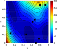
(a) BiPhIK $\mathbf{F}_{r}$

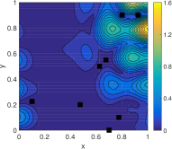
(b) BiPhIK $\hat{s}$

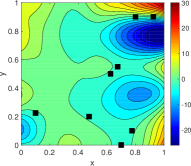
(c) BiPhIK $\mathbf{F}_{r}-\mathbf{F}$

Figure 2: Reconstruction of the modified Branin function by BiPhIK with eight original observations (squares).

There are slight difference betwen the results from CoPhIK and CoBiPhIK as shown in Fig. 3.

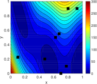
(a) CoPhIK $\mathbf{F}_{r}$

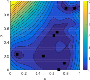
(b) CoPhIK $\hat{s}$

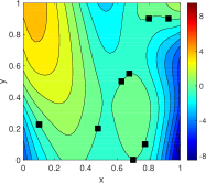
(c) CoPhIK $\mathbf{F}_{r}-\mathbf{F}$

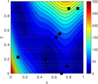
(d) CoBiPhIK $\mathbf{F}_{r}$

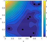
(e) CoBiPhIK $\hat{s}$

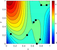
(f) CoBiPhIK $\mathbf{F}_{r}-\mathbf{F}$

Figure 3: Reconstruction of the modified Branin function by CoPhIK and Co-BiPhIK with eight original observations (squares).

We then use a greedy algorithm (in the appendix) that acquires additional observations of the exact field one by one. Fig. 4 presents the comparison of PhIK and BiPhIK when eight additional observations (marked as black stars) are added, which shows a slight difference in the location of additional observations and small discrepancies between the results. Also, Fig. 5 illustrates the difference between CoPhIK and CoBiPhIK, and we see more significant differences in the pattern of $\hat{s}$ and $\bm{F}_{r}-\bm{F}$ than the comparison between PhIK and BiPhIK.

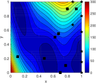
(a) PhIK $\mathbf{F}_{r}$

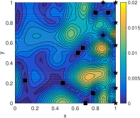
(b) PhIK $\hat{s}$

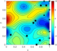
(c) PhIK $\mathbf{F}_{r}-\mathbf{F}$

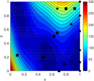
(d) BiPhIK $\mathbf{F}_{r}$

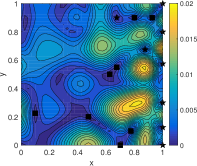
(e) BiPhIK $\hat{s}$

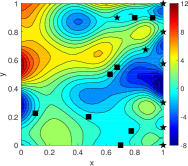
(f) BiPhIK $\mathbf{F}_{r}-\mathbf{F}$

Figure 4: Reconstruction of the modified Branin function by PhIK and BiPhIK with eight original observations (squares) and eight additional observations (stars).

(a) CoPhIK $\mathbf{F}_{r}$

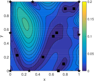
(b) CoPhIK $\hat{s}$

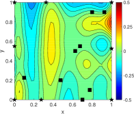
(c) CoPhIK $\mathbf{F}_{r}-\mathbf{F}$

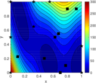
(d) CoBiPhIK $\mathbf{F}_{r}$

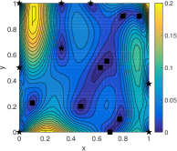
(e) CoBiPhIK $\hat{s}$

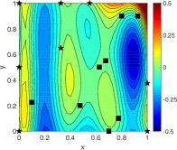
(f) CoBiPhIK $\mathbf{F}_{r}-\mathbf{F}$

Figure 5: Reconstruction of the modified Branin function by CoPhIK and CoBiPhIK with eight original observations (squares) and eight additional observations (stars).

Fig. 6 presents a quantitative study of the difference between the posterior mean and the reference solution with respect to the total number of observation data. The results are consistent with Fig.s 2-5 in that the difference between PhIK and BiPhIK is very small while the difference between CoPhIK and CoBiPhIK is larger. We note that the latter is still very small ranging from $\mathcal{O}(10^{-3})$ to $\mathcal{O}(10^{-2})$ depending on the number of observations. This is because $u_{B}(\Gamma)$ approximates $u_{H}(\Gamma)$ very well in this case. Specifically, $\delta_{1}=0.0279$ and $\delta_{2}=0.0012$.

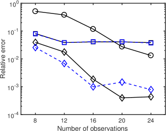
Figure 6: Relative error of reconstructed modified Branin function $\|\bm{F}_{r}-\bm{F}\|_{F}/\|\bm{F}\|_{F}$ using Kriging (“$\,\circ$”), PhIK (blue “$\,\square$”), BiPhIK (black “$\,\square$”), CoPhIK (blue “$\,\diamond$”) and CoBiPhIK (black “$\,\diamond$”) with different numbers of total observations via active learning.

3.2 Heat transfer

In the second example, we consider the steady state of a heat transfer problem. The nondimesionalized heat equation is given as

$$\dfrac{\partial T}{\partial t}-\nabla\cdot(\kappa(T)\nabla T)=0,\quad\bm{x}\in D,$$ (3.3)

where $T(\bm{x},t)$ is the temperature, and the heat conductivity $\kappa$ is set as a function of $T$. The computational domain $D$ is a rectangule $[-0.5,0.5]\times[-0.2,0.2]$ with two circular cavities $R_{1}(O_{1},r_{1})$ and $R_{2}(O_{2},r_{2})$, where $O_{1}=(-0.3,0),O_{2}=(0.2,0),r_{1}=0.1,r_{2}=0.15$ (see Fig. 7). The boundary conditions are given as follows:

$$\begin{dcases}T=-30\cos(2\pi x)+40,&x\in\Gamma_{1};\\ \dfrac{\partial T}{\partial\bm{n}}=-20,&x\in\Gamma_{2};\\ T=30\cos(2\pi(x+0.1))+40,&x\in\Gamma_{3};\\ \dfrac{\partial T}{\partial\bm{n}}=20,&x\in\Gamma_{4};\\ \dfrac{\partial T}{\partial\bm{n}}=0,&x\in\Gamma_{5}.\end{dcases}$$ (3.4)

The “real” conductivity is set as

$$\kappa(T)=1.0+\exp(0.02T),$$ (3.5)

and the profile of the steady state temperature is presented in Fig. 7. This solution is obtained by the finite element method with unstructured triangular mesh using MATLAB PDE toolbox, and the degree of freedom (DOF) is $1319$ (maximum grid size is $0.02$). The observations of this exact profile (denoted as $\mathbf{F}$) are collected at six locations $\{(-0.4,\pm 0.1),(-0.05,\pm 0.1),(0.4,\pm 0.1)\}$ (black squares in Fig. 7).

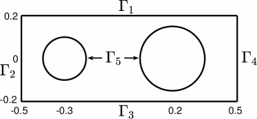
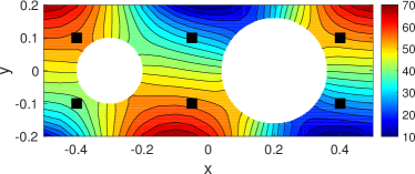
Figure 7: Heat transfer problem. Left: computational domain; right: contours of steady state solution and locations of six observations (black squares).

Now we assume that due to the lack of knowledge, the conductivity is modeled as

$$\kappa(T;\omega)=0.1+\xi T,$$ (3.6)

where $\xi(\omega)$ is a uniform random variable $\mathcal{U}[0.0012,0.0108]$. Apparently, this physical model significantly underestimates the heat conductivity, and its form is incorrect. We generate $M=400$ samples of $\xi(\omega)$ and solve Eq. (3.3) on a coarser grid (maximum grid size is $0.1$) with $\text{DOF}=96$ to obtain corresponding temperature solutions which forms $u_{L}(\Gamma)$. We set $M_{H}=19$ in this example.

It is shown in [46], the Kriging reconstruction is not accurate because of the selection of observations and the property of the exact solution. Fig. 8 presents the results by BiPhIK and CoBiPhIK, and they are very similar to the results by PhIK and CoPhIK in [46] (not shown here), respectively. These results are better than Kriging (see Fig. 11 for quantitative comparison).

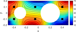
(a) BiPhIK $\mathbf{F}_{r}$

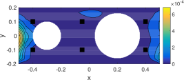
(b) BiPhIK $\hat{s}$

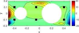
(c) BiPhIK $\mathbf{F}_{r}-\mathbf{F}$

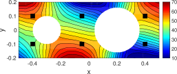
(d) CoBiPhIK $\mathbf{F}_{r}$

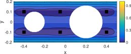
(e) CoBiPhIK $\hat{s}$

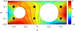
(f) CoBiPhIK $\mathbf{F}_{r}-\mathbf{F}$

Figure 8: Reconstruction of the steady state solution of heat transfer problem by BiPhIK (first row) and CoBiPhIK (second row) with eight original observations (squares).

Next, we adaptively add more observation data one by one. The results by PhIK and BiPhIK are very similar. We only present $\mathbf{F}_{r}$ by these two methods in Fig. 9 for comparison. We can see that the discrepancy in $\mathbf{F}_{r}$ is very insignificant, and there is only a slight difference in the locations of new observations (marked as starts) on the boundary $\Gamma_{2}$. Fig. 10 compares the results by CoPhIK and CoBiPhIK. Although $\mathbf{F}_{r}$ and $\mathbf{F}_{r}-\mathbf{F}$ are similar, there is significant discrepancy in $\hat{s}$, mainly because the correlation length $l_{i}$ in the $Y_{{}_{d}}$’s kernel function are different.

(a) PhIK $\mathbf{F}_{r}$

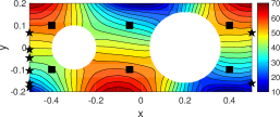
(b) BiPhIK $\mathbf{F}_{r}$

Figure 9: Reconstruction of the steady state solution of heat transfer problem by PhIK and BiPhIK with eight original observations (squares) and eight additional observations (stars).

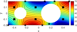
(a) CoPhIK $\mathbf{F}_{r}$

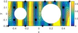
(b) CoPhIK $\hat{s}$

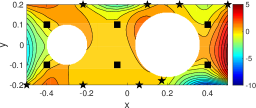
(c) CoPhIK $\mathbf{F}_{r}-\mathbf{F}$

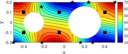
(d) CoBiPhIK $\mathbf{F}_{r}$

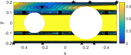
(e) CoBiPhIK $\hat{s}$

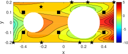
(f) CoBiPhIK $\mathbf{F}_{r}-\mathbf{F}$

Figure 10: Reconstruction of the steady state solution of heat transfer problem by CoPhIK and CoBiPhIK with eight original observations (squares) and eight additional observations (stars).

Fig. 11 presents the quantitative comparison of the relative error by different methods. In this case, the PhIK and BiPhIK results are almost the same, and the CoPhIK and CoBiPhIK results are also very similar. Kriging performs poorly when the number of observations is smaller than $22$, however it outperforms PhIK (and BiPhIK) when $22$ observations are available. CoPhIK (and CoBiPhIK) is always better than Kriging and PhIK (and BiPhIK) as shown in [46]. Again, in this case, $u_{B}(\Gamma)$ approximates $u_{H}(\Gamma)$ very well ($\delta_{1}=0.0039$ and $\delta_{2}=0.0015$), which yields a much smaller difference between PhIK and BiPhIK, and between CoPhIK and CoBiPhIK.

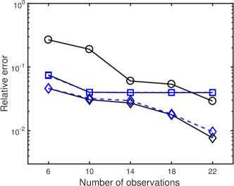
Figure 11: Relative error of reconstructed steady state solution of heat transfer problem $\|\bm{F}_{r}-\bm{F}\|_{F}/\|\bm{F}\|_{F}$ using Kriging (“$\,\circ$”), PhIK (blue “$\,\square$”), BiPhIK (black “$\,\square$”), CoPhIK (blue “$\,\diamond$”) and CoBiPhIK (black “$\,\diamond$”) with different numbers of total observations via active learning.

3.3 Kuramoto-Sivashinsky equation

As a final example, we consider the one-dimensional Kuramoto-Sivashinsy (KS) equation [21, 38]:

$$\begin{split}&u_{t}+4u_{xxxx}+\alpha\left[u_{xx}+\dfrac{1}{2}(u_{x})^{2}\right]=0,\quad 0\leq x\leq 2\pi,\\ &u(x+2\pi,t)=u(x,t),\\ &u(x,0)=u_{0}(x),\end{split}$$ (3.7)

where

$$u_{0}(x)=2.9420\cos(2x)+0.4642\cos(4x)+0.0410\cos(6x)+0.0034\cos(8x).$$ (3.8)

It is well known that this equation can be used to depict a chaotic system, and it is very sensitive to the parameter $\alpha$ when it is large. More importantly, in numerical simulation, high precision is necessary because of the extreme sensitivity of the simulations with respect to numerical accuracy [12, 13]. We use the spectral method for spacial derivatives as in [24]. Specifically, we use Fourier expansion with $256$ terms to obtain the reference solution and $u_{H}$, and use expansion with $128$ terms to compute $u_{L}$. For the time integration, we use a fourth-order Runge-Kutta method [11] with time step $10^{-3}$. We investigate the solution of a KS equation at $T=5$, and the “exact” $\alpha=37.545$. Accurate observations are available at

$$x=\dfrac{12\pi}{256}+\dfrac{56\pi}{256}\cdot j,\quad j=0,1,\dotsc,8.$$

We assume that we do not know the exact $\alpha$, and use the biased “domain knowledge” to set $\alpha$ as a uniform random variable $\mathcal{U}[30,36]$. Apparently, this range is below the exact $\alpha$. We generate $400$ samples of $\alpha$, and compute corresponding $u_{H}^{m}$ and $u_{L}^{m}$ to compare the performance of different methods. Specifically, the we set $M_{H}=17$ to construct $u_{B}(\Gamma)$.

Fig. 12 illustrates the reference solution and the locations of accurate observations. The mean of the $\{u_{H}^{m}\}_{m=1}^{400}$ is illustrated as the dashed line, which deviates from the exact solution significantly with the relative $L_{2}$ error more than $140\%$. We also compute the standard deviation of $u_{H}$ at each $\bm{x}$. Since we will use statistics of $u_{H}$ to construct a GP in PhIK, we present the “$95\%$ confidence interval”, i.e., mean plus minus two standard deviations in Fig. 12. We note that this is not the exact confidence interval of the ensemble $\{u_{H}^{m}\}_{m=1}^{400}$ itself. Fig. 12 shows clearly that the exact solution is not bounded by the confidence interval. This is because in the stochastic model, the $\alpha$ is below its exact value, and the KS equation is very sensitive to $\alpha$.

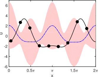
Figure 12: Exact solution of the KS equation (solid line), observations (circles), mean of the realizations (dashed line) and the “$\,95\%$ confidence interval” (shaded area).

Fig. 13 illustrates the Kriging results by using the nine accurate observations. The reconstruction is less accurate near the right end than the other regions, and the uncertainty is larger (i.e., the confidence interval is wider). This is because there is no observation near the right end compared with other regions. Also, the periodic boundary condition is not preserved. Fig. 14 shows the results by PhIK (using $\{u_{H}^{m}\}_{m=1}^{400}$) and BiPhIK (using $\{u_{B}^{m}\}_{m=1}^{400}$). The PhIK performs better than BiPhIK, and, more importantly, the periodic boundary condition is preserved by PhIK, and slightly violated by BiPhIK. We note that in this figure, the confidence intervals in both methods are very narrow ($\sim\mathcal{O}(10^{-2})$). Similar to the examples in [49, 46] and the other two examples in this session, PhIK usually yields a less uncertain result, but this result may not be very accurate because the uncertainty estimate of PhIK relies on its prior covariance, which is totally dependent on the stochasticity of the physical model. Fig. 15 demonstrates the results by CoPhIK and CoBiPhIK. The CoPhIK is the most accurate of all the methods (smallest discrepancy between posterior mean and the exact accuracy) with confidence intervals that cover the reference solution, and the periodic boundary condition is slightly violated. The CoBiPhIK is the least accurate among all the methods.

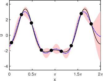
Figure 13: Kriging reconstruction of the KS equation: posterior mean (dashed line), exact solution (solid line), observations (circles), and $95\%$ confidence interval (shaded area).

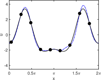
(a) PhIK

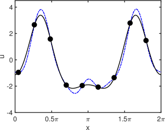
(b) BiPhIK

Figure 14: PhIK (left) and BiPhIK (right) reconstruction of the KS equation: posterior mean (dashed line), exact solution (solid line), observations (circles), and $95\%$ confidence interval (very narrow in this case).

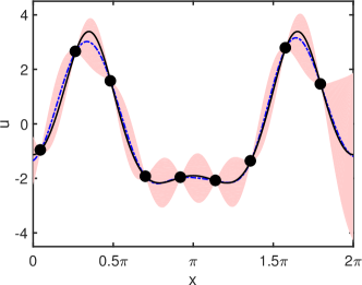
(a) CoPhIK

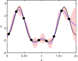
(b) CoBiPhIK

Figure 15: CoPhIK (left) and BiCoPhIK (right) reconstruction of the KS equation: posterior mean (dashed line), exact solution (solid line), observations (circles), and $95\%$ confidence interval (shaded area).

Table 1 presents the relative $L_{2}$ errors of all methods. Different from the previous two examples, in this example, the structures of space $U_{L}(\Gamma)$ and $U_{H}(\Gamma)$ are different because of the sensitivity of the system to the numerical solution, so $u_{B}(\Gamma)$ can not approximate $u_{H}(\Gamma)$ well. Specifically, in this case $\delta_{1}=89.8$ and $\delta_{2}=7.7$. Consequently, the error of BiPhIK is larger than PhIK compared with the other two examples, and the error of CoBiPhIK is much larger than CoPhIK.

Table 1: Relative $L_{2}$ error (posterior mean vs. reference solution) of different methods for reconstructing KS equation solution.

Kriging	PhIK	CoPhIK	BiPhIK	CoBiPhIK
0.1581	0.1145	0.0822	0.1439	0.2477

4 Conclusion

In this work, we extend the PhIK/CoPhIK approach by combining two types of multifidelity methods in the BiPhIK/CoBiPhIK framework to reduce the computational cost of physical models simulations. Specifically, the approximation-theory-based bifidelity method is used to generate approximated high-fidelity realizations of the physical model, which are used to construct GP in PhIK and CoPhIK. The CoKriging approach utilizes an auxiliary GP to describe the discrepancy between the model outputs and the sparse accurate observation data. We present the error estimate of the difference between the posterior mean and variance in the resulting GPs by using BiPhIK/CoBiPhIK and PhIK/CoPhIK. We also analyze the accuracy of preserving linear physical constraints in the posterior mean of BiPhIK/CoBiPhIK.

The presented methods are nonintrusive, and can utilize existing domain codes to compute the necessary realizations. Therefore, these methods are suitable for large-scale complex applications for which physical models and codes are available. When the parametric dependence of the low-fidelity model can well inform the structure of the high-fidelity model, the computational cost can be reduced dramatically.

Our future work would include two directions. One is to use advanced sampling strategies. For example, instead of MC, the probabilistic collocation method is used for the bifidelity method in [27, 51], which can further reduce the computational cost. The other direction is to directly approximate high-fidelity mean and covariance without generating approximated high-fidelity realizations as in [50]. This approach will save the cost of the lifting procedure because it only requires solving a much simpler linear system.

Appendix A Adaptive sampling

In this work, we use a greedy algorithm to add additional observations, i.e., to add new observations at the maxima of $s(\bm{x})$, e.g., [7, 35]. Then, we can make a new prediction $\hat{y}(\bm{x})$ for $\bm{x}\in D$ and compute a new $\hat{s}^{2}(\bm{x})$ to select the next location for additional observation (see Algorithm 3). This selection criterion is based on the statistical interpretation of the interpolation. More sophisticated sensor placement algorithms can be found in literature, e.g., [16, 20, 9], and PhIK/BiPhIK or CoPhIK/CoBiPhIK are complementary to these methods.

Algorithm 3 Active learning based on GPR

1:Specify the locations $\bm{X}$, corresponding observations $\bm{y}$, and the maximum number of observations $N_{\max}$ affordable. The number of available observations is denoted as $N$.

2:while $N_{\max}>N$ do

3:     Compute the MSE $\hat{s}^{2}(\bm{x})$ of prediction $\hat{y}(\bm{x})$ for $\bm{x}\in D$.

4:     Locate the location $\bm{x}_{m}$ for the maximum of $\hat{s}^{2}(\bm{x})$ for $\bm{x}\in D$.

5:     Obtain observation $y_{m}$ at $\bm{x}_{m}$, and set $\bm{X}=\{\bm{X},\bm{x}_{m}\},\bm{y}=(\bm{y}^{\top},y_{m})^{\top},N=N+1$.

6:end while

7:Construct the prediction of $\hat{y}(\bm{x})$ on $D$ using $\bm{X}$ and $\bm{y}$.

Appendix B Proofs of Theorems 2.1 and 2.2

We present the following three lemmas.

Lemma B.1.

For $1\leq n\leq N$,

$$\|k_{H}(\bm{x},\bm{x}^{(n)})\|\leq\sigma_{H}(\Gamma)\sigma_{H}(\bm{x}^{(n)}),$$ (B.1)

$$\|k_{B}(\bm{x},\bm{x}^{(n)})\|\leq\sigma_{B}(\Gamma)\sigma_{B}(\bm{x}^{(n)}).$$

Proof.

According to Eq. (2.19), we have

$$\|k_{H}(\bm{x},\bm{x}^{(n)})\|= \left\|\dfrac{1}{M-1}\sum_{m=1}^{M}\left(u^{m}_{H}(\bm{x})-\mu_{H}(\bm{x})\right)\left(u^{m}_{H}(\bm{x}^{(n)})-\mu_{H}(\bm{x}^{(n)})\right)\right\|$$

$$\leq \dfrac{1}{M-1}\sum_{m=1}^{M}\left\|u^{m}_{H}(\bm{x})-\mu_{H}(\bm{x})\right\|\left|u^{m}_{H}(\bm{x}^{(n)})-\mu_{H}(\bm{x}^{(n)})\right|$$

$$\leq \dfrac{1}{M-1}\left(\sum_{m=1}^{M}\left\|u^{m}_{H}(\bm{x})-\mu_{H}(\bm{x})\right\|^{2}\right)^{\frac{1}{2}}\left(\sum_{m=1}^{M}\left|u^{m}_{H}(\bm{x}^{(n)})-\mu_{H}(\bm{x}^{(n)})\right|^{2}\right)^{\frac{1}{2}}$$

$$= \left(\dfrac{1}{M-1}\sum_{m=1}^{M}\left\|u^{m}_{H}(\bm{x})-\mu_{H}(\bm{x})\right\|^{2}\right)^{\frac{1}{2}}\left(\dfrac{1}{M-1}\sum_{m=1}^{M}\left|u^{m}_{H}(\bm{x}^{(n)})-\mu_{H}(\bm{x}^{(n)})\right|^{2}\right)^{\frac{1}{2}}$$

$$= \sigma_{H}(\Gamma)\sigma_{H}(\bm{x}^{(n)}).$$

Similarly, $\|k_{B}(\bm{x},\bm{x}^{(n)})\|\leq\sigma_{B}(\Gamma)\sigma_{B}(\bm{x}^{(n)})$. ∎

Lemma B.2.

For $1\leq n\leq N$,

$$\left\|k_{H}(\bm{x},\bm{x}^{(n)})-k_{B}(\bm{x},\bm{x}^{(n)})\right\|\leq\dfrac{2}{M-1}\sum_{m=1}^{M}\left(\delta_{1}\left|u^{m}_{B}(\bm{x}^{(n)})-\mu_{B}^{m}(\bm{x}^{(n)})\right|+\delta_{2}\left\|u_{H}^{m}(\bm{x})-\mu_{H}(\bm{x})\right\|\right).$$ (B.2)

Proof.

For any $x\in D$,

$$\left\|\mu_{H}(\bm{x})-\mu_{B}(\bm{x})\right\|=\left\|\dfrac{1}{M}\sum_{m=1}^{M}u_{H}^{m}(\bm{x})-\dfrac{1}{M}\sum_{m=1}^{M}u_{B}^{m}(\bm{x})\right\|\leq\dfrac{1}{M}\sum_{m=1}^{M}\left\|u_{H}^{m}(\bm{x})-u_{B}^{m}(\bm{x})\right\|\leq\delta_{1},$$ (B.3)

and

$$\left|\mu_{H}(\bm{x})-\mu_{B}(\bm{x})\right|=\left|\dfrac{1}{M}\sum_{m=1}^{M}u_{H}^{m}(\bm{x})-\dfrac{1}{M}\sum_{m=1}^{M}u_{B}^{m}(\bm{x})\right|\leq\dfrac{1}{M}\sum_{m=1}^{M}\left|u_{H}^{m}(\bm{x})-u_{B}^{m}(\bm{x})\right|\leq\delta_{2}.$$ (B.4)

Therefore,

$$\left\|k_{H}(\bm{x},\bm{x}^{(n)})-k_{B}(\bm{x},\bm{x}^{(n)})\right\|$$

$$= \dfrac{1}{M-1}\bigg{\|}\sum_{m=1}^{M}\left(u^{m}_{H}(\bm{x})-\mu_{H}(\bm{x})\right)\left(u^{m}_{H}(\bm{x}^{(n)})-\mu_{H}(\bm{x}^{(n)})\right)-\sum_{m=1}^{M}\left(u^{m}_{B}(\bm{x})-\mu_{B}(\bm{x})\right)\left(u^{m}_{B}(\bm{x}^{(n)})-\mu_{B}(\bm{x}^{(n)})\right)\bigg{\|}$$

$$\leq \dfrac{1}{M-1}\sum_{m=1}^{M}\bigg{\{}\bigg{\|}\left(u^{m}_{H}(\bm{x})-\mu_{H}(\bm{x})\right)\left(u^{m}_{H}(\bm{x}^{(n)})-\mu_{H}(\bm{x}^{(n)})\right)-\left(u^{m}_{H}(\bm{x})-\mu_{H}(\bm{x})\right)\left(u^{m}_{B}(\bm{x}^{(n)})-\mu_{B}(\bm{x}^{(n)})\right)\bigg{\|}$$

$$\qquad\qquad~{}~{}+\bigg{\|}\left(u^{m}_{H}(\bm{x})-\mu_{H}(\bm{x})\right)\left(u^{m}_{B}(\bm{x}^{(n)})-\mu_{B}(\bm{x}^{(n)})\right)-\left(u^{m}_{B}(\bm{x})-\mu_{B}(\bm{x})\right)\left(u^{m}_{B}(\bm{x}^{(n)})-\mu_{B}(\bm{x}^{(n)})\right)\bigg{\|}\bigg{\}}$$

$$\leq \dfrac{1}{M-1}\sum_{m=1}^{M}\bigg{\{}\left\|u^{m}_{H}(\bm{x})-\mu_{H}(\bm{x})\right\|\left|u^{m}_{H}(\bm{x}^{(n)})-\mu_{H}(\bm{x}^{(n)})-u^{m}_{B}(\bm{x}^{(n)})+\mu_{B}(\bm{x}^{(n)})\right|$$

$$\qquad\qquad\quad+\left|u^{m}_{B}(\bm{x}^{(n)})-\mu_{B}(\bm{x}^{(n)})\right|\left\|u^{m}_{H}(\bm{x})-\mu_{H}(\bm{x})-u^{m}_{B}(\bm{x})+\mu_{B}(\bm{x})\right\|\bigg{\}}$$

$$\leq \dfrac{1}{M-1}\sum_{m=1}^{M}\bigg{\{}2\delta_{2}\left\|u^{m}_{H}(\bm{x})-\mu_{H}(\bm{x})\right\|+2\delta_{1}\left|u^{m}_{B}(\bm{x}^{(n)})-\mu_{B}(\bm{x}^{(n)})\right|\bigg{\}}.$$

∎

Lemma B.3.

For $1\leq i,j\leq N$,

$$\left|k_{H}(\bm{x}^{(i)},\bm{x}^{(j)})-k_{B}(\bm{x}^{(i)},\bm{x}^{(j)})\right|\leq 2\delta_{2}\sqrt{\dfrac{M}{M-1}}\left[\sigma_{H}(\bm{x}^{(i)})+\sigma_{B}(\bm{x}^{(j)})\right].$$ (B.5)

Proof.

$$\left|k_{H}(\bm{x}^{(i)},\bm{x}^{(j)})-k_{B}(\bm{x}^{(i)},\bm{x}^{(j)})\right|$$

$$= \dfrac{1}{M-1}\bigg{|}\sum_{m=1}^{M}\left(u^{m}_{H}(\bm{x}^{(i)})-\mu_{H}(\bm{x}^{(i)})\right)\left(u^{m}_{H}(\bm{x}^{(j)})-\mu_{H}(\bm{x}^{(j)})\right)$$

$$\qquad\quad-\sum_{m=1}^{M}\left(u^{m}_{B}(\bm{x}^{(i)})-\mu_{B}(\bm{x}^{(i)})\right)\left(u^{m}_{B}(\bm{x}^{(j)})-\mu_{B}(\bm{x}^{(j)})\right)\bigg{|}$$

$$\leq \dfrac{1}{M-1}\sum_{m=1}^{M}\bigg{\{}\bigg{|}\left(u^{m}_{H}(\bm{x}^{(i)})-\mu_{H}(\bm{x}^{(i)})\right)\left(u^{m}_{H}(\bm{x}^{(j)})-\mu_{H}(\bm{x}^{(j)})\right)$$

$$\qquad\qquad\qquad-\left(u^{m}_{H}(\bm{x}^{(i)})-\mu_{H}(\bm{x}^{(i)})\right)\left(u^{m}_{B}(\bm{x}^{(j)})-\mu_{B}(\bm{x}^{(j)})\right)\bigg{|}$$

$$\qquad\qquad~{}~{}+\bigg{|}\left(u^{m}_{H}(\bm{x}^{(i)})-\mu_{H}(\bm{x}^{(i)})\right)\left(u^{m}_{B}(\bm{x}^{(j)})-\mu_{B}(\bm{x}^{(j)})\right)$$

$$\qquad\qquad\qquad-\left(u^{m}_{B}(\bm{x}^{(i)})-\mu_{B}(\bm{x}^{(i)})\right)\left(u^{m}_{B}(\bm{x}^{(j)})-\mu_{B}(\bm{x}^{(j)})\right)\bigg{|}\bigg{\}}$$

$$\leq \dfrac{1}{M-1}\sum_{m=1}^{M}\bigg{\{}\left|u^{m}_{H}(\bm{x}^{(i)})-\mu_{H}(\bm{x}^{(i)})\right|\left|u^{m}_{H}(\bm{x}^{(j)})-\mu_{H}(\bm{x}^{(j)})-u^{m}_{B}(\bm{x}^{(j)})+\mu_{B}(\bm{x}^{(j)})\right|$$

$$\qquad\qquad~{}~{}+\left|u^{m}_{B}(\bm{x}^{(j)})-\mu_{B}(\bm{x}^{(j)})\right|\left|u^{m}_{H}(\bm{x}^{(i)})-\mu_{H}(\bm{x}^{(i)})-u^{m}_{B}(\bm{x}^{(i)})+\mu_{B}(\bm{x}^{(i)})\right|\bigg{\}}$$

$$\leq \dfrac{2\delta_{2}}{M-1}\sum_{m=1}^{M}\bigg{\{}\left|u^{m}_{H}(\bm{x}^{(i)})-\mu_{H}(\bm{x}^{(i)})\right|+\left|u^{m}_{B}(\bm{x}^{(j)})-\mu_{B}(\bm{x}^{(j)})\right|\bigg{\}}$$

$$\leq \dfrac{2\delta_{2}\sqrt{M}}{M-1}\left\{\left(\sum_{m=1}^{M}\left|u^{m}_{H}(\bm{x}^{(i)})-\mu_{H}(\bm{x}^{(i)})\right|^{2}\right)^{\frac{1}{2}}+\left(\sum_{m=1}^{M}\left|u^{m}_{B}(\bm{x}^{(j)})-\mu_{B}(\bm{x}^{(j)})\right|^{2}\right)^{\frac{1}{2}}\right\}$$

$$= 2\delta_{2}\sqrt{\dfrac{M}{M-1}}\left[\sigma_{H}(\bm{x}^{(i)})+\sigma_{B}(\bm{x}^{(j)})\right].$$

∎

Now we prove Theorem 2.1 as follows.

Proof.

Rewriting Eq. (2.21) in the functional form, we have

$$\hat{y}_{H}(\bm{x})=\mu_{H}(\bm{x})+\sum_{n=1}^{N}a_{n}^{H}k_{H}(\bm{x},\bm{x}^{(n)}),$$ (B.6)

where $a_{n}^{H}$ is the $n$-th entry of the vector $\mathbf{C}_{H}^{-1}(\bm{y}-\bm{\mu}_{H})$, $(\mathbf{C}_{H})_{ij}=k_{H}(\bm{x}^{(i)},\bm{x}^{(j)})$ and $(\bm{\mu}_{H})_{i}=\mu_{H}(\bm{x}^{(i)})$. Similarly, we have

$$\hat{y}_{B}(\bm{x})=\mu_{B}(\bm{x})+\sum_{n=1}^{N}a_{n}^{B}k_{B}(\bm{x},\bm{x}^{(n)}),$$ (B.7)

where $a_{n}^{B}$ is the $n$-th entry of the vector $\mathbf{C}_{B}^{-1}(\bm{y}-\bm{\mu}_{B})$, $(\mathbf{C}_{B})_{ij}=k_{B}(\bm{x}^{(i)},\bm{x}^{(j)})$ and $(\bm{\mu}_{B})_{i}=\mu_{B}(\bm{x}^{(i)})$. In Eq. (B.3), we show that

$$\left\|\mu_{H}(\bm{x})-\mu_{B}(\bm{x})\right\|\leq\delta_{1}.$$

Next,

$$\left\|a^{H}_{n}k_{H}(\bm{x},\bm{x}^{(n)})-a^{B}_{n}k_{B}(\bm{x},\bm{x}^{(n)})\right\|$$

$$\leq \left\|a^{H}_{n}k_{H}(\bm{x},\bm{x}^{(n)})-a^{B}_{n}k_{H}(\bm{x},\bm{x}^{(n)})\right\|+\left\|a^{B}_{n}k_{H}(\bm{x},\bm{x}^{(n)})-a^{B}_{n}k_{B}(\bm{x},\bm{x}^{(n)})\right\|$$

$$\leq \left|a^{H}_{n}-a^{B}_{n}\right|\left\|k_{H}(\bm{x},\bm{x}^{(n)})\right\|+\left|a^{B}_{n}\right|\left\|k_{H}(\bm{x},\bm{x}^{(n)})-k_{B}(\bm{x},\bm{x}^{(n)})\right\|$$

$$\leq \left|a^{H}_{n}-a^{B}_{n}\right|\sigma_{H}(\Gamma)\sigma_{H}(\bm{x}^{(n)})+\dfrac{2\left|a^{B}_{n}\right|}{M-1}\sum_{m=1}^{M}\left(\delta_{1}\left|u^{m}_{B}(\bm{x}^{(n)})-\mu_{B}^{m}(\bm{x}^{(n)})\right|+\delta_{2}\left\|u_{H}^{m}(\bm{x})-\mu_{H}(\bm{x})\right\|\right),$$

where the last inequality utilizes Lemmas B.1 and B.2. Therefore,

$$\left\|\sum_{n=1}^{N}a^{H}_{n}k_{H}(\bm{x},\bm{x}^{(n)})-\sum_{n=1}^{N}a^{B}_{n}k_{B}(\bm{x},\bm{x}^{(n)})\right\|$$

$$\leq \underbrace{\sum_{n=1}^{N}\left|a^{H}_{n}-a^{B}_{n}\right|\sigma_{H}(\Gamma)\sigma_{H}(\bm{x}^{(n)})}_{J_{1}}+\underbrace{\dfrac{2\delta_{1}}{M-1}\sum_{n=1}^{N}\left|a_{n}^{B}\right|\sum_{m=1}^{M}\left|u^{m}_{B}(\bm{x}^{(n)})-\mu_{B}^{m}(\bm{x}^{(n)})\right|}_{J_{2}}$$

$$+\underbrace{\dfrac{2\delta_{2}}{M-1}\sum_{n=1}^{N}\left|a_{n}^{B}\right|\sum_{m=1}^{M}\left\|u^{m}_{H}(\bm{x})-\mu_{H}^{m}(\bm{x})\right\|}_{J_{3}}.$$

Here,

$$J_{1} =\sigma_{H}(\Gamma)\sum_{n=1}^{N}\left|a^{H}_{n}-a^{B}_{n}\right|\sigma_{H}(\bm{x}^{(n)})$$

$$\leq\sigma_{H}(\Gamma)\left(\sum_{n=1}^{N}\sigma^{2}_{H}(\bm{x}^{(n)}))\right)^{\frac{1}{2}}\left(\sum_{n=1}^{N}\left|a^{H}_{n}-a^{B}_{n}\right|^{2}\right)^{\frac{1}{2}}$$

$$=S_{H}\sigma_{H}(\Gamma)\left\|\mathbf{C}_{H}^{-1}(\bm{y}-\bm{\mu}_{H})-\mathbf{C}_{B}^{-1}(\bm{y}-\bm{\mu}_{B})\right\|_{2}$$

$$=S_{H}\sigma_{H}(\Gamma)\left\|\mathbf{C}_{H}^{-1}(\bm{y}-\bm{\mu}_{H})-\mathbf{C}_{H}^{-1}(\bm{y}-\bm{\mu}_{B})+\mathbf{C}_{H}^{-1}(\bm{y}-\bm{\mu}_{B})-\mathbf{C}_{B}^{-1}(\bm{y}-\bm{\mu}_{B})\right\|_{2}$$

$$\leq S_{H}\sigma_{H}(\Gamma)\left(\left\|\mathbf{C}_{H}^{-1}\right\|_{2}\left\|\bm{\mu}_{H}-\bm{\mu}_{B}\right\|_{2}+\left\|\mathbf{C}_{H}^{-1}-\mathbf{C}_{B}^{-1}\right\|_{2}\left\|\bm{y}-\bm{\mu}_{B}\right\|_{2}\right)$$

$$\leq S_{H}\sigma_{H}(\Gamma)\left\{\left\|\mathbf{C}_{H}^{-1}\right\|_{2}\sqrt{N}\delta_{2}+\left\|\mathbf{C}_{H}^{-1}\right\|_{2}^{2}\left\|\mathbf{C}_{H}-\mathbf{C}_{B}\right\|_{2}\left\|\bm{y}-\bm{\mu}_{B}\right\|_{2}\right\}$$

$$\leq S_{H}\sigma_{H}(\Gamma)\left\{\left\|\mathbf{C}_{H}^{-1}\right\|_{2}\sqrt{N}\delta_{2}+\left\|\mathbf{C}_{H}^{-1}\right\|_{2}^{2}\left\|\mathbf{C}_{H}-\mathbf{C}_{B}\right\|_{F}\left\|\bm{y}-\bm{\mu}_{B}\right\|_{2}\right\},$$

where we uses the well-known matrix perturbation conclusion (e.g., [3]):

$$\left\|(\mathbf{A}+\Delta\mathbf{A})^{-1}-\mathbf{A}^{-1}\right\|\leq\left\|\mathbf{A}^{-1}\right\|^{2}\|\Delta\mathbf{A}\|$$ (B.8)

for invertible matrices $\mathbf{A}$ and $\mathbf{A}+\Delta\mathbf{A}$, and a well-defined matrix norm $\|\cdot\|$. Further, using Lemma B.3, we have

$$\left\|\mathbf{C}_{H}-\mathbf{C}_{B}\right\|^{2}_{F}= \sum_{i=1}^{N}\sum_{j=1}^{N}\left|k_{H}(\bm{x}^{(i)},\bm{x}^{(j)})-k_{B}(\bm{x}^{(i)},\bm{x}^{(j)})\right|^{2}$$ (B.9)

$$\leq \sum_{i=1}^{N}\sum_{j=1}^{N}\dfrac{4\delta_{2}^{2}M}{M-1}\left[\sigma(u_{H}^{m}(\bm{x}^{(i)}))+\sigma(u_{B}^{m}(\bm{x}^{(j)}))\right]^{2}$$

$$\leq \dfrac{8\delta_{2}^{2}M}{M-1}\sum_{i=1}^{N}\sum_{j=1}^{N}\left[\sigma^{2}(u_{H}^{m}(\bm{x}^{(i)}))+\sigma^{2}(u_{B}^{m}(\bm{x}^{(j)}))\right]$$

$$= \dfrac{8\delta_{2}^{2}MN}{M-1}\sum_{n=1}^{N}\left[\sigma^{2}(u_{H}^{m}(\bm{x}^{(n)}))+\sigma^{2}(u_{B}^{m}(\bm{x}^{(n)}))\right]$$

$$= \dfrac{8\delta_{2}^{2}MN}{M-1}(S^{2}_{H}+S^{2}_{B})$$

which yields

$$J_{1}\leq\sqrt{N}S_{H}\delta_{2}\sigma_{H}(\Gamma)\left\|\mathbf{C}_{H}^{-1}\right\|_{2}\left\{2\sqrt{\dfrac{2M}{M-1}}\left(S^{2}_{H}+S^{2}_{B}\right)^{\frac{1}{2}}\left\|\mathbf{C}_{H}^{-1}\right\|_{2}\|\bm{y}-\bm{\mu}_{B}\|_{2}+1\right\}.$$

Also,

$$J_{2}\leq 2\delta_{1}\sqrt{\dfrac{M}{M-1}}\sum_{n=1}^{N}\left|a_{n}^{B}\right|\sigma(u_{B}^{m}(\bm{x}^{(n)}))$$

$$\leq 2\delta_{1}\sqrt{\dfrac{MN}{M-1}}\left\|\mathbf{C}_{B}^{-1}(\bm{y}-\bm{\mu}_{B})\right\|_{2}\left(\sum_{n=1}^{N}\sigma^{2}(u_{B}^{m}(\bm{x}^{(n)}))\right)^{\frac{1}{2}}$$

$$\leq 2\delta_{1}\sqrt{\dfrac{MN}{M-1}}\left\|\mathbf{C}_{B}^{-1}\right\|_{2}\left\|\bm{y}-\bm{\mu}_{B}\right\|_{2}S_{B}$$

Similarly,

$$J_{3}\leq 2\delta_{2}\sqrt{\dfrac{M}{M-1}}\sum_{n=1}^{N}\left|a_{n}^{B}\right|\sigma_{H}(\Gamma)$$

$$\leq 2\delta_{2}\sqrt{\dfrac{MN}{M-1}}\sigma_{H}(\Gamma)\left\|\mathbf{C}_{B}^{-1}(\bm{y}-\bm{\mu}_{B})\right\|_{2}$$

$$\leq 2\delta_{2}\sqrt{\dfrac{MN}{M-1}}\sigma_{H}(\Gamma)\left\|\mathbf{C}_{B}^{-1}\right\|_{2}\left\|\bm{y}-\bm{\mu}_{B}\right\|_{2}.$$

Therefore, the conclusion holds. ∎

Next, we present the proof of Theorem 2.2.

Proof.

For any $\bm{x}^{*}\in D$, we use the following concise notations

$$\bm{c}_{H} =\left(k_{H}(\bm{x}^{(1)},\bm{x}^{*}),\dotsc,k_{H}(\bm{x}^{(N)},\bm{x}^{*})\right)^{\top},$$ (B.10)

$$\bm{c}_{B} =\left(k_{B}(\bm{x}^{(1)},\bm{x}^{*}),\dotsc,k_{B}(\bm{x}^{(N)},\bm{x}^{*})\right)^{\top}.$$

Following the same procedure in the proof of Lemma B.3, we have

$$\left|k_{H}(\bm{x}^{*},\bm{x}^{*})-k_{B}(\bm{x}^{*},\bm{x}^{*})\right|\leq 2\delta_{2}\sqrt{\dfrac{M}{M-1}}\left[\sigma(u_{H}^{m}(\bm{x}^{*}))+\sigma(u_{B}^{m}(\bm{x}^{*}))\right]\leq 2\delta_{2}\sqrt{\dfrac{2M}{M-1}}(\Delta_{H}^{2}+\Delta_{B}^{2})^{\frac{1}{2}}.$$

According to Lemma B.3,

$$\|\bm{c}_{H}-\bm{c}_{B}\|_{2}= \left(\sum_{n=1}^{N}\left|k_{H}(\bm{x}^{(n)},\bm{x}^{*})-k_{B}(\bm{x}^{(n)},\bm{x}^{*})\right|^{2}\right)^{\frac{1}{2}}$$

$$\leq 2\delta_{2}\sqrt{\dfrac{M}{M-1}}\left(\sum_{n=1}^{N}\left[\sigma(u_{H}^{m}(\bm{x}^{(n)}))+\sigma(u_{B}^{m}(\bm{x}^{*}))\right]^{2}\right)^{\frac{1}{2}}$$

$$\leq 2\delta_{2}\sqrt{\dfrac{2M}{M-1}}\left(\sum_{n=1}^{N}\left[\sigma^{2}(u_{H}^{m}(\bm{x}^{(n)}))+\sigma^{2}(u_{B}^{m}(\bm{x}^{*}))\right]\right)^{\frac{1}{2}}$$

$$= 2\delta_{2}\sqrt{\dfrac{2M}{M-1}}\left(S_{H}^{2}+S_{B}^{2}\right)^{\frac{1}{2}}.$$

Also,

$$\|\bm{c}_{H}\|_{2}= \left\{\sum_{n=1}^{N}\left|k_{H}(\bm{x}^{(n)},\bm{x}^{*})\right|^{2}\right\}^{\frac{1}{2}}$$ (B.11)

$$\leq \Bigg{\{}\sum_{n=1}^{N}\left|\dfrac{1}{M-1}\sum_{m=1}^{M}\left(u^{m}_{H}(\bm{x}^{(n)})-\mu_{H}(\bm{x}^{(n)})\right)\left(u^{m}_{H}(\bm{x}^{*})-\mu_{H}(\bm{x}^{*})\right)\right|^{2}\Bigg{\}}^{\frac{1}{2}}$$

$$\leq \Bigg{\{}\sum_{n=1}^{N}\left(\dfrac{1}{M-1}\sum_{m=1}^{M}\left(u^{m}_{H}(\bm{x}^{(n)})-\mu_{H}(\bm{x}^{(n)})\right)^{2}\right)\cdot\left(\dfrac{1}{M-1}\sum_{m=1}^{M}\left(u^{m}_{H}(\bm{x}^{*})-\mu_{H}(\bm{x}^{*})\right)^{2}\right)\Bigg{\}}^{\frac{1}{2}}$$

$$= \sigma_{H}(\bm{x}^{*})S_{H}.$$

Similarly,

$$\|\bm{c}_{B}\|_{2}\leq\sigma_{B}(\bm{x}^{*})S_{B}.$$ (B.12)

Thus,

$$\left|\bm{c}_{H}^{\top}\mathbf{C}_{H}^{-1}\bm{c}_{H}-\bm{c}_{B}^{\top}\mathbf{C}_{B}^{-1}\bm{c}_{B}\right|$$ (B.13)

$$\leq \left|\bm{c}_{H}^{\top}\mathbf{C}_{H}^{-1}\bm{c}_{H}-\bm{c}_{H}^{\top}\mathbf{C}_{H}^{-1}\bm{c}_{B}\right|+\left|\bm{c}_{H}^{\top}\mathbf{C}_{H}^{-1}\bm{c}_{B}-\bm{c}_{H}^{\top}\mathbf{C}_{B}^{-1}\bm{c}_{B}\right|+\left|\bm{c}_{H}^{\top}\mathbf{C}_{B}^{-1}\bm{c}_{B}-\bm{c}_{B}^{\top}\mathbf{C}_{B}^{-1}\bm{c}_{B}\right|$$

$$\leq \underbrace{\|\bm{c}_{H}\|_{2}\|\mathbf{C}_{H}^{-1}\|_{2}\|\bm{c}_{H}-\bm{c}_{B}\|_{2}}_{J_{1}}+\underbrace{\|\bm{c}_{H}\|_{2}\|\mathbf{C}_{H}^{-1}-\mathbf{C}_{B}^{-1}\|_{F}\|\bm{c}_{B}\|_{2}}_{J_{2}}+\underbrace{\|\bm{c}_{B}\|_{2}\|\mathbf{C}_{B}^{-1}\|_{2}\|\bm{c}_{H}-\bm{c}_{B}\|_{2}}_{J_{3}},$$

and

$$J_{1} \leq 2\delta_{2}\sqrt{\dfrac{2M}{M-1}}\sigma_{H}(\bm{x}^{*})S_{H}(S_{B}^{2}+S_{H}^{2})^{\frac{1}{2}}\|\mathbf{C}_{H}^{-1}\|_{2},$$

$$J_{2} \leq 2\delta_{2}\sqrt{\dfrac{2MN}{M-1}}\sigma_{H}(\bm{x}^{*})\sigma_{B}(\bm{x}^{*})S_{H}S_{B}(S_{H}^{2}+S_{B}^{2})^{\frac{1}{2}}\|\mathbf{C}_{H}^{-1}\|^{2}_{2},$$

$$J_{3} \leq 2\delta_{2}\sqrt{\dfrac{2M}{M-1}}\sigma_{B}(\bm{x}^{*})S_{B}(S_{B}^{2}+S_{H}^{2})^{\frac{1}{2}}\|\mathbf{C}_{B}^{-1}\|_{2},$$

where in the inequality of $J_{2}$ we use Eqs. (B.8) and (B.9). Finally, using the fact $\sigma_{H}(\bm{x}^{*})\leq\Delta_{H}$ and $\sigma_{B}(\bm{x}^{*})\leq\Delta_{B}$, we have

$$S_{H}\leq\sqrt{N}\Delta_{H},\quad S_{B}\leq\sqrt{N}\Delta_{B},$$ (B.14)

which indicates

$$J_{1} \leq 2N\delta_{2}\sqrt{\dfrac{2M}{M-1}}\Delta^{2}_{H}(\Delta_{B}^{2}+\Delta_{H}^{2})^{\frac{1}{2}}\|\mathbf{C}_{H}^{-1}\|_{2},$$

$$J_{2} \leq 2N\delta_{2}\sqrt{\dfrac{2MN}{M-1}}\Delta^{2}_{H}\Delta^{2}_{B}(\Delta_{H}^{2}+\Delta_{B}^{2})^{\frac{1}{2}}\|\mathbf{C}_{H}^{-1}\|^{2}_{2},$$

$$J_{3} \leq 2N\delta_{2}\sqrt{\dfrac{2M}{M-1}}\Delta^{2}_{B}(\Delta_{B}^{2}+\Delta_{H}^{2})^{\frac{1}{2}}\|\mathbf{C}_{B}^{-1}\|_{2}.$$

Therefore, the conclusion holds. ∎

References

- [1] Christopher James Brooks, AIJ Forrester, AJ Keane, and S Shahpar. Multi-fidelity design optimisation of a transonic compressor rotor. 2011.
- [2] K Andrew Cliffe, Mike B Giles, Robert Scheichl, and Aretha L Teckentrup. Multilevel Monte Carlo methods and applications to elliptic PDEs with random coefficients. Computing and Visualization in Science, 14(1):3, 2011.
- [3] James Demmel. The componentwise distance to the nearest singular matrix. SIAM Journal on Matrix Analysis and Applications, 13(1):10–19, 1992.
- [4] Alireza Doostan and Houman Owhadi. A non-adapted sparse approximation of pdes with stochastic inputs. Journal of Computational Physics, 230(8):3015–3034, 2011.
- [5] Michael S Eldred, Leo WT Ng, Matthew F Barone, and Stefan P Domino. Multifidelity uncertainty quantification using spectral stochastic discrepancy models. Handbook of Uncertainty Quantification, pages 991–1036, 2017.
- [6] Hillary R Fairbanks, Alireza Doostan, Christian Ketelsen, and Gianluca Iaccarino. A low-rank control variate for multilevel monte carlo simulation of high-dimensional uncertain systems. Journal of Computational Physics, 341:121–139, 2017.
- [7] Alexander Forrester, Andy Keane, and Andràs Sòbester. Engineering Design via Surrogate Modelling: A Practical Guide. John Wiley & Sons, 2008.
- [8] Alexander IJ Forrester, András Sóbester, and Andy J Keane. Multi-fidelity optimization via surrogate modelling. In Proceedings of the Royal Society of London A: mathematical, physical and engineering sciences, volume 463, pages 3251–3269. The Royal Society, 2007.
- [9] Roman Garnett, Michael A Osborne, and Stephen J Roberts. Bayesian optimization for sensor set selection. In Proceedings of the 9th ACM/IEEE international conference on Information Processing in Sensor Networks, pages 209–219. ACM, 2010.
- [10] Michael B Giles. Multilevel Monte Carlo path simulation. Operations Research, 56(3):607–617, 2008.
- [11] Sigal Gottlieb, Chi-Wang Shu, and Eitan Tadmor. Strong stability-preserving high-order time discretization methods. SIAM review, 43(1):89–112, 2001.
- [12] James M Hyman and Basil Nicolaenko. The kuramoto-sivashinsky equation: a bridge between pde’s and dynamical systems. Physica D: Nonlinear Phenomena, 18(1-3):113–126, 1986.
- [13] James M Hyman, Basil Nicolaenko, and Stéphane Zaleski. Order and complexity in the kuramoto-sivashinsky model of weakly turbulent interfaces. Physica D: Nonlinear Phenomena, 23(1-3):265–292, 1986.
- [14] Lluis Jofre, Gianluca Geraci, Hillary Fairbanks, Alireza Doostan, and Gianluca Iaccarino. Multi-fidelity uncertainty quantification of irradiated particle-laden turbulence. arXiv preprint arXiv:1801.06062, 2018.
- [15] Brandon A Jones and Ryan Weisman. Multi-fidelity orbit uncertainty propagation. Acta Astronautica, 2018.
- [16] Donald R Jones, Matthias Schonlau, and William J Welch. Efficient global optimization of expensive black-box functions. Journal of Global optimization, 13(4):455–492, 1998.
- [17] Marc C Kennedy and Anthony O’Hagan. Predicting the output from a complex computer code when fast approximations are available. Biometrika, 87(1):1–13, 2000.
- [18] Peter K Kitanidis. Introduction to Geostatistics: Applications in Hydrogeology. Cambridge University Press, 1997.
- [19] M Knotters, DJ Brus, and JH Oude Voshaar. A comparison of kriging, co-kriging and kriging combined with regression for spatial interpolation of horizon depth with censored observations. Geoderma, 67(3-4):227–246, 1995.
- [20] Andreas Krause, Ajit Singh, and Carlos Guestrin. Near-optimal sensor placements in Gaussian processes: Theory, efficient algorithms and empirical studies. Journal of Machine Learning Research, 9(Feb):235–284, 2008.
- [21] Yoshiki Kuramoto. Diffusion-induced chaos in reaction systems. Progress of Theoretical Physics Supplement, 64:346–367, 1978.
- [22] Julien Laurenceau and P Sagaut. Building efficient response surfaces of aerodynamic functions with kriging and cokriging. AIAA journal, 46(2):498–507, 2008.
- [23] Loic Le Gratiet and Josselin Garnier. Recursive co-kriging model for design of computer experiments with multiple levels of fidelity. International Journal for Uncertainty Quantification, 4(5), 2014.
- [24] Jing Li and Panos Stinis. A unified framework for mesh refinement in random and physical space. Journal of Computational Physics, 323:243–264, 2016.
- [25] Xiang Ma and Nicholas Zabaras. An adaptive high-dimensional stochastic model representation technique for the solution of stochastic partial differential equations. Journal of Computational Physics, 229(10):3884–3915, 2010.
- [26] Ramakanth Munipalli, Jason Hamilton, and Xueyu Zhu. A multifidelity approach to parameter dependent modeling of combustion instability. In 2018 Joint Propulsion Conference, page 4557, 2018.
- [27] Akil Narayan, Claude Gittelson, and Dongbin Xiu. A stochastic collocation algorithm with multifidelity models. SIAM Journal on Scientific Computing, 36(2):A495–A521, 2014.
- [28] Leo Wai-Tsun Ng and Michael Eldred. Multifidelity uncertainty quantification using non-intrusive polynomial chaos and stochastic collocation. In 53rd AIAA/ASME/ASCE/AHS/ASC Structures, Structural Dynamics and Materials Conference 20th AIAA/ASME/AHS Adaptive Structures Conference 14th AIAA, page 1852, 2012.
- [29] Harald Niederreiter. Random Number Generation and Quasi-Monte Carlo Methods, volume 63. SIAM, 1992.
- [30] Wenxiao Pan, Xiu Yang, Jie Bao, and Michelle Wang. Optimizing discharge capacity of li-o2 batteries by design of air-electrode porous structure: Multifidelity modeling and optimization. Journal of The Electrochemical Society, 164(11):E3499–E3511, 2017.
- [31] Benjamin Peherstorfer, Tiangang Cui, Youssef Marzouk, and Karen Willcox. Multifidelity importance sampling. Computer Methods in Applied Mechanics and Engineering, 300:490–509, 2016.
- [32] Benjamin Peherstorfer, Karen Willcox, and Max Gunzburger. Optimal model management for multifidelity monte carlo estimation. SIAM Journal on Scientific Computing, 38(5):A3163–A3194, 2016.
- [33] P Perdikaris, D Venturi, JO Royset, and GE Karniadakis. Multi-fidelity modelling via recursive co-kriging and Gaussian–Markov random fields. Proc. R. Soc. A, 471(2179):20150018, 2015.
- [34] Paris Perdikaris, Maziar Raissi, Andreas Damianou, ND Lawrence, and George Em Karniadakis. Nonlinear information fusion algorithms for data-efficient multi-fidelity modelling. Proc. R. Soc. A, 473(2198):20160751, 2017.
- [35] Maziar Raissi, Paris Perdikaris, and George Em Karniadakis. Machine learning of linear differential equations using Gaussian processes. Journal of Computational Physics, 348:683–693, 2017.
- [36] M Razi, A Narayan, RM Kirby, and D Bedrov. Fast predictive models based on multi-fidelity sampling of properties in molecular dynamics simulations. Computational Materials Science, 152:125–133, 2018.
- [37] Jerome Sacks, William J Welch, Toby J Mitchell, and Henry P Wynn. Design and analysis of computer experiments. Statistical Science, pages 409–423, 1989.
- [38] GI Sivashinsky. On flame propagation under conditions of stoichiometry. SIAM Journal on Applied Mathematics, 39(1):67–82, 1980.
- [39] A Stein and LCA Corsten. Universal kriging and cokriging as a regression procedure. Biometrics, pages 575–587, 1991.
- [40] Michael L Stein. Interpolation of Spatial Data: Some Theory for Kriging. Springer Science & Business Media, 2012.
- [41] A. M. Tartakovsky, M. Panzeri, G. D. Tartakovsky, and A. Guadagnini. Uncertainty quantification in scale-dependent models of flow in porous media. Water Resources Research, 53:9392–9401, 2017.
- [42] Menner A Tatang. Direct incorporation of uncertainty in chemical and environmental engineering systems. PhD thesis, Massachusetts Institute of Technology, 1995.
- [43] Rui Tuo, CF Jeff Wu, and Dan Yu. Surrogate modeling of computer experiments with different mesh densities. Technometrics, 56(3):372–380, 2014.
- [44] Christopher KI Williams and Carl Edward Rasmussen. Gaussian processes for machine learning. The MIT Press, 2(3):4, 2006.
- [45] Dongbin Xiu and Jan S. Hesthaven. High-order collocation methods for differential equations with random inputs. SIAM Journal on Scientific Computing, 27(3):1118–1139, 2005.
- [46] Xiu Yang, David Barajas-Solano, Guzel Tartakovsky, Nathan Baker, and Alexandre Tartakovsky. Physics-informed CoKriging: A Gaussian-process-regression-based multifidelity method for data-model convergence. arXiv preprint arXiv:1811.09757, 2018.
- [47] Xiu Yang, Minseok Choi, Guang Lin, and George Em Karniadakis. Adaptive ANOVA decomposition of stochastic incompressible and compressible flows. Journal of Computational Physics, 231(4):1587–1614, 2012.
- [48] Xiu Yang and George Em Karniadakis. Reweighted minimization method for stochastic elliptic differential equations. Journal of Computational Physics, 248(1):87–108, 2013.
- [49] Xiu Yang, Guzel Tartakovsky, and Alexandre Tartakovsky. Physics-informed kriging: A physics-informed Gaussian process regression method for data-model convergence. arXiv preprint arXiv:1809.03461, 2018.
- [50] Xueyu Zhu, Erin M Linebarger, and Dongbin Xiu. Multi-fidelity stochastic collocation method for computation of statistical moments. Journal of Computational Physics, 341:386–396, 2017.
- [51] Xueyu Zhu, Akil Narayan, and Dongbin Xiu. Computational aspects of stochastic collocation with multifidelity models. SIAM/ASA Journal on Uncertainty Quantification, 2(1):444–463, 2014.