The Second LBA Calibrator Survey of southern compact extragalactic radio sources — LCS2

Abstract

We present the second catalogue of accurate positions and correlated flux densities for 1100 compact extragalactic radio sources that were not observed before 2008 at high angular resolution. The catalogue spans the declination range $[-90\degr,-30\degr]$ and was constructed from nineteen 24-hour VLBI observing sessions with the Australian Long Baseline Array at 8.3 GHz. The catalogue presents the final part of the program that was started in 2008. The goals of that campaign were 1) to extend the number of compact radio sources with precise coordinates and measure their correlated flux densities, which can be used for phase referencing VLBI and ALMA observations, geodetic VLBI, search for sources with significant offsets with respect to Gaia positions, and space navigation; 2) to extend the complete flux-limited sample of compact extragalactic sources to the Southern Hemisphere; and 3) to investigate the parsec-scale properties of sources from the high-frequency AT20G survey. The median uncertainty of the source positions is 3.5 mas. As a result of this VLBI campaign, the number of compact radio sources south of declination $-40\degr$ which have measured VLBI correlated flux densities and positions known to milliarcsecond accuracy has increased by over a factor of 6.

.

1 Introduction

Until recently, the method of very long baseline interferometry (VLBI) proposed by Matveenko et al. (1965) was the only way to measure positions of compact extragalactic radio sources that are almost exclusively active galactic nuclea (AGNs) with sub-nanoradian accuracy. In 2016, it has been demonstrated (Lindegren et al., 2016) that Gaia is able to get the position accuracy on par with VLBI. However, comparison of VLBI and Gaia matching sources showed (Mignard et al., 2016; Petrov & Kovalev, 2017a) that there is a population of sources with statistically significant position offsets. A more detailed analysis by Kovalev et al. (2017), later extend by Petrov et al. (2019), revealed that VLBI/Gaia offsets have a preferred direction along the jet as large as tens milliarcseconds (mas) and the mean of 1–2 mas. They were interpreted as a manifestation of the contribution of optical jet to the centroid position. This allowed Petrov & Kovalev (2017b) to make a conclusion that VLBI/Gaia differences are due to the fact VLBI and Gaia see different part of a source and further improvement in accuracy beyond 1–2 mas level will not result in a reconciliation of VLBI and Gaia coordinates of active galaxies. A recent publication of Plavin et al. (2019) that used optical colors brought additional compelling evidence that synchrotron emission from jets shifts the centroid of optical emission along the jet with respect to the VLBI positions associated with the jet base. Moreover, the VLBI/Gaia offsets brings an important signal that allows us to make an inference about milliarcsecond scale source structure of AGNs that currently cannot be observed directly. As a consequence, if we need to achieve accuracy better than 1–2 mas, we cannot borrow Gaia positions of matching sources, but have to rely on VLBI determination of source coordinates for applications that needs high accuracy, such as space navigation, Earth orientation parameter monitoring, and comparison of positions of pulsars determined with VLBI and timing.

In this context, it becomes increasingly important to have an all-sky, deep, and precise catalogue of positions of extragalactic sources from radio observations. The most productive instrument for absolute radio astrometry is the Very Long Baseline Array (VLBA) (Napier et al., 1994). Using the VLBA, one can easily determine positions of sources at declinations [-$30\degr$, +$90\degr$] (Beasley et al., 2002; Petrov et al., 2005, 2006; Kovalev et al., 2007; Petrov et al., 2008; Petrov, 2011, 2013; Petrov & Taylor, 2011; Petrov et al., 2011a; Immer et al., 2011; Condon et al., 2017; Gordon et al., 2016; Petrov, 2016); with some difficulties positions of sources at declinations [-$45\degr$, -$30\degr$] (Fomalont et al., 2003); but with some exceptions one cannot observe sources with declinations below -$45\degr$. The sequence of VLBA Calibrator Surveys 1–9 (VCS) (e.g., Petrov et al., 2008, and references therein) provided a dense grid of calibrator sources.

The lack of a VLBA analogue in the Southern Hemisphere resulted in the past in a significant hemisphere disparity of the source distribution in absolute radioastrometry catalogues. To alleviate this problem, we launched a program for observing radio sources at declinations [-$90\degr$, -$40\degr$] with the Long Baseline Array (LBA) in 2008. The main goal of the program was to increase the density of calibrator sources with positions known at milliarcsecond level in the Southern Hemisphere to make an analogue of the VCS in the south. Unlike the VCS surveys in the Northern Hemisphere, we predominately used the AT20G survey catalogue (Murphy et al., 2010) from the Australia Telescope Compact Array (ATCA) observations for drawing the candidate list for LBA observations. The AT20G is a blind survey that covers the Southern Hemisphere. The central frequency of the survey is 20 GHz, the beamsize $\sim\!10^{\prime\prime}$, and the catalogue is complete at a 40 mJy level.

The results of the first part of this campaign for observing the brightest sources, the catalogue LCS–1 was published by Petrov et al. (2011b). Here we present results of the second, final part of the campaign. In the following sections we describe observations, data analysis, analysis of reported errors, and provide a brief discussion of results.

2 Observations

2.1 Network

The observing network includes 11 stations listed in Table 1, although only a subset of stations participated at any given observing session. The list of VLBI experiments, observation dates, and the participating network is shown in Table 2. The network, except station hartrao is shown in Figure 1. Station askap participated in three experiments, station tidbinbilla observed only during 4–8 hours intervals. The 64 m station parkes was scheduled in every experiment and in every scan of target sources since it is the most sensitive antenna of the network and therefore, the sensitivity at baselines with parkes is the highest.

Table 1: The LBA network. The typical system equivalent flux density (SEFD) at 8.3 GHz at elevation angles $>45\degr$ achieved in LCS experiments is shown in the last column.

Code	Name	$\phi_{gc}$	$\lambda$	Diam	SEFD
Ak	askap	-$26\degr.53$	$116\degr.63$	12 m	8300 Jy
At	atca	-$30\degr.15$	$149\degr.57$	$5\times 22$ m	140 Jy
Cd	ceduna	-$31\degr.70$	$133\degr.81$	32 m	600 Jy
Ha	hartrao	-$25\degr.74$	$27\degr.69$	26 m	1200 Jy
Ho	hobart26	-$42\degr.62$	$147\degr.44$	26 m	850 Jy
Ke	kath12m	-$14\degr.28$	$132\degr.15$	12 m	3000 Jy
Mp	mopra	-$31\degr.10$	$149\degr.10$	22 m	400 Jy
Pa	parkes	-$32\degr.82$	$148\degr.26$	64 m	50 Jy
Td	tidbinbilla	-$35\degr.22$	$148\degr.98$	34 m	120 Jy
Yg	yarra12m	-$28\degr.88$	$115\degr.35$	12 m	3000 Jy
Ww	wark12m	-$36\degr.25$	$174\degr.66$	12 m	3000 Jy

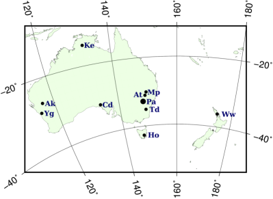
Figure 1: The LBA stations network. Station Hh (hartrao), 60 km north-west of Johannesburg, South Africa, is not shown.

Stations atca, ceduna and mopra were equipped with the LBA VLBI backend consisting of an Australia Telescope National Facility (ATNF) Data Acquisition System (DAS) with an Longe Baseline Array data recorder (LBADR) (Phillips et al., 2009). The ATNF DAS only allows two simultaneous intermediate frequencies (IFs): either 2 frequencies or 2 polarizations. For each of these IFs the input 64 MHz analog IF is digitally filtered to 2 contiguous 16 MHz bands. Stations atca and mopra were equipped with two LBDAR recorders, however because of hardware limitations, additional recorders could not be used for expanding frequency coverage, but could be used for recording both polarizations. Thus, the stations equipped with the ATNF backend could record two bands 32 MHz wide. This imposed a limitation on the frequency setup: spreading the frequencies too narrow would result in a degradation of group delay accuracy and spreading the frequencies too wide would results in group delay ambiguities with very narrow group delay ambiguities spacings. Our choice was to spread 32 MHz sub-bands over 256 MHz band that allowed us to determine group delay with uncertainly 123 ps when the signal to noise ratio is 10 and with ambiguity of 3.9125 ns.

Other stations were equipped with Mark-5 data acquisition terminals. Station ceduna was upgraded from the ATNF backend to Mark-5 in 2015 and used Mark-5 in the last three observing sessions. Stations equipped with Mark-5 recorded 256 MHz bandwidth, except tidbinbilla that prior 2016 was able to record only 128 MHz, and station askap that could record a single bandwidth 64 MHz, dual polarization. The stations equipped with Mark-5 recorded more 16 MHz wide frequency channels with 320 MHz wide spanned bandwidth that partly overlapped with the frequency channels recorded by the stations with the ATNF backend. In every experiment from 2 to 5 different setups were used, and these setups were changing from an experiment to experiment. Figure 2 as an example shows the frequency setup of v271i experiment. The versatility of the difx correlator (Deller et al., 2011) was exploited to cross-correlate the overlapping regions of such experiments. The heterogeneity of the available VLBI hardware made correlation more difficult but fortunately, did not introduce noticeable systematic errors in group delay. The most profound effect of this frequency allocation is ambiguities in group delay at baselines with stations with the ATNF backends.

The telescopes at NASA’s Deep Space Network (DNS) located at Tidbinbilla (Td), near Canberra, participated in the network, when available. These are Deep Space Station 34 (DSS-34, 34m, for v271h,j,m, and v441a), DSS-45 (34m, for v271a,b,l), and DSS-43 (70m, for v493a). Their primary mission is to support communication with spacecrafts but also support VLBI for celestial reference frame maintenance, navigation, and astronomy for limited amount of time. For LBA, usually short blocks of 3–5 hour were available during time not suited for deep space communication. Mark-5a system was used to record 8x16MHz channels for this series except v493a recorded 2x64MHz with LBA-DR. System temperatures at single-band 8GHz mode the are 22K, 20K, and 12K for DSS-45, DSS-34, and DSS-43, respectively Chang (2019). DSS-45 has been decommissioned in November 2016 after operation for 34 years.

Table 2: List of the LBA Calibrator Survey experiments. The first column shows the campaign segment, the second and third show the observing session and experiment ID, and the last segment shows the network of participating stations.

LCS–1	20080205_r	v254b	At-Cd-Ho-Mp-Pa
LCS–1	20080810_r	v271a	At-Cd-Ho-Mp-Pa-Td
LCS–1	20081128_r	v271b	At-Cd-Ho-Mp-Pa-Td
LCS–1	20090704_r	v271c	At-Cd-Ho-Mp-Pa
LCS–2	20091212_r	v271d	At-Cd-Ho-Mp-Pa
LCS–2	20100311_r	v271e	At-Cd-Ho-Mp-Pa
LCS–2	20100725_p	v271f	At-Cd-Ho-Mp-Pa
LCS–2	20101029_p	v271g	At-Cd-Mp-Pa
LCS–2	20110402_p	v271h	At-Cd-Ho-Hh-Ww-Td
LCS–2	20110723_p	v271i	Ak-At-Cd-Ho-Hh-Mp-Pa-Td-Ww
LCS–2	20111111_p	v271j	At-Cd-Ho-Hh-Mp-Td
LCS–2	20111112_p	v441a	At-Cd-Ho-Hh-Mp-Td
LCS–2	20120428_p	v271k	At-Cd-Ho-Hh-Mp-Pa-Ww-Yg
LCS–2	20130315_p	v271l	Ak-At-Cd-Ho-Hh-Mp-Pa-Ww-Td
LCS–2	20130615_p	v271m	At-Cd-Ho-Hh-Mp-Pa-Ww-Td
LCS–2	20140603_p	v493a	At-Cd-Ho-Hh-Mp-Pa-Td
LCS–2	20150407_p	v271n	At-Cd-Ho-Hh-Ke-Pa-Ww-Yg
LCS–2	20150929_q	v271o	Ak-At-Cd-Ho-Hh-Ke-Pa-Ww-Yg
LCS–2	20160628_q	v493c	Ak-At-Cd-Ke-Mp-Pa-Yg

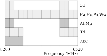
Figure 2: The frequency allocation in v271i experiment. The channel width is 16 MHz for all stations, except Ak, which has the channel width 64 MHz. Single polarization channels are shown with light-gray color and dual polarization channels are shown with dark-Gray color.

The Australia Telescope Compact Array (ATCA) consists of six 22 m antennas. Five of them can be phased up and record the signal from each individual telescope as a single element of the VLBI network. The position of the ATCA phase center can be set to any of the antenna positions. However, we exercised caution in using the phased ATCA since attempts to use the phased Westerbork array for astrometry revealed significant phase fluctuations in the past which rendered it highly problematic for precise astrometry (Sergei Pogrebenko, private communication, 2010). Therefore, we investigated the performance of the phase ATCA in a special 4 hour long test experiment that we ran on May 08, 2010. Stations atca, ceduna, hobart26, mopra, and parkes recorded the same frequency setup as in the LCS experiments. For the first 60 seconds of a 4 minute long scan the ATCA recorded signal from the single antenna at pad with ID W104 (see LCS1 paper for the nomenclature of ATCA pads), then it switched to the phased array with the phase center at the same pad and recorded for a further 90 second. Finally, ATCA switched back to recording the signal from a single station. In total, 232 scans of strong sources were recorded. The typical plots of the normalized uncalibrated fringe amplitude and fringe phase as a function of time within a scan are shown in Figure  3.

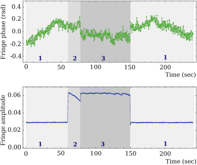
Figure 3: The fringe plot at atca/parkes, source J2225-0457 during vt10k test experiment. The upper plot shows fringe phase, the lower plot shows fringe amplitude. Light-gray area “1” denotes the interval when single ATCA station records. The dark-gray area “3” denotes the interval when the phased-array records. The medium-gray area “2” denotes the intermediate interval.

We see that for 18 seconds after switching to the phased-up mode the fringe amplitude is steadily drops by 15% and then suddenly returns back and stays stable within 2%. We consider this as transitional interval. The fringe phase does not show any change greater 0.01 rad just after switching back to the phased mode, but shows a sudden change in a range of 0.1–0.2 rad after the end of the transitional interval and immediately after switching from the phased to the single antenna record mode.

We computed average fringe phases, phase delay rates, group delays, and group delay rates by running the fringe fitting algorithm trough the same data three times. During the first processing run we masked out single antenna recording mode and the first 18 s of the phased recording mode keeping 72 s long data in each scan when ATCA recorded in the phased mode. During the second processing run we masked out the data when ATCA recorded in the phased mode. During the third run we processed first 60 s and last 90 s of each scan when ATCA recorded in the single antenna mode. We referred group delay and fringe phases to the same common epoch within a scan and formed their differences.

The differences in group delay between phased and single antenna recording modes at different baselines with ATCA are shown on Figure 4 with green color. The weighted root mean square (wrms) of the differences is 38 ps. For comparison, the differences in group delays computed using the first 60 seconds and last 90 seconds of a 4 minute long scan recorded at ATCA in the single antenna mode and referred to the same middle epoch are shown with blue color. The wrms of these differences is 59 ps. The differences in fringe phase between recording at ATCA with phased model and single antenna mode are shown in Figure 5. The wrms of phase differences is 0.12 rad.

We analyzed the dependence of differences versus elevation, azimuth and parallactic angle, but found no pattern. The uncalibrated averaged fringe amplitude at baselines to the ATCA data recorded as a phased array is a factor of 2.27 greater than the uncalibrated fringe amplitude with ATCA data recorded as a single antenna, which is within 2% of $\sqrt{5}$.

We found that phasing ATCA up does not introduce noticeable systematic errors in group delay and fringe phases. The differences in group delays is a factor of 1.5 less than the difference in group delay computed from two subset of data separated by 90 s. The differences in phases is the random noise with wrms is 0.12 rad, which corresponds to 0.6 mm. Therefore, we concluded that using of phased ATCA as an element of the VLBI network does not introduce systematic errors, but improves sensitivity of ATCA by a factor of 2.27. This was the first use of a phased array as an element of a VLBI network for absolute astrometry.

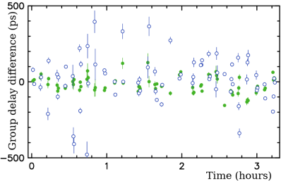
Figure 4: Differences in group delays from the same observations in test vt10k experiment. The solid green circles show the differences in group delay between ATCA phased-array and ATCA-single stations. The wrms of the differences is 38 ps. For comparison, the whole blue circles show the differences in group delay from first 60 sec and last 90 seconds of the integration interval.

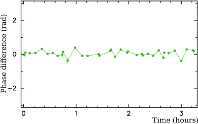
Figure 5: Differences in fringe phase delays between ATCA phased-array and ATCA-single recording from the same observations in test vt10k experiment. The wrms of the differences ins 0.12 rad.

2.2 Source selection

We selected for observations as target sources the objects that had previously been detected with single dish observations or with connected element interferometers with baselines 0.1–5 km. The input catalogues provided estimates of flux density at angular resolutions of 1–$100^{\prime\prime}$. The response of an interferometer to an extended source depends on its compactness and the size of the interferometer. The baseline projection lengths of the LCS network vary in a range of 5–300 M$\lambda$. That means the interferometer will be sensitive for emission from the compact components of milliarcsecond size. The response to extended emission with a size more than 1 mas at the longest baselines and 50 mas at the shortest baselines will be attenuated, and the interferometer will not detect signal from emission with size a more than a factor 2–5 beyond that level.

In order to maximize the number of detected sources, we have to select the targets with the highest compactness: the ratio of the correlated flux density at 5–300 M$\lambda$ to the total flux density. As a marker of high compactness, we initially used spectral index defined as $S\sim f^{+\alpha}$, where $f$ is the frequency. As a result of synchrotron self-absorption, the emission from the optically thick jet base that is morphologically referred to as the core of an AGN, has flat ($\alpha\approx 0$) or inverted spectrum ($\alpha>0$). The optically thick emission from an extended jet and extended radio-lobes that are a result of interaction of the jet with the surrounding interstellar medium usually has steep spectrum ($\alpha<1$). Therefore, one can expect the sources with flat spectrum, on average, will have a higher compactness, which has been confirmed with observations (e.g., Beasley et al., 2002).

Our source selection strategy gradually evolved for the course of the 8-yr long campaign, but all the time it was focused on selecting the sources with brightest correlated flux density. In the first three experiments we selected sources with spectral index $>-0.50$ from the quarter-Jansky survey (Jackson et al., 2002) brighter than 200 mJy. In following experiments we used several criteria for selecting the targets. In experiments v271c–v271m we selected the candidate sources brighter than 150 mJy with spectral index $>-0.55$ from the AT20G catalogue. In addition to that, we selected sources brighter 180 mJy and spectral index $>-0.55$ from the PMN catalogue (Griffith & Wright, 1993; Wright et al., 1994; Griffith et al., 1994; Condon et al., 1993; Tasker et al., 1994; Griffith et al., 1995; Wright et al., 1996). The PMN catalogue was derived from processing single-dish observations with parkes at 4.85 GHz, and it is complete at least to 50 mJy at declinations below $-37^{\circ}$. In v271k–v271m experiments we selected the sources brighter than 170 mJy and spectral index $>-0.55$ from the ATPMN catalogue (McConnell et al., 2012). The priority was given to sources with declinations $<-40^{\circ}$, although a small fraction of sources with declinations in the range [$-30^{\circ},-40^{\circ}$] were also observed. We should note here that we selected some sources from these pools and did not have intention to select all the sources.

However, an approach of selecting flat spectrum sources does not provide a good prediction for correlated flux density for the sources within 5–$7^{\circ}$ of the Galactic plane. The Galactic plane is crowded, and the chance of making an error in cross-matching the sources observed with instruments at different angular resolutions and poor positional accuracy is rather high. This will result in a gross mistake in the estimate of the spectral indices. Also, the density of galactic sources with flat spectrum, such as supernova remnants and ultra-compact H II regions is much higher within the Galactic plane. An attempt to observe flat spectrum sources in the Galactic plane by cross-matching the MGPS-2 catalogue at 843 MHz (Murphy et al., 2007) with other catalogues resulted in a detection rate of $\sim\!10\%$. To overcome this problem, we used another approach to find candidate sources in the Galactic plane: we analyzed an IR color-color diagram. Massaro et al. (2011) noticed that the blazars occupied a special zone in the color-color diagram 3.4–4.6 $\mu$m and 4.6–12 $\mu$m. We analyzed this dependence ourselves and delineated the zone that encompasses over 85% compact radio-loud AGNs from the cumulative VLBI catalogue Radio Fundamental Catalogue (RFC) (Petrov & Kovalev, in preparation). See section 4.2 in Schinzel et al. (2015) for detail. We tried an alternative approach: we selected all the sources within $5^{\circ}$ of the Galactic plane and declinations below $-40^{\circ}$ and flux density $>50$ mJy and left those that have cross-matches against IR WISE catalogue (Wright et al., 2010; Mainzer et al., 2011) within $30^{\prime\prime}$. Then we threw away sources that are beyond the zone of the 3.4–4.6 $\mu$m and 4.6–12 $\mu$m diagrams containing 85% radio loud AGNs. We observed the brightest sources from the remaining sample. The detection rate of this sample was 57%.

In addition to these selection methods, we observed in three experiments, v441a, v493a, and v493c, the flat spectrum sources brighter 10 mJy that were detected at 5 and 9 GHz by the Australia Telescope Compact Array (ATCA) within its error ellipse, i.e. 2–$5^{\prime}$, of unassociated $\gamma$-ray sources detected with Fermi mission (Abdo et al., 2010) that we found in a dedicated program (Petrov et al., 2013; Schinzel et al., 2015, 2017) focused in finding the most plausible radio counterparts of $\gamma$-ray source. Since radio-loud $\gamma$-ray AGNs tend to be very compact, the presence of a radio source detected with a connected interferometer within the error ellipse of a $\gamma$-ray object raises the probability of being detected with VLBI. Observing such sources firstly, fits the primary goal of the LCS program and secondly, allows us to find associations to Fermi objects that previously have been considered unassociated.

2.3 Scheduling

The experiment schedules were generated automatically with the program sur_sked in a sequence that minimizes the slewing time and obeys a number of constraints. Target sources were observed in three to four scans for 2 to 4 minutes long each, except weak candidates to Fermi associations that were observed for 5–10 minutes. VLBI experiments had a nominal duration of 24 hours. During each session, 80–100 target sources were observed. The minimum gap between consecutive observations of the same source was set to 2.5 hours. Station parkes was required to participate in each scan, since it is the most sensitive antenna of the array. After 1.5 hours of observing targets sources, a block of calibrator sources was inserted. These are the sources picked from the pool of known compact objects stronger 300 mJy. The block consists of 4 sources, with two of them observed at each station in the elevations in the range of 10–$30^{\circ}$ (30–$40^{\circ}$ for parkes that has the low elevation limit $31^{\circ}$) and two observed at elevations 55–$85^{\circ}$. The goal of these observations were: 1) to improve the estimate of the atmosphere path delay in zenith direction; 2) to connect the LCS catalogue to the accumulative catalogue of compact radio sources; 3) to use these sources as bandpass calibrators; and 4) to use these sources as amplitude calibrators for evaluation of gain corrections.

3 Data analysis

The antenna voltage was sampled with 2-bits with an aggregate bit rate from 256 to 1024 millions samples per second. The data analysis chain consist of 1) correlation that is performed at the dedicated facility, 2) post-correlation analysis that computes group delays and phase delay rates using the spectrum of cross-correlated data; 3) astrometric analysis that computes source positions, and 4) amplitude analysis that either produces source images or estimates of the correlated flux density at the specified range of the lengths of projected baselines.

3.1 Correlation and post-correlation analysis

The first four experiments were correlated with the Bonn Mark4 Correlator. The data from atca-104, ceduna, and mopra, originally recorded in LBADR format, were converted to Mark-5b format before correlation. Post-correlation analysis of these data was performed at the correlator using software program fourfit, the baseline-based fringe fit offered within the Haystack Observatory Package Software (hops) to estimate the residual group delay and phase delay rate. More detail about processing these experiments can be found in Petrov et al. (2011b).

The rest of the experiments were correlated with the difx software correlator (Deller et al., 2011) at the Curtin University and then by CSIRO. The output of the difx correlator was converted to FITS-IDI format and further processed with pima VLBI data analysis software (Petrov et al., 2011a). The correlator provided the time series of the auto- and cross-spectrum of the recorded signal with a spectral resolution 0.25 MHz and time resolution 0.25 s. Such a choice of correlation parameters allowed us to detect sources within several arcminutes of the pointing direction, i.e., everywhere within the primary beam of parkes radio telescope that has full with half maximum (FWHM) at 8.3 GHz close to $2^{\prime}$.

The post-correlator analysis chain includes the following steps:

• Coarse fringe fitting that is performed using an abridged grid of group delays and delay rates without further refinement. The goals of this step is to find at each baseline 10–15 observations with the highest signal to noise ratio (SNR) and detect failures at one or more IFs.

• Computation of a complex bandpass using the 12 observations with the highest SNR. The complex bandpass describes a distortion of the phase and amplitude of the recorded signal with respect to the signal that reached the antennas. We flagged at this step the IFs that either were not recorded or failed. We used 12 observations for redundancy in order to evaluate the statistics of a residual deviation of the phase and amplitude as a function of frequency from the ideal after applying the bandpass computed over the 12 observations using least squares. Large residuals triggered detailed investigation that in a case of a serious hardware failure resulted in flagging affected spectral channels.

• Fine fringe fitting that is performed with using the complex bandpass and the bandpass mask derived in the previous step. The preliminary value of the group delay and phase delay is found as the maximum element of the two-dimensional Fourier transform of the time series of cross-correlation spectrum sampled over time and frequency with a step 4 times finer over each dimension than the original data. The final value of the group delay and phase delay rate is adjusted from phases of the cross-correlation function (also known as fringe phases) as small corrections to the preliminary values using least squares. Phase residuals of the cross-correlation spectrum are analyzed and additive corrections to the a priori weights are computed on the basis of this analysis. The uncertainties of estimates of group delays are derived from uncertainties of fringe phases and additive weights corrections. The uncertainties of fringe phases depend on fringe amplitudes. The explicit expression can be found on page 233 of Thompson et al. (2017), equation 6.63.

• Computation of total group delays and phase delay rates. The group delays and phase delay rates derived at the previous step are corrections to the a priori delays and phase delay rates used during correlation. The mathematical model of the a priori group delay and phase delay rate used by the correlator is expanded over polynomials of the 5th order at 2 minute long intervals that cover the time range of a VLBI experiment. Using these coefficients, the a priori group delays and phase delay rates are computed to a common epoch within a scan for the event of arriving the wavefront at a reference station of a baseline. Using these a priori group delays and phase delay rates, the total group delays for that epoch are formed.

3.2 Astrometric analysis

Total group delay is the main observable for astrometric analysis. During further analysis, the a priori model of group delay, more sophisticated than that used for correlation, is computed, and the differences between observed and theoretical path delays are formed. The partial derivatives of this model over source coordinates, station positions, the Earth ordination parameters, atmosphere path delay in zenith direction, and clock function are also computed. Then corrections to those parameters are adjusted using least squares.

The frequency setup used for this campaign, selected due to hardware limitation (see as an example the setup for v271i segment in Figure 2) posed a challenge in data analysis. The Fourier transform over frequency over baselines with atca, ceduna, mopra in this example that uses LBDAR data acquisition system has strong secondary maxima (see Figure 6). The amplitude of the 2nd maximum is 0.98, the third maximum 0.93, and the fourth maximum 0.83 with respect of the global maximum. Due to the noise in data and remaining instrumental phase distortion, the fringe fitting process cannot reliably distinguish the primary and the secondary maxima, and as a result, group delay is determined with the ambiguity of $N\times 1/2.56\cdot 10^{8}\approx 3.9$ ns, where $N$ is a random integer number, typically in a range [-2,2].

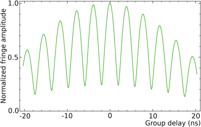
Figure 6: The normalized fringe amplitude as a function of group delay between stations that had LBDAR recording system. The fringe amplitude is divided by the amplitude at the global maximum.

At the first stage of the astrometric data analysis we processed the so-called narrow-band group delays derived as an arithmetic mean of group delays computed over each IF independently and estimated source positions using least squares. The dataset of narrow-band group delays was cleaned for outliers during the residual analysis procedure. The narrow-band delays do not have ambiguities, but are one order of magnitude less precise than group delays computed over the entire band. The estimated parameters at this stage are station positions and coordinates of target sources, as well as atmospheric path delays in zenith direction and clock function in a form of expansion over the B-spline basis. The contribution of the adjusted parameters to path delay computed using the narrow-band delays is substituted to the group delay residuals and then used for initial resolving group delay ambiguities. The procedure for group delay ambiguity resolution is described in detail in Petrov et al. (2011b).

After the group delay ambiguities are resolved, the dataset is cleaned for outliers in group delay. If necessary, the parametric model of clock is refined for incorporating discontinuities at specified epochs. Initial data weights were chosen to be reciprocal to the group delay uncertainty $\sigma_{g}$. Then the additive baseline-dependent weight corrections $a$ were computed for each observing session to make the ratio of the weighted sum of residuals be close to their mathematical expectation. These weights we used in the initial solution. The weights used in the final solution had a form

$$w=\frac{\displaystyle 1}{\displaystyle k\cdot\sqrt{\sigma_{g}^{2}+a^{2}+b^{2}}},$$ (1)

where $k$ is a multiplicative factor and $b$ an additive weight correction for taking into account mismodeled ionosphere contribution to group delay (see below). Such a clean dataset of group delays is used in further analysis.

The final LCS catalogue was derived in a single least square solution using all dual-band X/S (8.4/2.3 GHz) observations since 1980 through July 2018 under geodesy and astrometry programs that are publicly available and 19 LCS X-band experiments. The estimated parameters are split into three groups: global parameters that are adjusted for the entire dataset, local parameters that are specific for a given experiment, and segmented parameters that are specific for a time interval shorter than the observing session duration. The global estimated parameters are coordinates of all observed sources, positions and velocities of all observing stations, harmonic variations of station positions at annual, semi-annual, diurnal, and semi-diurnal frequencies, as well as B-spline coefficients that describe discontinuities and a non-linear motion of station caused by seismic activity. The local parameters are pole coordinates, UT1, and their first time derivative. The segmented parameters are clock function for all the stations, except the reference one, and residual atmosphere path delays in zenith direction.

For the course of the LCS campaign, a number of target sources were observed in follow-up VLBI experiments. We excluded these sources from the list of dual-band experiments in our LCS solution. The position of target sources were derived using only 8.3 GHz LCS data. Observations of these sources were later used for LCS catalogue error evaluation and computation of the weight correction factor $k$.

Since equations of electromagnetic wave propagation are invariant with respect to a rotation of the celestial coordinate system, as well as a translation and rotation of the terrestrial coordinate system, the system of equations has a rank deficiency and determines only a family of solutions. In order to define the solution from that family, we applied no-net-rotation constraints for source coordinates requiring the new positions of 212 so-called defining sources have no net-rotation with with respect to their positions in the ICRF1 catalogue (Ma et al., 1998). Similarly, we imposed the no-net-rotation and no-net-translation constraints on station positions and velocities.

3.3 Imaging analysis

We derived images of observed sources from one LCS experiment v271e that was run on March 2010 and used 5 LBA antennas. A list of 155 sources was observed in that experiment, and of them, 122 have been successfully detected, including 80 target sources and 42 troposphere calibrators. The expected theoretical thermal noise range is between 0.1 and 0.4 mJy/beam depending on the number of antennas and number of scans per source.

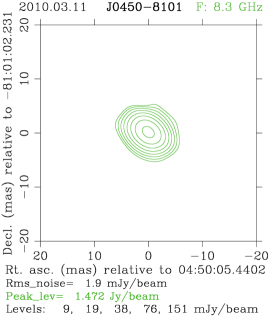
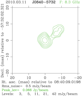
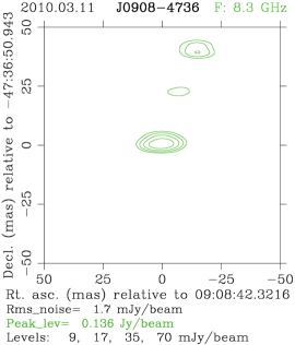
Figure 7: From left to right, contour plots for sources J0450$-$8101, J0840$-$5732, and J0908$-$4736 from LCS experiment v271e. The declination axis is towards up and the horizontal is towards left.

The correlated visibility data were processed using NRAO Astronomical Image Processing System (aips) software suite of programs (Greisen, 2003) independently from astrometric analysis. The data were read into AIPS together with tables containing system temperature information extracted from observing logs and antenna gain curves later used to calibrate the visibility amplitudes. When system temperature measurements during observations were not available, nominal values were used instead. Amplitude gain corrections in the cross-correlation spectra due to sampling have also been applied. Thereafter, the data inspection, initial editing and fringe fitting were done in the traditional manner using aips.

Fringe fitting in image mode was done independently from fringe fitting for the astrometry data analysis. We run fringe fitting with aips two times. The first run of fringe fitting was used before the bulk of the editing to find a preliminary approximation for the residual rates and delays. The estimates of group delay and phase delay rate were smoothed in time, and then used to calibrate the visibilities. The main editing of the visibility data was then done using this approximate calibration. Finally, a second run of fringe fitting using the edited data was used to refine the rate and delay calibration.

The overall amplitude gains were then further improved by self-calibrating five of the most compact and brightest calibrator sources and then using a CLEAN image of each of them as a model to determine the antenna gains that will make the visibility data for the chosen source/model conform as closely as possible to a point source. The derived gain corrections were averaged over all five sources an then applied to the remainder of sources.

After further inspection of the quality of the calibrated visibility data, the sources were then further self-calibrated in amplitude and phase using a CLEAN image of the source itself as a model. We made final CLEAN images using a weighting function of the visibilities in between uniform and natural weighting and using the square root of the statistical visibility weights. It was not possible to conclusively determine the basic source structure for a number of sources, and we did not attempt deconvolution or further self-calibration for such objects. The uv coverage for the LCS experiments is often poor and it is not possible to make satisfactory images for every detected source. In total, there were five target sources for which we were not able to produce an image using v271e data: J0413$-$5332, J2103$-$3058, J2107$-$4828, J2239$-$3609 and J2359$-$6054. In Figure 7 we show representative contour plots from imaging results obtained from the v271e session of the LCS.

In addition to imaging, the correlated flux density and FWHM source size were determined by fitting a simple Gaussian model of the emission directly to the visibilities by least-squares fitting (using the aips task UVFIT). The fitted values are listed in Table 3. Because of the limited, and sometimes highly elongated uv coverage, we did not attempt to characterize the source geometry beyond that of a mere estimate of the scale of the source structure from a simple circular Gaussian model. A circular Gaussian model was used, because it has a small number of parameters. The free parameters were the source position (x,y), the peak flux density and the FWHM of the Gaussian that fits the source image. Visibility plots and CLEAN images (where possible), were examined to make sure that a circular Gaussian model is reasonable and that the source is not a double for example.

(1)	(2)	(3)	(4)	(5)
		Jy	mas	mas
LCS J0049$-$5738	0047$-$579	1.411	4.91	-1.00
LCS J0058$-$5659	0056$-$572	0.942	3.89	-1.00
LCS J0109$-$6049	0107$-$610	0.420	8.94	-1.00
LCS J0124$-$5113	0122$-$514	0.171	4.10	-1.00
LCS J0236$-$6136	0235$-$618	0.291	2.77	-1.00
LCS J0314$-$5104	0312$-$512	0.181	2.81	-1.00
LCS J0335$-$5430	0334$-$546	0.560	8.24	-1.00

Table 3: The first 7 rows of the table with results of estimated source flux density and the FWHM of the Gaussian fit from the v271e observations. The estimated uncertainty on the flux densities are 10%. Fitted FWHM sizes are given with either its estimated 1$\sigma$ uncertainty, or the 3$\sigma$ upper limit. Columns: 1) source J2000 name; 2) IVS name; 3) flux density; 4) FWHM size; 5) FWHM size uncertainty (-1.00 if unavailable); This table is available in its entirety in machine-readable table datafile2 and Virtual Observatory (VO) forms in the online journal. A portion is shown here for guidance regarding its form and content.

For estimating the uncertainty of the FWHM of the Gaussian model, one approach would be to just take the statistical uncertainty calculated from the model fitting. However, since some residual antenna-dependent calibration errors are likely, the fitted FWHM size can be strongly correlated with the antenna amplitude gains, and the previous assumption may be violated. For this reason, we also estimated the uncertainties of estimated parameters by redoing the model fitting for all of the sources, but this time with the antenna amplitude gains added as free parameters. However, because of the small amount of data, the per-source and per-antenna gain corrections estimated this way are not always reliable, so we do not use the value of the FWHM size, but only the estimate of its uncertainty, which takes into account the correlation between the antenna gains and the fitted FWHM size. We found that the statistical uncertainties calculated from the model fitting are $\sim\!15$–20% larger when the antenna amplitude gains are added as free parameters.

To estimate more realistic uncertainties, in particular, to take into account the contribution of residual mis-calibration, we also used a Monte Carlo simulation to perturb randomly the antenna gains for a number of trials and fit the FWHM size. In the absence of reliable estimates of antenna gains, we just randomly changed them to get a distribution of the fitted FWHM size. We assume the antenna gains are accurate at a level of 10%. Therefore, we calculated the uncertainty of the fitted FWHM size from the Monte Carlo simulation that is still based on an assumed 10% uncertainty in the antenna gains. The Monte Carlo simulations were carried out using 10 sources with 12 trials for each source. In each of the trials we varied the antenna gains by a random amount, with the mean of the random gain variation being 0 and the standard deviation being 10%. Although the number of trials was small, it is enough to determine the scale of this contribution to the overall uncertainty in the FWHM size, and to show that it is not the dominant contribution.

The estimated uncertainties for the FWHM size from the Monte Carlo simulations were always $<a$, the minimum measurable size in the visibility plane given by Lovell et al. (2000), determined as

$$a<240\,\frac{\displaystyle\sqrt{N/S}}{\displaystyle U},$$ (2)

where $a$ is in units of milliarcsecond, $N$ is the integrated rms noise of the observations in Janskys and $U$ is the maximum baseline length in units of M$\lambda$. Expressed in terms of a uniformly weighted beam size, Equation 2 can be written as

$$a<1.8\sqrt{N/S}\times\theta_{\rm beamsize},$$ (3)

where unites for $a$ and $\theta$ are milliarcseconds.

Due to the poor uv-coverage for these observations, a reliable estimate of the beamsize could not always be obtained and thus, we calculated the beamsize as the geometric mean of the beam major and minor axes of the CLEAN beam. The fitted value of the beamsize for the v271e observations is $\sim 4$ milliarcseconds.

From the error calculations described above, the maximum obtained value of the uncertainty were always $\leq 1/4$ of the beamsize. Due to the limited uv coverage and the simple approximation of a circular model, we used 1/4 of the beamsize as a very conservative estimate of the uncertainty for all of the sources. From the Monte Carlo simulations the uncertainty on the flux densities were 10%.

3.4 Non-imaging analysis

As we see in Figure 7, the quality of images is not great because of scarcity of data and a poor $uv$-coverage. Direct imaging either produces maps with a dynamic range around 1:100 with a high chance of an imaging artefact to be unnoticed or, if to pursue elimination of artefacts aggressively, the images will be close to a point-source or a single component Gaussian.

Recognizing these challenges, we processed the entire datasets by fitting a simplified source model to calibrated visibilities. We limited our analysis to evaluation of the median correlated flux density estimates in three ranges of lengths of the baseline projections onto the plane tangential to the source, without inversion of calibrated visibility data using the same technique as we used for processing first 4 LCS experiments (Petrov et al., 2011b). A reader is referred to this publication for detail. Here we outline the procedure.

At the first step, we analyze system temperatures, remove outliers, evaluate the radiative atmosphere temperature, compute receiver temperatures, interpolate them for restoring missing data, and generate a cleaned dataset of system temperatures. Dividing it by the a priori elevation-dependent antenna gain, we get the a priori system equivalent flux density (SEFD).

At the second step, we estimate station-dependent multiplicative gain corrections to calibrated fringe amplitudes of calibrator sources with least squares by using a number of sources with known 8 GHz images that can be found in the Astrogeo VLBI FITS image database that we maintain. During this procedure, we iteratively exclude those images which resulted in large residuals. Due to variability, the flux density of some individual sources may raise or decline, but the average flux density of a source sample is expected to be more stable than the flux density of individual objects.

At the third step, we apply adjusted SEFDs and compute the correlated flux densities of target sources. Then we sort the fringe amplitude over baseline projection lengths and compute median estimates of the correlated flux density in three ranges: 0–10 M$\lambda$ ($<360$ km), 10–40 M$\lambda$ (360-1440 km) and 40–300 M$\lambda$ (1400–10800 km). These parameters characterize the strength of a source, and it has to be accounted for scheduling the observations. The accuracy of this procedure is estimated at a level of 20% judging on residuals of gain adjustments.

The list of 49915 estimates of correlated flux densities from individual observations of 1100 target sources and 368 calibrator sources is presented in the machine-readable table datafile4. The table contains the following information: source name, date of observations, baseline name, $u$- and $v$- projections of the baseline vector, the correlated flux density and their formal uncertainty, the signal to noise ratio, the instants system equivalent flux density for this observation, and the observing session code.

4 Error analysis

Single-band group delays are affected by the contribution of the ionosphere. Considering the ionosphere as a thin shell at a certain height above the Earth surface (typically 450 km), the group delay can be expressed as

$$\tau_{\rm iono}=\frac{\displaystyle\alpha}{\displaystyle f^{2}_{\mbox{eff}}}\>\mbox{TEC}\>\frac{\displaystyle 1}{\displaystyle\cos{\beta}},$$ (4)

where $f_{\mbox{eff}}$ is the effective frequency, $\beta$ is the zenith angle at the ionosphere piercing point, TEC is the total electron contents in the zenith direction at the ionosphere piercing point, and $\alpha$ is a constant (see Sovers et al. (1998) for detail). We have computed the a priori ionosphere contribution to group path delay using TEC maps from analysis of Global Navigation Satellite System (GNSS) observations. Specifically, we used CODE TEC time series (Schaer, 1999) with a resolution of $5^{\circ}\times 2.5^{\circ}\times 1^{h}$ ($5^{\circ}\times 2.5^{\circ}\times 2^{h}$ before December 19, 2013).

The TEC model from GNSS observation is an approximation, and the accuracy of a priori $\tau_{\rm iono}$ from such a model is noticeably lower than the accuracy of $\tau_{\rm iono}$ computed from the linear combination of group delays at X and S (or X and C) bands from dual-band observations. The errors of $\tau_{\rm iono}$ from such observations is at level of several picoseconds according to Hawarey et al. (2005). We consider the contribution of mismodeled ionospheric path delay as the dominating source of systematic errors and, therefore, we investigated it in detail.

We used the global dataset of VLBI observations after July 01, 1998 for investigation of the residual ionospheric contribution to group delay after applying the a priori path delay delay derived from CODE global TEC maps. For each dual-band observing sessions, we decompose the slant ionospheric path delay from X/S observations at the product of the path delay in zenith direction and the mapping function, the ratio of the ionospheric path delay in a given elevation to the ionospheric path delay in zenith direction. Then we computed the rms of the total $\tau_{\rm iono}$ in zenith direction from CODE global TEC maps, $\sigma_{t}$, and the rms of the differences in $\tau_{\rm iono}$ in zenith direction derived using the CODE global TEC maps and the dual-band X/S group delays, $\sigma_{r}$. The ratio of these two statistics, variance admittance $A=\frac{\sigma^{2}_{r}}{\sigma^{2}_{t}}$, is a measure of the model goodness. Assuming $A$ is stable in time, we can predict, unknown to us, statistics of $\sigma^{2}_{r}$ for single-band observations using $\sigma^{2}_{t}$ that we can compute from the TEC model. We derived time series of parameter $A$ from analysis of dual-band VLBI observations after July 01, 1998.

Further analysis showed that parameter $A$ is not stable with time. Since $A$ is computed as a ratio of variances, we sought an empirical regression models where $A$ enters as a multiplicative factor. We computed the global total electron content (GTEC) by averaging the TEC over the sphere. As it was show by Afraimovich et al. (2008), such a parameter characterizes the global state of the ionosphere. Figure 8 shows the dependence of $A$ on GTEC. We represent this dependence with a broken linear function with A=0.6 at GTEC=7.0, A=0.35 at GTEC=20.0 and A=0.25 at GTEC=60.0.

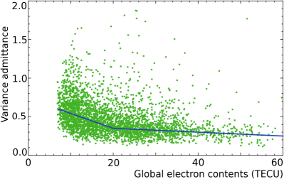
Figure 8: The dependence of the variance admittance factor $A$ on the global total electron contents. The so-called TEC units ($10^{16}$ electrons over zenith direction) are used for GTEC.

Using this dependence, we computed the GTEC for a given experiment, averaged it over the period of the experiment duration, computed parameter $A$ using the linear regression, computed the time series of the ionospheric contribution from the TEC model for each station of a baseline, and then computed the variances of the mismodeled contribution of the ionosphere to group delay in zenith direction for the first and second station of a baseline, $\mathop{\rm Cov}\nolimits_{11}$ and $\mathop{\rm Cov}\nolimits_{22}$, as well as their covariances $\mathop{\rm Cov}\nolimits_{12}$. Then for each observation we computed the predicted rms of the mismodeled ionospheric contribution as

$$b=A\sqrt{\mathop{\rm Cov}\nolimits_{11}^{2}\,M_{1}^{2}(e)-2\mathop{\rm Cov}\nolimits_{12}\,M_{1}(e)\,M_{2}(e)+\mathop{\rm Cov}\nolimits_{22}^{2}\,M_{2}^{2}(e)},$$ (5)

where $M_{1}(e)$ and $M_{2}(e)$ are the mapping function of the ionospheric path delay. These parameters $b$ were used for weight corrections in expression 1.

Parameter $A$ varied from 0.35 to 0.59 with a mean of 0.48 for the LCS campaign. This means that applying the ionospheric contribution from the CODE TEC maps, we reduce the variance of the total contribution by a factor of 2, and the mismodeled part of the contribution is accounted in inflating uncertainty of group delay. The known deficiency of this approach is that first, the regression dependence of parameter on $A$ on GTEC is rather coarse, and second, the correlations between residual ionospheric contributions are neglected.

For a check of the contribution of remaining systematic errors, we compared our source positions derived from X-band only LCS experiments with results of dual-band observations that included some LCS target sources. In 2017, the SOuthern Astrometry Program (SOAP) of dual-band follow-up observations at the Hh-Ho-Ke-Yg-Wa-Ww-Pa network at 2.3/8.4 GHz commenced. The goal of the program is to improve the positions of the bright sources with declinations below $-45^{\circ}$. By August 2018, 10 twenty-hour experiments were observed. parkes station participated in two of them. The sources as weak as 70 mJy were observed in experiments with parkes, 2–3 scans per sources, and objects brighter than 250 mJy were observed in other experiments, 8–10 scans per source. These experiments were made with the so-called geodetic frequency setup: 6 IFs of 16 MHz wide were spanned between 2.200 and 2.304 GHz (S-band) and 10 IFs of 16 MHz wide were spanned between 8.198 and 8.950 GHz (X-band). Group delays were computed for X and S band separately, and the ionosphere-free combinations of group delays were formed. At the moment of writing, the program has not finished, and a detailed analysis will be presented in the future upon completion of the program. Meanwhile, we use these 10 experiments to compare results and assess the errors.

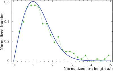
Figure 9: The distribution of the normalized arc lengths between LCS X-band only positions of 269 sources and their X/S positions from the follow-up campaigns (Green dots). For comparison, the Rayleigh distribution with $\sigma=1$ parameter is shown with a blue line.

We ran a global reference solution using all dual-band X/S observations of the LCS target sources including the SOAP observations and excluding LCS observations. The reference and the LCS solutions differed 1) in the list of sessions that were used in the solutions and 2) in treatment of the ionosphere. The reference solution used ionosphere-free linear combinations of S and X-band observables, while the LCS solution used X-band only group delays with the ionosphere contribution derived from CODE TEC maps applied during data reduction. The reference solution used weights according to equation 1 with k=1 and b=0.

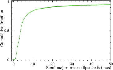
Figure 10: The cumulative distribution of the LCS position errors.

We have compared the positions of 373 LCS target sources that are common with the reference solution. We did not find any outlier exceeding 20 mas that can be caused by errors in group delay ambiguity resolution. That means that all observations with unreliable ambiguity resolution were correctly flagged out and did not degrade the solution. At the same time, we found that the arc lengths divided by the their uncertainties, so-called normalized arcs, were larger than expected with the mean value 1.89. We attributed this discrepancy to the underestimation of errors of LCS observations. To alleviate this underestimation, we varied the multiplicative factor $k$ in expression 1 in such a way the distribution of normalized arcs be as close to the Rayleigh distribution with $\sigma=1$ as possible. We found that when the LCS observations are re-weighted with parameter $k=1.80$ in equation 1, the distribution of normalized arcs over 269 sources that have at least 16 observations is the closest to the Rayleigh distribution (see Figure 9). The mean arc length is 3.4 mas and the median value is 2.5 mas. The cumulative distribution of the final LCS position errors is shown in Figure 10.

5 The catalogue

The first 8 rows of the LCS catalogue are presented in Table 4. The catalogue presents source positions, position uncertainties, the number of used observations, flux densities in three ranges of baseline projection lengths, and their formal uncertainties. In total, the catalogue has 1100 entries. The median semi-major error ellipse axes of reported positions is 3.6 mas. The flux densities are in a range from 3 mJy to 2.5 Jy, with the median 102 mJy. For completeness, the list of 405 sources that have been observed, but not detected is given in the machine-readable table datafile3. The flux densities of such sources turned out to be below the detection limit of baselines parkes/atca, parkes/hobart26, parkes/ceduna that is typically 6–8 mJy.

(1)	(2)	(3)	(4)	(5)	(6)	(7)	(8)	(9)	(10)	(11)	(12)	(13)	(14)
		hh mm ss.fffff	${}^{\circ}\hskip 10.00002pt{}^{\prime}\hskip 10.00002pt{}^{\prime\prime}\hphantom{aaa}$	mas	mas			Jy	Jy	Jy	Jy	Jy	Jy
LCS J0001$-$4155	2358$-$422	00 01 32.75494	$-$41 55 25.3367	215.1	92.3	-0.904	5	0.008	0.007	-1.0	0.001	0.002	-1.0
LCS J0002$-$6726	2359$-$677	00 02 15.19280	$-$67 26 53.4337	89.6	32.8	0.553	5	0.006	0.007	-1.0	0.001	0.001	-1.0
LCS J0002$-$5621	0000$-$566	00 02 53.46830	$-$56 21 10.7831	23.8	9.3	0.421	8	0.172	0.052	0.141	0.013	0.012	0.031
LCS J0003$-$5444	0000$-$550	00 03 10.63084	$-$54 44 55.9923	42.1	10.7	-0.112	9	0.006	0.006	-1.0	0.001	0.001	-1.0
LCS J0003$-$5247	0000$-$530	00 03 19.60042	$-$52 47 27.2834	39.0	18.5	-0.291	8	0.013	0.014	-1.0	0.002	0.002	-1.0
LCS J0004$-$4345	0001$-$440	00 04 07.25762	$-$43 45 10.1469	4.0	3.0	0.163	44	0.188	0.205	0.214	0.030	0.024	0.046
LCS J0004$-$5254	0001$-$531	00 04 14.01314	$-$52 54 58.7099	8.8	3.7	0.039	36	0.027	0.027	0.018	0.002	0.003	0.003

Table 4: The first 7 rows of the LCS catalogue. Columns: (1) source ID; (2) alternative source name; (3) J2000 right ascension; (4) J2000 declination; (5) uncertainty in right ascension without $\cos\delta$ factor; (6) uncertainty in declination; (7) correlation between right ascension and declination estimates; (8) the number of observations used in the solution; (9) the median correlated flux density at 8.3 GHz at baseline projection lengths in a range 0–10 M$\lambda$; (10) the median correlated flux density at baseline projection lengths in a range 10–40 M$\lambda$; (11) the median correlated flux density at baseline projection lengths in a range 40–300 M$\lambda$; 12) the median uncertainty of the correlated flux density at baseline projection lengths in a range 0–10 M$\lambda$; (13) the median uncertainty of the correlated flux density at baseline projection lengths in a range 10–40 M$\lambda$; (14) the median uncertainty of the correlated flux density at baseline projection lengths in a range 40–300 M$\lambda$. This table is available in its entirety in machine-readable table datafile1 and Virtual Observatory (VO) forms in the online journal. A portion is shown here for guidance regarding its form and content.

The distribution of LCS sources on the sky is shown in Figure 11. The distribution is rather uniform and does not have avoidance zones. For comparison, the sources known priori the LCS campaign are shown with blue color.

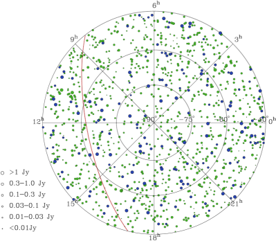
Figure 11: The sky distribution of compact radio sources at the Southern Hemisphere at 8.3 GHz. Blue light color denotes 186 sources with declinations $<-40^{\circ}$ with VLBI positions known prior the LCS program. Green dark color denotes 1100 sources detected in LCS program. Red line shows the Galactic plane.

6 Discussion

The median position uncertainty, 3.6 mas, cannot be called the VLBI state of the art nowadays. There are four factors that played the role. First, the contribution of the ionosphere cannot be computed using GNSS TEC models with the same level of accuracy as using simultaneous dual-band observations. Second, the scale of the network, less than 1700 km for the most observations degraded the sensitivity of observations to source positions, since the source position uncertainty is reciprocal to the baseline length. Station hartrao participated in less than 25% observations due to scheduling constraints. Third, the spanned bandwidth was limited to 320 MHz, compare with 720 MHz typically used in geodetic VLBI. Positional uncertainty is approximately reciprocal to the spanned bandwidth. Fourth, observed sources were rather week: 25% of target sources are weaker than 46 mJy.

Nevertheless, position accuracy of several milliarcseconds is sufficient for phase referencing. Figure 12 shows the probability of finding a phase calibrator brighter than 30 mJy within $2^{\circ}$ of any target with $\delta<-40^{\circ}$. For 88% of the area, such a calibrator can be found. Information about flux densities of detected sources and the upper limits for undetected sources greatly facilitates future follow-up observing programs focused on improvement of source positions.

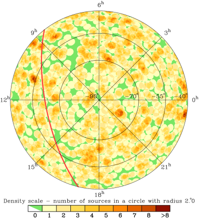
Figure 12: The sky density of calibrator sources at 8.3 GHz in the zone with declinations $<-40^{\circ}$ defined as the number of compact sources with flux density $>30$ mJy in a circle of $2^{\circ}$ radius. The Galactic plane is shown with the red line.

Among the 1100 LCS sources, there are 725 counterparts with Gaia DR2 (Lindegren et al., 2018) with the probability of false detection below 0.0002. See Petrov & Kovalev (2017a) for detail of the VLBI and Gaia association procedure. Petrov et al. (2019) showed that comparison of over 9,000 matched VLBI/Gaia sources reveled that 9% have statistically significant offsets at the level exceeding $4\sigma$. They presented extensive arguments showing that these offsets are real and are a manifestation of the presence of optical jets that affect the positions of optic centroid reported by Gaia. The LCS dataset has 53 (7.2%) outliers with an arc length exceeding $4\sigma$. The lower fraction of outliers is explained by worse position accuracy. These outliers were excluded from further analysis, since they do not characterize catalogue errors. The median arc length of position differences is 3.2 mas, while the median semi-major error ellipse axes of LCS positions of matched sources is 3.3 mas and the median semi-major error ellipse of Gaia positions of matched sources is 0.3 mas. This comparison demonstrates that the median of the differences between LCS and Gaia positions is very close to the reported median of the LCS semi-major error axis.

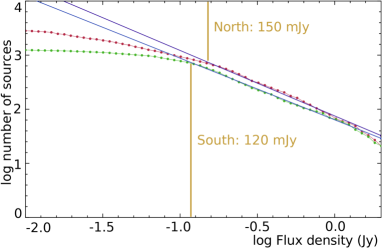
Figure 13: The log N – log S diagram for the LCS catalogue (low green line) using only the sources with $\delta<-40^{\circ}$. The upper red line shows a similar diagram for the sources with $\delta>+40^{\circ}$ at 8 GHz observed under other programs.

For analysis of LCS completeness we computed the so-called log N – log S diagram — the dependence of the logarithm of the number of sources on the logarithm of the total flux density recovered from VLBI observations. The dependence is approximated by a straight line within the range of flux densities that the catalogue is considered complete. With a decrease of flux densities, at some point the diagram deviates from a straight line. This point is considered the limit below which the catalogue is incomplete. The diagram in Figure 13 shows the completeness level of the LCS subsample at $\delta<-40^{\circ}$ drops below 95% at flux densities 120 mJy.

For comparison, we computed a similar diagram for the Northern Hemisphere at declinations $>+40^{\circ}$ using the Radio Fundamental Catalogue. The Northern Hemisphere catalogue has more weak sources, but surprisingly, its completeness drops below 95% level at flux densities 150 mJy. At the same time, the Northern Hemisphere catalogue has 23% more sources. One explanation is the total number of sources in the Southern Hemisphere is indeed $\sim\!20$% less due to a large scale fluctuation of the source distribution over the sky. Another explanation is a selection bias. The parent catalogue of the LCS is the AT20G at 20 GHz, while the parent catalogues of the Northern Hemisphere sources were observed at lower frequencies: 5–8 GHz. Selecting sources based on their emission at 20 GHz may result in omitting the objects with falling spectrum. The log N – log S dependencies for southern and Northern Hemispheres are almost parallel in a range of 0.15–0.65 Jy. If we accept the hypothesis that selecting candidate sources based on AT20G catalogue causes a bias, we have to admit that using AT20G as a parent sample we lose sources as bright as 0.5 Jy, which is difficult to explain. We think the problem of completeness of the LCS is still open, and more observations are needed in order to resolve it.

7 Compact and extended emission in a sub-sample of compact sources from AT20G

Of a sub-sample of 907 AT20G sources observed in the LCS campaign, 839 or 93% were detected. As noted by Chhetri et al. (2013), most of these AT20G sources are already known to be compact on scales of $\sim 0.15^{\prime\prime}$ at high frequencies.

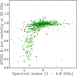
Figure 14: The ratio of the flux density at the 6 km long ATCA baseline to the flux density at short baselines from AT20G observations at 20 GHz (adapted from Figure 7 of Chhetri et al. (2013)).

Figure 14 plots the 6-km visibilities (defined as the ratio of the 20 GHz flux density on 6 km long baselines to the flux density at short baselines of 30–60 m; see Chhetri et al. (2013) for details) for the subsample of AT20G sources observed in the LCS campaign that also have 8.4 GHz flux density measurements in the AT20G catalogue. The red squares in this figure show local AT20G galaxies from the study by Sadler et al. (2014). Compact flat-spectrum AGN lie in the upper right quadrant and compact steep-spectrum (CSS) sources in the upper left, while the sources in the lower left quadrant are radio AGN with extended emission (mainly FR-1 radio galaxies) and angular sizes larger than 150 mas.

Figure 15 shows a similar plot where the compactness on much smaller scales is estimated by using the ratio of the flux density derived from VLBI observations at 8.3 GHz to the total flux density at 8.4 GHz from the AT20G observations. The majority of the flat-spectrum AT20G sources, while still detected on VLBI baselines, are now resolved at 10–40 M$\lambda$, which corresponds to 5–20 mas angular size. The sources with spectral index steeper than -0.5 show systematically lower compactness than the sources with flat radio spectra. The majority of VLBI non-detections (65 out of 68) are AT20G sources with steep radio spectra.

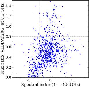
Figure 15: The ratio of the flux density from LCS at 8.3 GHz to the total flux density at 8.4 GHz from AT20G observations. The triangles show upper limits for the sources that were undetected on VLBI baselines.

The sub-sample of AT20G sources observed in the LCS is not complete, and further analysis is outside the scope of this paper. The compactness plots are shown here to demonstrate the potential of the LCS dataset, and a detailed analysis will be presented in a future paper.

8 Summary

The LCS VLBI observing program has provided positions of 1100 compact radio sources at declinations below $-30^{\circ}$ with accuracies at a milliarcsecond level and estimates of flux density at 8.3 GHz. As a result, the number of compact radio sources south of declination $-40\degr$ which have measured VLBI correlated flux densities and positions known to milliarcsecond accuracy has increased by a factor of 6.4. A dense grid of calibrator sources with precisely known positions is important for a number of applications, in particular for support of ALMA observations. The internal LCS test based on the log N – log S diagram shows it is complete at a 95% level for sources brighter than 120 mJy. At the same time, comparing the LCS with the Northern Hemisphere catalogue, we found a $\sim\!20$% difference in the source count. The LCS may have a deficiency of $\sim\!20$% sources because of using AT20G as a parent sample. It is yet to be resolved whether using high-frequency parent catalogue results in a systematic loss of sources with falling spectrum. The LCS catalogue is the Southern Hemisphere counterpart of the VLBA Calibrator Survey. The major outcome of this campaign is elimination of the hemisphere bias that the VLBI catalogues suffered in the past. However, technical limitations of the Southern Hemisphere telescopes provided position accuracy one order of magnitude worse than the accuracy of similar catalogues in the Northern Hemisphere. Future observations will target LCS sources for improvement of their positions, and the first such follow-up observing campaign started in 2017.

References

- Abdo et al. (2010) Abdo A. A., et al., 2010, ApJS, 188, 405
- Afraimovich et al. (2008) Afraimovich E. L., Astafyeva E. I., Oinats A. V., Yasukevich Y. V., Zhivetiev I. V., 2008, Annales Geophysicae, 26, 335
- Beasley et al. (2002) Beasley A. J., Gordon D., Peck A. B., Petrov L., MacMillan D. S., Fomalont E. B., Ma C., 2002, ApJS, 141, 13
- Chang (2019) Chang C., 2019, JPL Technilcal memorandum, 810–005
- Chhetri et al. (2013) Chhetri R., Ekers R. D., Jones P. A., Ricci R., 2013, MNRAS, 434, 956
- Condon et al. (1993) Condon J. J., Griffith M. R., Wright A. E., 1993, AJ, 106, 1095
- Condon et al. (2017) Condon J. J., Darling J., Kovalev Y. Y., Petrov L., 2017, ApJ, 834, 184
- Deller et al. (2011) Deller A. T., et al., 2011, PASP, 123, 275
- Fomalont et al. (2003) Fomalont E. B., Petrov L., MacMillan D. S., Gordon D., Ma C., 2003, AJ, 126, 2562
- Gordon et al. (2016) Gordon D., et al., 2016, AJ, 151, 154
- Greisen (2003) Greisen E. W., 2003, in Heck A., ed., Astrophysics and Space Science Library Vol. 285, Information Handling in Astronomy - Historical Vistas. p. 109, doi:10.1007/0-306-48080-8_7
- Griffith & Wright (1993) Griffith M. R., Wright A. E., 1993, AJ, 105, 1666
- Griffith et al. (1994) Griffith M. R., Wright A. E., Burke B. F., Ekers R. D., 1994, ApJS, 90, 179
- Griffith et al. (1995) Griffith M. R., Wright A. E., Burke B. F., Ekers R. D., 1995, ApJS, 97, 347
- Hawarey et al. (2005) Hawarey M., Hobiger T., Schuh H., 2005, Geophys. Res. Lett., 32, L11304
- Immer et al. (2011) Immer K., et al., 2011, ApJS, 194, 25
- Jackson et al. (2002) Jackson C. A., Wall J. V., Shaver P. A., Kellermann K. I., Hook I. M., Hawkins M. R. S., 2002, A&A, 386, 97
- Kovalev et al. (2007) Kovalev Y. Y., Petrov L., Fomalont E. B., Gordon D., 2007, AJ, 133, 1236
- Kovalev et al. (2017) Kovalev Y. Y., Petrov L., Plavin A. V., 2017, A&A, 598, L1
- Lindegren et al. (2016) Lindegren L., et al., 2016, A&A, 595, A4
- Lindegren et al. (2018) Lindegren L., et al., 2018, A&A, 616, A2
- Lovell et al. (2000) Lovell J. E. J., et al., 2000, in Hirabayashi H., Edwards P. G., Murphy D. W., eds, Astrophysical Phenomena Revealed by Space VLBI. pp 183–188
- Ma et al. (1998) Ma C., et al., 1998, AJ, 116, 516
- Mainzer et al. (2011) Mainzer A., et al., 2011, ApJ, 731, 53
- Massaro et al. (2011) Massaro F., D’Abrusco R., Ajello M., Grindlay J. E., Smith H. A., 2011, ApJ, 740, L48
- Matveenko et al. (1965) Matveenko L. I., Kardashev N.-S., Sholomitskii G.-B., 1965, Soviet Radiophys., 461, 461
- McConnell et al. (2012) McConnell D., Sadler E. M., Murphy T., Ekers R. D., 2012, MNRAS, 422, 1527
- Mignard et al. (2016) Mignard F., et al., 2016, A&A, 595, A5
- Murphy et al. (2007) Murphy T., Mauch T., Green A., Hunstead R. W., Piestrzynska B., Kels A. P., Sztajer P., 2007, MNRAS, 382, 382
- Murphy et al. (2010) Murphy T., et al., 2010, MNRAS, 402, 2403
- Napier et al. (1994) Napier P. J., Bagri D. S., Clark B. G., Rogers A. E. E., Romney J. D., Thompson A. R., Walker R. C., 1994, IEEE Proceedings, 82, 658
- Petrov (2011) Petrov L., 2011, AJ, 142, 105
- Petrov (2013) Petrov L., 2013, AJ, 146, 5
- Petrov (2016) Petrov L., 2016, preprint, (arXiv:1610.04951)
- Petrov & Kovalev (2017a) Petrov L., Kovalev Y. Y., 2017a, MNRAS, 467, L71
- Petrov & Kovalev (2017b) Petrov L., Kovalev Y. Y., 2017b, MNRAS, 471, 3775
- Petrov & Taylor (2011) Petrov L., Taylor G. B., 2011, AJ, 142, 89
- Petrov et al. (2005) Petrov L., Kovalev Y. Y., Fomalont E. B., Gordon D., 2005, AJ, 129, 1163
- Petrov et al. (2006) Petrov L., Kovalev Y. Y., Fomalont E. B., Gordon D., 2006, AJ, 131, 1872
- Petrov et al. (2008) Petrov L., Kovalev Y. Y., Fomalont E. B., Gordon D., 2008, AJ, 136, 580
- Petrov et al. (2011a) Petrov L., Kovalev Y. Y., Fomalont E. B., Gordon D., 2011a, AJ, 142, 35
- Petrov et al. (2011b) Petrov L., Phillips C., Bertarini A., Murphy T., Sadler E. M., 2011b, MNRAS, 414, 2528
- Petrov et al. (2013) Petrov L., Mahony E. K., Edwards P. G., Sadler E. M., Schinzel F. K., McConnell D., 2013, MNRAS, 432, 1294
- Petrov et al. (2019) Petrov L., Kovalev Y. Y., Plavin A. V., 2019, MNRAS, 482, 3023
- Phillips et al. (2009) Phillips C., Tzioumis T., Tingay S., Stevens J., Lovell J., Amy S., West C., Dodson R., 2009, in 8th International e-VLBI Workshop. p. 99
- Plavin et al. (2019) Plavin A. V., Kovalev Y. Y., Petrov L. Y., 2019, ApJ, 871, 143
- Sadler et al. (2014) Sadler E. M., Ekers R. D., Mahony E. K., Mauch T., Murphy T., 2014, MNRAS, 438, 796
- Schaer (1999) Schaer S., 1999, Geod.-Geophys. Arb. Schweiz, Vol. 59,, 59
- Schinzel et al. (2015) Schinzel F. K., Petrov L., Taylor G. B., Mahony E. K., Edwards P. G., Kovalev Y. Y., 2015, ApJS, 217, 4
- Schinzel et al. (2017) Schinzel F. K., Petrov L., Taylor G. B., Edwards P. G., 2017, ApJ, 838, 139
- Sovers et al. (1998) Sovers O. J., Fanselow J. L., Jacobs C. S., 1998, Reviews of Modern Physics, 70, 1393
- Tasker et al. (1994) Tasker N. J., Condon J. J., Wright A. E., Griffith M. R., 1994, AJ, 107, 2115
- Thompson et al. (2017) Thompson A. R., Moran J. M., Swenson Jr. G. W., 2017, Interferometry and Synthesis in Radio Astronomy, 3rd Edition. Springer, doi:10.1007/978-3-319-44431-4
- Wright et al. (1994) Wright A. E., Griffith M. R., Burke B. F., Ekers R. D., 1994, ApJS, 91, 111
- Wright et al. (1996) Wright A. E., Griffith M. R., Hunt A. J., Troup E., Burke B. F., Ekers R. D., 1996, ApJS, 103, 145
- Wright et al. (2010) Wright E. L., et al., 2010, AJ, 140, 1868