Matching Conditions and High-Re Anomalies in Hydrodynamic Turbulence.

Abstract

Direct transition from low Reynolds number ”weak” Gaussian turbulence to fully developed “strong” turbulence at a critical Reynolds number $R^{tr}_{\lambda}\approx 8.91$ has recently been theoretically predicted and tested in high resolution numerical simulations of V. Yakhot & D. A. Donzis, Phys. Rev. Lett. 119, 044501 (2017) & PhysicaD, 384-385, 12 (2018) on an example of a flow excited by a Gaussian random force. The matching between the low-Reynolds number Gaussian asymptotic ($Re<<Re^{tr}$) and the multi-scaling one, dominating the high-Re limit ($Re>>Re^{tr}$), led to closed approximate equation for exponents of moments of derivatives in a good agreement with experimental data. In this paper we study transition to turbulence in Benard (RB) convection where, depending on the Rayleigh number, turbulence is produced by both weak instabilities of the bulk flow and, the plume-generating instabilities of the wall boundary layers. The developed theory explains non-monotonic behavior of the low-Reynolds - number moments of velocity derivatives $M_{2n}(Re)=\frac{\overline{(\partial_{x}v_{x})^{2n}}}{[\overline{(\partial_{x}v_{x})^{2}}]^{n}}$ observed in direct numerical simulations of Schumacher et.al (Phys.Rev.E, 98,033120 (2018)). In the high-Reynolds number limit, the moments are given by $M_{2n}\propto Re^{\rho_{2n}}$ with the exponents $\rho_{2n}$ slightly different from those in a Gaussian-stirring case of Refs. [3]-[4]. This may be related to universality classes defined by production mechanisms.

I Introduction

Transition from laminar to turbulent flow was discovered and analyzed by Osborn Reynolds in 1883, who reported emergence of ”sinuous” motions out of a direct and steady water flow in a pipe. Moreover, Reynolds quantified the phenomenon in terms of dimensionless parameter $Re=UL/\nu$, later called Reynolds number. Here $U$ and $L$ denote mean velocity across the pipe of radius $L$. In this work, Reynolds introduced a critical parameter $Re=Re_{cr}$, so that at $Re\leq Re_{cr}$ the flow was laminar, with steady parabolic velocity profile $U(r)$. He noticed the appearance of irregular or random fluctuations ${\bf v}({\bf x},t)$ when $Re\geq Re_{cr}$. With increase of $Re>Re_{cr}$, the amplitude and degree of randomness increased which made analysis of the flow very hard. Interestingly, Reynolds was the first to suggest description of this flow using statistical methods. To this day, the question of structure and statistics of velocity fluctuations ${\bf v}({\bf x,t)}$ as a function of $Re-Re_{cr}\rightarrow\infty$ remains open.
Depending on geometry and physical mechanisms, various laminar flows become unstable at widely different Reynolds numbers $Re=VL/\nu$, where $V$ and $L$ are characteristic velocity and length scale of a flow. One can introduce dimensionless critical number $Re_{cr}$ marking first instability of a laminar flow pattern. As $Re-Re_{cr}\rightarrow 0+$, low - intensity velocity fluctuations are described as, usually Gaussian, random field, which can loosely be called “weak or soft turbulence”. Some qualitative ideas can be obtained from Landau theory considering a stationary flow ${\bf v}_{0}(\bf x)$ with a small time-dependent perturbation ${\bf v}_{1}({\bf x},t)=A(t){\bf f}(\bf x)\propto f({\bf x})e^{\gamma t}e^{-i\omega_{1}t}$ where $\omega_{1}\gg|\gamma|$. In the vicinity of a transition point , where $\gamma\propto Re-Re_{cr}\rightarrow 0$, one can write

$$\frac{d|A|^{2}}{dt}=2(Re-Re_{cr})|A|^{2}-\alpha|A|^{4}$$ (1)

When $\gamma\approx Re-Re_{cr}>0$, the growing with time amplitude $A(t)$ saturates at $|A|_{max}\propto\sqrt{(Re-Re_{cr})/\alpha}$. Extrapolating this into interval $Re>>Re_{cr}$, we obtain $|A|_{max}\propto\sqrt{Re}$. This result can numerically be sufficiently accurate for practical purposes when $Re-Re_{cr}>0$ is finite though small enough for the $O(A^{6})$ contributions to (1) be neglected. The important feature of (1) is that no randomness is present in Landau’s theory which assumes that equation (1) is an outcome of averaging over high -frequency phases with $\omega_{1}>>\gamma=O(Re-Re_{cr})\rightarrow 0$.

Landau assumed that with further increase of the Reynolds number, the field ${\bf v}_{0}+{\bf v}_{1}$ becomes unstable i.e. its perturbation ${\bf v}_{2}({\bf x},t)$ grows into a periodic flow with frequency $\gamma_{2}\approx 2\gamma$ and so on. While this theory is physically appealing, its main drawback is the fact that the Reynolds number of the “second” instability generating small-scale fluctuations is unknown and it is not clear how one can calculate it when $|A|$is not small. Various attempts to treat (1) as a first two terms of the Taylor expansion by adding a few high-order powers in $A$ led to unsurmountable complications [2].

The passage to strong turbulence involves a few steps : a. laminar or regular low - Reynolds number field ${\bf U}({\bf x},t)$ which is a solution to the Navier-Stokes equations b.   theoretical or experimental understanding of its stability; c. study of fluctuations and their interactions with each other and with a mean flow. Each step of this program is extremely involved and difficult due to in general complex geometry and lack of a small parameter. Not surprisingly, the strong turbulence problem is a subject of more than a century of experimental and theoretical efforts. In this paper we are interested in a completely different kind of transition to fully developed “strong” turbulence not involving instability of a laminar, regular, velocity field ${\bf v}_{0}(\bf x)$.

“Reynolds numbers” in a fully developed turbulent flow. The Reynolds’ description of transition to turbulence was based on dimensionless coupling constant constructed from characteristic velocity $V$ and length-scale $L$ of a laminar background flow. It was realized later that the Reynolds number based on Taylor scale $\lambda$ and rms velocity $v_{rms}=\sqrt{\overline{v^{2}}}$ was a better descriptor of a stochastic flow characterized, for example, by ”structure functions”

$$S_{n}=\overline{(v_{x}({\bf x})-v_{x}({\bf x}+r{\bf i}))^{n}}\propto(\frac{r}{L})^{\zeta_{n}}$$

where $v_{x}$ is the $x$-component of velocity field and ${\bf i}$ is the unit - vector in the $x$-direction. The moments of derivatives, including those of dissipation rate, ${\cal E}=\nu(\frac{\partial v_{i}}{\partial x_{j}})^{2}$, we are interested in this paper are defined as:

$$M_{2n}=\frac{\overline{(\partial_{x}v_{x})^{2n}}}{{\overline{(\partial_{x}v_{x})^{2}}^{n}}}\propto Re^{\rho_{2n}}$$

where the large-scale Reynolds number $Re$ is defined in Table 1. It became clear that the so-called Kolmogorov’s scaling $\zeta_{n}=n/3$ and $\rho_{2n}=n$ is not valid for $n\neq 3$ and the moments of orders $m$ and $n$ with $m\neq n$ are given by some ”strange” numbers not related to each other by dimensional considerations. This feature of strong turbulence, called ”anomalous scaling”, is the signature of strong interactions between modes in non-linear systems.. For many years theoretical evaluation of anomalous exponents $\zeta_{n}$ and $\rho_{n}$ was considered one of the main goals of the proverbial ”turbulence problem”. It was shown both theoretically and numerically in Refs.[3]-[4] that possible reason for this difficulty is hidden in the fact that each moment $S_{n}(r)$ and $M_{n}$ should be characterized by its ”own” $n$-dependent Reynolds number $\hat{R}e_{n}$ based on characteristic velocity $\hat{v}(n,n)$, defined in Table 1, and that a widely used parameter $v_{rms}=\hat{v}(2,2)$ is simply one of an infinite number of characteristic velocities describing turbulent flow. The multitude of dynamically relevant Reynolds numbers, necessary for description of turbulence, is defined in Table 1.

Reynolds number	Description
$v_{rms}=\sqrt{\overline{v^{2}}}$	root-mean-square velocity
$\hat{v}(m,n)=\overline{|v|^{m}}^{\frac{1}{n}}$	moment of order $m/n$; $v_{rms}=\hat{v}(2,2)\equiv\hat{v}_{2}$
$Re=v_{rms}L/\nu$	large-scale Reynolds number
$\hat{Re}_{n}=\hat{v}(n,n)L/\nu$	Reynolds number of the $n^{th}$ moment
$R_{\lambda}=v_{rms}\lambda/\nu$	Taylor Reynolds number; $\lambda=15\nu u_{rms}^{2}/{\cal E}$
$Re_{n}^{tr}$	transition point for moments of order $n$
$\hat{R}e_{n}=\hat{v}(n,n)L/\nu$	probes regions with different amplitudes of velocity gradients
$\hat{R}_{\lambda,n}=(5L^{4}/3{\cal E}\nu)^{1/2}\hat{v}(2n,n)$	order-dependent Taylor-scale Reynolds number

Table 1: Summary of Reynolds numbers used in this work.

I.1 Matching condition and anomalous exponents. Application to direct transition.

In Landau’s theory of ”laminar-to-turbulent transition”, the Reynolds number is defined on a “typical” characteristic velocity $V$ and length-scale $L$ depending on flow geometry, dimensionality, physical mechanisms responsible for instability and other factors characterizing large-scale ordered (laminar) flow. Therefore, in this approach $Re_{cr}$ varies in an extremely wide range of parameter variation. To study dynamics of velocity fluctuations it is useful to define the Reynolds number $Re=v_{rms}L/\nu=\sqrt{\overline{v^{2}}}L/\nu$ based entirely on fluctuating velocity ${\bf v}$ for which $\overline{\bf v}=0$. To avoid difficulties related to instabilities of a laminar flow, we studied the dynamics governed by the Navier-Stokes equations in an infinite fluid stirred by a Gaussian random forcing acting on a finite scale $r\approx L$ Refs. [3]-[4]:

$$\partial_{t}{\bf v}+{\bf v\cdot\nabla v}=-\nabla p+\nu\nabla^{2}{\bf v}+{\bf f}$$ (2)

$\nabla\cdot{\bf v}=0$. Here the density is taken $\rho=1$ without loss of generality. A random Gaussian noise ${\bf f}$ is defined by correlation function:

$$\overline{f_{i}({\bf k},\omega)f_{j}({\bf k^{\prime}},\omega^{\prime})}=(2\pi)^{d+1}D_{0}(k)P_{ij}({\bf k})\delta({\hat{k}+\hat{k}^{\prime}})$$ (3)

where the four-vector $\hat{k}=({\bf k},\omega)$ and projection operator is: $P_{ij}({\bf k})=\delta_{ij}-\frac{k_{i}k_{j}}{k^{2}}$. It is clear from (2)-(3) that in the limit $D_{0}\rightarrow 0$ the nonlinearity is small and ${\bf v}(\hat{k})\approx G^{0}{\bf f}=O(\sqrt{D_{0}})$, where the “bare” Green function is $G^{0}=1/(-i\omega+\nu k^{2})$. In this limit the velocity field is Gaussian with the derivative moments $M_{2n}=\overline{(\partial_{x}v_{x})^{2n}}/\overline{(\partial_{x}v_{x})^{2}}^{n}\approx(2n-1)!!$.

As stated above, we consider an infinite fluid stirred at a finite scale $L$. This means that if linear dimension of a fluid is ${\cal L}\rightarrow\infty$, then the flow is generated by $N={\cal L}^{3}/L^{3}\rightarrow\infty$ random, uncorrelated, stirrers, each one defining a statistical realization. Therefore, one can describe a flow either in terms of local parameter fluctuations or, equivalently, by statistical ensemble with corresponding probability densities (PDFs) . This will be demonstrated in detail below.

Due to the lack of small expansion parameter, all renormalized perturbation theories applied to the problem (2)-(3), failed to yield experimentally observed anomalous scaling of velocity increments and derivatives. This failure is easily explained in terms of a single dimensionless (“dressed” ) coupling constant $Re_{T}\approx v_{rms}L/\nu_{T}=O(1)$ appearing in perturbation expansions. Here, $\nu_{T}$ is effective (turbulent) viscosity accounting for interaction of large - scale ”eddies” on a scale $r\approx L$ with small-scale velocity fluctuations [1]. It has been shown in [3]-[4] that describing multi-scaling processes, one has to introduce an infinite number of different coupling constants reflecting the multitude of scaling exponents.

We can seek a non-perturbative solution satisfying two asymptotic constraints: in the “weak turbulence” range $Re\ll Re_{2n}^{tr}$ ($D_{0}\rightarrow 0$), the Gaussian solution $M_{2n}=(2n-1)!!$ follows directly from (2)-(3). In the opposite strongly non-linear limit $Re\gg Re_{2n}^{tr}$, the moments $M_{2n}=\Gamma(Re_{2n},2n)\approx A_{2n}Re^{\rho_{2n}}$ with not yet known amplitudes $A_{2n}$ and exponents $\rho_{2n}$. The two limiting curves match at the $n$-dependent transitional Reynolds numbers $Re_{2n}^{tr}$, investigated in detail in Refs.[3]-[4]. Thus, at a transition point of the $2n^{th}$ moment $Re=Re_{2n}^{tr}$:

$$M_{2n}=(2n-1)!!\approx A_{2n}(Re_{2n}^{tr})^{\rho_{2n}}$$ (4)

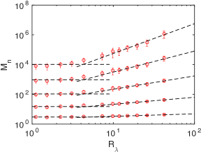
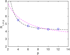
On Fig.1, these ideas have been confirmed by direct numerical simulations (DNS) of the the moments of derivatives $M_{2n}$ vs Reynolds number based on the Taylor scale $R_{\lambda}=\sqrt{\frac{5}{3{\cal E}\nu}}v_{rms}^{2}$. We can see horizontal lines corresponding to the Re-independent normalized Gaussian moments $M_{2n}=(2n-1)!!$ for $2\leq n\leq 6$.

Figure 1: Left panel: Normalized moments of velocity gradients $M_{2n}$ from direct numerical solutions to the Navier-Stokes equations (2)-(3). Both asymptotics, leading to predicted matching relation (4), are clearly seen. Middle panel: Reynolds number dependence of different-order moments $M_{2n}(Re)$. From Ref. [3]-[4]. Right panel: theoretical construction leading to the second-order moment $e_{2}\propto\overline{{\cal E}^{2}}$ in the entire range of $Re$-variation. The low-Reynolds input : $Re_{2}^{tr}\approx 100-120$ and $e_{2}=3.0$ for $Re<100$. This gives $d_{2}\approx 0.157-0.167$. In the strong coupling range $e_{2}=1.45\times Re^{0.157}$.

We would like to stress an important point: $v_{rms}$ characterizes typical or relatively mild velocity fluctuations. In general, to be able to predict rare, extreme, events we introduce $\hat{v}_{2n}=L^{2}\overline{(\partial_{x}v_{x})^{2n}}^{\frac{1}{n}}\propto A_{2n}^{\frac{1}{n}}Re^{\frac{\rho_{2n}}{n}}$ and $\hat{R}_{\lambda,n}^{tr}=\sqrt{\frac{5}{{3\cal E}\nu}}\hat{v}_{2n}\approx 8.91$ derived in Refs.[3]-[8]. To calculate large- scale transitional Reynolds number we introduce velocity scale $v_{0}=v_{rms}$ so that $Re=v_{0}L/\nu$ and :

$$\hat{R}_{\lambda,n}^{tr}=\sqrt{\frac{5}{3{\cal E}\nu}}\hat{v}_{2n}=A_{2n}^{\frac{1}{n}}(Re^{tr})^{\frac{\rho_{2n}}{n}+\frac{1}{2}}\approx 8.91$$

It follows from this relation that transition to strong turbulence in different realizations or different-order-moments occurs at a constant $R^{tr}_{\lambda,n}=8.91$ but at different $Re^{tr}=v_{rms}L/\nu$ based on the r.m.s. velocity coming from the second-order moment. This result, theoretically evaluated in [5]-[8], is consistent with the empirical ${\cal K}-{\cal E}$ model giving the large-scale “dressed” viscosity $\nu_{T}=0.0845{\cal K}^{2}/{\cal E}$, used in engineering simulations during last fifty years [9]. Indeed: with ${\cal K}=v_{rms}^{2}/2$

$$R^{tr}_{\lambda}\equiv R^{tr}_{\lambda,2}=\sqrt{\frac{5}{3{\cal E}\nu_{T}}}2{\cal K}\approx 8.88$$

and

$$Re_{n}^{tr}=[\frac{\hat{R}_{\lambda,n}^{tr}}{A_{2n}^{\frac{1}{n}}}]^{\frac{2\rho_{2n}}{2\rho_{2n}+n}}$$

The somewhat “unexpected” but qualitatively reasonable consequence of this result, is seen on Fig.1, where the onsets of anomalous scaling for different moments $M_{n}$ are observed at very different $Re_{n}^{tr}$ but at a single $n$-independent $\hat{R}_{\lambda,n}^{tr}\approx 9.0-10$. For large enough $n$, $A_{2n}^{\frac{1}{n}}$ is a weakly dependent function of $n$ which can be calculated from the $Re_{2}^{tr}\approx 9-10$. Thus, one can easily express $Re_{n}^{tr}$ in terms of $\hat{R}_{\lambda,n}^{tr}\approx 9.0-10$ [3] - [4] and close the equation (4) for $\rho_{2n}$. The results are presented in Table II and compared with the data on the middle panel of Fig.1.

I.2 Matching condition: numerical procedure for high-Reynolds number limit.

In addition to the “classic” problem of anomalous exponents $d_{n}$ and $\rho_{n}$, the study of Refs.[3] -[4] opened up a new question of possible universality of transitional Reynolds number $\hat{R}^{tr}_{\lambda,n}=\sqrt{\frac{5}{3{\cal E}\nu}}\hat{v}_{2n}\approx 8.91$ derived in the Renormalization Group analysis of turbulence in the limit $r\rightarrow L$ [5]-[9]. The possible universality of this result may have important consequences for numerical simulations demonstrated in Fig.1 where the analytic theory is compared to the low Reynolds number DNS on the two left panels. In the Gaussian forcing case [3]-[4]:

$$Re^{tr}_{n}=C(\hat{R}^{tr}_{\lambda,n})^{\frac{n}{d_{n}+\frac{3n}{2}}}$$ (5)

and at transition points the matching condition must be satisfied:

$$e_{n}=\overline{({\cal E}/\overline{\cal E})^{n}}=(2n-1)!!=C^{d_{n}}(\hat{R}^{tr}_{\lambda,n})^{\frac{nd_{n}}{d_{n}+\frac{3n}{2}}}$$ (6)

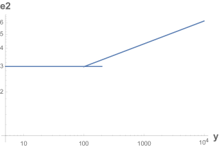
where $\hat{R}_{\lambda,2n}^{tr}\approx 8.91$ independent on $n$. One can easily derive a simple estimate $Re\approx 1.5R_{\lambda,2}^{2}$ giving $Re_{2}^{tr}\approx 100-200$ resulting in $C\approx 100-200$. This closes the equation for exponents $d_{n}$ and $\rho_{2n}$: if, as in the problem $(2)-(3)$, $\overline{\cal E}\approx D_{0}=O(1)$, then $\rho_{2n}=d_{n}+n$. The details are presented in [4]. The possible universality of transitional $R^{tr}_{\lambda,n}$ enables high-Reynolds number computations of flows based on the low-Reynolds number data obtained either theoretically or numerically. The matching procedure is qualitatively demonstrated on the right- most panel of Fig.1 on an example of the moment $e_{2}(y)$ where $y\propto Re_{2}-Re_{2}^{tr}$. It consists of three main steps: a. calculate or compute the moments of derivatives in the linear low-Reynolds number limit $\hat{R}e_{n}\leq\hat{R}e_{n}^{tr}\approx 120$ or $\hat{R}_{\lambda,n}\leq R_{\lambda,n}^{tr}\approx 8.91$. b. This allows evaluation of the exponents $d_{n}$ and $\rho_{n}$. c. Extrapolation of an assumed high-Reynolds number solution $e_{n}=C^{d_{n}}Re^{d_{n}}$ back to the transition point, $Re\rightarrow Re^{tr}_{n}$. c. Plot the resulting dependence in the entire range $Re\geq Re_{n}^{tr}$. Below we generalize this scheme to a much more complex system.

$n$	$1$	$2$	$3$	$4$
$R_{\lambda,2n}^{tr}$	$8.91$	$5.5$	$4.8$	$4.5$
$Re_{2n}^{tr}$	$126$	$45$	$35$	$30$

Table 2: Transitional Reynolds numbers based on Taylor scale $R^{tr}_{\lambda,2n}=\sqrt{\frac{5}{3{\cal E}\nu}}v_{rms}^{2}$ of the moments $M_{2n}$. With $\hat{v}_{2}=\overline{v^{2n}}^{\frac{1}{n}}$, the modified Reynolds number $\hat{R}_{\lambda,2n}^{tr}=8.91$ is independent on $n$.

$\rho_{n}$	$EXP$	$GAU$	$DNS$
$\rho_{1}$	$0.48$	$0.46$	$0.455$
$\rho_{3}$	$1.55$	$1.58$	$1.478$
$\rho_{4}$	$2.12$	$2.19$	$2.05$
$\rho_{5}$	$2.7$	$2.82$	$2.66\pm 0.14$
$\rho_{7}$	$3.92$	$4.13$	$3.99\pm 0.65$

Table 3: Comparison of exponents $\rho_{2n}=d_{n}+n$ with the outcome of numerical simulations (DNS) and Theory. $EXP$ and $GAU$ from expression (14) with the moments $e_{n}=n!$ and $e_{n}=(2n-1)!!$ in flows stirred by exponential and Gaussian random forces, respectively.

II Boundary layer effects.

The simplified problem of Refs. [3]-[4], described above, dealt with an artificial situation of direct transition between a well-defined Gaussian state of a fluid and the non-linearity-dominated strong turbulence. In the case of ”direct transition”, described by (2)-(3), turbulence is produced by a singe physical mechanism, i.e. external random forcing. In real-life flows various randomness - generating mechanisms often act simultaneously: for example in wall flows turbulence is generated by instability of a quasi-laminar flow pattern in the bulk and by instability of viscous wall layers generating powerful bursts reaching bulk of a flow. Therefore, while as $y\propto Re-Re_{cr}\rightarrow 0+$ , the velocity field often obeys Gaussian statistics, at intermediate, but still linear regime, due to the wall boundary layer instability, transition to strong turbulence and anomalous scaling of velocity derivatives may happen not from the Gaussian state. Below we address this problem.

The problem of thermal convection in a fluid heated from below is a remarkable laboratory for studying different areas of physics like heat conduction, pattern formation, their stability and instabilities as well as transitions to chaos and strong turbulence. It is perfectly suited for studies of small-scale structure in a strongly non-linear turbulent state in the limit $Re\rightarrow\infty$. In general, the problem is very hard, for it involves the first instability leading to rolls, generation of the low-Re “weak turbulence” which is a precursor to the strong “hard” turbulence we are interested in this paper. The number of both experimental and theoretical publications dealing with RB convection published in the last few decades is enormous and it is impossible even to briefly review them. Majority of the work in the field dealt with the large-scale global properties of the phenomenon leading to predictions of the heat transfer as a function of various large-scale parameters. Here we are interested in the small-scale velocity and velocity derivatives fluctuations, which is a relatively new and interesting topic.

This problem has been addressed in the DNS published in a recent paper [10] on the RB convection with Prandtl and Reynolds numbers varying in the range $0.005\leq Pr\leq 100$ and $1\leq Re\leq 1000$. At large $Re\approx 100-2000$ the scaling exponents of the first two moments of kinetic energy dissipation rate were similar to those observed in Ref.[4], indicating possible universality. On the other hand, the low-Re behavior of a flow, reflecting some structural transitions, was much more complex and appearance of anomalous scaling at $Re\approx 100$ was definitely not from a Gaussian state of Refs.[3]-[4]. In this case, unlike the direct transition, the Reynolds number dependence of moments of derivatives $M_{2n}(Re)$ was nonmonotonic having a well - pronounced minima in the low-Re interval [10]. While this paper shed light on many important phenomena related to the Prandtl number dependence of the heat transfer, the details of statistics of the dissipation rate fluctuations, including the non-monotonic behavior of the moments, remained somewhat unresolved, mainly due to large difference between thermal and viscous boundary layers substantially complicating the situation.

Below, based on a general approach developed by Sinai et.al. [10]-[12] we consider a greatly simplified problem of thermal convection in a gap $H$ between two infinite plates.

II.1 Phenomenology.

In this paper we are interested in the small-scale behavior of a flow between two infinite plates separated by the gap $H$. The low plate at $z=-H//2$ is heated by an electric current $I$. Due to the energy conservation, the heat flux averaged over horizontal planes $J(z)=cost$ and we keep the top and bottom plates under constant temperature difference $\Delta$. We consider the coupled three-dimensional equations of motion for velocity and temperature fluctuations $v_{i}$ and $T$, respectively:

$$\frac{\partial v_{i}}{\partial t}+v_{j}\frac{\partial v_{i}}{\partial x_{j}} =-\frac{\partial p}{\partial x_{i}}+\nu\frac{\partial^{2}v_{i}}{\partial x_{i}{{}^{2}}}+\alpha gT\delta_{i3}\,,$$ (7)

$$\frac{\partial T}{\partial t}+v_{j}\frac{\partial T}{\partial x_{j}}, =\kappa\frac{\partial^{2}T}{\partial x_{j}^{2}}+\kappa\frac{\partial^{2}\Theta}{\partial x_{j}^{2}}-v_{3}\frac{\partial\Theta}{\partial x_{3}}\,,$$ (8)

Here the horizontally averaged temperature $\Theta=\Theta(z)$ and $\partial_{j}v_{j}=0$. It follows from equation (7) the balance:

$$\overline{{\cal E}}=-\alpha g\overline{v_{3}T}$$

stating that mean kinetic energy production by temperature fluctuations is balanced by the dissipation ratel. Below, this relation will be used for normalization, so that

$$e_{1}=\frac{\overline{{\cal E}}}{-\alpha g\overline{v_{3}T}}=1$$

and we will be interested in evaluation of all moments $e_{n}=\frac{\overline{{\cal E}^{n}}}{(\alpha g)^{n}\overline{(v_{3}T)}^{n}}$.

According to (7), to understand small-scale features of a flow, we have to investigate temperature fluctuations acting as a forcing term in the Navier-tokes equation (7). Below, we use the theory of probability density (PDF) of temperature fluctuations in RB convection developed in the nineties [11]-[12]. In the low-Rayleigh number linear and weakly non-linear regimes, the following results, relevant for this study, have been firmly established [13]-[17].

1.  At $Ra<1708$ the heat transfer is governed by conduction with heat flux $J=\kappa\frac{\partial\Theta}{\partial x_{3}}=\nu\frac{\partial\Theta}{\partial z}=const$ and ${\bf v}=0$;
2.  First, at $Ra\approx Ra_{cr}\approx 1700$, instability of a linear temperature profile with ${\bf v}=0$, typical of conduction, leads to formation of a ”quasi-steady” large-scale flow pattern called rolls.
3.  Then, in the interval $6\times 10^{4}-5\times 10^{6}$, weak fluctuations around this ordered flow field lead to the low - amplitude, $O(Ra-Ra_{cr})\ll Ra_{cr})$, velocity and temperature fluctuations. In this range, according to Krishnamurti [14] and Busse [15], convection consists of ordered rolls with embedded small-scale fluctuations they call “convection elements”. It is important that, while rolls are characterized by the length-scale $r\approx H$, the small-scale elements “live” on the scale $r\ll H$, independent on $H$. Quoting Busse [15]: ‘’At moderate Prandtl numbers, turbulent convection at Rayleigh numbers of the order of $10^{5}-10^{7}$ exhibits the typical structure of relatively steady large-scale cells in which highly fluctuating (both in space and in time) small-scale convection elements are imbedded”. Similar results have been reported in a detailed study of Castaing et.al. [13], showing a few peaks on the heat transfer curves before the rise of “hard” turbulence at $Ra\approx 4\times 10^{7}$. In a relatively recent paper, P. Tong et. al. [17] reported two competing mechanisms of heat transfer originating from the fluctuations in a bulk of convection cell and plumes produced by instabilities of viscous sublayers. The most important lesson from the existing experiments for what follows is emergence of a few qualitatively different contributions to the heat transfer in a soft turbulence range of $Ra$ variation.
To solve (7)-(8), following [10]-[12], the domain of variation of both velocity and temperature fields, can be subdivided in two parts. a.  The wall region with thin ($\eta<<H$) velocity and temperature boundary layers (BL). Due to the no-slip boundary conditions ${\bf v}_{top}={\bf v}_{bot}=0$, strong wall shear leads to the boundary layer instability manifested in discrete bursts in the directions of the bulk. Similar mechanism of turbulence production in channel flows, responsible for the low Reynolds number Blasius scaling of the friction coefficient, was recently discussed in [16]. This leads to generation of velocity/temperature fluctuations in the bulk.
b.  Thus, we will study convection outside boundary layers, using the phenomenology of the BL physics as an approximate boundary conditions for equations defined in the bulk. In this domain turbulence can be assumed isotropic and homogeneous.
4.  In the high Reynolds number limit $Ra\gg Ra_{cr}$, the flow becomes strongly non-linear and the notion of well-separated plumes invalid: due to strong interaction they loose their individuality in the bulk of the cell. This limit is characterized by strong small-scale intermittency and anomalous scaling.

III Statistical ensemble. Probability Density $P(X)$. Low ”Reynolds Number”.

Here we consider an infinite fluid between two horizontal plates separated by a gap $H$. The integral scale of turbulence is $L\geq H$ and thus, the flow is generated in a huge number $N\approx{\cal L}/H\rightarrow\infty$ of independent statistical realizations. Therefore, one can use the theory of a passive scalar proposed by Sinai and Yakhot [11] and applied to the problem of Benard convection in Ref.[12].
Since in the field of large-scale rolls, $\frac{\partial v_{3}}{\partial t}\approx V\frac{\partial v_{3}}{\partial z}$, we define the “low - Reynolds number regime” by the range where the non-linearity in (7) can be neglected,

$$V\frac{\partial v_{3}}{\partial z}-\nu\frac{\partial^{2}v_{3}}{\partial x_{p}^{2}}=\alpha gT$$ (9)

plus no-slip boundary conditions on solid walls. With ${\cal E}_{3}=\nu(\frac{\partial v_{3}}{\partial x_{p}})^{2}$:

$$\frac{{\cal E}_{3}}{\overline{{\cal E}_{3}}}+\frac{\frac{V}{2}\frac{\partial v_{3}^{2}}{\partial z}-\frac{\nu}{2}\frac{\partial^{2}}{\partial x^{2}_{p}}v_{3}^{2}}{\overline{\cal E}_{3}}=\frac{v_{3}T}{\overline{v_{3}T}}$$

From the heat equation we have:

$$\frac{(\nabla T)^{2}}{\overline{(\nabla T)^{2})}}=\frac{v_{3}T}{\overline{v_{3}T}}$$

Defining $\hat{\cal E}=\nu(\frac{\partial v_{3}}{\partial z})^{2}$, gives:

$$\hat{\cal E}-\frac{2\nu^{2}}{V}\frac{\partial v_{3}}{\partial z}\frac{\partial^{2}v_{3}}{\partial x_{p}^{2}}+\frac{\nu^{3}}{V^{2}}(\frac{\partial^{2}v_{3}}{\partial x_{p}^{2}})^{2}=\nu(\frac{g\alpha}{V})^{2}T^{2}$$

Based on the theory [11]-[12] supported by experimental data [13]-[[15], [17], ]we conclude that there exist two mechanisms of dissipation of kinetic energy ${\cal E}_{3,1}\propto T^{2}$ and ${\cal E}_{3,2}\approx b|T|$, with continuous $O(T^{2})$ contribution coming from the “convection elements” and the $O(T)$ one from the discrete plumes arising from the BL instability at $Ra\geq 1700\eta^{bl}/H$ with the typical rising velocity $V$. Obtaining this estimate we relied on the concept “marginally stable” boundary layer introduced by Malkus [18] and discussed Castaing et.al [13].

We are interested in probability density $P(X)$ in the limit of small $X=T/T_{rms}$. This range includes heat conduction regime, formation of weakly fluctuating rolls and discrete plumes coming boundary layers. As in Refs. [10] -[12], it is assumed that in the central part of the cell the fluid is well mixed and turbulence there can be assumed homogeneous and isotropic. Following [11], [12] multiplying (8) by $T^{2n-1}$ gives:

$$-(2n-1)\overline{T^{2n-2}(\nabla T)^{2}}=\overline{T^{2n-1}v_{3}}\frac{\partial\Theta}{\partial z}$$

With $X^{2}=T^{2}/\overline{T^{2}}$, $Y^{2}=(\nabla T)^{2}/\overline{(\nabla T)^{2}}$ and $W=v_{3}T/\overline{v_{3}T}$. These equations can be rewritten:

$$(2n-1)\overline{X^{2n-2}Y^{2}}=\overline{X^{2n-2}W}$$

and introducing conditional means gives [10]-[12]:

$$(2n-1)\int X^{2n-2}r_{1}(X)P(X)dX=\int X^{2n-2}r_{3}(X)P(X)dX$$

where

$$r_{1}(X)=\frac{\int Y^{2}(x)\delta(X(x)-X)dx}{\int\delta(X(x)-X)dx}$$

and

$$r_{3}(X)=\frac{X}{\overline{v_{3}X}}\frac{\int v_{3}(x)\delta(X(x)-X)dx}{\int\delta(X(x)-X)dx}$$

$r_{1}(X)$ and $r_{3}(X)$ are conditional expectation values of temperature dissipation and production rates for fixed magnitude of dimensional temperature $X$. After simple manipulations one obtains a formal expression for probability density $P(X)$ [10]-[12]:

$$P(X)=\frac{C}{r_{1}(X)}\exp\big{[}-\int_{0}^{X}\frac{r_{3}(u)du}{ur_{1}(u)}\big{]}$$

or

$$P(X)=\frac{C}{r_{1}(X)}\exp\big{[}-\int_{0}^{X}\frac{uv_{3}(u)du}{ur_{1}(u)}\big{]}$$ (10)

We can evaluate this expression in the limit $X\rightarrow 0$. First, according to [11]-[12], positive definite conditional dissipation rate

$$r_{1}(X)\approx\alpha+\beta X^{2}=\alpha(1+\frac{\beta}{\alpha}X^{2})$$

Since positive temperature fluctuations (blobs of hotter fluid) are carried by positive velocity fluctuations $v_{3}$, we conclude that $v_{3}(T)\approx-v_{3}(-T)$.

As $Ra-Ra_{cr}\rightarrow 0$, the fluctuations of the large-scale rolls, called “convection elements” are very weak, lacking any typical velocity scale. Therefore, in this limit by the symmetry: $v_{3}(X)\propto X$. At larger Rayleigh number the instability of viscous sublayers leads to plumes emitted with a typical velocity $V=yV_{p}$ where we introduce an artificial Reynolds number $y\propto Re-Re(p)$ with $Re(p)$ denoting the Reynolds number of first instability of boundary layer (manifested in peaks in a heat flux curve) resulting in weak discrete bursts. This means that in this theory $y\geq 0$ and the conditionally averaged velocity can be written as:

$$\frac{v_{3}(X)}{v_{rms}}\approx\gamma X+2yV_{p}/v_{rms}\approx\gamma X+2\kappa y$$

where $V_{p}/v_{rms}=O(1)$. We can see that when $y=0$, the resulting Gaussian flow is dominated by the weak small-scale elements. Substituting all this into (10) gives:

$$P(X,y)=\frac{C(y)}{(1+\frac{\beta}{\alpha}X^{2})}\exp[\big{[}-\int_{0}^{X}\frac{\gamma u+2\kappa y}{\alpha(1+\frac{\beta}{\alpha}u^{2})}du\big{]}$$

and the probability density of temperature fluctuations in the central part of convection cell with $\alpha=\kappa=1$ is:

$$P(X,y)=\frac{C(y)}{(1+\frac{\beta}{\gamma}X^{2})^{1+\frac{\gamma}{2\beta}}}exp(-2y\arctan(\sqrt{\beta}X)\equiv$$

$$C(y)\Pi(X,y)$$ (11)

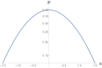
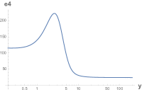
with $C(y)=1/2\int_{0}^{\infty}\Pi(X,y)dX$ and $\beta\approx 1.4$ estimated in [12]. As $y\rightarrow 0$, this expression gives Gaussian with the half-width $\delta\approx\sqrt{\gamma/\beta}$. It has been found in Ref.[12] that although the derivation is, strictly speaking, valid for $\frac{\beta}{\gamma}X^{2}\rightarrow 0$, the result agrees very well with numerical simulations in a much broader interval. An interesting feature of this expression is the dependence of the PDF on Reynolds number $y$. This is the consequence of a qualitative transition happening in the flow $y>0$. The behavior of the PDF as a function of “Reynolds number” $y$ is shown on Fig.1.

III.1 Moments of dissipation rate. Low-Re regime.

Based on the above derivation (also see Ref.[12]), the conditional mean of kinetic energy dissipation rate is approximated by the expression:

$$\frac{\cal{E}}{\overline{\cal E}}\approx yX+X^{2}$$ (12)

and thus, the normalized moments of the dissipation rate are calculated readily

$$e_{n}(y)=\frac{\int_{0}^{\infty}(yX+X^{2})^{2n})P(X,y)dX}{(\int_{0}^{\infty}(yX+X^{2})^{2})P(X,y)dX)^{n}}$$

Figure 2: Probability densities of normalized dissipation rate $e={\cal E}/\overline{\cal E}$ vs ”Reynolds number” $y$.
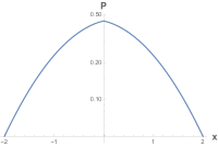
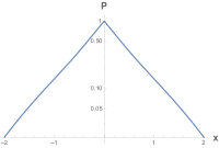
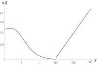
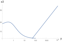
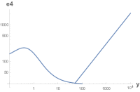
Top panel: $y=0.01$. Middle: $y=0.1$. Bottom: $y=1.$. In all cases $\beta=1.4$ as estimated in [12]-[13].

Figure 3: Nonmonotonic low- Reynolds number behavior of normalized moments of kinetic energy dissipation rate $e_{n}=\frac{\overline{{\cal E}^{n}}}{\overline{\cal E}^{n}}$ as a function of artificial ” Reynolds number” $y\propto Re-Re(p)$ , first observed in Ref.[10]. At $y\rightarrow 0$, all $e_{n}(y)\approx(2n-1)!!$ indicating Gaussian statistics. With increase of $y$, one can see transition to a state dominated by weak structures and close-to-exponential probability densities. The range $Re>>Re_{n}^{tr}$ corresponds to strong coupling where the quasi-linear approximation breaks down.

Figure 4: Analytic procedure for evaluation of moments of dissipation rate in the entire Reynolds number range $0\leq y\leq\infty$. Given the low-Reynolds number moments $e_{n}(y)$ (Fig.3) and transitional Reynolds numbers $Re_{2}^{tr}\approx 100$, the exponents $d_{n}(y)$ and $\rho_{2n}(y)=d_{n}(y)+n$ for the moments $e_{n}(y)$ and $M_{2n}(y)$, vali in strongly non-linear, anomalous, regime. $Re_{n}^{tr}\leq Re<\infty$ are calculated from (14). The two limiting curves match at $Re=Re_{n}^{tr}$. On this graph: $Re\rightarrow\infty$, $e_{2}\propto Re^{0.157}$, $e_{3}\propto Re^{0.46}$ and $e_{4}\propto Re^{0.83}$.

Figure 5: Ratio of scaling exponents $\rho_{2n}=d_{n}+n$ in flows driven by exponential and gaussian random forces vs $n$. .

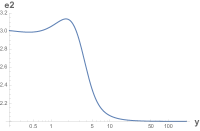
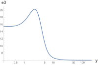
This expression is valid when Reynolds number is so small that the non-linearity in (7) can be neglected, but large enough to allow for the relatively weak boundary layer instability leading to isolated (discrete) plumes. This mechanism is similar to the one considered in [16] responsible to the intermediate Blasius scaling in a channel flow.
In the interval $y\ll X$, $yX<X^{2}$ and the probability density $P(X)$ is close to the Gaussian with the first few low-order moments $e_{n}\propto\overline{X^{2n}}\approx(2n-1)!!$.

It is interesting that the expression (12) with $y\propto Re-Re^{tr}$, reflects two competing mechanisms experimentally observed by Tong et.al. [17]. Indeed, when $y\rightarrow 0$, the scale-lacking-excitations dominate the Gaussian PDF. One can also see, that as the “Reynolds number” $y$ grows, due to appearance of discrete plumes $yX>X^{2}$, the PDF (11) varies to close- to -exponential which is an immediate precursor to anomalous scaling and intermittency. The smooth transition from $e_{n}=(2n-1)!!$ to $e_{n}=n!$, experimentally and numerically observed in Refs.[13] and [10], respectively, is shown on Figs. 2-3.

III.2 Matching condition: Strong turbulence, Intermittency in Benard convection

It follows from the theory developed in [4] (also see Section I) that, to describe strongly non-linear limit of turbulent fluid, $Re\rightarrow\infty$, one has to understand fluid behavior in the weakly non-linear range $0\leq Re\leq R^{tr}_{n}\approx 120$. It is a matching of low and high -Reynolds -number asymptotic solutions gives an equation for the amplitudes and anomalous exponents in the strong turbulence interval $Re_{n}^{tr}\leq Re<\infty$. Direct transition from from “normal” to “anomalous” scaling in the Gaussian-force-driven fluid, described in Ref.[3]-[4], [10] and in Section II of this paper, is relatively simple: the derivative moments are equal to $M_{2n}=(2n-1)!!$ in the low-Re range $0\leq Re_{n}^{tr}\approx 100-120$ or $R^{tr}_{\lambda,n}\approx 8.91$.

If at $Re\ll Re_{n}^{tr}$ the moments are $e_{n}=(2n-1)!!$ or $e_{n}=n!$ as in Gaussian or exponential cases, respectively, one has to understand relations between these states as a function of Reynolds number. It is promising that the low-Re range behavior of a flow can be addressed numerically using direct numerical simulations. In a general case of the Reynolds number dependent moments, the exponents $d_{n}(y)$ are found from the equation:

$$e_{n}(y)=\overline{({\cal E}/\overline{\cal E})^{n}}=C^{d_{n}(y)}(\hat{R}^{tr}_{\lambda,n})^{\frac{nd_{n}(y)}{d_{n}(y)+\frac{3n}{2}}}$$ (13)

where $e_{n}(y)$ are found from Fig.3. The result is.

$$d_{n}(y)=-\frac{1}{2}[n(\frac{2.19}{\ln C}+\frac{3}{2})-\frac{\ln e_{2n}}{\ln C}]+$$

$$\sqrt{\frac{1}{4}[n(\frac{2.19}{\ln C}+\frac{3}{2})-\frac{\ln e_{2n}}{\ln C}]^{2}+\frac{3}{2}n\frac{\ln e_{2n}}{\ln C}}$$ (14)

IV Summary and discussion. Universality.

The direct transition from a Gaussian flow ( $R_{\lambda}^{tr}\leq 8.91$), was investigated both theoretically and numerically in Ref[.3]-[4]. The results, based on transitional Reynolds number $R_{\lambda,2}^{tr}=8.91$, and the amplitude $C\approx 90-100$, are presented on Fig.1. It is clear from Fig.2 that in the case of RB convection the low-Re dynamics are much more involved and in the limit $y\propto Re-Re_{cr}\rightarrow 0$, the flow is indeed close-to-Gaussian and can be treated using the results of Sec.I. However, to obtain the moments at a transitional Reynolds number, precursor to anomalous scaling, one has to understand fluid dynamics at the moderate Reynolds numbers $Re\leq Re_{n}^{tr}\approx 100$ or $R_{\lambda}\approx 8.91$. The main question is: how universal this number is?

The universality of the Reynolds number based on “turbulent” viscosity $R_{\lambda,T}\approx 10.0$, derived from dynamic Renormalization Group [5]-[8], widely used in engineering [9], is known for many years. In fact, it is the basis of the so-called ${\cal K}-{\cal E}$ modeling (see Section I) and Ref.[9]. Numerical and experimental data on flows past the cylinder, decaying turbulence and even flow past various industrial applications like cars, gave for the Reynolds number based on “turbulent viscosity” $R_{\lambda}^{T}\approx 9.0-11.0$. In Ref.[5] the transition to anomalous scaling $R_{\lambda}^{tr}\approx 9.0$ has been first reported in the DNS of the Navier- Stokes equations on a periodic domain driven by a force ${\bf f}\approx\alpha{\bf v}$ defined at the large scales with $\frac{2\pi}{L}=k\approx 1-2$, completely different from the one discussed in Refs.[3]-[4]. Possible universality of this number may be not too startling. Indeed, while in open, far from equilibrium, system the “bare” $Re_{cr}$ of the first instability of a laminar pattern may vary in a broad interval, the “dressed” one, characterizing transition from “normal” to anomalous dimensions (intermittency) can be fixed at $R^{tr}_{\lambda}\approx 10$. The possible universality of transitional $R_{\lambda,tr}\approx 9.0$ may have interesting implications. Anomalous scaling is usually related to coherent structures appearing in a coherence-lacking background random flow. If this is so, then it is not impossible that universality of $R^{tr}_{\lambda}$ may indicate universal, flow-independent, structures responsible for transition to strong turbulence. In the future publication The variation of flow geometry at $R^{tr}_{\lambda}\geq 9.0$ has recently been reported by Das and Girimaji [19] in homogeneous and isotropic turbulence driven by a random force. How universal the effect is remains an open and interesting question. We expect the ”magic number” $R_{\lambda}^{tr}\approx 8.91$ to be related to Feigenbaum numbers describing transition in terms of period-doubling mechanism.

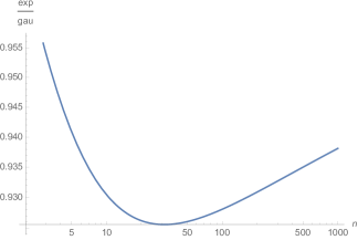
To study the role of the forcing statistics we, assuming for the sake of argument, universality of constants $R_{\lambda,2}^{tr}\approx 9.0$, and $C\approx 90-100$, evaluated the exponents $d_{n}$ from the expression (14). The ratio of exponents $\rho_{2n}=d_{n}+n$ in the flows driven by gaussian and exponential forces, respectively, is plotted on Fig.5, for $y=4.5$ , in the huge, not experimentally realizable interval $2\leq n\leq 1000$. One can see the ratio varying in the range $0.925\leq\frac{exp}{gau}\leq 0.955$, which, though quite close to unity, may indicate existence of universality classes reflecting mechanisms driving turbulence flow.

To conclude the paper we would like to pose a question which can readily be resolved in future numerical and physical experiments: how general is the passage to turbulence, described in this paper, in a typical wall flow where the randomness-generating bulk and wall-layer instabilities often coexist ?

Given the results of Ref.[16], this generality may not be impossible. The role of weak-to-strong turbulence transition in chemical kinetics, combustion and mixing in high-Reynolds number fluids may be of importance in various, at present not explained, processes.

References

- (1) L. D. Landau and E. M. Lifshitz, Course of Theoretical Physics, Statistical Physics, Volume 5, Butterworth-Heinemann, Oxford, 1980.
- (2) A.M. Yaglom, Hydrodynamic Instability and Transition to Turbulence Springer, ,2012.
- (3) V. Yakhot and D. A. Donzis, Phys. Rev. Lett. 119, 044501 (2017).
- (4) V. Yakhot and D. A. Donzis, PhysicaD. xx, 044501 (2018).
- (5) J. Schumacher, K. R. Sreenivasan, and V. Yakhot, New J. Phys. 9, 89 (2007).
- (6) V. Yakhot and L. Smith, “The renormalization group, the -expansion and derivation of turbulence models”, J. Sci. Comp. 7, 35 (1992).
- (7) V. Yakhot, “Reynolds number of transition and self-organized criticality of strong turbulence”, Phys. Rev. E,90, 043019 (2014).
- (8) V. Yakhot, S.A. Orszag, T. Gatski, S. Thangam and C. Speciale, “Development of turbulence models for shear flows by a double expansion technique”, Phys. Fluids A4, 1510 (1992);
- (9) B.E. Launder and D.B. Spalding, “Mathematical Models of Turbulence”, Academic Press, New York (1972); In turbulence modeling literature model is used with experimentally determined coefficient instead of the derived .
- (10) J. Schumacher, A.Pandey, V.Yakhot, and K.R.Sreenivasan, Transition to turbulence scaling in Rayleigh-Benard convection Phys.Rev.E, 98, 033120 (2018)
- (11) Ya.G. Sinai, and V. Yakhot, Phys. Rev. Lett. 63, 1965 (1989). V. Yakhot, Phys. Rev. Lett. 63, 1965 (1989).
- (12) V. Yakhot, S. A. Orszag, S. Balachandar, E. Jackson, Z.-S. She, and L. Sirovich, J. Sci. Comput. 5 (3), 199 (1990).
- (13) B. Castaing, G. Gunaratne, F. Heslot, L. P. Kadanoff, A. Libchaber, S. Thomae, X.-Z. Wu, S. Zaleski, G. Zanetti, J. Fluid Mech. 204, 1 (1989).
- (14) R. Krishnamurti, J . Fluid Mech. 33 457-631970a; J. Fluid Mech. 42 295-307 1970b;
- (15) Busse, F. H., Non-linear properties of thermal convection 1978 Rep. Prog. Phys. 41 1929
- (16) V.Yakhot, S.Bayley, A.J.Smits, Scaling of global properties of turbulence and skin friction In pipe and channel flows. J.Fluid Mech.652,65 (2010)
- (17) X.He and P.Tong, Measurements of thermal dissipation field in Benard convection Phys.Rev.E,79,026306 (2009)
- (18) W. V. R. Malkus, Proc. R. Soc. Lond. A 225, 185 (1954).
- (19) R.Das and S.Girimaji, On the Reynolds number dependence of velocity structure and dynamics, J.Fluid.Mech. 2018 (in press)).
- (20) M. Shifman, QCD Sum Rules: Bridging the Gap between Short and Large Distances. arXiv:1101.1122v1 [hep-ph], 2011