A new multilayer optical film optimal method based on deep q-learning

Abstract

Multi-layer optical film has been found to afford important applications in optical communication, optical absorbers, optical filters, etc. Different algorithms of multi-layer optical film design has been developed, as simplex method, colony algorithm, genetic algorithm. These algorithms rapidly promote the design and manufacture of multi-layer films. However, traditional numerical algorithms often converge to local optimum. This means that these algorithms can not give a global optimal solution to the material researchers. In recent years, due to the rapid development of artificial intelligence, to optimize optical film structure using AI algorithm has become possible. In this paper, we will introduce a new optical film design algorithm based on the deep Q learning. This model can converge the global optimum of the optical thin film structure, this will greatly improve the design efficiency of multi-layer films.

1 Introduction

After the 1970s, with the development and application of computer technology and various numerical optimization techniques. Many traditional numerical optimization algorithms, such as linear programming, simplex method, least square method, damped least squares method were applied to the design of optical thin film. In which the least square method was the most successful application. The shortages of this several method are, this methods are focus on find the local optimum value of the film coating. The optical film researchers also developed a variety of global optimal methods that can be optimized in the film structure. Tikhonravov, Alexander V., and Michael K developed a optical coating design software system based on needle optimization technique. [1] Sullivan, Brian T., and J. A. Dobrowolski. implemented the needle optimization method, and improve design system performance, The improved needle algorithm can not only define very complex evaluation functions but also can be used in many forms to calculate and design, It made the design of optical thin film becomes more flexible.[2] C.P. Chang and H.Y. Lee apply the GSAM(generalized simulated-annealing method) thin-film system design and find that there is no local minimal trapping problem in 1990.[3]. Martin, S applied genetic algorithms to the design of three very different optical filters.[4] In recent decade, this field researcher develop the optical coating optimization system based on several model as, GA, ant colony algorithm, particle swarm optimization and so on.[5][6][7]

In past several years, machine learning was widely used in many research field, as computer vision, automatic robot, medical, finance, etc. It make a big change for our society. [8] Thanks to the growth of computing power, many deep learning methods have been developed by scientists and researchers to solve problems in various fields. The deep reinforcement learning(DRL) is a successful method, which refers to goal-oriented algorithms. It means DRL could learn how to attain a complex objective (goal) or maximize along a particular dimension over many steps.[9] The famous application of DRL is Alpha-Go.[10] This research use a deep q network, one kind of a deep reinforcement learning method, to optimal the optical coating. We optimal 2 different optical coating(anti-reflection film and solar selective absorption film) use our proposed method to measure the effectiveness of this method in this paper.

2 Deep Q learning

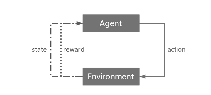
Deep Q learning combines reinforcement learning with a class of artificial neural network known as deep neural networks. There are two basic elements of reinforcement learning: Agent and Environment. Agents act to influence the environment, and then the environment return a feedback to the agent. According this feedback the to decide the next action. Fig.1 is a schematic diagram of the process of reinforcement learning

Figure 1: Reinforcement Learning process

2.1 Markov decision process

It is called Deep Q learning, because the author used a deep neural network to replace a Q-table. Q-table the kernel method in Q learning[11]. In short, deep Q learning develops control patterns by providing feedback on a model’s selected actions, which makes the model to select better actions in the next step.

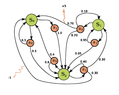
Q-learning is a solution to a Markov decision process. A Markov decision process is defined by an agent, performing in an environment by means of actions, as showed in Fig.2. The environment can be in different states. Markov decision process is a 4-tuple $(S,A,P_{\alpha},R_{\alpha})$. $S$ is a finite set of states, $A$ is a finite set of actions, $P_{\alpha}$ is a transition probabilities, that action $\alpha$ i state $s$ at time $t$ change to state $s_{{}^{\prime}}$ at time $t+1$. $R$ is the reward received, when state $s$ transfer to state $s_{{}^{\prime}}$ under the influence of action $\alpha$.[12][13]

Figure 2: Example of a simple MDP with three states(green circles) and two actions(orange circles), with two rewards(orange arrows)

The set of states and actions, together with rules for transitioning from one state to another and for getting rewards, make up a Markov decision process. One episode of this process forms a finite sequence of states, actions and rewards:

$$s_{0},a_{0},r_{1},s_{1},a_{1},r_{2},s_{2},…,s_{n-1},a_{n-1},r_{n},s_{n}$$ (1)

Here $s_{i}$ is the state, $a_{i}$ is the action and $r_{i+1}$ is the reward after performing the action. The episode ends with terminal state $s_{n}$

2.2 Discounted Future Reward

Considering the long-term situation, not only immediate reward need to be token into account, but also the future awards should be considered. The total reward for one episode in a Markov decision process could be easily calculate as:

$$R=r_{1}+r_{2}+r_{3}+…+r_{n}$$ (2)

The total future reward from time $t$ could be expressed as:

$$R_{t}=r_{t}+r_{t+1}+r_{t+2}+…+r_{n}$$ (3)

Because our environment is stochastic, if every step of action will make a same reward. For long-term situation, it may diverge. For that reason it is common to use discounted future reward instead:

$$R_{t}=r_{t}+\gamma(r_{t+1}+\gamma(r_{t+2}+…))=r_{t}+\gamma R_{t+1}$$ (4)

Here $\gamma$ is the discount factor between 0 and 1. The more into the future the reward is, the less we take it into consideration. It is easy to see, that discounted future reward at time step t can be expressed in terms of the same thing at time step $t+1$.

2.3 Q-learning

Q learning is a model, which approximates the maximum expected return for performing an action at a given state using an action-value Q function. It represents the discounted future reward when we perform action $a$ in state $s$.The Q function is defined as,

$$Q(s,\alpha)=r+\gamma max(Q(s^{{}^{\prime}},\alpha^{{}^{\prime}}))$$ (5)

where $r$ is the reward that was providing feedback from environment, $s$ is the state, $\alpha$ is the action, $\gamma$ is learning rate, and $Q(s^{{}^{\prime}},\alpha{{}^{\prime}})$ comes from predicting the Q function for the next state using our current model.The main idea in Q-learning is that we can iteratively approximate the Q-function using the Bellman equation. In the simplest case the Q-function is implemented as a table, with states as rows and actions as columns. This talbe is called q-table.

2.4 Deep Q-network

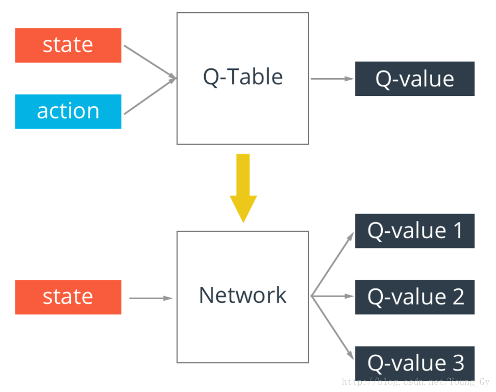
The state of the real situation may be infinite, so that q-table will be infinite. It means the even a supercomputer also can’t calculate the solution of this q-table, when the data or environment is complex. As we know, neural networks are good in optimal highly structured data. We could represent our Q-function with a neural network, that takes the state and action as input and outputs the corresponding Q-value. Fig.3 shows the transformation of Q-learning to deep Q-learning.

Figure 3: Top: The Q-learning model. Bottom: the deep Q-network, used in DeepMind paper.

2.5 Loss functions

In most parts of training process, Q-values can be any real values or any real integer. It determines by the model you want to optimize. So the neural network of deep Q-learning can be optimized with a simple squared error loss.

$$Loss=\frac{1}{2}[r+\gamma max_{a^{\prime}}Q(s^{\prime},a^{\prime})-Q(s,a)]^{2}$$ (6)

$r+\gamma max_{a^{\prime}}Q(s^{\prime},a^{\prime})$ represents the target value. $Q(s,a)$ represents the prediction value.

2.6 Experience reply

Because the we use neural network to approximate the Q-table in Deep Q-learning, so it is not stable in many situation. It will cause the model can not converge or converge to the local optimal value. There are several way to solve this problem. The experience replay is one of the most useful way. When training the neural network, We use random mini-batch from the memory to instead of the recent transition. This breaks the similarity of the training samples, which make our network into a local minimum.

2.7 Exploration exploitation

As the temperature in annealing algorithm, a higher freedom in selecting actions at the beginning is necessary. The model will random select action with probability $\epsilon$.The $\epsilon$ will between 0.1 to 1, and it will decrease with the training process. This technology allows the model to converge faster and avoid convergence in the local optimal.

2.8 Update algorithm

Combining the above methods, the Q-network can be optimized as follow algorithm:

Algorithm 1 Update algorithm of deep Q learning

1:initial the memory $D$

2:initial the $Q$ network with random weights $w$

3:select a random action $a_{t}$ with probability $\epsilon$, otherwise select $a_{t}=argmax_{a}Q(s,a)$

4:Execute action $a_{t}$ in the system environment, observe reward $r_{t+1}$ and new state $s_{t+1}$

5:Store transition $<s_{t},a_{t},r_{t+1},s_{t+1}>$ in memory $D$

6:Sample random mini-batch from $D:<s_{j},a_{j},r_{j},s_{j}^{{}^{\prime}}>$

7:Set $Q_{j}=r_{j}+\gamma max_{a}Q(s_{j}^{{}^{\prime}},a{j}^{{}^{\prime}})$

8:Gradient descent step with a simple squared error loss.

9:for episode = 1, $M$ do

10:     for $T,t$ do

11:     end for

12:end for

3 Application to the Multi-layer Systems

To apply deep Q-network on multi-layer film optimize, we define the state, action, and reward of multi-layer system.

3.1 States

There are several different layer in one multi-layer optical film, each layer have different thickness and different thickness. We define the layer thickness of multi-layer optical film as a state in the optimal system, as:

$$s=Th_{1},Th_{2},..,Th_{n}$$ (7)

For example, in a 4 layer solar absorber film, which structure is $SiO2(90nm)/Cr(10nm)/SiO2(80\\ nm)/Al(\geq 200nm)$.We will define the state as an array[90,10,80] . This array value is according the thickness of each layer.The $Al$ layer is a layer which keep transmission equal to zero in solar absorber film. To reduce the calculation, the $Al$ layer will be ignored.

3.2 Actions

Inspiration from the needle algorithm, the actions defined as increasing or reducing the thickness of one layer in the film coating. The minimum thickness change is determined by the design precision of the film coating. For example, in a $n$ layers film coating with a design accuracy of 0.01 nm, the action will be defined as:

$$A=\{a_{1},a_{2},..,a_{n}\}$$ (8)

$a_{n}$ represents the action on each layers. In this situation $a_{n}$ contains 6 values, each value is an action on the layer $n$ in this film coating.

$$a_{n}=\{x|\pm x=10^{-K},0\geq K\geq N,K\in Z^{+}\}$$ (9)

$N$ represents the precision level of this film coating. In this case,the $N$ is equal $3$, that $a_{n}$ will equal ${\pm 1,\pm 0.1,\pm 0.01}$. We choose several different thickness change is aim to speed up the convergence speed while guaranteeing the accuracy. It’s very easy to understand, an action $a_{n}=1$ will save a hundredfold of the time compared with $a_{n}=0.01$

3.3 Reward

Before define the reward, the aim function of film coating optimal should be defined at first. There are three parameters, transmission $T$, reflection $R$, absorption $A$, are focused in the design of optical film coating design. The reward in our film coating optimal system is defined as 3 value, as:

$$Aim=w_{T}T+w_{R}R+w_{A}A$$ (10)

$w_{T},w_{R},w_{A}$ represent the weights of three parameters. This three weights determined by type of optical thin film. For example, the weights will defined as $w_{T}=0,w_{R}=-1,w_{A}=1$ during designing the solar selective absorber. Because influence of transmission can be ignored, and film need higher absorption and smaller reflection.

$$r_{t}=\begin{cases}0,\text{not find a better value in past 50 steps}\\ -1,\text{aim optical parameters is lower threshold value}\\ Aim_{best}-Aim_{t},{othersituation}\end{cases}$$ (11)

We define a stop search mechanism, when the system not search a better result in several steps. It has the chance to reduce the convergence probability of the model, but it can get the best value after all. Compared with other application of deep Q-learning, our system pays more attention to finding the best solution.

3.4 Neural network structure

Considering the number of actions, we use a two layers full connect neural network in our deep Q-network. Each layer has 80 units.We will random initialize this network. The learning rate will fade with the training of the network.

4 Experiments

In this part, we will show the application performance in 2 different optical coatings(solar selective absorber and high reflection film).

4.1 Solar selective absorber

First we apply deep Q-learning model on $300nm$-$1500nm$ solar selective absorber. 4-layers, 6-layers film structure is very famous structure in solar selective absorber. The materials of film coating use $Ti$ and $SiO_{2}$. The substructure will use $200nm$ $Cu$. The thickness is initialized with $50nm$ for each layer.

Table 1: Solar selective absrober coating after optimized

layer	material	4-layers	6-layers	8-layers
0	Air	-	-	-
1	$SiO_{2}$	132.4	126.0	63.19
2	$Ti$	13.74	6.46	3.47
3	$SiO_{2}$	77.5	73.37	71.46
4	$Ti$	-	12.98	6.19
5	$SiO_{2}$	-	54.56	65.84
7	Ti	-	-	12.45
8	$SiO_{2}$	-	-	52.4
Sub	$Cu$	200	200	200
Absorption		87.4%	90.15%	91.18%

Figure 4: The optimal result of DQN algorithm.

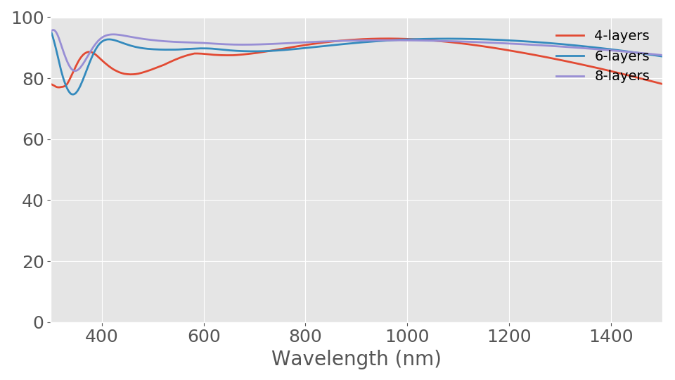
The Table 1 and Fig.4 shows the optimal result of film coating. The initial thickness of each layer could be random. But we do not hope you initialize it very large, it will make you cost many time to get the final good optimal result. In experiments, if the initial film coating is very close to the optimal result it will find the best result very fast. By contrast, it costs much time. But in the end, it will find best optimal result almost irrelevant to the initial value.

4.2 Anti-reflection film

Anti-reflection film is also a very important application in optical film. The anti-reflection film applies on camera lens, solar absorber and so on. In this part, we test a $ZnS$ and $MgF_{2}$ anti-reflection film on $400nm$ to $700nm$. In this experiments, the precision of design is $1nm$. The initial thickness of each layer is $30nm$.So the number of actions is come to equal 18 (9 layers time 2 action of each layer). We compared the result with another optimal technique: GA.

Table 2: Anti-reflection film coating after optimized

layer	material	DQN	GA
0	Air	-
1	$MgF_{2}$	96	90
2	$ZnS$	27	23
3	$MgF_{2}$	14	16
4	$ZnS$	70	71
5	$MgF_{2}$	22	20
7	$ZnS$	24	26
8	$MgF_{2}$	43	40
9	$ZnS$	7	3
Sub	$SiO_{2}$	-	-
Reflection		4.5%	5.9%
transmission		94.0%	92.7%

According the experiments, we could know the Deep Q-learning could find better solution compare with GA in same situation. The spectral curve shows in Fig.5. The reflection distribution of DQN is more uniform.

Figure 5: Left: the optimal result of GA algorithm. Right: the optimal result of DQN algorithm.

5 Conclusion

This paper provides a new method for numerical optimization of optical thin film design. This new method combines machine learning and optical thin film computing. Compared with previous research in the same field, this algorithm has higher search space and better search results. This algorithm can reach the search scope of needle algorithm and the local search precision of GA algorithm.

In our experiments, the initial thickness of the optical thin film could be random. This means that researchers can select materials and perform parallel operations on a large scale according to their requirements. This will greatly improve the efficiency of finding the target film.

6 Acknowledgment

The authors would like to thank Prof.Chen from FuDan Univ. and Prof.Yoshie from Waseda Univ.. These two professors give me a lot of research advice and provided me with a good research environment. The optical film computation part is based on C. Marcus Chuang’s open source project [14]. MorvanZhou give us a great hello wolrd demo of deep Q-learning[15]. The optical constant data is search from refractive index.info this website built by Mikhail Polyanskiy[16]. In the end, I want to thank all those who have given me help in the study of life.

References

- [1] A. V. Tikhonravov and M. K. Trubetskov, “Development of the needle optimization technique and new features of optilayer design software,” in Optical Interference Coatings, vol. 2253 (International Society for Optics and Photonics, 1994), pp. 10–21.
- [2] B. T. Sullivan and J. Dobrowolski, “Implementation of a numerical needle method for thin-film design,” \JournalTitleApplied optics 35, 5484–5492 (1996).
- [3] C. Chang, Y. Lee, and S. Wu, “Optimization of a thin-film multilayer design by use of the generalized simulated-annealing method,” \JournalTitleOptics letters 15, 595–597 (1990).
- [4] S. Martin, J. Rivory, and M. Schoenauer, “Synthesis of optical multilayer systems using genetic algorithms,” \JournalTitleApplied Optics 34, 2247–2254 (1995).
- [5] W. Paszkowicz, “Genetic algorithms, a nature-inspired tool: a survey of applications in materials science and related fields: part ii,” \JournalTitleMaterials and Manufacturing Processes 28, 708–725 (2013).
- [6] J.-j. TANG and S.-j. JIANG, “Coating optimization design based on elite genetic algorithm with adaptive mutations [j],” \JournalTitleOptical Instruments 4, 008 (2006).
- [7] X. Guo, H. Zhou, S. Guo, X. Luan, W. Cui, Y. Ma, and L. Shi, “Design of broadband omnidirectional antireflection coatings using ant colony algorithm,” \JournalTitleOptics express 22, A1137–A1144 (2014).
- [8] R. S. Michalski, J. G. Carbonell, and T. M. Mitchell, Machine learning: An artificial intelligence approach (Springer Science & Business Media, 2013).
- [9] V. Mnih, K. Kavukcuoglu, D. Silver, A. A. Rusu, J. Veness, M. G. Bellemare, A. Graves, M. Riedmiller, A. K. Fidjeland, G. Ostrovski, P. Stig, B. Charles, S. Amir, A. Ioannis, K. Helen, K. Dharshan, W. Daan, L. Shane, and H. Demis, “Human-level control through deep reinforcement learning,” \JournalTitleNature 518, 529 (2015).
- [10] D. Silver, J. Schrittwieser, K. Simonyan, I. Antonoglou, A. Huang, A. Guez, T. Hubert, L. Baker, M. Lai, and A. Bolton, “Mastering the game of go without human knowledge,” \JournalTitleNature 550, 354–359 (2017).
- [11] C. J. C. H. Watkins, “Learning with delayed rewards,” \JournalTitlePh.d.thesis Cambridge University 15, 233–235 (1989).
- [12] R. Bellman, “A markovian decision process,” \JournalTitleIndiana University Mathematics Journal 6, 15 (1957).
- [13] E. Altman, “Constrained markov decision processes,” \JournalTitleChapman and Hall/crc Boca Raton FI 32, 1–22 (1995).
- [14] C. M. Chuang’, “Optical modeling,” [retrieved December 5, 2017]. https://github.com/marcus-cmc/.
- [15] M. Polyanskiy, “Reforcement learning with tensorflow,” [retrieved October 15, 2016]. https://github.com/MorvanZhou/Reinforcement-learning-with-tensorflow.
- [16] M. Polyanskiy, “refractiveindex.info,” [retrieved October 24, 2017]. https://refractiveindex.info/.