Neural Image Decompression:
Learning to Render Better Image Previews
Abstract
A rapidly increasing portion of Internet traffic is dominated by requests from mobile devices with limited- and metered-bandwidth constraints. To satisfy these requests, it has become standard practice for websites to transmit small and extremely compressed image previews as part of the initial page-load process. Recent work, based on an adaptive triangulation of the target image, has shown the ability to generate thumbnails of full images at extreme compression rates: 200 bytes or less with impressive gains (in terms of PSNR and SSIM) over both JPEG and WebP standards. However, qualitative assessments and preservation of semantic content can be less favorable. We present a novel method to significantly improve the reconstruction quality of the original image with no changes to the encoded information. Our neural-based decoding not only achieves higher PSNR and SSIM scores than the original methods, but also yields a substantial increase in semantic-level content preservation. In addition, by keeping the same encoding stream, our solution is completely inter-operable with the original decoder. The end result is suitable for a range of small-device deployments, as it involves only a single forward-pass through a small, scalable network.
1 Introduction
Compression of high-quality thumbnails is an active area of research [36, 33, 1, 18, 3] as the demand for image content over connections of all speeds continues to quickly rise. In addition to the decreased download latency and bandwidth consumption that is particularly important to the “next billion users” (NBU), reducing the compressed-image size also helps with storage requirements for the billions of thumbnails needed for rapid access [13, 6, 16].
Two standard measures of compression quality are PSNR and SSIM [35]. However, at such high-compression rates (200 bytes per thumbnail image, which is 0.033 bpp for thumbnails), we have found that these metrics do not adequately reflect subjective preferences. Therefore, in addition to using PSNR and SSIM, we measure how well semantic information, in terms of recognizable objects and scenes, is preserved.
Similarly, at these extreme-compression rates, JPEG and other standard approaches do not fare well. Usually, when extreme compression is required, it is addressed with domain-specific techniques: for example, faces [5], satellite imagery [15], smooth synthetic images [25], or surveillance [39]. For non-specialized image-compression, WebP [13] is a leading compression format. When used on small images, WebP yields better compression than both JPEG and JPEG2000 standards [12, 14].
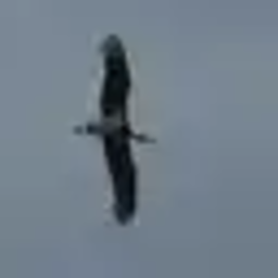
The fundamental operation of both WebP and JPEG is a subdivision of the image into a set of blocks. Alternative approaches have used triangulation [4, 9, 11, 22]. The most recent of these, [22], has shown promising results on a wide variety of natural images. Their approach creates an adaptive Delaunay [10] triangulation of the target image, based on the underlying entropy of the local pixel distributions. The result is a mesh in which a larger number of triangles are devoted to the complex (high-entropy) regions, while smooth patches of the image are approximated with fewer triangles. After transmission, the decoder renders the triangles by interpolating the vertex colors.
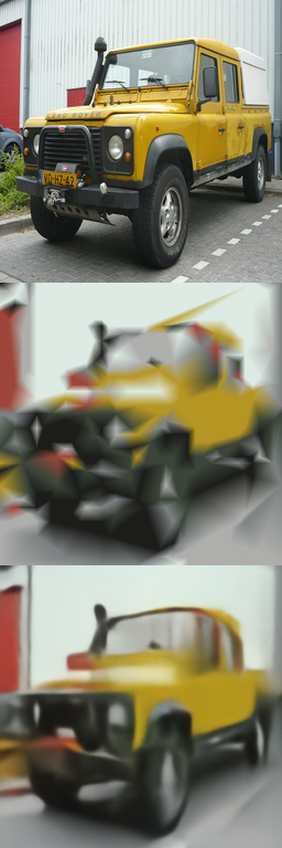
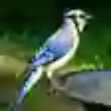
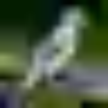
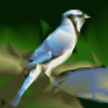
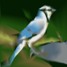
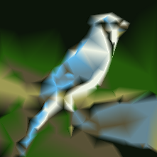
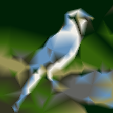
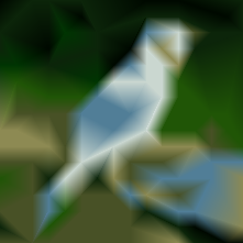
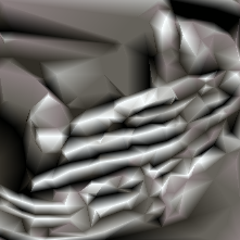
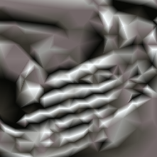
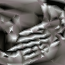
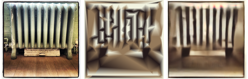
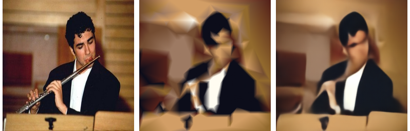
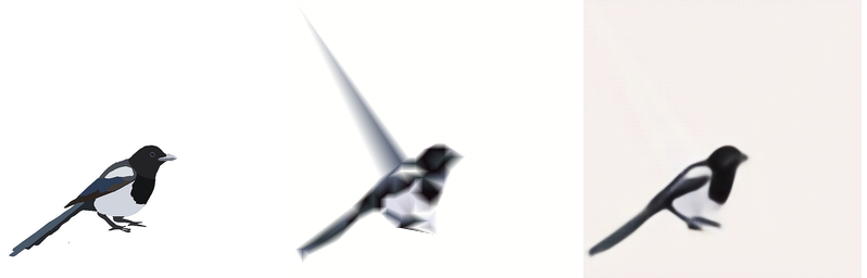
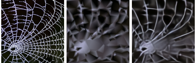
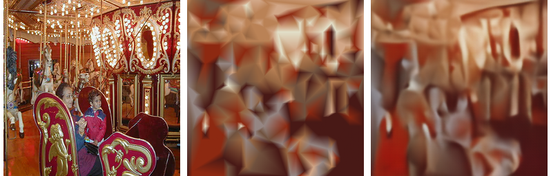
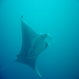
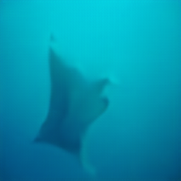
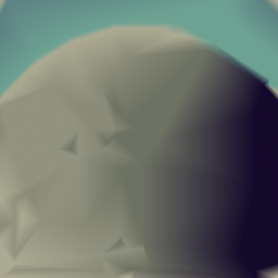
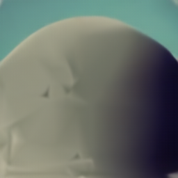
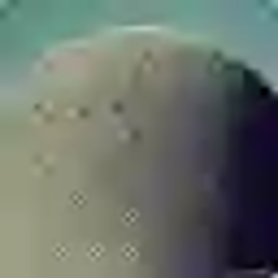
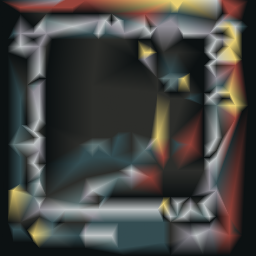
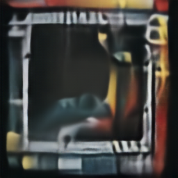
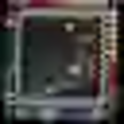
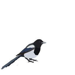
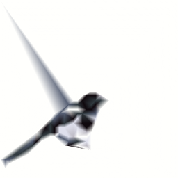
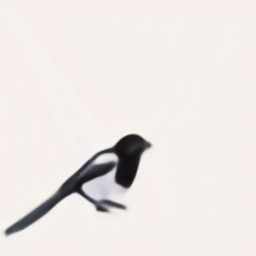
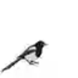
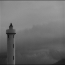
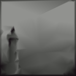
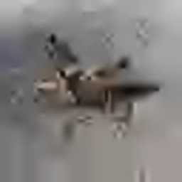
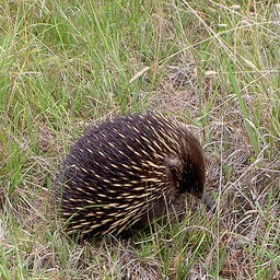
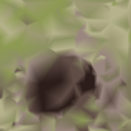
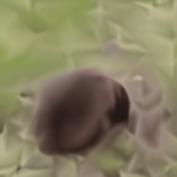
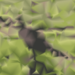
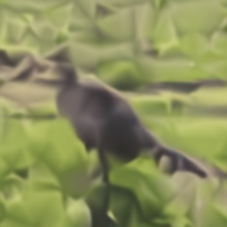
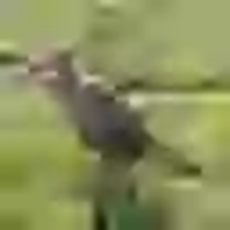
c Network b Triangulation a Original
Reconstruction Reconstruction Image
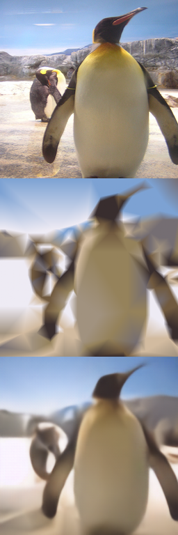
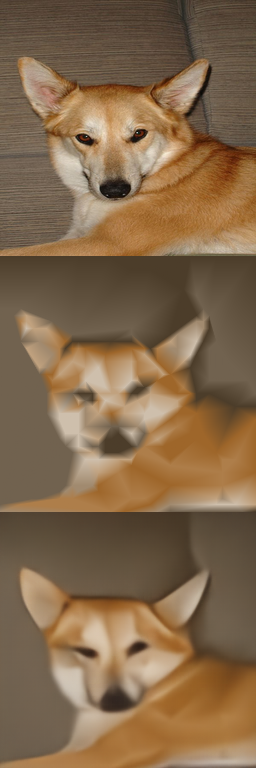
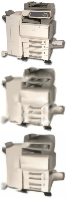

The performance of the triangulation method in [22] provides a strong encoder that works well precisely in the regime of interest: transmission of images under 200 bytes. At that small size, image previews can be easily transmitted as part of the original page-load process on mobile devices or on bandwidth limited connections [6, 22]. When measured in terms of PSNR or SSIM [35], the triangulation method significantly outperformed JPEG and WebP. However, when the images were visually inspected, their visual quality was very uneven: see Figure 1 (row b) for examples. Though some of the images appear very well reconstructed (Figure 1 left columns), others are unrecognizable when viewed without the reference. Other images resulted in spurious edges formed by the triangulation boundaries (Figure 1 right columns). To address these shortcomings, we replace the decoder with a deep convolutional neural network. We ensure that the network remains relatively modest in size for ease of deployment. The decoder input-feature representations played a crucial role for good performance: we provide details in Section 3. The results, presented in Section 4, reveal not only improved PSNR and SSIM scores, but also semantic-content preservation that is quantitatively measured as far superior.
Deep neural networks for compression have been studied in a variety of configurations, from shallow [8, 20, 18] and deep feed-forward auto-encoders [3, 26, 32, 2] to recurrent neural nets/LSTMs for variable-length encodings [33, 34]. Others have taken approaches more closely tied in spirit to ours: employing established encodings as the inputs and using neural networks as the basis for a new decoder with improved performance. These techniques effectively learn a mapping from decompressed patches back to the original image, for example to remove JPEG compression artifacts [37, 30, 7]. Finally, though we do not explore generative adversarial networks (GANs) in this paper, we will briefly address how they can easily be used in a manner similar to other super-resolution and compression studies [21, 1].
2 Triangulation of Images: Encoding & Decoding
In this section, we review the triangulation approach presented in [22]; this yields a state-of-the-art compressed encoding that is used (indirectly) as the input for our neural decoder (presented in the next section).
In [22], the compressed representation of an image describes a list of colored vertices and a color table. The vertices lie on a regular grid of size and the edges of the grid lie on the edges of the image. The vertex color is an index into the color table. Their “triangle-based” decoder constructs a Delaunay triangulation of the vertices on a raster image of size where . Each raster pixel in a triangle is colored using a linear interpolation of the colors of its triangle’s vertices.
Their encoder uses a stochastic-hillclimbing optimizer to find the vertices and color table that optimize the output of their decoder, i.e., that produce a good Delaunay triangulation and raster pixel colors from their decoder algorithm. In this way, the encoder is optimized specifically for their decoder.

86 bytes
76 grid
61 grid
43 grid
33 grid
16 grid
84 bytes
56 grid
33 grid
30 grid
24 grid
15 grid
We built our decoder to directly operate on the output of the state-of-the-art encoder presented in [22] because of its good performance across a wide variety of natural images. and because that encoder has been proposed as a profile in the next-generation WebP standard [23]. By strictly adhering to this as our input with no modifications, wide deployment becomes substantially easier. Ensuring this interoperability of decoders is an important feature since some very low-end devices may not support even our light-weight decoding network; therefore, we need to be able to seamlessly back-off to [22]’s decoder. For those devices that can support forward propagation through our simple network, we will demonstrate substantially improved images in both reconstruction quality and recognizability. Unlike other profile-based compression approaches, this interoperability ensures that the encoder does not need to know which decoder that the client is using. In fact, if necessary, a mix of different decoders can all be supported by exactly the same bit-stream.
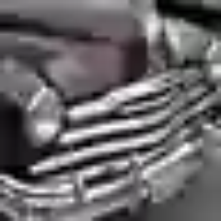
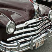
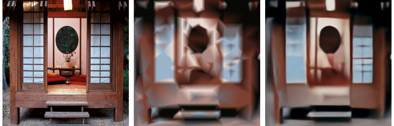
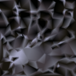
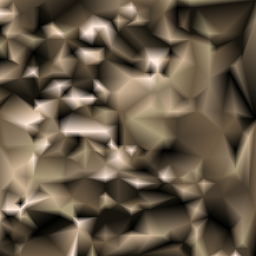
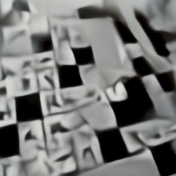
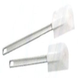
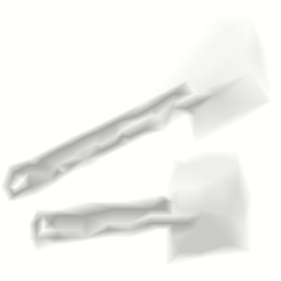
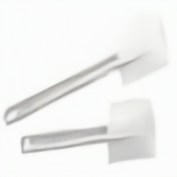
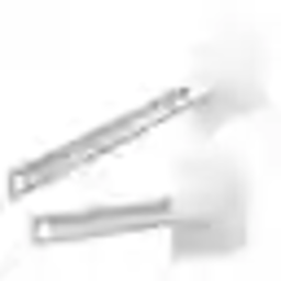
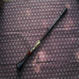
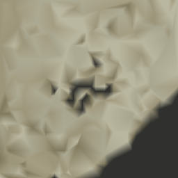
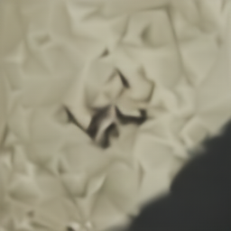
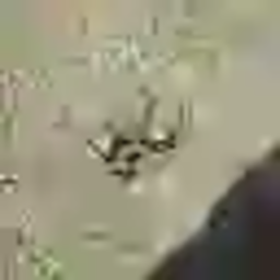
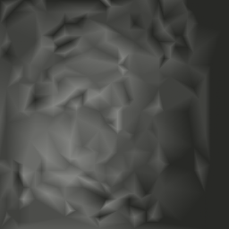
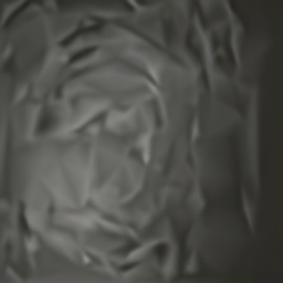
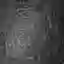
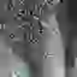
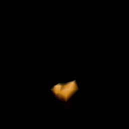
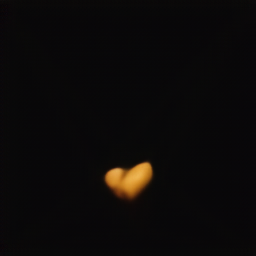
Increasing the vertex grid size (making larger) increases the encoded rate while reducing distortion. Figure 2 shows sample decompressed images with grid sizes ranging from to and compressed sizes ranging from 100 to 400 bytes. In the examples shown in Figure 2, the types of errors that the triangle-shading codec introduces become evident. As each triangle needs to encode more of the image, the jagged edges of the triangles introduce spurious features and misalignments (see the car’s front grill in Figure 2). Nonetheless, it is interesting to note that even at these extreme compression levels many colors and much of the shading remain intact. More examples are presented in Figure 6 and the appendix; see the “interpolated” column.
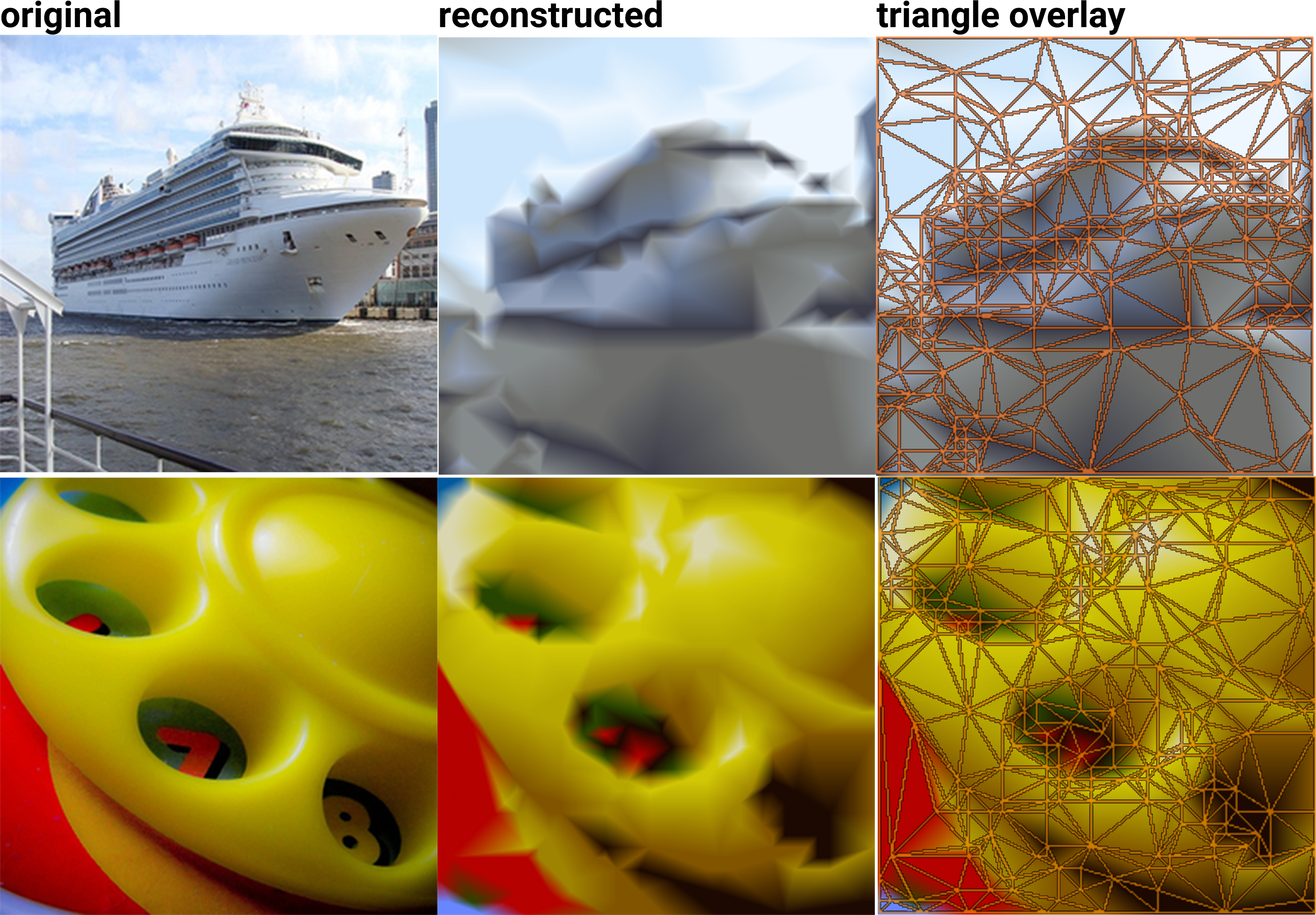
To provide insight into the actual triangulations computed, see Figures 3 (right column) and 4 (“edges” column). As can be seen, triangles are more densely concentrated in the high-entropy regions of the image. In contrast, the uniform regions of the input image are adequately represented by fewer triangles.
3 Neural Decoding
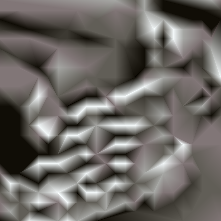
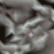
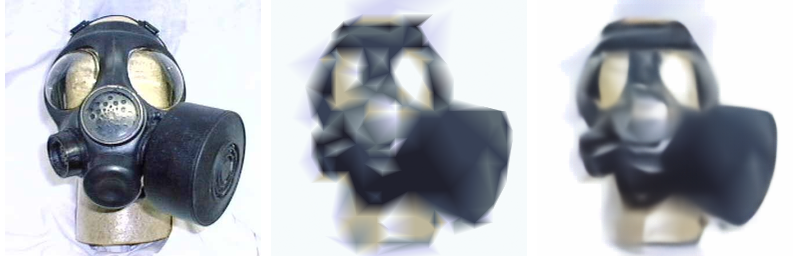
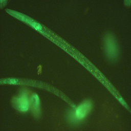
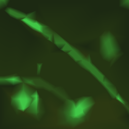
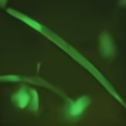
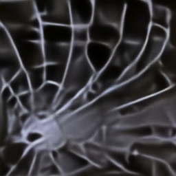
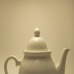
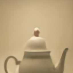
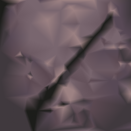
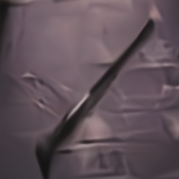
Let us examine a few sample triangulations in detail to see where there is room for improvement: see Figure 3. The most salient observations are: (1) there are severe jagged edges in the image (see both images) and (2) discontinuities in straight lines appear (see the boat-deck outline). These are caused by triangle boundaries. Recall that each triangle is in-painted using only the colors of its own vertices. However, vertices of nearby triangles have the potential to contain valuable information - especially when they are assigned the same (or nearly same) color. For example, in the toy-dial image, notice that many triangles encode subtle shading differences. It should be possible to use this consistency information across triangles in re-rendering the image.
One can imagine a variety of simple techniques to overcome the jagged edges in the decoded image. However, designing the rules to best employ information from close triangles will likely result in a number of ad-hoc heuristics and thresholds. Instead, we use a deep neural network to implicitly create the rules to address both of these shortcomings, based on image statistics. To train the network, we start with exactly the same inputs from the triangulation procedure that were used to render the images shown above. For the target output, we use the original image. Training proceeds using samples from Imagenet’s training set [28].
3.1 Architecture and Inputs
A variety of deep convolutional networks have been driving recent computer-vision research, for example in object detection and recognition (e.g. the Imagenet challenge [28] and activity recognition [29]). For this application, however, the goal is to take an extremely sparse input and generate a full image. We formulate this problem as an image-translation task. As described by Isola et. al., Image translation is the task of “translating one possible representation of a scene into another, given sufficient training data … the setting is always the same: predict pixels from pixels” [17].
Unlike the more common object-identification tasks, where the end result is a classification, here the result is a full image. Therefore, it is important to be able to recreate details from the inputs while allowing for non–spatially-local influences to direct larger features and impose global consistency. The need to have both details from the original image and potentially global coordination of the generated image has resulted in a variety of finecoarsefine architectures such as “hourglass” and “u-net” [17, 27]. These architectures pass the inputs through a series of convolution layers that progressively downsample the image. After the smallest layer is reached, the process is reversed and the image is expanded back to the desired size.
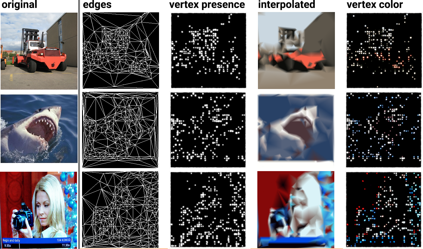
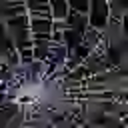
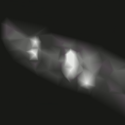
One of the largest differences between the previous image-to-image translation work and ours is that our inputs are not the typical 3-channel images. Instead, they are composed of 8 channels (Figure 4): (channel 1) the edge image - a binary image showing the edges created by the Delaunay triangulation; (channel 2) the binary vertex-presence image; (channels 3-5) the reconstruction using the original system’s bilinear-interpolation approach [22]; and (channels 6-8) the RGB color-vertex image showing the color assigned to each vertex (with black everywhere else).111The decision to use images as inputs into the network is not the only possible approach. For example, after decoding the transmission, the series of vertex+color tuples could be directly used. We did not pursue this avenue since, in addition to learning the image-translation problem, it would require the network to learn how to triangulate and how to map between the real-value inputs and coordinates. Further, more complex measures would be required to handle the variable number of vertices. All of these are avoided by using the eight-channel, image-like input in which the spatial information is explicitly maintained and the triangulation’s edges directly given.
Beyond good reconstruction performance, an equally important consideration for this study was the simplicity/size of the final decoding network — keeping computation requirements manageable is crucial for large-scale device deployment. An enormous number of architectures and a variety of approaches were empirically examined. Because of space limitations, we provide a brief summary of them here. We tried architectures ranging from image-translation (e.g. pix2pix [17], cycle-gan [38]), to shape-encoding/decoding networks (e.g., where the bottleneck is a set of geometric descriptions), to progressive-completion networks [33, 34]. The approach that provided the best trade-off, in terms of reconstruction quality vs. simplicity, was the stacked hourglass network described below. The hourglass network is also simple enough to meet the NBU-application’s requirements since, in NBU areas, processor computational limitations are prevalent in the available mobile devices. As a secondary benefit, the number of hourglass networks (e.g. stack size) can be adjusted according to computational availability, though, as will be described in the experiments, even a single hourglass provides substantial benefits.
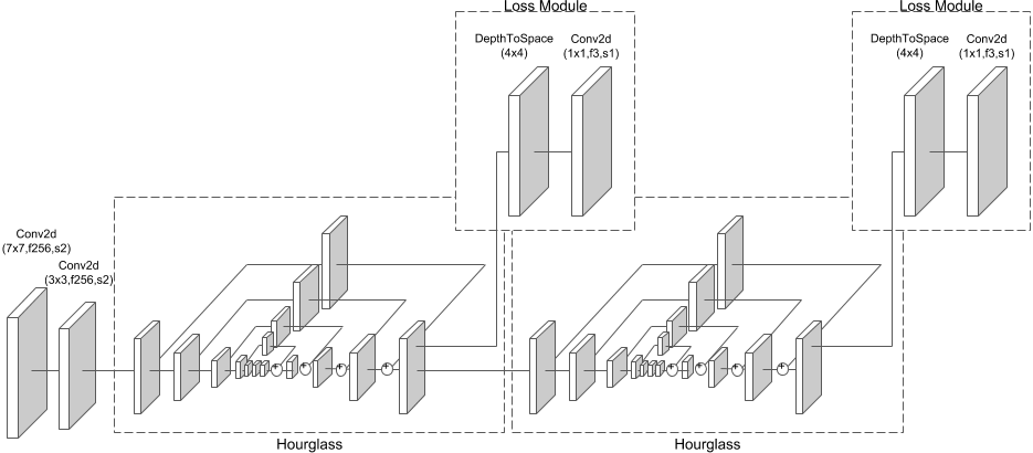
The remainder of this study uses the most promising of these: the hourglass network. The input images have a resolution of with 8 channels and a batch size of 32. The output is an RGB image of the same resolution. Our network (Figure 5) is based on the Stacked Hourglass in [24]. We apply a Conv2d(size=7x7,filters=256,stride=2) to the input, then a Conv2d(3x3,f256,s2) to bring the dimensions to . This feeds into an Hourglass as described in [24] except 1) when downscaling, each MaxPool layer is replaced by a layer that stacks the values of each spatial block depth-wise (a SpaceToDepth(2x2) layer) followed by a Conv2d(3x3,f256,s1) and, 2) when upscaling, each nearest neighbor upsampling is replaced by a DepthToSpace(2x2), the inverse of a SpaceToDepth, followed by a Conv2d(3x3,f256,s1). The Hourglass output is added to the Hourglass input and passed to the next Hourglass. We stacked two Hourglass networks.
To apply intermediate supervision as described in [24], we split an intermediate Loss Module off the output of every Hourglass. It is a DepthToSpace(4x4) and a Conv2d(1x1,f3,s1) with a Tanh activation to get us to a RGB image. During training, we apply a mean-squared-error loss between this and the original ground truth image to maximize PSNR. During inference, the network’s prediction is the RGB image in the second (final) Hourglass’s Loss Module. Every layer is followed by Batch Norm and Relu except the final layer (with the Tanh). We use the Adam Optimizer [19] with learning rate of 0.1.
4 Experimental Results
The network described in the previous section was trained for 2.2 million steps on five asynchronous GPUs: this was approximately 15 days of continuous training. Testing was conducted on 20,000 images drawn from the ImageNet validation set; these were not used elsewhere in training.
Detailed notes:
A: Note the jagged lines along the window.
B: Both images are recognizable, but our method provides cleaner lines.
C: Note the severe artifacts in the vertical lines.
D: Note the smooth shading from the lights and the hair lines.
E: Note the problem with the two thin triangles starting from the upper left corner.
F: Neither method provides a good reconstruction but our decoder gives a slightly better rendition.
G: Compression rate is too extreme for either method to provide recognizable results.
original interp. [22] neural (ours) interp. v nn
A.
 PSNR: 17.74 v 19.00
SSIM: 0.39 v 0.46
B.
 PSNR: 18.01 v 19.46
SSIM: 0.48 v 0.54
C.
 PSNR: 14.67 v 18.03
SSIM: 0.42 v 0.48
D.
 PSNR: 21.54 v 23.44
SSIM: 0.73 v 0.78
E.
 PSNR: 21.47 v 22.90
SSIM: 0.90 v 0.96
F.
 PSNR: 11.66 v 12.12
SSIM: 0.15 v 0.24
G.
 PSNR: 15.86 v 16.19
SSIM: 0.21 v 0.24
In addition to Figure 1, Figure 6 and the appendix provide more comparisons to the interpolated images and their respective PSNR and SSIM (Structural Similarity Index [35]) scores. Overall, when measured on the entire testing set, we are able to outperform the triangulation approaches in both PSNR and SSIM.
-
•
For PSNR: Triangulation scored 20.7 dB and our neural approach scored 21.7 dB. In this range, a 1-dB PSNR increase is extremely valuable. Out of the 13,000 examples examined, 12,810 (98.5%) showed improved PSNR via the neural decoding. Comparing the two approaches using a standard -test on the PSNR, .
-
•
For SSIM: Triangulation scored 0.51 and our neural approach scored 0.54. Out of the 13,000 examples examined, 12,255 (94.2%) were improved via the neural decoding. Comparing the two approaches using a standard -test on SSIM, .
Importantly, recall that the triangulation method [22] also outperformed JPEG and WebP, which, in turn, equals or outperforms JPEG2000 [12, 14].
To better understand what the network was encoding, an extensive grid search was also performed to determine which channels were actually necessary. For space reasons, we cannot recreate all of the results here. A few salient findings, however, are worth noting: (1) The best performing network was one that received all the eight channels as input; (2) If we removed the interpolated image (as created by [22]) from the inputs, the PSNR performance drops approximately 0.75 dB; (3) Interestingly, if we used only the interpolated as input, the PSNR performance drops 0.5 dB; (4) Finally, while we used 2 stacked Hourglasses in this work, the results with 1 Hourglass or 3 stacked Hourglasses were almost identical; any variation was likely due to the stochasticity in the training procedure. On a mobile or computationally constrained device, a single Hourglass can be used. This decision on the complexity of the decoder can be made on a pre-device basis and all will work on exactly the same encoding.
4.1 Semantic Content Preservation
The quantitative results, in terms of PSNR and SSIM, reveal a significant improvement for extremely compressed images. Despite the numeric improvements, however, it is important to assess whether the images are qualitatively better. The simplest, though resource-consuming, method is to employ human raters. We propose a novel technique using a well-trained classification network as an automated proxy.
| (Lower Better) | (Higher Better) | |||
|---|---|---|---|---|
| Error | Recall Top-1 | Recall Top-5 | Recall Top-10 | |
| interpolated [22] | 39.5 | 0.05 | 0.13 | 0.15 |
| nn-Decoded (our method) | 36.0 | 0.17 | 0.33 | 0.38 |
| interpolated+Blur x1 | 39.5 | 0.11 | 0.26 | 0.30 |
| interpolated+Blur x5 | 43.0 | 0.08 | 0.18 | 0.22 |
For our experiments, we employ a pre-trained state-of-the-art classifier, Inception ResNet v2 (IR2), which produces a 1000-dimension “classification vector” prior to the final soft-max layer representing the classification of the objects in the image. On the ImageNet challenge, IR2 has has a top-1 single-crop error rate of 19.9% on the 50,000 image validation set, and a top-5 error rate of 4.9% [31]. For each of our test images, we use the original image, the interpolated image and the neural decoded image: , , and . Passing each of these through IR2 produces classification vectors , , and . We measure the similarity between and and between and in two ways: (1) the difference between the classification vectors, and (2) whether the top classification in appears in the top-1, -5, and -10 positions of and .
Note that this is not equivalent to checking the ground-truth classification. The goal of our compression task is not to alter the original image to make a wrong classification correct, it is to achieve the same classification as the original. Finally, we remark that with such aggressive compression rates, we do not expect all images to be recognized; for example, images in which the object of interest does not cover a large portion of the image, the object may be lost. Nonetheless, for images in which the object is large, these metrics elucidate how recognizable the object remains.
The results are presented in the first two rows of Table 1. There is more than a 10% decrease in the error using the neural-network decoding. However, the largest benefit comes when looking at the recall measures. Looking at recall in the top-1 position, the results are 300% improved (3) and at top-10, they remain approximately 2.5 improved. This large gain indicates that the content of the image remains far more recognizable using our neural-network decoder.
Upon first glance at our decoded neural-network images, it is tempting to wonder if much of the recognition improvement is coming from simply blurring the triangulated image. Though we would not expect an improvement in PSNR or SSIM from additional blurring, it is possible that the Inception-Resnet-V2 network is not robust to the types of edges seen in Figure 6. We explicitly checked that possibility, to ensure that the network is not acting as an overly complex approach to a simple blur operation. Instead of decoding with a neural network, we use the method from [22] followed by Gaussian blurring (=2). We create two new test sets: the first with a single pass of a blur filter and the second with 5 sequential passes. The last two rows of Table 1 show the performance after the added blurring. The results, though improved, do not match those our NN-based decoding. And, as expected, the PSNR and SSIM rates decline for both sets over the base triangulation results reported above (PSNR: blur1: 20.6, blur5: 19.6, SSIM: blur1: 0.50, blur5: 0.46). Visually, it appears that the neural approach is smoothing the harsh color transitions created by the triangulation. However, based on the PSNR/SSIM scores and the similarity of the classification vectors, the neural network’s effect is well targeted: the edges and details required to maintain the object identity and similarity to the original image are preserved.
5 Discussion & Future Work
The application of neural networks to image decompression is not only of interest to researchers and practitioners, as witnessed by the vast amount of neural image compression literature, but also will have a large and socially important impact: allowing efficient discovery/browsing of visual content for the “next-billion users” whose bandwidth is limited and expensive. We have found that the impact of using neural networks in place of the current triangle-shading decoder results in consistent and very significant quantitative and qualitative improvements to the final image quality.
By casting the task of decompression into an image-to-image–translation problem, we were able to generate images that, when compared to recently released state-of-the-art compression techniques, more closely resemble the original image in terms of the standard quantitative metrics such as PSNR and SSIM. More importantly, they far exceeded the previous method [22] in preserving semantic quality. The results come in an operating regime of extreme compression where there is large practical interest, but existing compression schemes do not fare well.
These improved results are somewhat surprising since, on each encoding, the encoder is explicitly optimizing for the best results from the triangle-based decoder in [22]. Yet, we are able to provide better reconstructions with neural decompression without changing the encoder at all. This points the way for efforts to replace full H.264 decoders with neural approaches without changing the already deployed video encoders.
This study leads to many avenues of future work. First, simultaneously to the development of this study, Generative Adversarial Networks were in parallel developed for compression [1]. Beyond using GANs for error signals, they also make clever use of the ability for GANs to synthesize, rather than compress. Though they operate on larger images at higher bit rates, many of the same approaches, including using GANs to augment the objective functions, can easily be incorporated.
Second, although not discussed in this paper, an interesting side finding was early evidence that it is possible to train a network to infer a Delaunay triangulation given just the vertex points. In preliminary studies, the network fared much better than expected in not only finding the same connections, but also in creating relatively straight edges between the vertices (the output was a image). If these results hold true, this has potentially broad applicability as the operation of triangulation could then be integrated into a fully differentiable system.
Third, we should consider that if we know that semantic recall, as measured by IR2, is important, should it be included as an extra error term during training? The answer may not be straightforward – if it is used, it is possible that the examples generated will take advantage of small inconsistencies in the training, in the same way that adversarial attacks are remarkably plentiful and easy to find. On the other hand, if we train and test on distinct semantic models, perhaps the semantic recall will improve without falling into model-specific traps.
References
- [1] E. Agustsson, M. Tschannen, F. Mentzer, R. Timofte, and L. V. Gool. Generative adversarial networks for extreme learned image compression. CoRR, abs/1804.02958, 2018.
- [2] J. Ballé, V. Laparra, and E. P. Simoncelli. End-to-end optimized image compression. In Int’l. Conf. on Learning Representations (ICLR2017), Toulon, France, April 2017. Available at http://arxiv.org/abs/1611.01704.
- [3] J. Ballé, D. Minnen, S. Singh, S. J. Hwang, and N. Johnston. Variational image compression with a scale hyperprior. arXiv preprint arXiv:1802.01436, 2018.
- [4] S. Bougleux, G. Peyré, and L. D. Cohen. Image compression with anisotropic triangulations. In Computer Vision, 2009 IEEE 12th International Conference on, pages 2343–2348. IEEE, 2009.
- [5] O. Bryt and M. Elad. Compression of facial images using the K-SVD algorithm. Journal of Visual Communication and Image Representation, 19(4):270–282, 2008.
- [6] B. Cabral and E. Kandrot. The technology behind preview photos. https://code.facebook.com/ posts/991252547593574/the-technology-behind-preview-photos/, 2015.
- [7] L. Cavigelli, P. Hager, and L. Benini. Cas-cnn: A deep convolutional neural network for image compression artifact suppression. In Neural Networks (IJCNN), 2017 International Joint Conference on, pages 752–759. IEEE, 2017.
- [8] G. W. Cottrell and P. Munro. Principal components analysis of images via back propagation. In Visual Communications and Image Processing’88: Third in a Series, volume 1001, pages 1070–1078. International Society for Optics and Photonics, 1988.
- [9] F. Davoine, M. Antonini, J.-M. Chassery, and M. Barlaud. Fractal image compression based on delaunay triangulation and vector quantization. IEEE Transactions on Image Processing, 5(2):338–346, 1996.
- [10] B. Delaunay. Sur la sphere vide. Izv. Akad. Nauk SSSR, Otdelenie Matematicheskii i Estestvennyka Nauk, 7(793-800):1–2, 1934.
- [11] L. Demaret, N. Dyn, and A. Iske. Image compression by linear splines over adaptive triangulations. Signal Processing, 86(7):1604–1616, 2006.
- [12] G. Developers. Comparative study of webp, jpeg and jpeg 2000. https://developers.google.com/speed/webp/docs/c_study, 2010.
- [13] G. Developers. A new image format for the web. https://developers.google.com/speed/webp/, 2016.
- [14] G. Developers. Webp compression study. https://developers.google.com/speed/webp/docs/webp_study, 2016.
- [15] B. Huang. Satellite data compression. Springer Science & Business Media, 2011.
- [16] A. Inc. Using HEIF or HEVC media on Apple devices. https://support.apple.com/en-us/HT207022, 2017.
- [17] P. Isola, J.-Y. Zhu, T. Zhou, and A. A. Efros. Image-to-image translation with conditional adversarial networks. arXiv preprint, 2017.
- [18] J. Jiang. Image compression with neural networks–a survey. Signal Processing: Image Communication, 14(9):737–760, 1999.
- [19] D. P. Kingma and J. Ba. Adam: A method for stochastic optimization. April 2014. Available at http://arxiv.org/abs/1412.6980.
- [20] M. A. Kramer. Nonlinear principal component analysis using autoassociative neural networks. AIChE journal, 37(2):233–243, 1991.
- [21] C. Ledig, L. Theis, F. Huszár, J. Caballero, A. Cunningham, A. Acosta, A. Aitken, A. Tejani, J. Totz, Z. Wang, et al. Photo-realistic single image super-resolution using a generative adversarial network. arXiv preprint, 2016.
- [22] D. Marwood, P. Massimino, M. Covell, and S. Baluja. Representing images in 200 bytes: Compression via triangulation. In International Conference On Image Processing, 2018 (arxiv:1809.02257).
- [23] P. Massimino. Re: Questions about plans for the triangle encoder going into next-gen WebP. e-mail communication, 2018.
- [24] A. Newell, K. Yang, and J. Deng. Stacked hourglass networks for human pose estimation. In European Conference on Computer Vision, pages 483–499. Springer, 2016.
- [25] A. Orzan, A. Bousseau, P. Barla, H. Winnemöller, J. Thollot, and D. Salesin. Diffusion curves: a vector representation for smooth-shaded images. Communications of the ACM, 56(7):101–108, 2013.
- [26] O. Rippel and L. Bourdev. Real-time adaptive image compression. In International Conference on Machine Learning (ICML), 2017. IEEE, 2017.
- [27] O. Ronneberger, P. Fischer, and T. Brox. U-net: Convolutional networks for biomedical image segmentation. In International Conference on Medical image computing and computer-assisted intervention, pages 234–241. Springer, 2015.
- [28] O. Russakovsky, J. Deng, H. Su, J. Krause, S. Satheesh, S. Ma, Z. Huang, A. Karpathy, A. Khosla, M. S. Bernstein, A. C. Berg, and F. Li. Imagenet large scale visual recognition challenge. CoRR, abs/1409.0575, 2014.
- [29] K. Simonyan and A. Zisserman. Two-stream convolutional networks for action recognition in videos. In Advances in neural information processing systems, pages 568–576, 2014.
- [30] P. Svoboda, M. Hradis, D. Barina, and P. Zemcík. Compression artifacts removal using convolutional neural networks. CoRR, abs/1605.00366, 2016.
- [31] C. Szegedy, S. Ioffe, V. Vanhoucke, and A. Alemi. Inception-v4, inception-resnet and the impact of residual connections on learning. arXiv preprint arXiv:1602.07261, 2016.
- [32] L. Theis, W. Shi, A. Cunningham, and F. Huszár. Lossy image compression with compressive autoencoders. In International Conference on Learning Representations, 2017.
- [33] G. Toderici, S. M. O’Malley, S. J. Hwang, D. Vincent, D. Minnen, S. Baluja, M. Covell, and R. Sukthankar. Variable rate image compression with recurrent neural networks. ICLR, 2016.
- [34] G. Toderici, D. Vincent, N. Johnston, S. J. Hwang, D. Minnen, J. Shor, and M. Covell. Full resolution image compression with recurrent neural networks. In Computer Vision and Pattern Recognition (CVPR), 2017 IEEE Conference on, pages 5435–5443. IEEE, 2017.
- [35] Z. Wang, A. C. Bovik, H. R. Sheikh, and E. P. Simoncelli. Image quality assessment: from error visibility to structural similarity. IEEE transactions on image processing, 13(4):600–612, 2004.
- [36] Y. Watkins, M. Sayeh, O. Iaroshenko, and G. Kenyon. Image compression: Sparse coding vs. bottleneck autoencoders. CoRR, abs/1710.09926, 2017.
- [37] K. Yu, C. Dong, C. C. Loy, and X. Tang. Deep convolution networks for compression artifacts reduction. arXiv preprint arXiv:1608.02778, 2016.
- [38] J.-Y. Zhu, T. Park, P. Isola, and A. A. Efros. Unpaired image-to-image translation using cycle-consistent adversarial networks. arXiv preprint, 2017.
- [39] J.-Y. Zhu, Z.-Y. Wang, R. Zhong, and S.-M. Qu. Dictionary based surveillance image compression. Journal of Visual Communication and Image Representation, 31:225–230, 2015.
Appendix A Additional Examples
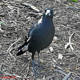
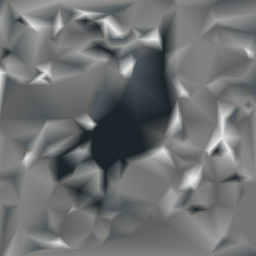
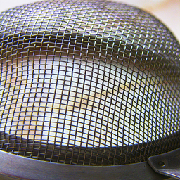
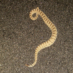
We provide additional examples of the neural-decoding method’s best and worst performance on both PSNR and SSIM. Images are from the ImageNet test set, reported in the paper.
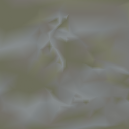
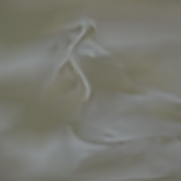
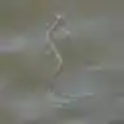
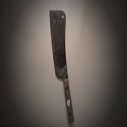
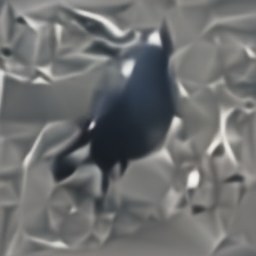
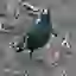
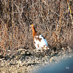
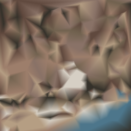
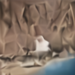
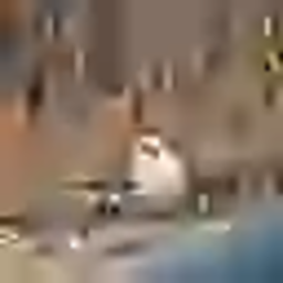
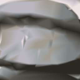
Ten examples of each have been provided in the tables below along with their metrics and a comparison to the bi-linear–interpolated, non–neural-network approach and WebP. Because WebP could not target the same rates on resolution images, the input images were resized to 4 or more times smaller in each dimension, compressed with WebP, decompressed, and then upscaled to bring it back to source resolution.
| Original Image | Interpolated | Neural Decoded | WebP |
 |
 |
 |
 |
| Ground Truth | 33.0163 PSNR, 0.9023 SSIM | 34.2382 PSNR, 0.9074 SSIM | 28.8307 PSNR, 0.8653 SSIM |
 |
 |
 |
 |
| Ground Truth | 32.3473 PSNR, 0.9331 SSIM | 34.7422 PSNR, 0.9415 SSIM | 33.7351 PSNR, 0.9364 SSIM |
 |
 |
 |
 |
| Ground Truth | 32.7623 PSNR, 0.9441 SSIM | 34.8865 PSNR, 0.9535 SSIM | 37.6550 PSNR, 0.9625 SSIM |
 |
 |
 |
 |
| Ground Truth | 29.7310 PSNR, 0.9296 SSIM | 35.3078 PSNR, 0.9522 SSIM | 33.9794 PSNR, 0.9413 SSIM |
 |
 |
 |
 |
| Ground Truth | 36.9100 PSNR, 0.9358 SSIM | 37.3513 PSNR, 0.8361 SSIM | 36.0570 PSNR, 0.8978 SSIM |
| Original Image | Interpolated | Neural Decoded | WebP |
 |
 |
 |
 |
| Ground Truth | 33.5368 PSNR, 0.9082 SSIM | 34.4789 PSNR, 0.9242 SSIM | 33.0402 PSNR, 0.9024 SSIM |
 |
 |
 |
 |
| Ground Truth | 34.2424 PSNR, 0.8959 SSIM | 34.8164 PSNR, 0.9018 SSIM | 33.2535 PSNR, 0.8920 SSIM |
 |
 |
 |
 |
| Ground Truth | 30.6643 PSNR, 0.9273 SSIM | 34.9344 PSNR, 0.9540 SSIM | 31.6522 PSNR, 0.9306 SSIM |
 |
 |
 |
 |
| Ground Truth | 34.7180 PSNR, 0.9317 SSIM | 35.7485 PSNR, 0.9376 SSIM | 33.5282 PSNR, 0.9195 SSIM |
 |
 |
 |
 |
| Ground Truth | 41.7112 PSNR, 0.9772 SSIM | 37.4974 PSNR, 0.9389 SSIM | 41.7442 PSNR, 0.9762 SSIM |
| Original Image | Interpolated | Neural Decoded | WebP |
 |
 |
 |
 |
| Ground Truth | 11.6645 PSNR, 0.1480 SSIM | 12.1248 PSNR, 0.2400 SSIM | 11.8997 PSNR, 0.1747 SSIM |
 |
 |
 |
 |
| Ground Truth | 13.2179 PSNR, 0.2111 SSIM | 13.2259 PSNR, 0.2121 SSIM | 13.2145 PSNR, 0.2086 SSIM |
 |
 |
 |
 |
| Ground Truth | 13.2704 PSNR, 0.3395 SSIM | 13.3209 PSNR, 0.3734 SSIM | 12.8824 PSNR, 0.2858 SSIM |
 |
 |
 |
 |
| Ground Truth | 13.0367 PSNR, 0.1830 SSIM | 13.4482 PSNR, 0.2189 SSIM | 12.6962 PSNR, 0.1356 SSIM |
 |
 |
 |
 |
| Ground Truth | 12.7520 PSNR, 0.2868 SSIM | 13.5967 PSNR, 0.3586 SSIM | 12.4848 PSNR, 0.2032 SSIM |
| Original Image | Interpolated | Neural Decoded | WebP |
 |
 |
 |
 |
| Ground Truth | 12.0996 PSNR, 0.2213 SSIM | 12.8032 PSNR, 0.3029 SSIM | 11.6907 PSNR, 0.1503 SSIM |
 |
 |
 |
 |
| Ground Truth | 13.1227 PSNR, 0.1299 SSIM | 13.2882 PSNR, 0.1496 SSIM | 13.0452 PSNR, 0.1211 SSIM |
 |
 |
 |
 |
| Ground Truth | 13.2473 PSNR, 0.1040 SSIM | 13.4038 PSNR, 0.1157 SSIM | 13.1843 PSNR, 0.0973 SSIM |
 |
 |
 |
 |
| Ground Truth | 13.3954 PSNR, 0.1427 SSIM | 13.4994 PSNR, 0.1541 SSIM | 13.4025 PSNR, 0.1437 SSIM |
 |
 |
 |
 |
| Ground Truth | 13.1887 PSNR, 0.2672 SSIM | 13.6563 PSNR, 0.3064 SSIM | 11.8838 PSNR, 0.1647 SSIM |
| Original Image | Interpolated | Neural Decoded | WebP |
 |
 |
 |
 |
| Ground Truth | 23.0814 PSNR, 0.9077 SSIM | 27.0714 PSNR, 0.9474 SSIM | 23.4490 PSNR, 0.9231 SSIM |
 |
 |
 |
 |
| Ground Truth | 30.5001 PSNR, 0.9176 SSIM | 32.3672 PSNR, 0.9495 SSIM | 30.8484 PSNR, 0.9180 SSIM |
 |
 |
 |
 |
| Ground Truth | 29.7310 PSNR, 0.9296 SSIM | 35.3078 PSNR, 0.9522 SSIM | 33.9794 PSNR, 0.9413 SSIM |
 |
 |
 |
 |
| Ground Truth | 30.6643 PSNR, 0.9273 SSIM | 34.9344 PSNR, 0.9540 SSIM | 31.6522 PSNR, 0.9306 SSIM |
 |
 |
 |
|
| Ground Truth | 31.1331 PSNR, 0.9571 SSIM | 31.7848 PSNR, 0.9567 SSIM | 31.6693 PSNR, 0.9548 SSIM |
| Original Image | Interpolated | Neural Decoded | WebP |
 |
 |
 |
 |
| Ground Truth | 29.5948 PSNR, 0.9361 SSIM | 31.0210 PSNR, 0.9480 SSIM | 30.1475, 0.9384 SSIM |
 |
 |
 |
 |
| Ground Truth | 31.7642 PSNR, 0.9299 SSIM | 34.0957 PSNR, 0.9505 SSIM | 32.7695 PSNR, 0.9360 SSIM |
 |
 |
 |
 |
| Ground Truth | 32.7623 PSNR, 0.9441 SSIM | 34.8865 PSNR, 0.9535 SSIM | 37.6550 PSNR, 0.9625 SSIM |
 |
 |
 |
 |
| Ground Truth | 21.4695 PSNR, 0.8972 SSIM | 22.9038 PSNR, 0.9565 SSIM | 25.5479 PSNR, 0.9398 SSIM |
 |
 |
 |
 |
| Ground Truth | 25.5729 PSNR, 0.9287 SSIM | 33.2967 PSNR, 0.9612 SSIM | 26.4886 PSNR, 0.9374 SSIM |
| Original Image | Interpolated | Neural Decoded | WebP |
 |
 |
 |
 |
| Ground Truth | 15.5495 PSNR, 0.0659 SSIM | 15.6083 PSNR, 0.0734 SSIM | 15.5354 PSNR, 0.0735 SSIM |
 |
 |
 |
 |
| Ground Truth | 16.5936 PSNR, 0.0833 SSIM | 16.7179 PSNR, 0.0909 SSIM | 16.5516 PSNR, 0.0860 SSIM |
 |
 |
 |
 |
| Ground Truth | 16.4997 PSNR, 0.0879 SSIM | 16.5101 PSNR, 0.0944 SSIM | 16.4033 PSNR, 0.08411 SSIM |
 |
 |
 |
 |
| Ground Truth | 18.2631 PSNR, 0.0962 SSIM | 18.3455 PSNR, 0.1022 SSIM | 18.0795 PSNR, 0.0917 SSIM |
 |
 |
 |
 |
| Ground Truth | 16.6109 PSNR, 0.1014 SSIM | 16.7528 PSNR, 0.1111 SSIM | 16.4989 PSNR, 0.0962 SSIM |
| Original Image | Interpolated | Neural Decoded | WebP |
 |
 |
 |
 |
| Ground Truth | 16.0347 PSNR, 0.0777 SSIM | 16.1087 PSNR, 0.0814 SSIM | 15.9726 PSNR, 0.0765 SSIM |
 |
 |
 |
 |
| Ground Truth | 17.7205 PSNR, 0.0933 SSIM | 17.7716 PSNR, 0.0935 SSIM | 17.7348 PSNR, 0.0909 SSIM |
 |
 |
 |
 |
| Ground Truth | 13.4859 PSNR, 0.0805 SSIM | 13.6928 PSNR, 0.1000 SSIM | 13.4264 PSNR, 0.0754 SSIM |
 |
 |
 |
 |
| Ground Truth | 33.1259 PSNR, 0.9421 SSIM | 28.6035 PSNR, 0.1032 SSIM | 34.9583 PSNR, 0.9679 SSIM |
 |
 |
 |
 |
| Ground Truth | 16.5107 PSNR, 0.1072 SSIM | 16.6494 PSNR, 0.1148 SSIM | 16.0610 PSNR, 0.0815 SSIM |