Anti-Chaos Control via Nonlinear Schrödinger Equations for the secured optical communication

Abstract

Coupled nonlinear Schrödinger equations, governing the propagation of envelopes of electromagnetic waves in birefringent optical fibers, are studied in this paper for their potential applications in the secured optical communication. Periodicity and integrability of the CNLS equations are obtained via the phase-plane analysis. With the time-delay and perturbations introduced, CNLS equations are chaotified and a chaotic system is proposed. Numerical and analytical methods are conducted on such system: (I) Phase projections are given and the final chaotic states can be observed. (II) Power spectra and the largest Lyapunov exponents are calculated to corroborate that those motions are indeed chaotic.


Keywords: Chaotification; Couple nonlinear Schrödinger equations; Chaotic Motion; Time delay

Interest in the optical solitons has grown for their potential applications in the telecommunications and ultrafast signal routing systems, especially the vector ones beijingsoliton1 ; beijingsoliton2 . The coupled nonlinear Schrödinger (CNLS) equations, which can be used to govern the propagation of envelopes of electromagnetic waves in birefringent optical fibers, read as source1 ; source2 ,

$$iu_{x}+u_{tt}+2\kappa(|u|^{2}+|v|^{2})u=0,$$ (1)

$$iv_{x}+v_{tt}+2\kappa(|u|^{2}+|v|^{2})v=0,$$ (2)

where $u$ and $v$, two complex functions about $x$ and $t$, are the normalized envelopes of the optical pulses along the two circularly polarized modes of a birefringent optical fiber, $x$ represents the normalized distance along the direction of propagation, $t$ refers to the retarded time, and $\kappa$ gives the strength of the nonlinearity source1 ; source2 . Some studies on Eqs. (1) have been investigated in the early literatures, e.g., the bright soliton solutions done1 , dark soliton solutions done2 and the effects of noise on the solitons done3 .

Chaotic dynamics, owing to its noise-like broadband power spectra, is a good candidate to fight narrow-band effects, such as the frequency-selective fading or narrow-band disturbances in the communication systems secure3 ; secure4 . Thus, for the secured optical communication, chaotic signals have received increasing attention because of their dependence on the initial condition, which makes it difficult to guess the structure of the generator and to predict the signal over a longer time interval secure1 ; secure2 . Therefore, as opposed to controlling or eliminating chaos in dynamical systems control , creating chaos from a non-chaotic system attracts some interests for the secured optical communication and information security chaotification1 . People have known that a system with time-delay is inherently infinite dimensional, so it can produce complicated dynamics such as bifurcation and chaos, even a first-order system timedelay1 ; timedelay2 . So the time-delay feedback method has been thought as a straightforward one to chaotify a non-chaotic system chaotification2 .

Early literatures have investigated that the dark solitons array can be used in the secured optical communication dark1 ; dark2 , and the results are claimed to benefit the study on soliton equations in such field dark1 . However, to our knowledge, little work has been done on Eqs. (1) for their potential applications in the secured optical communication. In this paper, as an interest in chaos, analytical and numerical studies will be conducted on Eqs. (1) to reveal their potential applications in this field.

Setting $u(x,t)=\varphi(\xi)e^{i\vartheta_{1}}$, $v(x,t)=\psi(\xi)e^{i\vartheta_{2}}$ with $\xi=a_{1}x-b_{1}t$, $\vartheta_{1}=a_{2}x-b_{2}t$ and $\vartheta_{2}=a_{3}x-b_{3}t$, and substituting them into Eqs. (1), we have

$$\varphi_{\xi\xi}-o_{1}\varphi+o_{2}\varphi^{3}+o_{2}\psi^{2}\varphi=0,$$ (3)

$$\psi_{\xi\xi}-o_{3}\psi+o_{4}\psi^{3}+o_{4}\varphi^{2}\psi=0,$$ (4)

where

$$o_{1}=\frac{a_{2}+b_{2}^{2}}{b_{1}^{2}},\ \ o_{2}=\frac{2\kappa}{b_{1}^{2}},\ \ o_{3}=\frac{a_{3}+b_{3}^{2}}{b_{1}^{2}},\ \ o_{4}=\frac{2\kappa}{b_{1}^{2}},$$

with $a_{j}$’s and $b_{j}$’s ($j=1,2,3$) all being real constants.

To investigate the dynamical characteristics of Eqs. (1), we rewrite Eqs. (3) in the form of a four-dimensional planar dynamic system as follows ($X_{1}\equiv\varphi$, $X_{2}\equiv\psi$, $Y_{1}\equiv\varphi_{\xi}$, $Y_{2}\equiv\psi_{\xi}$):

$$\left\{\begin{array}[]{l}\vspace{1.5mm}X_{1,\xi}=Y_{1},\ \ \ X_{2,\xi}=Y_{2},\\ \vspace{1.5mm}Y_{1,\xi}=o_{1}X_{1}-o_{2}X_{1}^{3}-o_{2}X_{2}^{2}X_{1},\ \ \ Y_{2,\xi}=o_{3}X_{2}-o_{4}X_{2}^{3}-o_{4}X_{1}^{2}X_{2}.\end{array}\right.$$ (5)

Phase projections for System (5) are shown in Figs. 1, and power spectra for the solutions of System (5) are calculated in Figs. 2.

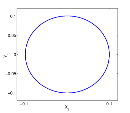
Figure 1: (a) Phase projections of System (5) with $o_{1}$=1, $o_{2}$=1.5, $o_{3}$=0.5, $o_{4}$=0.8, $Y_{2}$=1.

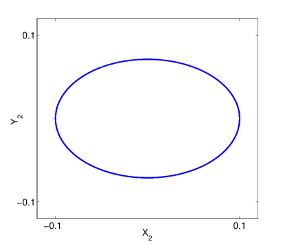
Figure 2: (b) The same as 1(a) but $Y_{1}$=1.

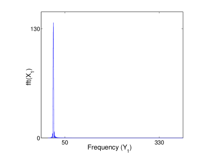
Figure 3: (a) Power spectra for the solutions of System (5) which correspond with 1(a).

Figure 4: (b) Power spectra for the solutions of System (5) which correspond with 1(b).

From Figs. 1, we can see the closed curves, which can be used to represent the phase projections of System (5). Based on the power spectra in Figs. 2, periodicity of Eqs. (1) is verified owing to the single frequency in Figs. 2. Thus, owing to the conclusions in Refs. dynamic1 ; dynamic2 , we know that System (5) is integrable, and Eqs. (1) do not admit any chaotic motions. Hereby, $fft(X_{1})$ and $fft(X_{2})$ represent the fast Fourier transform (FFT) of $X_{1}$ and $X_{2}$, respectively fft .

System (5) can be rewritten as

$$\left(\begin{array}[]{c}X_{1}\\ X_{2}\\ Y_{1}\\ Y_{2}\end{array}\right)_{\xi}=\left(\begin{array}[]{c}Y_{1}\\ Y_{2}\\ o_{1}X_{1}-o_{2}X_{1}^{3}-o_{2}X_{2}^{2}X_{1}\\ o_{3}X_{2}-o_{4}X_{2}^{3}-o_{4}X_{1}^{2}X_{2}\end{array}\right),$$ (14)

with $\mathbf{x_{1}}=(0,0,0,0)^{{}^{\prime}}$, $\mathbf{x_{2}}=\left(\pm\sqrt{\frac{o_{1}}{o_{2}}},0,0,0\right)^{{}^{\prime}}$ and $\mathbf{x_{3}}=\left(0,\pm\sqrt{\frac{o_{3}}{o_{4}}},0,0\right)^{{}^{\prime}}$ being its equilibrium points, where ^′ denotes the vector transpose. Without loss of generality, we choose $o_{1}$ and $o_{3}$ as the control parameters.

According to the time-delay feedback method chaotification1 ; chaotification2 , chaotifying System (5) is equivalent to to construct a single-input single-output system as follows:

$$\left\{\begin{array}[]{l}\vspace{1.5mm}\mathbf{x}_{\xi}=\mathbf{f}(\mathbf{x})+\mathbf{g}(\mathbf{x})\delta(\xi),\\ \vspace{1.5mm}y=h(\mathbf{x}),\end{array}\right.$$ (15)

where $\mathbf{x}$ and $y$ label the input and output, respectively, $\textbf{x}_{\xi}=d\textbf{x}/d\xi$, $\mathbf{f}(\mathbf{x})$ and $\mathbf{g}(\mathbf{x})$ are both real vector functions, $\delta(\xi)$ corresponds to a system parameter perturbation or an exogenous control input, and $h(\mathbf{x})$ is a smooth real function and refers to the output chaotification1 ; chaotification2 . Hereby, in the case of System (14), $\mathbf{x}=(X_{1},X_{2},Y_{1},Y_{2})^{{}^{\prime}}$, while $\mathbf{f}(\mathbf{x})$ and $\mathbf{g}(\mathbf{x})$ can be given as

$$\mathbf{f}(\mathbf{x})=\left(\begin{array}[]{c}Y_{1}\\ Y_{2}\\ o_{1}X_{1}-o_{2}X_{1}^{3}-o_{2}X_{2}^{2}X_{1}\\ o_{3}X_{2}-o_{4}X_{2}^{3}-o_{4}X_{1}^{2}X_{2}\end{array}\right),\ \ \ \mathbf{g}(\mathbf{x})=\left(\begin{array}[]{c}0\\ 0\\ X_{1}\\ X_{2}\end{array}\right).$$ (24)

Then, System (15) can be embodied as

$$\left\{\begin{array}[]{l}\vspace{1.5mm}\mathbf{x}_{\xi}=\left(\begin{array}[]{c}Y_{1}\\ Y_{2}\\ o_{1}X_{1}-o_{2}X_{1}^{3}-o_{2}X_{2}^{2}X_{1}\\ o_{3}X_{2}-o_{4}X_{2}^{3}-o_{4}X_{1}^{2}X_{2}\end{array}\right)+\left(\begin{array}[]{c}0\\ 0\\ X_{1}\\ X_{2}\end{array}\right)\delta(\xi),\\ \vspace{1.5mm}y=h(\mathbf{x}),\end{array}\right.$$ (25)

where $h(\mathbf{x})$ and $\delta(\xi)$ are to be determined.

Based on Expression (24), we have

$$\mathbf{ad_{f}g}(\mathbf{x})=\left(\begin{array}[]{c}-X_{1}\\ -X_{2}\\ Y_{1}\\ Y_{2}\end{array}\right),\ \ \ \mathbf{ad_{f}}^{2}\mathbf{g}(\mathbf{x})=\left(\begin{array}[]{c}-2Y_{1}\\ -2Y_{2}\\ 2o_{1}X_{1}-4o_{2}X_{1}^{3}+(2o_{1}-2o_{2})X_{1}X_{2}^{2}\\ 2o_{3}X_{2}-4o_{4}X_{2}^{3}+(2o_{3}-2o_{4})X_{2}X_{1}^{2}\end{array}\right),$$ (34)

$$\mathbf{ad_{f}}^{3}\mathbf{g}(\mathbf{x})=\left(\begin{array}[]{c}-4o_{1}X_{1}+6o_{2}X_{1}^{3}+(4o_{2}-2o_{1})X_{1}X_{2}^{2}\\ -4o_{3}X_{x}+6o_{4}X_{2}^{3}+(4o_{4}-2o_{3})X_{2}X_{1}^{2}\\ Y_{1}[4o_{1}-18o_{2}X_{1}^{2}+(2o_{1}-4o_{2})X_{2}^{2}]+(4o_{1}-8o_{2})X_{1}X_{2}Y_{2}\\ Y_{1}[4o_{3}-18o_{4}X_{2}^{2}+(2o_{3}-4o_{4})X_{1}^{2}]+(4o_{3}-8o_{4})X_{1}X_{2}Y_{1}\end{array}\right),$$ (39)

where $\textbf{ad}_{\textbf{f}}\textbf{g}(\textbf{x})$ refers to the Lie bracket chaotification1 ; chaotification2 of the two smooth vector functions $\mathbf{f}(\mathbf{x})$ and $\mathbf{g}(\mathbf{x})$. Note that the relative degree of System (25) is four, i.e., the dimension of $\mathbf{x}$, and the definition of “relative degree” can be seen in Refs. chaotification1 ; chaotification2 .

Via the conclusions in Refs. chaotification1 ; chaotification2 , $h(\mathbf{x})$ should satisfy

$$\frac{\partial h(\mathbf{x})}{\partial\mathbf{x}}[\mathbf{g}(\mathbf{x}),\mathbf{ad_{f}g}(\mathbf{x}),\mathbf{ad_{f}}^{2}\mathbf{g}(\mathbf{x})]=0.$$

Based on some calculations, it means that $h(\mathbf{x})$ can be expressed as

$$h(\mathbf{x})=X_{2}Y_{1}-X_{1}Y_{2},$$ (40)

which gives rise to the expressions of $\delta(\xi)$ as follows:

$$\delta(\xi)=\varsigma\sin[\sigma(X_{2}(\xi-\tau)Y_{1}(\xi-\tau)-X_{1}(\xi-\tau)Y_{2}(\xi-\tau))],$$ (41)

where $\varsigma$ and $\sigma$ are both the real constants, $\tau$ refers to the time-delay, and $\xi$ is given in Sec. 2.

Therefore, based on the chaotification of Eqs. (1), we can propose a chaotic system as follows:

$$\left(\begin{array}[]{c}X_{1}\\ X_{2}\\ Y_{1}\\ Y_{2}\end{array}\right)_{\xi}=\left(\begin{array}[]{c}Y_{1}\\ Y_{2}\\ (o_{1}+\delta)X_{1}-o_{2}X_{1}^{3}-o_{2}X_{2}^{2}X_{1}\\ (o_{3}+\delta)X_{2}-o_{4}X_{2}^{3}-o_{4}X_{1}^{2}X_{2}\end{array}\right),$$ (50)

where $\delta=\delta(\xi)=\varsigma\sin[\sigma(X_{2}(\xi-\tau)Y_{1}(\xi-\tau)-X_{1}(\xi-\tau)Y_{2}(\xi-\tau))]$ can be used as the perturbations of the control parameters $o_{1}$ and $o_{3}$.

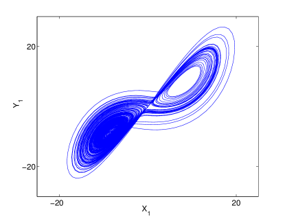
Figure 5: (a) Phase projection of $Y_{1}$ in System (50) with $Y_{2}$=1, $o_{1}$=1.5, $o_{2}$=0.2, $o_{3}$=1, $o_{4}$=2, $\varsigma$=1, $\sigma$=0.5 and $\tau$=10.

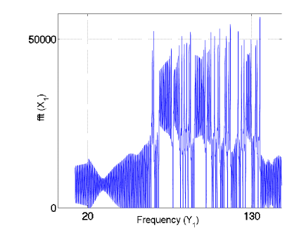
Figure 6: (b) Power spectra for $Y_{1}$ in System (50) which correspond with Fig. 3(a).

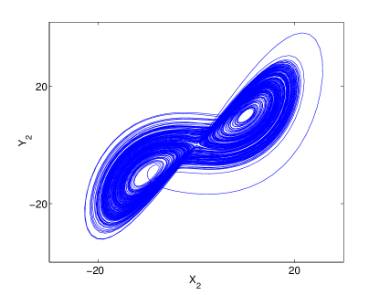
Figure 7: (a) Phase projection of $Y_{2}$ in System (50) with $Y_{1}$=1, $o_{1}$=1.5, $o_{2}$=0.2, $o_{3}$=1, $o_{4}$=2, $\varsigma$=1, $\sigma$=0.5 and $\tau$=10.

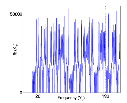
Figure 8: (b) Power spectra for $Y_{2}$ in System (50) which correspond with Fig. 4(a).

To study the final chaotic states of System (50), we investigate the phase projections of $Y_{1}$ and $Y_{2}$ in Figs. 3(a) and 4(a), respectively, and calculate their respective power spectra in Figs. 3(b) and 4(b). Comparing Figs. 3(b) with 2(a), 4(b) with 2(b), respectively, we can see that the original frequencies have been both broken, and chaotic motions occur. Note that the solutions of System (50) ignore the driver periods and represent a random sequence of uncorrelated shocks, so those chaotic motions are the “developed” ones developed1 ; developed2 .

In this paper, we have discussed the CNLS equations [i.e., Eqs. (1)], which describe the propagation of envelopes of electromagnetic waves in birefringent optical fibers, for their potential applications in the secured optical communication. With the time-delay and perturbations introduced into Eqs. (1), we have constructed a chaotic system and its final chaotic motions, with the phase projections and power spectra given. Further, soliton solutions and soliton propagation of such chaotic system have been studied when time-delay is fixed. As a generalization, the main results of this paper can be summarized as follows:

$\bullet$ Reducing Eqs. (1) into the equivalent four-dimensional planar dynamic system [i.e., System (5)], we have obtained the integrability and periodicity of Eqs. (1) from the phase projections and power spectra, as displayed in Figs. 1-2.

$\bullet$ With time-delay and perturbations into System (5), we have chaotified Eqs. (1) and a chaotic system [i.e., System 50] has been constructed.

$\bullet$ Chaotic motions of System (50) have been displayed via the phase projections, as shown in Figs. 3(a) and 4(a), and the respective power spectra have been calculated in Figs.3(b) and 4(b).

Acknowledgments The authors acknowledge *** for the discussions during the works.

References

- (1) A. Biswas, M. Fessak, S. Johnson, S. Beatrice, D. Milovic, Z. Jovanoski, R. Kohl and F. Majid, Opt. Laser Technol. 44, 263 (2012); D. Y. Tang, B. Zhao, D. Y. Shen, C. Lu, W. S. Man and H. Y. Tam,Phys. Rev. A 66, 033806 (2002).
- (2) D. Rand, I. Glesk, C. S. Bres, D. A. Nolan, X. Chen, J. Koh, J. W. Fleischer, K. Steiglitz and P. R. Prucnal,Phys. Rev. Lett. 98, 053902 (2007); Q. Tian, L. Wu, J. F. Zhang, B. A. Malomed, D. Mihalache and W. M. Liu,Phys. Rev. E 83, 016602 (2011).
- (3) M. I. Weinstein, SIAM J. Math. Anal. 16, 472 (1985); T. Ueda and W. L. Kath, Phys. Rev. A 42, 563 (1990).
- (4) T. Kanna, M. Lakshmanan, P. Tchofo Dinda, and Nail Akhmediev, Phys. Rev. E 73, 026604 (2006).
- (5) B. Tian, Y. T. Gao, Phys. Lett. A 342, 228 (2005); B. Tian, Y. T. Gao, Phys. Lett. A 359, 241 (2006).
- (6) Z. Y. Sun, Y. T. Gao, X. Yu, W. J. Liu and Y. Liu, Phys. Rev. E 80, 066608 (2009); A. Tonello, M. Szpulak, J. Olszewski, S. Wabnitz, A. B. Aceves and W. Urbanczyk, Opt. Lett. 34, 920 (2009); Q. L. Li, A. X. Zhang and X. F. Hua, Opt. Commun. 285, 118 (2012).
- (7) R. Radhakrishnan, M. Lakshmanan and J. Hietarinta,Phys. Rev. E 56, 2213 (1997); T. Kanna and M. Lakshmanan, Phys. Rev. Lett. 86, 5043 (2001); M. Vijayajayanthi, T. Kanna and M. Lakshmanan, Phys. Rev. A 77, 013820 (2008).
- (8) J. N. Lu, X. Q. Wu and J. H. Lü, Phys. Lett. A 305, 365 (2002).
- (9) Arman Kiani-B, Kia Fallahi, Naser Pariz and Henry Leung, Commun. Nonl. Sci. Numer. Simulat. 14, 863 (2009).
- (10) G. Kolumban, M. P. Kennedy and LO. Chua, IEEE Trans. Circ. Syst. 44, 927 (1997).
- (11) G. Heidari-Bateni and C. D. McGillem, IEEE Trans. Commun. 42, 154 (1994).
- (12) M. Lakshmanan and K. Murali, Chaos in Nonlinear Oscillators: Controlling and Synchronization (World Scientific, Singaopore, 1996).
- (13) T. Zhao, G. R. Chen and Q. Yang, Chaos 14, 662 (2004); X. S. Yang and Y. Tang, Chaos Solitons Fract. 19, 841 (2004); X. F. Wang, G. R. Chen and K. F. Man, IEEE Trans. Circ. Syst. 48, 641 (2001b); X. F. Wang, G. R. Chen and X. Yu, Chaos 10, 771 (2000).
- (14) G. D. Bergland, IEEE Spectrum 6, 228 (1969); P. Stoica and R. L. Moses, Introduction to Spectral Analysis (Prentice Hall, New Jersey, 1997).
- (15) M. C. Mackey and L. Class, Science 197, 287 (1977); J. D. Farmer, Physica D 4, 336 (1982); K. Ikeda and K. Matsumoto, Physica D 29, 223 (1987).
- (16) O. Diekmann, S. A. Gils, S. M. Lunel and H. O. Walther, Delay Equations: Funtional, Complex, and Nonlinear Analysis (Springer, Berlin, 1995).
- (17) H. Nijmeijer and A. Schaft, Nonlinear Dynamical Control Systems (Springer, New York, 1990); A. Isidori, Nonlinear Control Systems (Springer, Berlin, 1995); A. Isidori, Nonlinear Control Systems II (Springer, Berlin, 1999).
- (18) I. S. Amiria, A. Afroozeh, I. N. Nawi, M. A. Jalil, A. Mohamad, J. Ali and P. P. Yupapind, Procedia Engineering, 8, 417 (2011).
- (19) I. S. Amiria, A. Afroozeh, I. N. Nawi, M. A. Jalil, A. Mohamad, J. Ali and P. P. Yupapind, Procedia Engineering, 8, 360 (2011).
- (20) J. Yu, W. J. Zhang and X. M. Gao, Chaos Solitons Fract. 33, 1307 (2007).
- (21) E. Infeld and G. Rolands, Nonlinear Waves, Soliton and Chaos (Cambridge Univ., Cambridge, 1990).
- (22) H. J. Cao, J. M. Seoane and A. F. Sanjuán, Chaos Soliton. Fract. 34, 197 (2007).
- (23) B. Knobnob, S. Mitatha, K. Dejhan, S. Chaiyasoonthorn and P. P. Yupapin, Optick 121, 1743 (2010).
- (24) N. M. Ryskin and V. N. Titov, Tech. Phys. 48, 1170 (2011).
- (25) C. C. Lalescu, C. Meneveau and G. L. Eyink, Phys. Rev. Lett. 110, 084102 (2013).