Universality and quasicritical exponents of one-dimensional models displaying a quasitransition at finite temperatures

Abstract

Quasicritical exponents of one-dimensional models displaying a quasitransition at finite temperatures are examined in detail. The quasitransition is characterized by intense sharp peaks in physical quantities such as specific heat and magnetic susceptibility, which are reminiscent of divergences accompanying a continuous (second-order) phase transition. The question whether these robust finite peaks follow some power law around the quasicritical temperature is addressed. Although there is no actual divergence of these quantities at a quasicritical temperature, a power-law behavior fits precisely both ascending as well as descending part of the peaks in the vicinity but not too close to a quasicritical temperature. The specific values of the quasicritical exponents are rigorously calculated for a class of one-dimensional models (e.g. Ising-XYZ diamond chain, coupled spin-electron double-tetrahedral chain, Ising-XXZ two-leg ladder, and Ising-XXZ three-leg tube), whereas the same set of quasicritical exponents implies a certain “universality” of quasitransitions of one-dimensional models. Specifically, the values of the quasicritical exponents for one-dimensional models are: $\alpha=\alpha^{\prime}=3$ for the specific heat, $\gamma=\gamma^{\prime}=3$ for the susceptibility and $\nu=\nu^{\prime}=1$ for the correlation length.

I Introduction

Most one-dimensional systems in thermal equilibrium do not undergo a phase-transition at finite temperatures. Several arguments have been put forward giving support to the above statement as, for example, the one based on the entropic contribution of domain walls by Landau and Lifshitz landau , the Perron-Frobenius theorem for the non-degeneracy of the largest eigenvalue of a positive finite transfer matrix perron , and the van Hove’s theorem stating that the largest eigenvalue of a one-dimensional transfer matrix is an analytic function hove . A true phase-transition in one-dimensional equilibrium systems may develop either when the model system depicts long-range interactions or when a given interaction strength or a local degree of freedom diverges kittel ; weeks ; dauxois . Recently, Sarkanych et al. sarkanych proposed an interesting one-dimensional Potts model with "invisible states" and short-range coupling. By term invisible, they refer to an additional energy degeneracy, which contributes to the entropy, but not the interaction energy.

In addition, Cuesta and Sanchez cuesta summarized van Hove’s theorem is valid only under the following conditions: (i) the system must be homogeneous, excluding automatically inhomogeneous systems, i.e., disordered or aperiodic systems; (ii) the Hamiltonian does not include particles position terms, such as, external fields; (iii) the system must be considered as hard-core particles, while point-like or soft particles may be excluded. Then, Cuesta and Sanchez cuesta generalized the non-existence theorem of phase transition at finite temperatures. The extended theorem takes into account an external field and point-like particles, which broadens the Van Hove’s theorem, although this is not yet a fully general theorem. For example, this theorem cannot be applied for mixed particle chains or when more general external fields are considered.

Recent exact calculations for a few paradigmatic models bear evidence of remarkable "quasitransitions" of one-dimensional lattice-statistical systems with short-range and non-singular interactions gal15 ; tor16 ; roj16 ; str16 . In 2011 Timonin Timonin introduced the terms "pseudo-transitions" and "quasi-phases" by investigating the Ising spin ice in a magnetic field when referring to a sudden change in the first derivative and a sharp peak in the second derivative of the free energy although there are neither true discontinuities nor divergences in the appropriate derivatives of the free energy. Although the physical property observed by Timonin is precisely the same phenomenology presented by the models we study, here we use just for convenience the term "quasi" instead of "pseudo". The quasitransitions are thus reminiscent of discontinuous (first-order) phase transitions due to abrupt temperature-driven changes of entropy, internal energy and/or magnetization though these quantities display close to a quasicritical temperature steep but continuous variations instead of real discontinuities owing to analyticity of the free energy sou17 . On the other hand, the quasitransitions of one-dimensional lattice-statistical models are also reminiscent of continuous (second-order) phase transitions due to massive rise of the correlation length, specific heat and susceptibility in a vicinity of the quasicritical temperature though these quantities exhibit very sharp and robust finite-size peaks instead of actual divergences sou17 . The question whether these sizable peaks follow some power-law behavior near the quasicritical temperature is therefore quite intriguing and will be the main subject matter of the present work. It will be verified that these physical quantities indeed follow sufficiently close but not too close to a quasicritical temperature power laws. In addition, it will be demonstrated that the power-law behavior of seemingly diverse one-dimensional lattice-statistical models can be described by a unique set of “quasicritical” exponents, which enables us to conjecture the universality of “quasitransitions” of one-dimensional models.

A further investigation of quasitransitions and quasi-phases of one-dimensional spin systems was considered in Ref. Isaac , where the correlation function around the quasitransition temperature was discussed. The origin of quasitransition is however still not fully understood yet. The residual entropy at zero temperature has been shown to be a good indicator of the quasitransition as evidenced in Ref. org-psd .

It is demonstrated that the observed quasicritical behavior is a typical feature of a relatively wide class of one-dimensional Ising-Heisenberg spin models and in this respect, it might be therefore of experimental relevance for many real one-dimensional magnetic compounds of this type (see for instance references S-HW ; Heuvel-ch ; Bel-Oh ; Sahoo ; S-Honda ; Han-Strecka ; Torr-Jmmm , where Ising-Heisenberg models were applied to real compounds).

The present work is organized as follows. In Sec. 2 we will derive analytic expressions for quasicritical exponents of the correlation length, specific heat and magnetic susceptibility for one-dimensional lattice-statistical models, which can be rigorously mapped onto the effective Ising chain. In Sec. 3 we will specifically consider two particular cases from this class of exactly solved one-dimensional models: the spin-1/2 Ising-XYZ diamond chain and the coupled spin-electron double-tetrahedral chain. In Sec. 4 we will further verify the universality of quasicritical exponents by assuming another two exactly solved one-dimensional lattice-statistical models falling beyond this class of models: the spin-1/2 Ising-XXZ two-leg ladder and the spin-1/2 Ising-XXZ three-leg tube. Finally, our paper ends up with several concluding remarks and future outlooks.

II quasicritical exponents

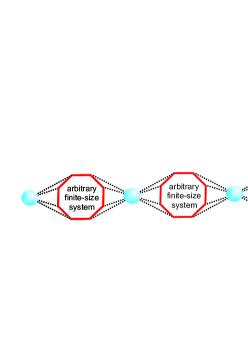
Figure 1: A schematic representation of decorated one-dimensional models, which consists of regularly alternating Ising spins (blue balls) and arbitrary finite-size lattice-statistical system (red octagons).

It is firmly established that several one-dimensional models, which can be viewed as the Ising chain decorated by arbitrary but finite lattice-statistical system (see Fig. 1 for a schematic representation), are exactly tractable by taking advantage of a generalized decoration-iteration transformation fis59 ; syo72 ; roj09 ; str10 ; strla ; roj11 . The decoration-iteration transformation furnishes a rigorous mapping correspondence between the decorated one-dimensional models and the effective Ising chain. This result would imply that the quasicritical exponents of the decorated models can be obtained from the generic Ising chain given by the effective Hamiltonian

$$H=-\sum_{i=1}^{N}\left[K_{0}+Ks_{i}s_{i+1}+\frac{h_{{\rm eff}}}{2}(s_{i}+s_{i+1})\right],$$ (1)

where $K_{0}$, $K$ and $h_{{\rm eff}}$ are effective temperature-dependent parameters unambiguously given by the ’self-consistency’ condition of the decoration-iteration transformation fis59 ; syo72 ; roj09 ; str10 ; strla ; roj11 . By imposing the periodic boundary condition the effective Ising chain can be readily solved by the transfer-matrix method, whereas the corresponding transfer matrix can be generally expressed as follows sou17

$$\mathbf{V}=\left(\begin{array}[]{cc}w_{1}&w_{0}\\ w_{0}&w_{-1}\end{array}\right).$$ (2)

The Boltzmann factors pertinent to each sector (i.e. transfer-matrix element) $n=\{-1,0,1\}$ are given by

$$w_{n}=\sum_{k=0}g_{n,k}{\rm e}^{-\beta\varepsilon_{n,k}},$$ (3)

where $\beta=1/(k_{B}T)$, $k_{B}$ is Boltzmann’s constant, $T$ is the absolute temperature, $\varepsilon_{n,k}$ labels the energy spectra for each sector $k=\{0,1,\ldots\}$ and $g_{n,k}$ denotes the respective degeneracy of each energy level. It follows from the transfer-matrix approach that the partition function can be expressed in terms of transfer-matrix eigenvalues $\mathcal{Z}_{N}=\lambda_{+}^{N}+\lambda_{-}^{N}$, which are explicitly given by

$$\lambda_{\pm}=\tfrac{1}{2}\Bigl{(}w_{1}+w_{-1}\pm\sqrt{(w_{1}-w_{-1})^{2}+4w_{0}^{2}}\Bigr{)}.$$ (4)

Then, the free energy attains in the thermodynamic limit ($N\rightarrow\infty$) the following simple expression

$$f=-\tfrac{1}{\beta}\ln\left[\tfrac{1}{2}\Bigl{(}w_{1}+w_{-1}+\sqrt{(w_{1}-w_{-1})^{2}+4w_{0}^{2}}\Bigr{)}\right].$$ (5)

Notice that all elements of the transfer matrix $\mathbf{V}$ are strictly positive, except at zero temperature. Therefore its eigenvalues are distinct and analytical according to Eq. (4), in agreement with the Perron-Frobenius theorem for matrices with all positive matrix elements. This implies in the absence of a true finite-temperature phase-transition in the one-dimensional Ising model.

A crossing of the transfer matrix eigenvalues would be required to achieve non-analiticity of the free-energy as it is expected in a phase-transition. It has been recently argued sou17 that a quasitransition may occur when the following condition is satisfied:

$$|w_{1}-w_{-1}|>w_{0}\gtrsim 0.$$ (6)

which can be reached at finite temperatures in a large class of effectively one-dimensional model systems. In what follows, we will unveil the leading behavior of some typical thermodynamic quantities under the above condition. For further convenience, it is therefore useful to define the small-size parameter $\bar{w}_{0}=\frac{w_{0}}{|w_{1}-w_{-1}|}\rightarrow 0$, which is suitable for Taylor series expansion. At first, let us consider the particular case when $w_{1}>w_{-1}$, then, the free energy (5) becomes

$$f= -\tfrac{1}{\beta}\ln\left[w_{1}+\tfrac{1}{2}\left(w_{1}-w_{-1}\right)\Bigl{(}\sqrt{1+4\bar{w}_{0}^{2}}-1\Bigr{)}\right],$$

$$= -\tfrac{1}{\beta}\ln(w_{1})-\tfrac{1}{\beta}\ln\left[1+\tfrac{\left(w_{1}-w_{-1}\right)(\sqrt{1+4\bar{w}_{0}^{2}}-1)}{2w_{1}}\right].$$ (7)

The last term of the second logarithm satisfies the following condition

$$0<\tfrac{\left(w_{1}-w_{-1}\right)(\sqrt{1+4\bar{w}_{0}^{2}}-1)}{2w_{1}}<1$$ (8)

and this condition guarantees convergence of the Taylor series expansion around $\bar{w}_{0}=0$. Hence, the first term will be more relevant than the higher-order contributions arising from the Taylor series expansion $\bar{w}_{0}\rightarrow 0$. Analogously, the similar expression can be obtained for the other particular case $w_{1}<w_{-1}$ by a mere inter-change of $w_{1}\leftrightarrow w_{-1}$. To summarize, the free energy (5) can be recast using the Taylor series expansion around $\bar{w}_{0}\rightarrow 0$ to the following form

$$f=\begin{cases}-\tfrac{1}{\beta}\ln(w_{1})-\tfrac{1}{\beta}\tfrac{w_{0}^{2}}{w_{1}\left(w_{1}-w_{-1}\right)}+\mathcal{O}(\bar{w}_{0}^{3}),&w_{1}>w_{-1}\\ -\tfrac{1}{\beta}\ln(\tilde{w}_{1}+\tilde{w}_{0}),&w_{1}=w_{-1}\\ -\tfrac{1}{\beta}\ln(w_{-1})-\tfrac{1}{\beta}\tfrac{w_{0}^{2}}{w_{-1}\left(w_{-1}-w_{1}\right)}+\mathcal{O}(\bar{w}_{0}^{3}),&w_{1}<w_{-1}\end{cases}$$ (9)

where $\tilde{w}_{1}=w_{1}=w_{-1}$, and $w_{0}=\tilde{w}_{0}$ under the specific condition $w_{1}=w_{-1}$. It is important to stress that the additional condition $|w_{1}-w_{-1}|\gg w_{0}$ must the fulfilled for the validity of the above asymptotic expansions when $w_{1}\neq w_{-1}$.

In order to characterize the power-law behavior emergent close to the quasitransition, it is useful to rewrite the Boltzmann factor in terms of the relative difference $\tau=\left(T_{p}-T\right)/T_{p}$ between temperature $T$ and quasicritical temperature $T_{p}$, defined as the temperature at which $w_{1}(T_{p})=w_{-1}(T_{p})$. To this end, one can use another Taylor series expansion of Boltzmann factors around $\beta\rightarrow\beta_{p}$, where $\beta-\beta_{p}=\frac{T_{p}-T}{T_{p}T}=\frac{1}{T}(1-\frac{T}{T_{p}})=\frac{\tau}{T}$. Thus, the Boltzmann’s factor can be expanded using Taylor series as a function of the inverse temperature $\beta$ around $\beta_{p}$, as follows

$$w_{n}(\beta)=w_{n}(\beta_{p})+\frac{\tau}{T_{p}}\frac{\partial w_{n}(\beta)}{\partial\beta}\Bigr{|}_{\beta=\beta_{p}}+\mathcal{O}\left(\tau^{2}\right).$$ (10)

Introducing the notation $w_{n}(\beta_{p})=\tilde{w}_{n}$ and $a_{n}\tilde{w}_{n}=\frac{\partial w_{n}(\beta)}{T_{p}\,\partial\beta}\Bigr{|}_{\beta=\beta_{p}}$ the above equation can be simplified to

$$w_{n}(\beta)= \tilde{w}_{n}+a_{n}\,\tilde{w}_{n}\tau+\mathcal{O}\left(\tau^{2}\right),$$

$$= \tilde{w}_{n}\left(1+a_{n}\tau\right)+\mathcal{O}\left(\tau^{2}\right),$$ (11)

Further, let us express the expression $w_{1}-w_{-1}$ entering into the denominator of Eq. (9) using this expansion

$$w_{1}-w_{-1}=\tilde{w}_{1}\left[a_{1}-a_{-1}\right]\tau+\mathcal{O}\left(\tau{}^{2}\right).$$ (12)

From this formula one readily attains the following relation

$$\left(a_{1}-a_{-1}\right)=\frac{1}{\tilde{w}_{1}T_{p}}\frac{\partial\left[w_{1}(\beta)-w_{-1}(\beta)\right]}{\partial\beta}\Bigr{|}_{\beta=\beta_{p}},$$ (13)

which is quite helpful for obtaining the coefficients of power laws pertinent to several physical quantities. An explicit formula for this parameter is given by Eq.  (46) in Appendix A. We emphasize that the development of power-law behavior is conditioned to Eq.(6) which implies that it is expected to hold when $\tau>\tilde{w}_{0}/(\tilde{w}_{1}|a_{1}-a_{-1}|)$. The condition $\tau\rightarrow 0$ implies that $\frac{\tilde{w}_{0}}{\tilde{w}_{1}|a_{1}-a_{-1}|}\rightarrow 0$, consequently, we must have $a_{1}\neq a_{-1}$. Therefore, it fails very close to the quasicritical temperature at which the thermodynamic functions are actually analytic.

II.1 Correlation length

The power-law behavior of the correlation length may be obtained analytically by manipulating the relation (13). First, let us rewrite $\frac{w_{1}}{w_{-1}}$ into the form

$$\frac{w_{1}}{w_{-1}}= 1+\left(a_{1}-a_{-1}\right)\tau+\mathcal{O}(\tau^{2}).$$ (14)

Furthermore, one gets the following expression by performing the logarithm of Eq. (14) in the limit of $\tau\rightarrow 0$

$$\ln\left(\tfrac{w_{1}}{w_{-1}}\right)= \ln\left[1+\left(a_{1}-a_{-1}\right)\tau\right]+\mathcal{O}(\tau^{2})$$

$$= \left(a_{1}-a_{-1}\right)\tau+\mathcal{O}(\tau^{2}).$$ (15)

The correlation length close to the quasitransition can be expressed as follows

$$\xi(\tau)=\left(\ln\tfrac{\lambda_{+}}{\lambda_{-}}\right)^{-1}=\begin{cases}\left(\ln\tfrac{w_{1}}{w_{-1}}\right)^{-1},&w_{1}>w_{-1}\\ \left(\ln\tfrac{w_{-1}}{w_{1}}\right)^{-1},&w_{1}<w_{-1}\end{cases}.$$ (16)

Using the leading-order term as given by Eq. (15), the correlation length (16) reduces in general to

$$\xi(\tau)=c_{{}_{\xi}}\;|\tau|^{-1}+\mathcal{O}(\tau^{0}),$$ (17)

where $c_{{}_{\xi}}=\frac{1}{|a_{1}-a_{-1}|}$ is constant independent of temperature. Consequently, around the quasicritical temperature, the correlation length generally follows the power-law function

$$\xi(\tau)\propto|\tau|{}^{-\nu},$$ (18)

whereas the relevant quasicritical exponent becomes $\nu=1$. We recall that this result fails very near the quasicritical point at which the correlation length remains finite. However, there may have a finite range of temperatures in the close vicinity of the quasicritical point on which a clear power-law behavior may develop, as we will illustrate in the forthcoming sections.

II.2 Specific heat

Another physical quantity of interest is the specific heat and its quasicritical exponents $\alpha$. To determine the quasicritical behavior of the specific heat, let us at first rewrite the free energy (7) for $w_{1}>w_{-1}$, and using the relation (12) in the following form

$$f=-T_{p}(1-\tau)\ln(1+a_{1}\tau)-\frac{T_{p}(1-\tau)\tilde{w}_{0}^{2}(1+a_{0}\tau)^{2}}{\tilde{w}_{1}^{2}(1+a_{1}\tau)(a_{1}-a_{-1})\tau}.$$ (19)

By considering only the leading-order term from the Taylor series expansion, the free energy reduces to

$$f= -\left(\frac{\tilde{w}_{0}}{\tilde{w}_{1}}\right)^{2}\frac{T_{p}}{(a_{1}-a_{-1})}\tau^{-1}+{\cal O}(\tau^{0})$$ (20)

$$\approx -c_{{}_{f}}\,\tau^{-1},$$ (21)

where $c_{{}_{f}}=\left(\frac{\tilde{w}_{0}}{\tilde{w}_{1}}\right)^{2}\frac{T_{p}}{(a_{1}-a_{-1})}$ is a constant independent of temperature. For $w_{1}<w_{-1}$, we have a very similar expression $c_{{}_{f}}=\left(\frac{\tilde{w}_{0}}{\tilde{w}_{1}}\right)^{2}\frac{T_{p}}{(a_{-1}-a_{1})}$.

Now, one may perform a derivative of the free energy with respect to temperature. In doing so, one gets the following expression for the entropy as a function of the temperature

$$\mathcal{S}(\tau)= -\left(\frac{\partial f}{\partial\tau}\right)\left(\frac{\partial\tau}{\partial T}\right)=-c_{{}_{f}}\,\tau^{-2}\left(\frac{-1}{T_{p}}\right)$$

$$= \frac{c_{{}_{f}}}{T_{p}}\,\tau^{-2}.$$ (22)

The above equation can be straightforwardly used in order to obtain the formula governing temperature variations of the specific heat in a vicinity of the quasicritical temperature

$$C(\tau)=T\left(\frac{\partial\mathcal{S}}{\partial\tau}\right)\left(\frac{\partial\tau}{\partial T}\right)=2\frac{c_{{}_{f}}}{T_{p}}\,\tau^{-3}.$$ (23)

It is obvious from Eq. (23) that, around the quasicritical temperature, the specific heat follows the power law

$$C(\tau)\propto|\tau|{}^{-\alpha},$$ (24)

whereas the relevant quasicritical exponent is $\alpha=3$. Again, this singularity becomes rounded as one ultimately approaches the quasicritical temperature.

II.3 Magnetic Susceptibility

Last but not least, let us explore the power-law behavior of the magnetic susceptibility around the quasicritical temperature. For this aim, we will at first derive the explicit formula for the magnetization

$$M(\tau,h)=- \left(\frac{\partial f}{\partial\tau}\right)\left(\frac{\partial\tau}{\partial h}\right)=-c_{{}_{f}}\,\left(\frac{\partial\tau}{\partial h}\Bigr{|}_{h_{p},T_{p}}\right)\tau^{-2}.$$ (25)

It is important to note that the parameters $T_{p}$ and $h_{p}$ are constrained by the relation $w_{1}(T_{p},h_{p})=w_{-1}(T_{p},h_{p})$, which was denoted merely as $\tilde{w}_{1}=\tilde{w}_{-1}$. The isothermal susceptibility is determined in the vicinity of the quasicritical temperature just by the lowest-order term from the Taylor series expansion

$$\chi(\tau,h)= \left(\frac{\partial M}{\partial\tau}\right)\frac{\partial\tau}{\partial h}=2c_{{}_{f}}\,\left(\frac{\partial\tau}{\partial h}\Bigr{|}_{h_{p},T_{p}}\right)^{2}\tau^{-3},$$ (26)

where

$$\frac{\partial\tau}{\partial h}\Bigr{|}_{h_{p},T_{p}}=\frac{w_{1,h_{p}}-w_{-1,h_{p}}}{\tilde{w}_{1}\left(a_{1}-a_{-1}\right)},$$ (27)

with $w_{1,h_{p}}=\frac{\partial w_{1}}{\partial h}|_{h_{p}}$ and $w_{-1,h_{p}}=\frac{\partial w_{-1}}{\partial h}|_{h_{p}}$. The Eq.(27) is valid for both condition $w_{1}>w_{-1}$ or $w_{-1}>w_{1}$. Accordingly, the magnetic susceptibility follows the power law

$$\chi(\tau)\propto|\tau|{}^{-\gamma},$$ (28)

around the quasicritical temperature, whereas the relevant quasicritical exponent is $\gamma=3$. This power-law behavior ultimately rounds in the very close vicinity of the quasicritical temperature at which the magnetic susceptibility remains finite. Notice that the quasicritical temperature occurs for all physical observables at same point, the quasicritical temperature can be obtain using the condition $w_{1}(T_{p})=w_{-1}(T_{p})$.

III Applications

In this section, we will compare the quasicritical exponents as obtained in the previous section from the approximate Taylor series expansion performed around the quasicritical temperature with the relevant exact results for two paradigmatic exactly solved models shown in Fig. 2(a)-(b), which can be rigorously mapped onto the effective Ising chain. More specifically, we will comprehensively explore the quasitransition of the spin-1/2 Ising-XYZ diamond chain tor16 shown in Fig. 2(a) and the coupled spin-electron double-tetrahedral chain gal15 depicted in Fig. 2(b), respectively.

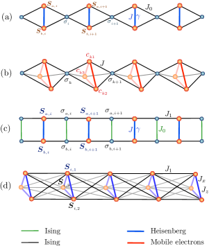
Figure 2: A schematic illustration of four considered one-dimensional models displaying a quasitransition: (a) Ising-XYZ diamond chain; (b) coupled spin-electron double-tetrahedral chain; (c) Ising-Heisenberg two-leg ladder; (d) Ising-Heisenberg three-leg tube. The former two models belong to a class of one-dimensional models shown in Fig. 1, which can be rigorously mapped onto the effective Ising chain. The latter two models do not belong to this class.

III.1 Ising-XYZ diamond chain

The spin-1/2 Ising-XYZ diamond chain has been introduced and exactly solved in Ref. lis14 , whereas its quasitransition has been discovered and detailed examined in Refs. tor16 ; sou17 . This model schematically shown in Fig. 2(a) assumes a regular alternation of the Ising spins $S_{i}=1/2$ with a couple of the Heisenberg spins described by the Pauli spin operators $\sigma_{a(b),i}^{\alpha}$ ($\alpha=\{x,y,z\}$), whereas the relevant Hamiltonian reads

$$H= -\sum_{i=1}^{N}\left[J(1+\gamma)\sigma_{a,i}^{x}\sigma_{b,i}^{x}+J(1-\gamma)\sigma_{a,i}^{y}\sigma_{b,i}^{y}+\right.$$

$$+J_{z}\sigma_{a,i}^{z}\sigma_{b,i}^{z}+J_{0}(\sigma_{a,i}^{z}+\sigma_{b,i}^{z})(S_{i}+S_{i+1})+$$

$$\left.+h_{0}(\sigma_{a,i}^{z}+\sigma_{b,i}^{z})+\frac{h}{2}(S_{i}+S_{i+1})\right].$$ (29)

Above, the parameter $J_{0}$ denotes the Ising exchange interaction between the nearest-neighbor Ising and Heisenberg spins, the XYZ exchange coupling between the nearest-neighbor Heisenberg spin pairs is given by three coupling constants: $J_{z}$ corresponding to the $z$-component, $J$ corresponding to the $xy$-component and $\gamma$ being the XY-anisotropy. Besides, the effect of external magnetic field $h$ ($h_{0}$) acting on the Heisenberg spins (Ising spins) is considered as well.

It turns out that the free energy (5) of this model can be expressed in terms of the relevant Boltzmann factors, which are given by the following relations (see Ref. sou17 for further details)

$$w_{n}=2{\rm e}^{\frac{\beta nh_{0}}{2}}\left[{\rm e}^{-\frac{\beta J_{z}}{4}}{\rm cosh}\left(\tfrac{\beta J}{2}\right)+{\rm e}^{\frac{\beta J_{z}}{4}}{\rm cosh}\left(\beta\Delta_{n}\right)\right].$$ (30)

with $\Delta_{n}=\sqrt{\left(h+J_{0}n\right)^{2}+\tfrac{1}{4}J^{2}\gamma^{2}}$ and $n=-1,0,1$.

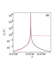
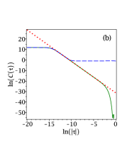
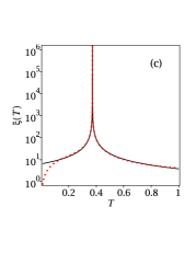
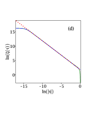
Figure 3: Temperature variations of the specific heat and correlation length of the spin-1/2 Ising-XYZ diamond chain (29) in a semi-logarithmic (left panel) and logarithmic (right panel) scale in a vicinity of the quasicritical temperature for the particular set of the interaction parameters: $J=100$, $J_{z}=24$, $J_{0}=-24$, $\gamma=0.7$ and $h=12.7$. Left panel: solid lines correspond to exact results, while dotted lines correspond to Taylor series expansion as given by Eqs. (23) and (17), respectively. Right panel: solid (dashed) lines correspond to exact results for $\tau<0$ ($\tau>0$), while dotted lines are the power-law functions $\ln(C(\tau))=-3\ln(|\tau|)-31.37$ and $\ln(\xi(\tau))=-\ln(|\tau|)+1.86$, respectively.

Typical temperature variations of the specific heat and correlation length of the spin-1/2 Ising-XYZ diamond chain are reported in Fig. 3 for the set of parameters $J=100$, $J_{z}=24$, $J_{0}=-24$, $\gamma=0.7$, and $h=12.7$, which are consistent with emergence of a quasitransition at the quasicritical temperature $T_{p}=0.37262119$. The readers interested in further details concerning the specific heat and correlation length are referred to Ref. sou17 . In Fig. 3(a) the specific heat $C(T)$ is plotted against temperature $T$, whereas a solid line represents exact results as given in Refs. tor16 ; sou17 and a dotted line denotes Taylor series expansion around the quasicritical temperature as given by Eq. (23). The temperature dependence of $\ln(C(\tau))$ versus $\ln(|\tau|)$ depicted in Fig. 3(b) verifies existence of intermediate temperature range, where the specific heat follows the power law (a straight line in log-log scale) with the critical exponent $\alpha=\alpha^{\prime}=3$. Exact results for the specific heat are indeed consistent with $\ln(C(\tau))=-3\ln(|\tau|)-31.37$ as obtained from Taylor series expansion given by Eq.(23). Furthermore, the correlation length $\xi(T)$ is displayed against $T$ in Fig. 3(c), where the relevant exact results are depicted by a solid line and the Taylor series expansion given by Eq. (17) by a dotted line. It can be seen from $\ln(\xi(\tau))$ vs. $\ln(|\tau|)$ dependence shown in Fig. 3(d) that the correlation length follows sufficiently close but not too close to a quasicritical temperature the power law with the critical exponent $\nu=\nu^{\prime}=1$. In fact, the exact results reported in Refs. tor16 ; sou17 are in reasonable accordance with the Taylor series expansion as given by Eq. (17) illustrated as a straight dotted line.

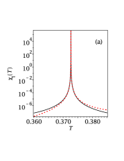
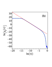
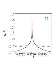
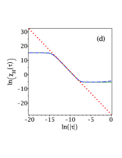
Figure 4: Temperature variations of the magnetic susceptibility of the Ising ($\chi_{I}$) and Heisenberg ($\chi_{H}$) spins for the spin-1/2 Ising-XYZ diamond chain (29). The same parameter set is used as in Fig.3. Left panel: solid lines correspond to exact results, while dotted lines correspond to Taylor series expansion as given by Eqs. (26). Right panel: solid (dashed) lines correspond to exact results for $\tau<0$ ($\tau>0$), while dotted lines are the power-law functions $\ln(\chi_{{}_{I}}(\tau))=-3\ln(|\tau|)-26.667$ and $\ln(\chi_{{}_{H}}(\tau))=-3\ln(|\tau|)-27.976$.

Last but not least, the magnetic susceptibility $\chi_{{}_{I}}(T)$ of the Ising spins is displayed in Fig. 4(a) as a function of temperature $T$, whereas a solid line refers to exact results derived in Refs. tor16 ; sou17 and a dotted line labels asymptotic expression as obtained from Taylor series expansion given by Eq. (26). The magnetic susceptibility shown in Fig. 4(b) in the form $\ln(\chi_{{}_{I}}(\tau))$ against $\ln(|\tau|)$ plot corroborates an intermediate temperature range, where the magnetic susceptibility follows the power law with the critical exponent $\gamma=\gamma^{\prime}=3$. The dotted line, which was obtained from Taylor series expansion given by Eq. (26) with the asymptotic form $\ln(\chi_{{}_{I}}(\tau))=-3\ln(|\tau|)-26.667$, is in this temperature range in a plausible agreement with the exact results. Similar findings hold for the magnetic susceptibility of the Heisenberg spin $\chi_{{}_{H}}(T)$, which is illustrated in Fig.4(c) and 4(d). However, it is worth noticing that the magnetic susceptibility of the Ising spins follows the relevant power-law function in a wider temperature region as compared to the magnetic susceptibility of the heisenberg spins.

It could be concluded that the specific heat, magnetic susceptibility and correlation length of the spin-1/2 Ising-XYZ diamond chain driven sufficiently close but not too close to a quasicritical temperature are characterized by the power-law functions with the critical exponents $\alpha=\alpha^{\prime}=3$, $\gamma=\gamma^{\prime}=3$ and $\nu=\nu^{\prime}=1$. Of course, this description inevitably breaks down at the quasicritical temperature as the system does not exhibit actual divergence of the relevant physical quantities.

III.2 Spin-electron double-tetrahedral chain

Next, let us consider a coupled spin-electron model on a double-tetrahedral chain schematically depicted in Fig. 2(b), in which one localized Ising spin situated at nodal site regularly alternates with a triangular plaquette composed of three decorating sites available to two mobile electrons. This one-dimensional spin-electron system has been introduced and exactly solved in Ref. gal15 , where the outstanding temperature dependencies of several physical quantities mimicking a phase transition were also reported. The coupled spin-electron model on a double-tetrahedral chain can be defined as a sum over block Hamiltonians ${\cal H}_{k}$

$${\cal H}=\sum_{k=1}^{N}{\cal H}_{k},$$ (31)

whereas each block Hamiltonian ${\cal H}_{k}$ involves all the interaction terms connected to two mobile electrons delocalized over the $k$th triangular plaquette

$${\cal H}_{k}\!\! = \!\!-t\sum_{\alpha=\uparrow,\downarrow}\!(c_{k1,\alpha}^{\dagger}c_{k2,\alpha}\!+c_{k2,\alpha}^{\dagger}c_{k3,\alpha}\!+c_{k3,\alpha}^{\dagger}c_{k1,\alpha}\!+{\rm h.c.})$$ (32)

$$+ \!\!\frac{J}{2}(\sigma_{k}^{z}+\sigma_{k+1}^{z})\sum_{j=1}^{3}\,(n_{kj,\uparrow}-n_{kj,\downarrow})+U\sum_{j=1}^{3}n_{kj,\uparrow}n_{kj,\downarrow}$$

$$- \!\!\frac{h_{{\rm I}}}{2}(\sigma_{k}^{z}+\sigma_{k+1}^{z})-\frac{h_{{\rm e}}}{2}\sum_{j=1}^{3}\,(n_{kj,\uparrow}-n_{kj,\downarrow}).$$

Here, $c_{kj,\alpha}^{\dagger}$ and $c_{kj,\alpha}$ label standard fermionic creation and annihilation operators for mobile electrons from the $k$th triangular plaquette with spin $\alpha$ = $\uparrow$ or $\downarrow$, $n_{kj,\alpha}=c_{kj,\alpha}^{\dagger}c_{kj,\alpha}$ is the respective number operator and $\sigma_{k}^{z}=\pm 1/2$ denotes the Ising spin situated at the $k$th nodal site. The hopping term $t>0$ accounts for the kinetic energy of mobile electrons delocalized over triangular plaquettes, the Coulomb term $U>0$ is energy penalty for two electrons with opposite spins situated at the same decorating site and the coupling constant $J$ determines the Ising-type nearest-neighbor interaction between the localized Ising spins and the mobile electrons. Finally, the Zeeman’s terms $h_{{\rm I}}$ and $h_{{\rm e}}$ account the magnetostatic energy of the localized Ising spins and mobile electrons in a static magnetic field.

A diagonalization of the block Hamiltonian (32) gives a full energy spectrum (see Eq. (5) in Ref. gal15 ), whereas the resulting expression for the relevant Boltzmann factor obtained from this complete set of eigenvalues reads

$$w_{n}= {\rm e}^{\beta\frac{n}{2}h_{{\rm I}}}\Big{\{}\!\!\left(\!2{\rm e}^{\beta t}+{\rm e}^{-2\beta t}\right)\!\left(1+2\cosh\left[\beta(Jn-h_{{\rm e}})\right]\right)$$

$$+\,4{\rm e}^{-\beta t/2-\beta U/2}\cosh\left[\frac{\beta}{2}\!\sqrt{(U\!-t)^{2}\!+8t^{2}}\,\right]$$

$$+\negmedspace 2{\rm e}^{\beta t-\beta U/2}\cosh\negmedspace\left[\frac{\beta}{2}\!\sqrt{(U\!+2t)^{2}\!+32t^{2}}\,\right]\negmedspace\Big{\}}$$ (33)

with the parameter $n=(\sigma_{k}^{z}+\sigma_{k+1}^{z})$ defined for the sake of brevity. The free energy for the coupled spin-electron double-tetrahedral chain can be consequently obtained from Eq. (5) by assuming $w_{-1}$, $w_{0}$ and $w_{1}$.

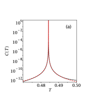
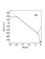
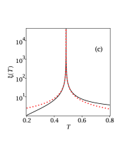
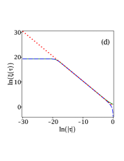
Figure 5: Temperature variations of the specific heat and correlation length of the coupled spin-electron double-tetrahedral chain (32) in a semi-logarithmic (left panel) and logarithmic (right panel) scale in a close vicinity of the quasitransition for the particular set of the interaction parameters $t=8.5$, $U=20$ and $J=20$. Left panel: solid lines correspond to exact results, while dotted lines correspond to Taylor series expansion as given by Eqs. (23) and (17), respectively. Right panel: solid (dashed) lines correspond to exact results for $\tau<0$ ($\tau>0$), while dotted lines are the power-law functions $\ln(C(\tau))=-3\ln(|\tau|)-38.86$ and $\ln(\xi(\tau))=-\ln(|\tau|)+0.366$, respectively.

It has been argued in Ref. gal15 that the coupled spin-electron double-tetrahedral chain given by the Hamiltonian (32) mimics a phase transition at the quasicritical temperature

$$T_{p}=\frac{\sqrt{(U+2t)^{2}+32t^{2}}-U-2J}{\ln 4}.$$ (34)

To illustrate the case, we depict in Fig. 5 typical temperature variations of the specific heat and correlation length by assuming the set of interaction parameters $t=8.5$, $U=20$, $J=20$ and $h_{e}=h_{I}=20$, which lead to a quasitransition at the quasicritical temperature $T_{p}=(\sqrt{3681}-60)/(\ln 4)\approx 0.4842011$. Fig. 5(a) compares exact results for temperature dependence of the specific heat $C(T)$ (solid line) derived according to Ref. gal15 with the asymptotic formula (23) derived from Taylor series expansion around the quasicritical temperature (dotted line). It turns out that the specific heat actually follows sufficiently close but not too close to the quasicritical temperature the power law with the critical exponent $\alpha=\alpha^{\prime}=3$ as it is evidenced by a straight dotted line $\ln(C(\tau))=-3\ln(|\tau|)-38.8592$ shown in Fig. 5(b) in the respective $\ln(C(\tau))$ vs. $\ln(|\tau|)$ dependence. Similarly, exact results for temperature dependence of the correlation length $\xi(T)$ (solid line) are plotted in Fig. 5(c) along with asymptotic expression (17) (dotted line) derived from the Taylor series expansion around the quasicritical temperature. It is quite evident from $\ln(\xi(\tau))$ vs. $\ln(|\tau|)$ dependence shown in Fig. 5(d) that the correlation length is governed the power law (17) with the quasicritical exponent $\nu=\nu^{\prime}=1$ if temperature is set sufficiently close but not too close to a quasicritical one.

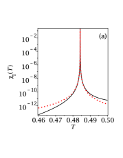
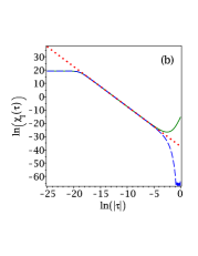
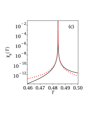
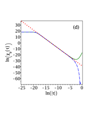
Figure 6: Temperature variations of the magnetic susceptibility of the Ising spins ($\chi_{I}$) and the mobile electrons ($\chi_{e}$) for the coupled spin-electron double-tetrahedral chain (32). The same parameter set is used as in Fig.5. Left panel: solid lines correspond to exact results, while dotted lines correspond to Taylor series expansion as given by Eqs. (26). Right panel: solid (dashed) lines correspond to exact results for $\tau<0$ ($\tau>0$), while dotted lines are the power-law functions $\ln(\chi_{{}_{I}}(\tau))=-3\ln(|\tau|)-38.40$ and $\ln(\chi_{e}(\tau))=-3\ln(|\tau|)-38.50$.

Finally, exact results (solid line) for temperature variations of the magnetic susceptibility of the Ising spins $\chi_{{}_{I}}(T)$ depicted in Fig. 6(a) are in plausible concordance with the asymptotic expression (26) obtained from Taylor series expansion around the quasicritical temperature. In addition, $\ln(\chi_{{}_{I}}(\tau))$ against $\ln(|\tau|)$ plot displayed in Fig. 6(b) verifies existence of an intermediate temperature region, where exact results for the susceptibility (solid line) follow the power law $\ln(\chi_{{}_{I}}(\tau))=-3\ln(|\tau|)-38.4009$ with the critical exponent $\gamma=\gamma^{\prime}=3$ (dotted line) obtained from Taylor series expansion (26). Analogously, the magnetic susceptibility of the mobile electrons is shown in Fig.6(c) and 6(d), where a similar coincidence is found with the power-law dependence characterized through almost the same constants $\ln(\chi_{e}(\tau))=-3\ln(|\tau|)-38.4995$.

To summarize, it has been found that the specific heat, magnetic susceptibility and correlation length of the coupled spin-electron double-tetrahedral chain are governed in a close vicinity of the quasicritical temperature by the power-law functions, which are characterized by the same set of quasicritical exponents $\alpha=\alpha^{\prime}=3$, $\gamma=\gamma^{\prime}=3$ and $\nu=\nu^{\prime}=1$ as reported previously for the spin-1/2 Ising-XYZ diamond chain even though both one-dimensional lattice-statistical models are very different in their nature.

IV ”quasicriticality” of other one-dimensional models

In this section, we will comprehensively explore the quasicritical exponents of other one-dimensional lattice-statistical models, which cannot be in principle mapped onto the effective Ising chain. It will be demonstrated hereafter that the quasicritical exponents of other paradigmatic examples of one-dimensional models displaying a quasitransition at finite temperatures will remain the same, which indicates a certain universality of the quasitransitions. More specifically, we will exactly validate quasicritical exponents of the spin-1/2 Ising-XXZ two-leg ladder roj16 and the spin-1/2 Ising-XXZ three-leg tube str16 , respectively.

IV.1 Ising-XXZ two-leg ladder

First, let us examine quasicritical exponents of the the spin-1/2 Ising-XXZ two-leg ladder with regularly alternating Ising and Heisenberg rungs as schematically represented in Fig. 2(c). The Hamiltonian of the investigated one-dimensional spin system can be expressed by

$$\mathcal{H}=\sum_{i=1}^{N}\left(H_{i}^{XXZ}+H_{i,i+1}^{I}+H_{i,i+1}^{IH}\right)$$ (35)

with

$$H_{i}^{XXZ}= -J_{x}(S_{a,i}^{x}S_{b,i}^{x}+S_{a,i}^{y}S_{b,i}^{y})-J_{z}S_{a,i}^{z}S_{b,i}^{z},$$

$$H_{i,i+1}^{I}= -\frac{J_{0}}{2}(\sigma_{a,i}\sigma_{b,i}+\sigma_{a,i+1}\sigma_{b,i+1}),$$

$$H_{i,i+1}^{IH}= -J_{1}(\sigma_{a,i}+\sigma_{a,i+1})S_{a,i}^{z}-J_{1}(\sigma_{b,i}+\sigma_{b,i+1})S_{b,i}^{z}.$$ (36)

Here, $S_{\gamma,i}^{\alpha}$ ($\alpha=\{x,y,z\}$) denote three spatial components of the spin-1/2 operator pertinent to two Heisenberg spins $\gamma=\{a,b\}$ from the $i$th rung and $\sigma_{\gamma,j}=\pm 1/2$ refer to two Ising spins $\gamma=\{a,b\}$ from the $j$th rung (see Fig. 2(c) for a schematic illustration). The exchange constants $J_{0}$ and $J_{1}$ label the Ising intra-rung and intra-leg interactions, while the XXZ Heisenberg intra-rung interaction is determined by its $xy$-component $J_{x}$ and $z$-component $J_{z}$.

It has been proved in Ref. roj16 that the spin-1/2 Ising-XXZ two-leg ladder can be rigorously mapped onto the mixed spin-3/2 and spin-1/2 Ising-Heisenberg diamond chain, which can be subsequently exactly solved within the transfer-matrix method. In a consequence of that, one can obtain the exact expression for the free energy of the spin-1/2 Ising-XXZ two-leg ladder (see Eq. (40) in Ref. roj16 ), which is formally identical with the formula (5) of the effective Ising chain depending on three different Boltzmann’s factors. Owing to this fact, the spin-1/2 Ising-XXZ two-leg ladder may display a similar quasitransition as the one-dimensional models studied in the previous section whenever the three effective Boltzmann’s factors satisfy the condition (6).

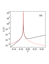
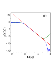
Figure 7: Temperature variations of the specific heat of the spin-$1/2$ Ising-XXZ two-leg ladder in a vicinity of the quasicritical temperature by assuming the following set of coupling constants $J_{0}=25$, $J_{x}=21.8$, $J_{z}=25$ and $J_{1}=-30$: (a) exact results (solid line) for $C$ versus $T$ dependence is compared to the power-law function (dotted line); (b) exact results for $\ln(C(\tau))-\ln(|\tau|)$ dependence above (below) the quasicritical temperature $\tau<0$ ($\tau>0$) shown as a solid (dashed) line are compared to the power-law function $\ln(C(\tau))=-3\ln(|\tau|)-22.2$ depicted by a dotted line.

To support this statement, the specific heat of the spin-1/2 Ising-XXZ two-leg ladder is displayed in Fig. 7(a) a function of temperature for the fixed values of the interaction constants $J_{0}=25$, $J_{x}=21.8$, $J_{z}=25$ and $J_{1}=-30$ being responsible for a quasitransition at the quasicritical temperature $T_{p}=0.186778$. The solid line corresponds to the exact results derived according to Ref. roj16 , while the dotted line denotes the relevant power-law function. Temperature variations of the specific heat, which are shown in Fig. 7(b) in the form of $\ln(C(\tau))$ versus $\ln(|\tau|)$ plot, bear evidence that the massive rise of the specific heat sufficiently close but not too close to the quasicritical temperature is driven by the power-law function $\ln(C(\tau))=-3\ln(|\tau|)-22.2$ being consistent with the quasicritical exponents $\alpha=\alpha^{\prime}=3$. From this perspective, the critical exponents of the spin-1/2 Ising-XXZ two-leg ladder belong to the same universality class as reported previously for the one-dimensional lattice-statistical models, which can be rigorously mapped onto the effective Ising chain.

IV.2 Ising-XXZ three-leg tube

Second, we will also investigate a quasitransition of the spin-$1/2$ Ising-XXZ three-leg tube str16 shown in Fig. 2(d), which takes into account the XXZ intra-triangle interaction between the spins from the same triangular unit and the Ising inter-triangle interaction between the spins from neighboring triangular units. The Hamiltonian of the spin-$1/2$ Ising-XXZ three-leg tube is defined as

$${H}\!\!\! = \!\!\!\sum_{i=1}^{N}\sum_{j=1}^{3}\left[J_{x}\left({S}_{i,j}^{x}{S}_{i,j+1}^{x}+{S}_{i,j}^{y}{S}_{i,j+1}^{y}\right)+J_{z}{S}_{i,j}^{z}{S}_{i,j+1}^{z}\right]$$ (37)

$$+ \!\!\!J_{1}\sum_{i=1}^{N}\left(\sum_{j=1}^{3}{S}_{i,j}^{z}\right)\left(\sum_{j=1}^{3}{S}_{i+1,j}^{z}\right),$$

where ${S}_{i,j}^{\alpha}$ $(\alpha\in\{x,y,z\})$ denote three spacial components of the spin-$1/2$ operator, the first subscript $i$ specifies a triangular unit in the three-leg tube and the second subscript $j$ determines a position of individual spin in a given triangular unit. The coupling constants $J_{x}$ and $J_{z}$ denote the XXZ intra-triangle interaction between the spins belonging to the same triangular unit, while the other interaction term $J_{1}$ refers to the Ising inter-triangle interaction between the spins from neighboring triangular units.

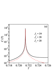
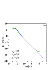
Figure 8: Temperature variations of the specific heat of the spin-$1/2$ Ising-XXZ three-leg tube in a vicinity of the quasicritical temperature by assuming the following set of coupling constants $J_{1}=20$, $J_{z}=20$ and $J_{x}=39$: (a) exact results (solid line) for $C$ versus $T$ dependence is compared to the power-law function (dotted line); (b) exact results for $\ln(C(\tau))-\ln(|\tau|)$ dependence above (below) the quasicritical temperature $\tau<0$ ($\tau>0$) shown as a solid (dashed) line are compared to the power-law function $\ln(C(\tau))=-3\ln(|\tau|)-31.7$ depicted by a dotted line.

It is worthwhile to remark that the spin-$1/2$ Ising-XXZ three-leg tube is fully quantum one-dimensional model because each spin of the three-leg tube is involved in two XXZ exchange interactions and six Ising interactions. In spite of this fact, the spin-$1/2$ Ising-XXZ three-leg tube is still exactly solvable within the classical transfer-matrix method because the total spin on a triangular unit represents locally conserved quantity with well defined quantum spin numbers str16 . The free energy and full thermodynamics of the spin-$1/2$ Ising-XXZ three-leg tube has been reported in our previous work str16 to which the readers interested in further details are referred to. It is nevertheless worth noticing that the exact result for the free energy of the spin-$1/2$ Ising-XXZ three-leg tube given by Eq. (12) of Ref. str16 has similar structure as the formula (5) of the effective Ising chain depending on three different Boltzmann’s factors.

In what follows, our attention will be limited to a detailed analysis of a quasitransition of the spin-$1/2$ Ising-XXZ three-leg tube, which is emergent at the following quasicritical temperature str16

$$T_{p}=\frac{4J_{1}-2J_{z}-J_{x}}{\ln 4}.$$ (38)

For illustration, typical temperature variations of the specific heat of the spin-$1/2$ Ising-XXZ three-leg tube are depicted in Fig. 8 by considering the set of interaction parameters $J_{1}=20$, $J_{z}=20$ and $J_{x}=39$, which give rise to a quasitransition at the quasicritical temperature $T_{p}=1/\ln 4\approx 0.7213475$. Exact results for temperature dependence of the specific heat $C(T)$ (solid line) derived according to Ref. str16 indeed furnish evidence of the sizable peak, which follows the power-law dependence $\ln(C(\tau))=-3\ln(|\tau|)-31.73$ if temperature is set sufficiently close but not too close to the quasicritical temperature. This result would suggest that the same quasicritical exponent $\alpha=\alpha^{\prime}=3$ drives the relevant temperature dependence of the specific heat of the spin-$1/2$ Ising-XXZ three-leg tube near the quasicritical temperature. It might be therefore quite reasonable to conjecture that there is just one unique set of quasicritical exponents, which governs a quasitransition of one-dimensional lattice-statistical models of very different nature.

It is worth to mention that the ladder model and three leg tube do not consider the action of an external magnetic field. However, both models still exhibit a quasitransition at zero field.

We understand that, in the quasitransition, the system presents a vigorous change in the local ordering on a strongly correlated scenario but without showing a true symmetry breaking. Therefore, although correlations change considerably during the quasicritical transitionIsaac (with signatures in the response functions), there is no macroscopic order parameter associated. Although the quasitransitions observed at finite magnetic fields lead to a change in the sub-lattice magnetizations, the sub-lattice magnetization remains null below and above the quasitransition when it takes place at zero-field.

V Conclusions

In the present work, we have examined in detail the quasicritical exponents of a general class one-dimensional lattice-statistical models displaying a quasitransition at finite temperatures, which can be rigorously solved through an exact mapping correspondence with the effective Ising chain. The usefulness and validity of this approach has been testified on two particular examples of exactly solved one-dimensional models. In addition, the quasitransitions of other two one-dimensional lattice-statistical models with short-range and non-singular interactions were also dealt with. In any case the quasitransition of one-dimensional models is characterized by intense sharp peaks in the specific heat, magnetic susceptibility and correlation length, which are quite reminiscent of divergences accompanying a continuous (second-order) phase transition. It should be emphasized, however, that these intense sharp peaks are always finite (even though of several orders of magnitude high) and thus, they should not be confused with actual divergences accompanying true phase transitions.

Despite of this fact, it has been verified that the sizable peaks of the specific heat, magnetic susceptibility and correlation length follow close to a quasitransition the power-law dependencies on assumption that temperature is sufficiently close but not too close to the quasicritical temperature. The quasicritical exponents of four paradigmatic exactly solved lattice-statistical models, more specifically, the spin-1/2 Ising-XYZ diamond chain, the coupled spin-electron double-tetrahedral chain, the spin-1/2 Ising-XXZ two-leg ladder and the spin-1/2 Ising-XXZ three-leg tube, have turned out to be the same. Bearing all this in mind, it appears worthwhile to conjecture a new universality class for one-dimensional lattice-statistical models displaying a quasitransition at finite temperatures, which is characterized by the unique set of quasicritical exponents: $\alpha=\alpha^{\prime}=3$ for the specific heat, $\gamma=\gamma^{\prime}=3$ for the susceptibility and $\nu=\nu^{\prime}=1$ for the correlation length. The conjectured values of quasicritical exponents obviously violate the scaling relations satisfied at true phase transitions and hence, they might be of benefit for experimentalists in distinguishing true phase transitions from quasitransitions. A further test of this universality hypothesis on other specific examples of one-dimensional lattice-statistical models (e.g. fully classical Ising or Potts models, fully quantum Heisenberg or Hubbard models, etc.) represents a challenging task for future work.

Concerning experimental realization, it is noteworthy that the quasicritical behavior is not specialty of one-dimensional Ising-Heisenberg spin models, but according to our preliminary calculations, it may be also found in several Ising spin chains and Heisenberg spin chainsS-HW ; Heuvel-ch ; Bel-Oh ; Sahoo ; S-Honda ; Han-Strecka ; Torr-Jmmm significantly extending a class of one-dimensional magnetic compounds for experimental testing. A more thorough analysis of pure Ising and Heisenberg spin chains displaying quasicritical behavior will be subject matter of future works.

Appendix A Alternative coefficient expression

Alternatively, the coefficient (13) can be expressed using the eq.(3), here we assume only for convenience $\varepsilon_{{}_{n,0}}$ as the lowest energy. Thus, we want to express Boltzmann’s factors around the quasicritical temperature. Then we begin to manipulate the following expression

$$\frac{w_{n}}{\tilde{w}_{n}}= \frac{\sum\limits_{k=0}g_{n,k}{\rm e}^{-\beta\varepsilon_{{}_{n,k}}}}{\sum\limits_{k=0}g_{n,k}{\rm e}^{-\beta_{p}\varepsilon_{{}_{n,k}}}}$$

$$= \frac{{\rm e}^{-\beta\varepsilon_{{}_{n,0}}}\left\{1+\sum\limits_{k=1}\frac{g_{n,k}}{g_{n,0}}{\rm e}^{-\beta\delta_{{}_{n,k}}}\right\}}{{\rm e}^{-\beta_{p}\varepsilon_{{}_{n,0}}}\left\{1+\sum\limits_{k=1}\frac{g_{n,k}}{g_{n,0}}{\rm e}^{-\beta_{p}\delta_{{}_{n,k}}}\right\}},$$ (39)

where $\delta_{n,k}=\varepsilon_{n,k}-\varepsilon_{n,0}$ for $k\geqslant 1$, and $\beta_{p}=1/k_{B}T_{p}$ with $T_{p}$ being the quasicritical temperature.

Using this notation we have,

$$\frac{w_{n}}{\tilde{w}_{n}}= {\rm e}^{-(\beta-\beta_{p})\varepsilon_{{}_{n,0}}}\frac{\left\{1+\sum\limits_{k=1}\frac{g_{n,k}}{g_{n,0}}{\rm e}^{-\beta\delta_{{}_{n,k}}}\right\}}{A_{n}},$$ (40)

where $A_{n}=1+\sum\limits_{k=1}\frac{g_{n,k}}{g_{n,0}}{\rm e}^{-\beta_{p}\delta_{{}_{n,k}}}$ with $\delta_{n,k}\geqslant 0$.

Now, by writing (40) in terms of $\tau$, it becomes

$$\frac{w_{n}}{\tilde{w}_{n}}= {\rm e}^{-\frac{\tau}{T}\varepsilon_{{}_{n,0}}}\frac{\left\{1+\sum\limits_{k=1}\frac{g_{n,k}}{g_{n,0}}{\rm e}^{-\beta_{p}\delta_{{}_{n,k}}}{\rm e}^{-\frac{\tau\delta_{n,k}}{T}}\right\}}{A_{n}}.$$ (41)

We are interested in analyzing (41) in the limit $\tau\rightarrow 0$. Then we can use Taylor series expansion in (41), which results in

$$\frac{w_{n}}{\tilde{w}_{n}}= (1-\frac{\tau}{T_{p}}\varepsilon_{{}_{n,0}})\left\{1-\frac{1}{A_{n}}\frac{{\rm d}A_{n}}{{\rm d}\beta}\Bigr{|}_{\beta=\beta_{p}}\frac{\tau}{T_{p}}\right\}+\mathcal{O}(\tau^{2}).$$ (42)

Simplifying (42), we have

$$\frac{w_{n}}{\tilde{w}_{n}}= 1-\frac{1}{T_{p}}\left(\varepsilon_{{}_{n,0}}+\frac{{\rm d}\ln(A_{n})}{{\rm d}\beta_{p}}\right)\tau+\mathcal{O}(\tau^{2}),$$ (43)

where $\frac{{\rm d}\ln(A_{n})}{{\rm d}\beta_{p}}\equiv\frac{{\rm d}\ln(A_{n})}{{\rm d}\beta}\bigr{|}_{\beta=\beta_{p}}$.

Denoting the coefficient $a_{n}=-\frac{1}{T_{p}}\left(\varepsilon_{{}_{n,0}}+\frac{{\rm d}\ln(A_{n})}{{\rm d}\beta_{p}}\right)$ independent of $\tau$, we can rewrite (43) as follow

$$w_{n}= \tilde{w}_{n}\left(1+a_{n}\tau\right)+\mathcal{O}(\tau^{2}).$$ (44)

Now let us write ($w_{1}-w_{-1}$) using the relation (44), so we obtain

$$w_{1}-w_{-1}=\tilde{w}_{n}(a_{1}-a_{-1})\tau+\mathcal{O}(\tau^{2}).$$ (45)

We can write more explicitly $(a_{1}-a_{-1})$ as follow

$$a_{1}-a_{-1}= \left[\varepsilon_{{}_{1,0}}-\varepsilon_{{}_{-1,0}}+\frac{{\rm d}\ln(\frac{A_{1}}{A_{-1}})}{{\rm d}\beta_{p}}\right].$$ (46)

Here $a_{-1}$ and $a_{1}$, may depend of some parameter $x$, fixed in quasicritical point by $x_{p}$, e.g. the external magnetic field $h_{p}$.

References

- (1) L.D. Landau, E.M. Lifshitz, Statistical Physics I (Pergamon Press, New York, 1980).
- (2) C. D. Meyer, Matrix Analysis and Applied Linear Algebra (SIAM, Philadelphia, 2000).
- (3) L. van Hove, Physica 16, 137 (1950).
- (4) C. Kittel, Am. J. Phys. 37, 917 (1969).
- (5) S.T. Chui, J.D. Weeks, Phys. Rev. B 23, 2438 (1981).
- (6) T. Dauxois, M. Peyrard, A.R. Bishop, Phys. Rev. E 47, R44 (1993); T. Dauxois, M. Peyrard, Phys. Rev. E 51, 4027 (1995).
- (7) P. Sarkanych, Y. Holovatch, R. Kenna, Phys. Lett. A 381, 3589 (2017).
- (8) J.A. Cuesta, A. Sanchez, J. Stat. Phys. 115, 869 (2003).
- (9) L. Gálisová, J. Strečka, Phys. Rev. E 91, 022134 (2015).
- (10) J. Torrico, M. Rojas, S.M. de Souza, O. Rojas, Phys. Lett. A 380, 3655 (2016).
- (11) O. Rojas, J. Strečka, S.M. de Souza, Solid St. Commun. 246, 68 (2016).
- (12) J. Strečka, R.C. Alécio, M.L. Lyra, O. Rojas, J. Magn. Magn. Mater. 409, 124 (2016).
- (13) P.N. Timonin, J. Exp. Theor. Phys. 113, 251 (2011).
- (14) S.M. de Souza, O. Rojas, Solid St. Commun. 269, 131 (2017).
- (15) I.M. Carvalho, J. Torrico, S.M. de Souza, O. Rojas, O. Derzhko, Annals of Physics. 402, 45 (2019).
- (16) O. Rojas, arXiv:1810.07817.
- (17) J. Strecka, M. Jascur, M. Hagiwara, K. Minami, Y. Narumi, K. Kindo, Phys. Rev. B 72 (2005) 024459.
- (18) W. Van den Heuvel, L.F. Chibotaru, Phys. Rev. B 82 (2010) 174436.
- (19) S. Bellucci, V. Ohanyan, O. Rojas, EPL 105 (2014) 47012.
- (20) S. Sahoo, J.P. Sutter, S. Ramasesha, J. Stat. Phys. 147 (2012) 181.
- (21) J. Strecka, M. Hagiwara, Y. Han, T. Kida, Z. Honda, M. Ikeda, Condens. Matter Phys. 15 (2012) 43002.
- (22) Y. Han, T. Kida, M. Ikeda, M. Hagiwara, J. Strecka, Z. Honda, J. Korean Phys. Soc. 62 (2013) 2050.
- (23) J. Torrico et al. J. Magn. Magn. Mater. 460 (2018) 368
- (24) M.E. Fisher, Phys. Rev. 113, 969 (1959).
- (25) I. Syozi, in Phase Transitions and Critical Phenomena, edited by C. Domb and M. S. Green (Academic Press, New York, 1972), Vol. 1.
- (26) O. Rojas, J.S. Valverde, S.M. de Souza, Physica A 388, 1419 (2009).
- (27) J. Strečka, Phys. Lett. A 374, 3718 (2010);
- (28) J. Strečka, LAP LAMBERT Academic Publishing, Saarbrücken, Germany, 2010, ISBN: 978-3-8383-6200-7.
- (29) O. Rojas, S.M. de Souza, J. Phys. A: Math. Theor. 44, 245001 (2011).
- (30) B. Lisnyi, J. Strečka, Phys. Status Solidi B 251, 1083 (2014).