Monotone Hopf-Harmonics

Abstract.

The present paper introduces the concept of monotone Hopf-harmonics in 2D as an alternative to harmonic homeomorphisms. It opens a new area of study in Geometric Function Theory (GFT). Much of the foregoing is motivated by the principle of non-interpenetration of matter in the mathematical theory of Nonlinear Elasticity (NE). The question we are concerned with is whether or not a Dirichlet energy-minimal mapping between Jordan domains with a prescribed boundary homeomorphism remains injective in the domain. The classical theorem of Radó-Kneser-Choquet asserts that this is the case when the target domain is convex. An alternative way to deal with arbitrary target domains is to minimize the Dirichlet energy subject to only homeomorphisms and their limits. This leads to the so called Hopf-Laplace equation. Among its solutions (some rather surreal) are continuous monotone mappings of Sobolev class $\mathscr{W}^{1,2}_{\textnormal{loc}}$, called monotone Hopf-harmonics. It is at the heart of the present paper to show that such solutions are correct generalizations of harmonic homeomorphisms and, in particular, are legitimate deformations of hyperelastic materials in the modern theory of NE. We make this clear by means of several examples.

1. Introduction

Throughout this text $\,\mathbb{X}\,$ and $\,\mathbb{Y}\,$ are bounded simply connected Jordan domains in the complex plane $\mathbb{C}$. Their boundaries $\,\partial\mathbb{X}\,$ and $\,\partial\mathbb{Y}\,$ are positively oriented (counterclockwise) simple closed curves; when traveling in such direction the domains remain in the left hand side. We are concerned with orientation preserving homeomorphisms $\,h:\overline{\mathbb{X}}\xrightarrow[]{{}_{\!\!\textnormal{onto\,\,}\!\!}}\overline{\mathbb{Y}}\,$ of Sobolev class $\,\mathscr{W}^{1,2}(\mathbb{X},\mathbb{R}^{2})\,$ and their uniform limits. The greatest lower bound of the Dirichlet energy is applicable to all such homeomorphisms:

$$\mathscr{E}_{\mathbb{X}}[h]\stackrel{{\scriptstyle\textnormal{def}}}{{=\!\!=}}\int_{\mathbb{X}}|Dh(x)|^{2}\,\textnormal{d}x\;\geqslant\,2\int_{\mathbb{X}}\textnormal{det}Dh(x)\,\textnormal{d}x\;=2\,|\mathbb{Y}|$$

Equality occurs if and only if $\,h:\mathbb{X}\xrightarrow[]{{}_{\!\!\textnormal{onto\,\,}\!\!}}\mathbb{Y}\,$ is conformal whose existence is guaranteed by the Riemann mapping theorem. Every conformal map $\,f:\mathbb{X}\xrightarrow[]{{}_{\!\!\textnormal{onto\,\,}\!\!}}\mathbb{Y}\,$ between Jordan domains extends as a homeomorphism between the closed regions, still denoted by $\,f:\overline{\mathbb{X}}\xrightarrow[]{{}_{\!\!\textnormal{onto\,\,}\!\!}}\overline{\mathbb{Y}}\,$. In other words, conformal mappings solve the so-called frictionless minimization problem [2, 3, 6, 7]. This means that the mappings in question are allowed to slide along the boundary (no constraints on the boundary values). However, prescribing arbitrarily the boundary data of a conformal mapping is an ill-posed problem. This pertains not only to the Cauchy-Riemann equations but also to all first order elliptic systems in the complex plane. The situation is dramatically different if we move to the realm of second order PDEs, such as complex-valued harmonic mappings $\,h=u+i\,v\,$ in which $\,u\,$ and $\,v\,$ need not be harmonic conjugates. There always exists a unique harmonic extension of a continuous boundary map. When the target domain $\,\mathbb{Y}\,$ is convex the celebrated theorem of Radó-Kneser-Choquet  [10] asserts that the extension is a homeomorphism.

Theorem 1.1.

(RKC-Theorem) Let $\mathbb{Y}$ be a convex domain in $\mathbb{C}$ and $g\colon\partial\mathbb{X}\xrightarrow[]{{}_{\!\!\textnormal{onto\,\,}\!\!}}\partial\mathbb{Y}$ a homeomorphism. Then there exists a unique harmonic homeomorphism $h\colon\mathbb{X}\xrightarrow[]{{}_{\!\!\textnormal{onto\,\,}\!\!}}\mathbb{Y}$ (actually $\mathscr{C}^{\infty}$-diffeomorphism) which extends continuously up to $\,\partial\mathbb{X}\,$ and coincides with $g$ on $\partial\mathbb{X}$.

In contrast to the case of harmonic conjugates it is not true that a harmonic extension of a homeomorphism $\,h:\partial\mathbb{X}\xrightarrow[]{{}_{\!\!\textnormal{onto\,\,}\!\!}}\partial\mathbb{Y}\,$ gives rise to a homeomorphism $\,h:\mathbb{X}\xrightarrow[]{{}_{\!\!\textnormal{onto\,\,}\!\!}}\mathbb{Y}\,$. Even more precise statement holds, if the target $\mathbb{Y}$ is not convex there always exists a boundary homeomorphism $\,h:\partial\mathbb{X}\xrightarrow[]{{}_{\!\!\textnormal{onto\,\,}\!\!}}\partial\mathbb{Y}\,$ whose harmonic extension takes points in $\,\mathbb{X}\,$ beyond $\,\overline{\mathbb{Y}}\,$. This was already observed by Choquet [5], see also [1]. Nevertheless, if (by chance) for some homeomorphic boundary data the harmonic extension takes $\mathbb{X}$ onto $\mathbb{Y}$, then it remains injective in $\mathbb{X}$.

Harmonic mappings have resulted from the outer variation of the Dirichlet integral, leading to the Lagrange-Euler equation. This equation is not available when the energy integral is restricted to homeomorphisms; injectivity can be lost upon the outer variation.

In different circumstances, Sobolev homeomorphisms are at the core of mathematical principles of Nonlinear Elasticity (NE) in which the Direct Method in the Calculus of Variations is the essential tool in finding the energy-minimal deformations. It is from these perspectives that one should look at the mappings $\,h\colon\overline{\mathbb{X}}\xrightarrow[]{{}_{\!\!\textnormal{onto\,\,}\!\!}}\overline{\mathbb{Y}}\,$ which are $\,\mathscr{W}^{1,2}\,$-weak limits of Sobolev homeomorphisms. If the target $\mathbb{Y}$ is a Lipschitz domain, then such mappings are automatically uniform limits of homeomorphisms and, as such, become monotone. The concept of monotonicity is due to Morrey [33]. By Morrey’s definition, a continuous $\,h\colon\overline{\mathbb{X}}\xrightarrow[]{{}_{\!\!\textnormal{onto\,\,}\!\!}}\overline{\mathbb{Y}}\,$ (more generally, between any compact metric spaces) is monotone if every fiber $h^{-1}(y)$ of a point $y\in\overline{\mathbb{Y}}$ is connected in ${\overline{\mathbb{X}}}$. Consequently, as shown by Whyburn [43] see also [44, p.138], the preimage of any connected set in $\overline{\mathbb{Y}}$ is connected in ${\overline{\mathbb{X}}}$. Youngs’ approximation theorem [45] tells us that all continuous monotone mappings $\,h:\overline{\mathbb{X}}\xrightarrow[]{{}_{\!\!\textnormal{onto\,\,}\!\!}}\overline{\mathbb{Y}}\,$ (in general, between 2D topological manifolds) are exactly the uniform limits of homeomorphisms $\,h_{j}\colon\overline{\mathbb{X}}\xrightarrow[]{{}_{\!\!\textnormal{onto\,\,}\!\!}}\overline{\mathbb{Y}}\,$.

It is legitimate to perform the inner variation of the Dirichlet integral $\,\int_{\mathbb{X}}|Dh(x)|^{2}\textnormal{d}x\,$ subjected to monotone mappings $\,h\colon\overline{\mathbb{X}}\xrightarrow[]{{}_{\!\!\textnormal{onto\,\,}\!\!}}\overline{\mathbb{Y}}\,$ of Sobolev class $\,\mathscr{W}^{1,2}(\mathbb{X},\mathbb{Y})$. This gives rise to the so-called Hopf-Laplace equation,

(1.1) $$\frac{\partial}{\partial\bar{z}}(h_{z}\overline{h_{\bar{z}}})=0\,,$$

for $h\in\mathscr{W}^{1,2}(\mathbb{X},\mathbb{Y})$. In  [12] such solutions are called weakly Noether harmonic maps. We shall also discuss more general solutions $\,h\in\mathscr{W}^{1,2}_{\textnormal{loc}}(\mathbb{X},\mathbb{C})\,$. This places their Hopf product $\,h_{z}\overline{h_{\bar{z}}}\,$ in $\mathscr{L}^{1}_{\textnormal{loc}}(\mathbb{X})$, whose Cauchy-Riemann derivative $\frac{\partial}{\partial\bar{z}}(h_{z}\overline{h_{\bar{z}}})\,$ is a Schwartz distribution. By Weyl’s lemma $\,h_{z}\overline{h_{\bar{z}}}$ is in fact a holomorphic function. We shall simply refer to them as the natural solutions of the Hopf-Laplace equation. It is worth noting at this point that conformal change of the independent variable $\,z\in\mathbb{X}\,$ preserves the equation (1.1). Thus we may assume, upon conformal transformation, that $\,\mathbb{X}\,$ is a unit disk. This observation explains why we shall not impose any regularity on $\,\mathbb{X}\,$, except for being a Jordan domain. However some regularity of the target domain $\,\mathbb{Y}\,$ will be essential.

It is clear that every harmonic mapping solves the Hopf-Laplace equation. Eells and Lemaire [11] inquired about the possibility of a converse result for mappings with almost-everywhere positive Jacobian $J(z,h)=\det Dh(z)>0$. For, if $h$ is $\mathscr{C}^{2}$-smooth the Hopf-Laplace equation is equivalent to $\,J(z,h)\,\Delta h=0\,$. The Eells-Lemaire question is seen to be false in general [22]. It may seem strange, but there exists a Lipschitz (actually piecewise orthogonal) mapping $\,\mathfrak{h}:\overline{\mathbb{X}}\xrightarrow[]{{}_{\!\!\textnormal{into\,\,}\!\!}}\mathbb{R}^{2}\,$ vanishing on $\,\partial\mathbb{X}\,$ whose Hopf product $\,\mathfrak{h}_{z}\overline{\mathfrak{h}_{\bar{z}}}=0\,$, almost everywhere (folding origami paper infinitely many times), see [20]. However, such bizarre solutions do not occur in the class of homeomorphisms; they turn out to be harmonic mappings  [14]. Harmonic homeomorphisms are also known in the computer graphics literature [27, 35] under the name least squares conformal mappings. The message is that without supplementary conditions of topological nature the general solutions to Hopf-Laplace equation are inadequate for GFT and, certainly, unacceptable in NE. The solutions that suit well for both purposes are monotone Hopf-harmonics.

Definition 1.2.

A continuous monotone mapping $\,h:\overline{\mathbb{X}}\xrightarrow[]{{}_{\!\!\textnormal{onto\,\,}\!\!}}\overline{\mathbb{Y}}\,$ of Sobolev class $\,\mathscr{W}^{1,2}_{\operatorname{loc}}(\mathbb{X},\mathbb{C})\,$ which satisfies the equation (1.1) is called a monotone Hopf harmonic map.

In this class of mappings we gain, among other results, an analogue of RKC-Theorem for non-convex targets. Let us first state one particular case, by assuming that the target domain $\,\mathbb{Y}\,$ is $\mathscr{C}^{2}$-smooth.

Theorem 1.3.

Given simply connected Jordan domains $\mathbb{X}$ and $\mathbb{Y}$, with $\mathbb{Y}$ being $\mathscr{C}^{2}$-regular, and an orientation-preserving homeomorphism $g\colon\partial\mathbb{X}\xrightarrow[]{{}_{\!\!\textnormal{onto\,\,}\!\!}}\partial\mathbb{Y}$ which admits a continuous extension to $\,\mathbb{X}\,$ of Sobolev class $\,\mathscr{W}^{1,2}(\mathbb{X},\mathbb{R}^{2})\,$. Then there exists a unique monotone Hopf-harmonic $h\colon\overline{\mathbb{X}}\xrightarrow[]{{}_{\!\!\textnormal{onto\,\,}\!\!}}\overline{\mathbb{Y}}$ of finite Dirichlet energy which agrees with $g$ on $\partial\mathbb{X}$.

A fundamental question arises:

Question 1.4.

Let $\,\mathbb{X}\,,\,\mathbb{Y}\subset\mathbb{C}\,$ be bounded simply connected domains and $\,g\colon\partial\mathbb{X}\xrightarrow[]{{}_{\!\!\textnormal{onto\,\,}\!\!}}\partial\mathbb{Y}\,$ a monotone map. Does there exist a unique monotone Hopf-harmonic $\,h\colon\overline{\mathbb{X}}\to\mathbb{C}\,$ which coincides with $g$ on $\partial\mathbb{X}\,$? If that is the case, the equality $\,h(\overline{\mathbb{X}})=\overline{\mathbb{Y}}\,$ automatically holds.

In such a generality this question seems to be over-committed. Nevertheless, the class of Lipschitz target domains (a standard assumption in NE) is wide enough to gain in interest.

Theorem 1.5 (Existence).

Suppose that $\mathbb{X}$ and $\mathbb{Y}$ are simply connected Jordan domains, $\mathbb{Y}$ being Lipschitz regular. Let $g\colon\overline{\mathbb{X}}\xrightarrow[]{{}_{\!\!\textnormal{onto\,\,}\!\!}}\overline{\mathbb{Y}}$ be a homeomorphism of Sobolev class $\mathscr{W}^{1,2}(\mathbb{X},\mathbb{Y})$. Then there exists a monotone Hopf-harmonic $h\colon\overline{\mathbb{X}}\xrightarrow[]{{}_{\!\!\textnormal{onto\,\,}\!\!}}\overline{\mathbb{Y}}$ of class $\mathscr{W}^{1,2}(\mathbb{X},\mathbb{Y})$ which agrees with $g$ on $\partial\mathbb{X}$. Furthermore, $h$ is locally Lipschitz on $\mathbb{X}$ and a harmonic diffeomorphism from $h^{-1}(\mathbb{Y})$ onto $\mathbb{Y}$.

This latter statement will be referred to as partial harmonicity. In particular, the set $\,\mathbb{X}\setminus h^{-1}(\mathbb{Y})\,$ is squeezed into $\,\partial\mathbb{Y}\,$. The interpretation of partial harmonicity is that no continuum in $\,\mathbb{X}\,$ can be squeezed into a point in $\mathbb{Y}$. In other words, the interpenetration of matter may occur only in the regions adjacent to $\,\partial\mathbb{X}\,$.

Remark 1.6.

Speaking of the boundary homeomorphism $\,g\colon\overline{\mathbb{X}}\xrightarrow[]{{}_{\!\!\textnormal{onto\,\,}\!\!}}\overline{\mathbb{Y}}\,$ in Theorem 1.5, it is certainly necessary to assume that $\,g\,$ admits a continuous finite energy extension to $\overline{\mathbb{X}}$; harmonic extension is the one of smallest energy. However, if this assumption is made, there exists even a homeomorphic extension $\,g:\overline{\mathbb{X}}\xrightarrow[]{{}_{\!\!\textnormal{onto\,\,}\!\!}}\overline{\mathbb{Y}}\,$ of Sobolev class $\,\mathscr{W}^{1,2}(\mathbb{X},\mathbb{Y})\,$ (of course, not necessarily harmonic). This was shown in the recent work [25], in which the Lipschitz regularity of $\,\mathbb{Y}\,$ is essential. Curiously, the existence of finite energy harmonic extension depends only on the boundary map. Indeed, with the aid of a conformal transformation of $\,\mathbb{X}\,$ onto the unit disk $\,\mathbb{D}\,$, our boundary assumption reduces to the familiar Douglas condition [9], formulated purely in terms of the map $g\colon\partial\mathbb{D}\xrightarrow[]{{}_{\!\!\textnormal{onto\,\,}\!\!}}\partial\mathbb{Y}$,

(1.2) $$\int_{\partial\mathbb{D}}\int_{\partial\mathbb{D}}\left|\frac{g(\xi)-g(\eta)}{\xi-\eta}\right|^{2}\,\lvert\textnormal{d}\xi\rvert\,\lvert\textnormal{d}\eta\rvert<\infty\,.$$

Our proof of Theorem 1.5 expands on the careful analysis of the structure of horizontal and vertical trajectories of the holomorphic quadratic Hopf differential $\,h_{z}\overline{h_{\bar{z}}}\,\,\textnormal{d}z\otimes\textnormal{d}z\,$, already initiated in [17, 18, 19].

Now comes the question of uniqueness. If $\,\mathbb{Y}\,$ is convex, the unique harmonic extension of $\,g:\partial\mathbb{X}\xrightarrow[]{{}_{\!\!\textnormal{onto\,\,}\!\!}}\partial\mathbb{Y}\,$ is a homeomorphism of $\,\overline{\mathbb{X}}\,$ onto $\,\overline{\mathbb{Y}}\,$, by RKC theorem. Using an energy argument we shall see (Theorem 1.8 below) that this is the only monotone Hopf harmonic extension. The goal is to relax, as much as possible, the constraint of $\,\mathbb{Y}\,$ being convex. The following definition returns as its answer.

Definition 1.7 (Somewhere Convexity).

A simply connected Jordan domain $\mathbb{Y}\subset\mathbb{C}\,$ is said to be somewhere convex if there is a disk $\,\mathbb{D}(y_{\circ},\varepsilon)\,$ centered at a point $\,y_{\circ}\in\partial\mathbb{Y}\,$ and with radius $\,\varepsilon>0\,$ whose intersection with $\,\overline{\mathbb{Y}}\,$ is convex.

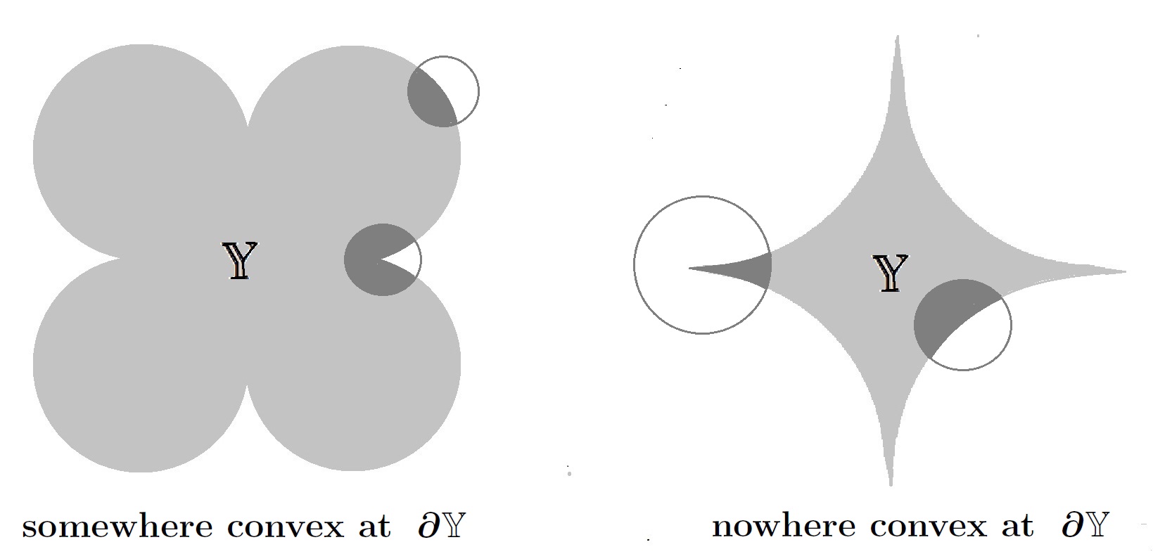
Figure 1. An illustration to Definition 1.7.

Theorem 1.8 (Uniqueness).

Under the assumptions in Theorem  1.5, if in addition $\,\mathbb{Y}\,$ is somewhere convex, then the Hopf-harmonic map $\,h\colon\overline{\mathbb{X}}\xrightarrow[]{{}_{\!\!\textnormal{onto\,\,}\!\!}}\overline{\mathbb{Y}}\,$ is unique.

In summary. Monotone Hopf harmonics open a new area of study in GFT with applications to the boundary value problems for hyper-elastic deformations of plates (planar domains) and thin films (surfaces in $\mathbb{R}^{3}$). This is the way to explain in mathematical rigor the principle of non-interpenetration of matter in NE. Topology of Monotone Sobolev mappings becomes a new resource in nonlinear PDEs.

2. Prerequisites

In this section we review from [41] useful concepts and results about Hopf differentials $h_{z}\overline{h_{\bar{z}}}\,\,\textnormal{d}z\otimes\textnormal{d}z$ and their trajectories. We, however, start with a powerful identity.

2.1. An identity

Lemma 2.1.

Let $\mathbb{X}$, $\mathbb{Y}$ and $\mathbb{G}$ be bounded domains in $\mathbb{C}$. Suppose that $h\colon\mathbb{G}\xrightarrow[]{{}_{\!\!\textnormal{onto\,\,}\!\!}}\mathbb{Y}$ and $H\colon\mathbb{\mathbb{X}}\xrightarrow[]{{}_{\!\!\textnormal{onto\,\,}\!\!}}\mathbb{Y}$ are orientation preserving $\mathscr{C}^{\infty}$-diffeomorphisms of finite Dirichlet energy. Define $\,f=H^{-1}\circ h\,\colon\mathbb{G}\xrightarrow[]{{}_{\!\!\textnormal{onto\,\,}\!\!}}\mathbb{X}$. Then we have

(2.1) $$\begin{split}\int_{\mathbb{X}}\lvert DH\rvert^{2}-\int_{\mathbb{G}}\lvert Dh\rvert^{2}&=4\int_{\mathbb{G}}\left[\frac{\lvert f_{z}-\sigma(z)f_{\bar{z}}\rvert^{2}}{\lvert f_{z}\rvert^{2}-\lvert f_{\bar{z}}\rvert^{2}}-1\right]\,\lvert h_{z}h_{\bar{z}}\rvert\,\textnormal{d}z\\ &+4\int_{\mathbb{G}}\frac{(\,\lvert h_{z}\rvert\,-\,\lvert h_{\bar{z}}\rvert\,)^{2}\cdot\lvert f_{\bar{z}}\rvert^{2}}{\lvert f_{z}\rvert^{2}-\lvert f_{\bar{z}}\rvert^{2}}\,\textnormal{d}z\end{split}$$

where

$$\sigma=\sigma(z)=\begin{cases}{h_{z}\overline{h_{\bar{z}}}}{\,\lvert h_{z}\overline{h_{\bar{z}}}\rvert^{-1}}\qquad&\textnormal{\;if }h_{z}\overline{h_{\bar{z}}}\neq 0\\ 0&\textnormal{\;otherwise.}\end{cases}$$

The integrals in (2.1) converge.

For the proof of Lemma 2.1 can be found in [17, Lemma 8.1].

The following simply connected (not necessarily Jordan) version of the Radó-Kneser-Choquet theorem will play a central role in our forthcoming arguments.

Lemma 2.2.

Consider a bounded simply connected domain $\mathbb{U}\subset\mathbb{C}$ and a bounded convex domain $\mathcal{Q}\subset\mathbb{C}$. Let $h\colon\partial\mathbb{U}\xrightarrow[]{{}_{\!\!\textnormal{onto\,\,}\!\!}}\partial\mathcal{Q}$ be a monotone mapping and $H\colon\mathbb{U}\to\mathbb{C}$ denote its harmonic extension. Then $H$ is a $\mathscr{C}^{\infty}$-diffeomorphism of $\mathbb{U}$ onto $\mathcal{Q}$.

The proof of this lemma we referee to [19].

2.2. Holomorphic quadratic differentials

Let $\varphi(z)\,\textnormal{d}z\otimes\textnormal{d}z$ be a holomorphic quadratic differential in $\mathbb{X}$ with isolated zeros, called critical points. Through every noncritical point there pass two $\mathscr{C}^{\infty}$-smooth orthogonal arcs. A vertical arc is a $\mathscr{C}^{\infty}$-smooth curve $\gamma=\gamma(t)$, $a<t<b$, along which

(2.2) $$[\dot{\gamma}(t)]^{2}\varphi\big{(}\gamma(t)\big{)}<0\,,\qquad\quad a<t<b\,.$$

A vertical trajectory of $\varphi$ in $\mathbb{X}$ is a maximal vertical arc, that is, not properly contained in any other vertical arc. The horizontal arcs and horizontal trajectories are defined in an exactly similar way, via the opposite inequality. Through every noncritical point of $\varphi$ there passes a unique vertical (horizontal) trajectory. A trajectory whose closure contains a critical point of $\varphi$ is called a critical trajectory. There are at most a countable number of critical trajectories.

Every noncritical vertical trajectory $\gamma\subset\mathbb{U}$ in a simply connected domain $\mathbb{U}$ is a cross cut, see Theorem 15.1 in [41].

Lemma 2.3.

Consider a vertical arc $\gamma\subset\mathbb{U}$ in a simply connected domain $\mathbb{U}$. Let $\beta$ be any locally rectifiable curve in $\mathbb{U}$ which contains the endpoints of $\gamma$. Then

(2.3) $$\int_{{\gamma}}\lvert\varphi\rvert^{\nicefrac{{1}}{{2}}}\,\lvert\textnormal{d}z\rvert\leqslant\int_{\beta}\lvert\varphi\rvert^{\nicefrac{{1}}{{2}}}\,\lvert\textnormal{d}z\rvert,$$

For the proof of this lemma we refer to [41, Theorem 16.1].

Lemma 2.4 (Fubini-like integration formula).

Let $\varphi(z)\,\textnormal{d}z\otimes\textnormal{d}z$ be a holomorphic quadratic differential in a simply connected domain $\mathbb{U}$, $\varphi\not\equiv 0$. Suppose that $F$ and $G$ are measurable functions in $\mathbb{U}$ such that

(2.4) $$\int_{\mathbb{U}}\lvert\varphi(z)\rvert\lvert F(z)\rvert\,\textnormal{d}z<\infty\quad\mbox{and}\quad\int_{\mathbb{U}}\lvert\varphi(z)\rvert\lvert G(z)\rvert\,\textnormal{d}z<\infty.$$

Then for almost every vertical trajectory $\gamma$ of $\varphi(z)\textnormal{d}z\otimes\textnormal{d}z$, we have

(2.5) $$\int_{\gamma}\lvert\varphi(z)\rvert^{\nicefrac{{1}}{{2}}}\lvert F(z)\rvert\,\lvert\textnormal{d}z\rvert<\infty\quad\mbox{and}\quad\int_{\gamma}\lvert\varphi(z)\rvert^{\nicefrac{{1}}{{2}}}\lvert G(z)\rvert\lvert\textnormal{d}z\rvert<\infty.$$

• If

  (2.6) $$\int_{\gamma}\lvert\varphi(z)\rvert^{\nicefrac{{1}}{{2}}}{F(z)}\,\lvert\textnormal{d}z\rvert=\int_{\gamma}\lvert\varphi(z)\rvert^{\nicefrac{{1}}{{2}}}{G(z)}\,\lvert\textnormal{d}z\rvert,$$

  for almost every vertical trajectory $\gamma$ of $\varphi(z)\,\textnormal{d}z\otimes\textnormal{d}z$ then

  (2.7) $$\int_{\mathbb{U}}\lvert\varphi(z)\rvert{F(z)}\,\textnormal{d}z=\int_{\mathbb{U}}\lvert\varphi(z)\rvert{G(z)}\,\textnormal{d}z$$

• If

  (2.8) $$\int_{\gamma}\lvert\varphi(z)\rvert^{\nicefrac{{1}}{{2}}}{F(z)}\,\lvert\textnormal{d}z\rvert\leqslant\int_{\gamma}\lvert\varphi(z)\rvert^{\nicefrac{{1}}{{2}}}{G(z)}\,\lvert\textnormal{d}z\rvert,$$

  for almost every vertical trajectory $\gamma$ of $\varphi(z)\textnormal{d}z\otimes\textnormal{d}z$ then

  (2.9) $$\int_{\mathbb{U}}\lvert\varphi(z)\rvert{F(z)}\,\textnormal{d}z\leqslant\int_{\mathbb{U}}\lvert\varphi(z)\rvert{G(z)}\,\textnormal{d}z$$

Again, for the proof we refer to [41]. The following proposition follows from [8, Proposition 5.1].

Proposition 2.5.

Suppose that a monotone mapping $h\colon\overline{\mathbb{X}}\xrightarrow[]{{}_{\!\!\textnormal{onto\,\,}\!\!}}\overline{\mathbb{Y}}$ solves the Hopf-Laplace equation

$$h_{z}\overline{h_{\bar{z}}}=\varphi\,,\qquad\textnormal{where }\varphi\textnormal{ is holomorphic in $\mathbb{X}$.}$$

Then the preimage $h^{-1}(y_{\circ})$ of a point $y_{\circ}\in\overline{\mathbb{Y}}$ is a continuum in $\overline{\mathbb{X}}$. If $h^{-1}(y_{\circ})$ intersects a noncritical vertical trajectory of $\varphi(z)\,\textnormal{d}z\otimes\textnormal{d}z$, then it lies entirely in that trajectory.

Given a quadratic holomorphic differential $\varphi(z)\,\textnormal{d}z\otimes\textnormal{d}z$ we define two partial differential operators, called the horizontal and vertical derivatives

$$\partial_{{}_{\mathsf{H}}}=\frac{\partial}{\partial z}+\frac{\varphi}{\lvert\varphi\rvert}\frac{\partial}{\partial\bar{z}}\qquad\mbox{ and }\qquad\partial_{{}_{\mathsf{V}}}=\frac{\partial}{\partial z}-\frac{\varphi}{\lvert\varphi\rvert}\frac{\partial}{\partial\bar{z}}.$$

If $h$ satisfies the Hopf-Laplace equation $h_{z}\overline{h_{\bar{z}}}=\varphi$, then the horizontal and vertical trajectories of $\varphi(z)\textnormal{d}z\otimes\textnormal{d}z$ are the lines of maximal and minimal stretch for $h$. Precisely, the following identities hold.

(2.10) $$\lvert\partial_{{}_{\mathsf{H}}}h\rvert=\lvert h_{z}\rvert+\lvert h_{\bar{z}}\rvert,\qquad\lvert\partial_{{}_{\mathsf{V}}}h\rvert=\big{|}\lvert h_{z}\rvert-\lvert h_{\bar{z}}\rvert\big{|}$$

(2.11) $$\lvert\partial_{{}_{\mathsf{H}}}h\rvert\cdot\lvert\partial_{{}_{\mathsf{V}}}h\rvert=\lvert J_{h}\rvert,\qquad\lvert\partial_{{}_{\mathsf{H}}}h\rvert^{2}-\lvert\partial_{{}_{\mathsf{V}}}h\rvert^{2}=4\lvert\varphi\rvert$$

Here and after $J_{h}=\det Dh$. As a consequence

(2.12) $$\lvert\partial_{{}_{\mathsf{V}}}h\rvert^{2}\leqslant\lvert J_{h}\rvert\leqslant\lvert\partial_{{}_{\mathsf{H}}}h\rvert^{2}.$$

Lemma 2.6.

Let $\Omega$ be an open subset in $\mathbb{C}$ and $h\colon\Omega\to\mathbb{C}$ a locally Lipschitz solution of the Hopf Laplace equation

$$h_{z}\overline{h_{\bar{z}}}=\varphi\,,\quad\textnormal{where }\varphi\textnormal{ is analytic in }\Omega\,.$$

Suppose that $J_{h}\equiv 0$ a.e. in $\Omega$. Then $h$ is constant on every vertical arc of the Hopf differential $\varphi(z)\,\textnormal{d}z\otimes\textnormal{d}z$.

Proof.

Choose and fix a vertical arc, say

$$\gamma=\{z(t)\colon a<t<b\,,\;\varphi(z(t))\dot{z}^{2}(t)<0\textnormal{ and }\lvert\dot{z}(t)\rvert\equiv 1\}\,.$$

Case 1. We say that $\gamma$ is a “good” vertical arc if for almost every $t\in(\alpha,\beta)$ the mapping $h$ is differentiable at $z(t)$ and $J_{h}\big{(}z(t)\big{)}=0$. We begin with the chain rule along a “good” vertical arc,

$$\frac{\textnormal{d}}{\textnormal{d}t}h\big{(}z(t)\big{)}=h_{z}\big{(}z(t)\big{)}\dot{z}(t)+h_{\bar{z}}\big{(}z(t)\big{)}\overline{\dot{z}(t)}\,.$$

Hence

$$\begin{split}\Big{|}\frac{\textnormal{d}}{\textnormal{d}t}h\big{(}z(t)\big{)}\Big{|}^{2}&=\lvert h_{z}\big{(}z(t)\big{)}\rvert^{2}+\lvert h_{\bar{z}}\big{(}z(t)\big{)}\rvert^{2}\\ &+h_{z}\big{(}z(t)\big{)}\overline{h_{\bar{z}}\big{(}z(t)\big{)}}\dot{z}^{2}(t)+\overline{h_{z}\big{(}z(t)\big{)}\overline{h_{\bar{z}}\big{(}z(t)\big{)}}\dot{z}^{2}(t)}\end{split}$$

Since $\gamma$ is a vertical arc the function defined by

$$\gamma(t)\stackrel{{\scriptstyle\textnormal{def}}}{{=\!\!=}}\varphi\big{(}z(t)\big{)}\dot{z}^{2}(t)$$

is smooth real-valued and negative. Clearly, for almost every $\alpha<t<\beta$ we have $\varphi\big{(}z(t)\big{)}=h_{z}\big{(}z(t)\big{)}\overline{h_{\bar{z}}\big{(}z(t)\big{)}}$ and

$$\lvert\gamma(t)\rvert=\lvert h_{z}\big{(}z(t)\big{)}\rvert\,\lvert h_{\bar{z}}\big{(}z(t)\big{)}\rvert=\lvert h_{z}\big{(}z(t)\big{)}\rvert^{2}=\lvert h_{\bar{z}}\big{(}z(t)\big{)}\rvert^{2}\,,$$

because the Jacobian determinant $J_{h}\big{(}z(t)\big{)}=\lvert h_{z}\big{(}z(t)\big{)}\rvert^{2}-\lvert h_{\bar{z}}\big{(}z(t)\big{)}\rvert^{2}$ vanishes. We conclude with the equation

$$\Big{|}\frac{\textnormal{d}}{\textnormal{d}t}h\big{(}z(t)\big{)}\Big{|}^{2}=\lvert\gamma(t)\rvert+\lvert\gamma(t)\rvert+\gamma(t)+\gamma(t)=0\,\qquad\textnormal{for a.e. }t\in(\alpha,\beta)\,.$$

Hence $h\big{(}z(t)\big{)}$ is constant on $\gamma$.
Case 2. Now, let $\gamma$ be an arbitrary vertical arc. It suffices to show that $h$ is locally constant on $\gamma$, say on $\gamma\cap\mathcal{R}$, where $\mathcal{R}$ is a curved rectangular box swept out by vertical arcs (as well as by horizontal arcs). Upon a conformal change of variables, locally defined by the rule $\xi=\int\sqrt{\varphi(z)}\,\textnormal{d}z$, we see that $\mathcal{R}$ becomes an Euclidean rectangle, denoted by $\mathcal{R}^{\ast}$. The vertical and horizontal arcs of $\varphi(z)\,\textnormal{d}z\otimes\textnormal{d}z$ become vertical and horizontal straight segments of $\mathcal{R}^{\ast}$, respectively. The new function $h^{\ast}(\xi)\stackrel{{\scriptstyle\textnormal{def}}}{{=\!\!=}}h\big{(}z(\xi)\big{)}$ gives rise to the Hopf quadratic differential on $\mathcal{R}^{\ast}$

$$\varphi^{\ast}(\xi)\,\textnormal{d}\xi\otimes\textnormal{d}\xi\,,\qquad\textnormal{where }\varphi^{\ast}(\xi)=h^{\ast}_{\xi}\,\overline{h^{\ast}_{\bar{\xi}}}$$

whose trajectories are the vertical and horizontal segments. Also, $J_{h^{\ast}}(\xi)=0$ for almost every $\xi\in\mathcal{R}^{\ast}$. By Fubini’s theorem almost every vertical segment is a “good” vertical arc of the differential $\varphi^{\ast}(\xi)\,\textnormal{d}\xi\otimes\textnormal{d}\xi$. By Case 1., $h^{\ast}$ is constant on almost every vertical segment of $\mathcal{R}^{\ast}$. Finally, since $h^{\ast}$ is continuous, it is constant on every vertical segment. This means that $h$ is constant on every vertical arc in $\mathcal{R}$, as desired. ∎

3. Proof of Theorem 1.5

3.1. Setting and notation

Let $g\colon\overline{\mathbb{X}}\xrightarrow[]{{}_{\!\!\textnormal{onto\,\,}\!\!}}\overline{\mathbb{Y}}$ be given as in Theorem 1.5. We denote the class of monotone mappings $H\colon\overline{\mathbb{X}}\xrightarrow[]{{}_{\!\!\textnormal{onto\,\,}\!\!}}\overline{\mathbb{Y}}$ in the Sobolev space $\mathscr{W}^{1,2}(\mathbb{X},\mathbb{C})$ which coincide with $g$ on $\partial\mathbb{X}$ by $\mathscr{M}_{g}(\overline{\mathbb{X}},\overline{\mathbb{Y}})$. Furthermore, we write

$$\mathscr{H}_{g}(\overline{\mathbb{X}},\overline{\mathbb{Y}})=\{H\in\mathscr{M}_{g}(\overline{\mathbb{X}},\overline{\mathbb{Y}})\colon H\colon\overline{\mathbb{X}}\xrightarrow[]{{}_{\!\!\textnormal{onto\,\,}\!\!}}\overline{\mathbb{Y}}\textnormal{ is a homeomorphism}\}$$

and

$$\operatorname{Diff}_{g}(\overline{\mathbb{X}},\overline{\mathbb{Y}})=\{H\in\mathscr{M}_{g}(\overline{\mathbb{X}},\overline{\mathbb{Y}})\colon H\colon{\mathbb{X}}\xrightarrow[]{{}_{\!\!\textnormal{onto\,\,}\!\!}}{\mathbb{Y}}\textnormal{ is a diffeomorphism}\}\,.$$

Clearly, $\mathscr{H}_{g}(\overline{\mathbb{X}},\overline{\mathbb{Y}})$ is non empty, because it contains $g\colon\overline{\mathbb{X}}\xrightarrow[]{{}_{\!\!\textnormal{onto\,\,}\!\!}}\overline{Y}$. Now, the direct method in the Calculus of Variations reveals that there always exists $h\in\mathscr{M}_{g}\,(\overline{\mathbb{X}},\overline{\mathbb{Y}})$ with smallest Dirichlet energy. Indeed, the energy-minimizing sequence of monotone mappings in $\mathscr{M}_{g}(\overline{\mathbb{X}},\overline{\mathbb{Y}})$ converges weakly in $\mathscr{W}^{1,2}(\mathbb{X},\mathbb{C})$ and it converges uniformly to a monotone mapping $h\in\mathscr{M}_{g}\,(\overline{\mathbb{X}},\overline{\mathbb{Y}})$. The uniform convergence will follow from a general observation, see Remark 3.1.

Furthermore, the energy of $h$ equals exactly the infimum of the energy among all homeomorphisms in $\mathscr{H}_{g}(\overline{\mathbb{X}},\overline{\mathbb{Y}})$. In symbols,

(3.1) $$\min_{H\in\mathscr{M}_{g}(\overline{\mathbb{X}},\overline{\mathbb{Y}})}\int_{\mathbb{X}}|DH(x)|^{2}\,\textnormal{d}x=\inf_{H\in\mathscr{H}_{g}(\overline{\mathbb{X}},\overline{\mathbb{Y}})}\int_{\mathbb{X}}|DH(x)|^{2}\,\textnormal{d}x\,.$$

This follows from a Sobolev variant of Youngs’ approximation theorem [18]. Also, according to the approximation result [13], the infimum energy among diffeomorphisms leads to the same minimum value. Precisely, the equation (3.1) extends as

(3.2) $$\inf_{H\in\mathscr{H}_{g}(\overline{\mathbb{X}},\overline{\mathbb{Y}})}\int_{\mathbb{X}}|DH(x)|^{2}\,\textnormal{d}x=\inf_{H\in\operatorname{Diff}_{g}(\overline{\mathbb{X}},\overline{\mathbb{Y}})}\int_{\mathbb{X}}|DH(x)|^{2}\,\textnormal{d}x\,.$$

Remark 3.1.

Every homeomorphism $g\colon\mathbb{X}\xrightarrow[]{{}_{\!\!\textnormal{onto\,\,}\!\!}}\mathbb{Y}$ between planar Jordan domains (not necessarily simply connected) admits a unique continuous extension as a map from $\overline{\mathbb{X}}$ onto $\overline{\mathbb{Y}}$, still denoted by $g\colon\overline{\mathbb{X}}\xrightarrow[]{{}_{\!\!\textnormal{onto\,\,}\!\!}}\overline{\mathbb{Y}}$. The extension is monotone. Also the boundary map $g\colon\partial\mathbb{X}\xrightarrow[]{{}_{\!\!\textnormal{onto\,\,}\!\!}}\partial\mathbb{Y}$ is monotone. Now consider a general monotone map $g\colon\overline{\mathbb{X}}\xrightarrow[]{{}_{\!\!\textnormal{onto\,\,}\!\!}}\overline{\mathbb{Y}}$ (not necessarily an extension of a homeomorphism) and assume that $\mathbb{Y}$ is Lipschitz regular; that is, locally $\partial\mathbb{Y}$ becomes a graph of a Lipschitz function upon suitable rotation. Then we have the following uniform bound of the modulus of continuity of every monotone map $g\in\mathscr{W}^{1,2}(\mathbb{X},\mathbb{R}^{2})$

(3.3) $$\lvert g(x_{1})-g(x_{2})\rvert^{2}\leqslant C_{\mathbb{X},\mathbb{Y}}\frac{\int_{\mathbb{X}}\lvert Dg(x)\rvert^{2}\,\textnormal{d}x}{\log\left(e+1/\lvert x_{1}-x_{2}\rvert\right)}$$

for all $x_{1},x_{2}\in\overline{\mathbb{X}}$. Here the constant $C_{\mathbb{X},\mathbb{Y}}$ depends only on the domains $\mathbb{X}$ and $\mathbb{Y}$, but not on the mapping $g$. The proof of (3.3) can be found in [16]. This estimate shows that a family of monotone mappings $g\colon\overline{\mathbb{X}}\xrightarrow[]{{}_{\!\!\textnormal{onto\,\,}\!\!}}\overline{\mathbb{Y}}$ which is bounded in $\mathscr{W}^{1,2}(\mathbb{X},\mathbb{R}^{2})$ is equicontinuous. In particular, every sequence in this family contains a subsequence converging uniformly and weakly in $\mathscr{W}^{1,2}(\mathbb{X},\mathbb{R}^{2})$ to a monotone map from $\overline{\mathbb{X}}$ onto $\overline{\mathbb{Y}}$ in the Sobolev class $\mathscr{W}^{1,2}(\mathbb{X},\mathbb{R}^{2})$.

3.2. Existence

The existence of Hopf-harmonic monotone mapping $h$ in Theorem 1.5 will be achieved by minimizing the Dirichlet-energy within the class $\mathscr{M}_{g}(\overline{\mathbb{X}},\overline{\mathbb{Y}})$. First, note that the existence of mapping with smallest Dirichlet-energy in $\mathscr{M}_{g}(\overline{\mathbb{X}},\overline{\mathbb{Y}})$ follows from (3.1). Second, the standard outer variation does not apply to this mapping. But one can perform the inner variation, a change of variables in $\mathbb{X}$,

$$\frac{\textnormal{d}}{\textnormal{d}t}\bigg{|}_{t=0}\mathcal{E}_{\mathbb{X}}[h\circ\eta_{t}]=0$$

Here $\eta_{t}\colon\mathbb{X}\xrightarrow[]{{}_{\!\!\textnormal{onto\,\,}\!\!}}\mathbb{X}$ is a family of diffeomorphisms $\eta_{t}\colon\mathbb{X}\xrightarrow[]{{}_{\!\!\textnormal{onto\,\,}\!\!}}\mathbb{X}$ depending smoothly on the parameter $t\in\mathbb{R}$ which extend continuously up to $\overline{\mathbb{X}}$ as the identity map on $\partial\mathbb{X}$. The inner variation leads us to the claimed Hopf-Laplace equation [23] [17, §3.1],

$$\frac{\partial}{\partial\bar{z}}(h_{z}\overline{h_{\bar{z}}})=0\,,\qquad h\in\mathscr{M}_{g}(\overline{\mathbb{X}},\overline{\mathbb{Y}})\,.$$

3.3. Lipschitz Regularity

The Lipschitz regularity follows from the work [15] which, among other things, tells us that a solution to the Hopf-Laplace equation (1.1) with non-negative Jacobian $J(x,h)\geqslant 0$, a.e., is a locally Lipschitz mapping. The fact that a monotone mapping $h\in\mathscr{M}_{g}(\overline{\mathbb{X}},\overline{\mathbb{Y}})$ has $J(x,h)\geqslant 0$, a.e., follows from the approximation result in [18]. Indeed, there exists a sequence of diffeomorphims $h_{j}\in\operatorname{Diff}_{g}(\overline{\mathbb{X}},\overline{\mathbb{Y}})$ such that $h_{j}\to h$ in $\mathscr{W}^{1,2}(\mathbb{X},\mathbb{C})$. Now, $J(x,h_{j})\geqslant 0$ because $g\colon\partial\mathbb{X}\xrightarrow[]{{}_{\!\!\textnormal{onto\,\,}\!\!}}\partial\mathbb{Y}$ is positively oriented. Combining this with the fact that $J(x,h_{j})\to J(x,h)$ a.e. in $\mathbb{X}$, the claimed inequality $J(x,h)\geqslant 0$ follows.

3.4. Partial harmonicity

This term refers to the fact that $h$ restricted to $h^{-1}(\mathbb{Y})\subset\mathbb{X}$ is a harmonic diffeomorphism. To see this we may assume that the Hopf product $h_{z}\overline{h_{\bar{z}}}=\varphi$ does not vanish identically for otherwise $h$ would be holomorphic in $\mathbb{X}$. This is immediately from the estimate

$$\lvert h_{\bar{z}}\rvert^{2}\leqslant\lvert h_{z}\overline{h_{\bar{z}}}\rvert=0\,.$$

Let $\mathbb{D}$ be any open convex subdomain in $\mathbb{Y}$, for instance any open disk and $\mathbb{U}=h^{-1}(\mathbb{D})$. According to Lemma 2.8 and 2.9 in [18] $\mathbb{U}$ is simply connected (not necessarily Jordan) and the boundary mapping $h\colon\partial\mathbb{U}\xrightarrow[]{{}_{\!\!\textnormal{onto\,\,}\!\!}}\partial\mathbb{D}$ is monotone. We appeal to a Radó-Kneser-Choquet result for simply connected domains, see Lemma 2.2. Accordingly, the harmonic extension of the boundary mapping $h\colon\partial\mathbb{U}\xrightarrow[]{{}_{\!\!\textnormal{onto\,\,}\!\!}}\partial\mathbb{D}$ to $\mathbb{U}$, is $\mathscr{C}^{\infty}$-diffeomorphism of $\mathbb{U}$ onto $\mathbb{D}$, denoted by $H\colon\mathbb{U}\xrightarrow[]{{}_{\!\!\textnormal{onto\,\,}\!\!}}\mathbb{D}$. We will prove the opposite inequality,

(3.4) $$\mathcal{E}_{\mathbb{U}}[h]=\int_{\mathbb{U}}\lvert Dh\rvert^{2}\leqslant\int_{\mathbb{U}}\lvert DH\rvert^{2}=\mathcal{E}_{\mathbb{U}}[H]\,.$$

Before passing to the proof of this inequality let us show how it would imply the partial harmonicity of $h$. Obviously,

$$\int_{\mathbb{U}}\lvert DH\rvert^{2}\leqslant\int_{\mathbb{U}}\lvert Dh\rvert^{2}\,.$$

This shows that $h=H$ in $\mathbb{U}$ and therefore $h$ is a harmonic diffeomorphism of $\mathbb{U}$ onto $\mathbb{D}$. This property applies to every disk $\mathbb{D}\subset\mathbb{Y}$ and, consequently, $h$ is a local diffeomorphism. On the other hand, the mapping $h$ being monotone, is actually a global diffeomorphism from $h^{-1}({\mathbb{Y}})$ onto $\mathbb{Y}$.

3.4.1. Proof of the inequality (3.4)

The proof is based on the following consequence of Lemma 2.1.

Lemma 3.2.

Let $f=H^{-1}\circ h\colon\mathbb{U}\xrightarrow[]{{}_{\!\!\textnormal{onto\,\,}\!\!}}\mathbb{U}$ and $\varphi=h_{z}\overline{h_{\bar{z}}}$. Then we have

(3.5) $$\begin{split}\mathcal{E}_{\mathbb{U}}[H]-\mathcal{E}_{\mathbb{U}}[h]&\geqslant\frac{4}{\lVert\varphi\rVert_{\mathscr{L}^{1}(\mathbb{U})}}\,\left[\int_{\mathbb{U}}\Big{\lvert}f_{z}-\frac{\varphi}{\lvert\varphi\rvert}f_{\bar{z}}\Big{\rvert}\,\sqrt{\lvert\varphi\rvert}\sqrt{\lvert\varphi\big{(}f\big{)}\rvert}\right]^{2}\\ &-4\int_{\mathbb{U}}\lvert\varphi\rvert.\end{split}$$

Here we assume that $\varphi\not\equiv 0$. The term $\frac{\varphi}{\lvert\varphi\rvert}$ is understood as equal to zero at the points where $\varphi$ vanishes.

Proof.

By the approximation result in [18], there exist a sequence of diffeomorphisms $h^{j}\colon\mathbb{U}\xrightarrow[]{{}_{\!\!\textnormal{onto\,\,}\!\!}}\mathbb{D}$, converging to $h$ uniformly and in $\mathscr{W}^{1,2}(\mathbb{U},\mathbb{C})$. Moreover, each $h^{j}$ extends continuously to $\overline{\mathbb{U}}$ with $h^{j}=h$ on $\partial\mathbb{U}$. Let $\mathbb{U}^{\prime}$ be a compactly contained subdomain of $\mathbb{U}$. Write $f^{j}=H^{-1}\circ h^{j}\colon\mathbb{U}\xrightarrow[]{{}_{\!\!\textnormal{onto\,\,}\!\!}}\mathbb{U}$. Applying Lemma 2.1 we obtain

(3.6) $$\begin{split}\int_{f^{j}(\mathbb{U}^{\prime})}\lvert DH\rvert^{2}-\int_{\mathbb{U}^{\prime}}\lvert Dh^{j}\rvert^{2}&=4\int_{\mathbb{U}^{\prime}}\left[\frac{\lvert f^{j}_{z}-\sigma^{j}(z)f^{j}_{\bar{z}}\rvert^{2}}{\lvert f^{j}_{z}\rvert^{2}-\lvert f^{j}_{\bar{z}}\rvert^{2}}-1\right]\,\lvert h^{j}_{z}\,h^{j}_{\bar{z}}\rvert\\ &+4\int_{\mathbb{U}^{\prime}}\frac{(\,\lvert h^{j}_{z}\rvert\,-\,\lvert h^{j}_{\bar{z}}\rvert\,)^{2}\cdot\lvert f^{j}_{\bar{z}}\rvert^{2}}{\lvert f^{j}_{z}\rvert^{2}-\lvert f^{j}_{\bar{z}}\rvert^{2}}\,,\end{split}$$

where

$$\sigma^{j}=\sigma^{j}(z)=\begin{cases}{h^{j}_{z}\,\overline{h^{j}_{\bar{z}}}}{\;\lvert h^{j}_{z}\,\overline{h^{j}_{\bar{z}}}\rvert^{-1}}\qquad&\textnormal{\;if }h^{j}_{z}\overline{h^{j}_{\bar{z}}}\neq 0\\ 0&\textnormal{\;otherwise.}\end{cases}$$

Since $f^{j}$ are sense-preserving diffeomorphisms, the last integral in (3.6) is nonnegative,

$$\int_{\mathbb{U}^{\prime}}\frac{(\,\lvert h^{j}_{z}\rvert\,-\,\lvert h^{j}_{\bar{z}}\rvert\,)^{2}\cdot\lvert f^{j}_{\bar{z}}\rvert^{2}}{\lvert f^{j}_{z}\rvert^{2}-\lvert f^{j}_{\bar{z}}\rvert^{2}}\,\textnormal{d}z\geqslant 0\,.$$

We estimate the first integral by Hölder’s inequality,

$$\int_{\mathbb{U}^{\prime}}\frac{\lvert f^{j}_{z}-\sigma^{j}(z)f^{j}_{\bar{z}}\rvert^{2}}{\lvert f^{j}_{z}\rvert^{2}-\lvert f^{j}_{\bar{z}}\rvert^{2}}\,\lvert h^{j}_{z}\,h^{j}_{\bar{z}}\rvert\,\textnormal{d}z\geqslant\frac{\left(\int_{\mathbb{U}^{\prime}}\,\lvert f^{j}_{z}-\sigma^{j}f^{j}_{\bar{z}}\rvert\sqrt{\lvert h^{j}_{z}\,h^{j}_{\bar{z}}\rvert}\,\sqrt{\lvert\varphi(f^{j}(z))\rvert}\,\textnormal{d}z\right)^{2}}{\int_{\mathbb{U}^{\prime}}J(z,f^{j})\,\lvert\varphi(f^{j}(z))\rvert\,\textnormal{d}z}$$

The denominator is bounded from above, by the $\mathscr{L}^{1}$-norm of $\varphi$,

$$\int_{\mathbb{U}^{\prime}}J(z,f^{j})\,\lvert\varphi(f^{j}(z))\rvert\,\textnormal{d}z=\int_{f^{j}(\mathbb{U}^{\prime})}\lvert\varphi\rvert\leqslant\int_{\mathbb{U}}\lvert\varphi\rvert$$

Since $\mathbb{U}\supset f^{j}(\mathbb{U})$ for sufficiently large $j$, we have

(3.7) $$\begin{split}\mathcal{E}_{\mathbb{U}}[H]-\mathcal{E}_{\mathbb{U}^{\prime}}[h^{j}]&\geqslant 4\,\frac{\left(\int_{\mathbb{U}^{\prime}}\,\lvert f^{j}_{z}-\sigma^{j}f^{j}_{\bar{z}}\rvert\sqrt{\lvert h^{j}_{z}h^{j}_{\bar{z}}\rvert}\,\sqrt{\lvert\varphi(f^{j}(z))\rvert}\,\textnormal{d}z\right)^{2}}{\int_{\mathbb{U}}\lvert\varphi\rvert\,\textnormal{d}z}\\ &-4\,\int_{\mathbb{U}^{\prime}}\lvert h^{j}_{z}h^{j}_{\bar{z}}\rvert\,\textnormal{d}z\end{split}$$

Next, we let $j\to\infty$. We may assume, passing to a subsequence if necessary, that $h^{j}_{z}$ and $h^{j}_{\bar{z}}$ converge almost everywhere to $h_{z}$ and $h_{\bar{z}}$, respectively. Since the sequence $f^{j}=H^{-1}\circ h^{j}\colon\mathbb{U}\xrightarrow[]{{}_{\!\!\textnormal{onto\,\,}\!\!}}\mathbb{U}$ is converging to $f$ uniformly and in $\mathscr{W}^{1,2}(\mathbb{U}^{\prime})$ on subdomains $\mathbb{U}^{\prime}\Subset\mathbb{U}$, it follows that

$$\lvert f_{z}^{j}-\sigma^{j}f^{j}_{\bar{z}}\rvert\,\sqrt{\lvert h^{j}_{z}h^{j}_{\bar{z}}\rvert}\;\to\;\lvert f_{z}-\sigma f_{\bar{z}}\rvert\sqrt{\lvert h_{z}h_{\bar{z}}\rvert}\qquad\textnormal{in }\mathscr{L}^{1}(\mathbb{U}^{\prime})$$

and

$$\sqrt{\lvert\varphi(f^{j}(z))\rvert}\to\sqrt{\lvert\varphi(f(z))\rvert}\,,\quad\textnormal{everywhere.}$$

Combining these facts with (3.7), we conclude

$$\mathcal{E}_{\mathbb{U}}[H]-\mathcal{E}_{\mathbb{U}^{\prime}}[h]\geqslant 4\frac{\left[\int_{\mathbb{U}^{\prime}}\left|f_{z}-\sigma f_{\bar{z}}\right|\,\sqrt{\lvert\varphi(z)\rvert}\,\sqrt{\lvert\varphi\big{(}f(z)\big{)}\rvert}\,\textnormal{d}z\right]^{2}}{\int_{\mathbb{U}}\lvert\varphi(z)\rvert\,\textnormal{d}z}-4\int_{\mathbb{U}^{\prime}}\lvert\varphi\rvert.$$

Finally, since $\mathbb{U}^{\prime}$ was an arbitrary compact subset of $\mathbb{U}$, Lemma 3.2 follows. ∎

Now having Lemma 3.2, the inequality (3.4) would follow provided we can show that

(3.8) $$\int_{\mathbb{U}}\Big{\lvert}f_{z}-\frac{\varphi}{\lvert\varphi\rvert}f_{\bar{z}}\Big{\rvert}\,\sqrt{\lvert\varphi\rvert}\,\sqrt{\lvert\varphi\circ f\rvert}\,\textnormal{d}z\geqslant\int_{\mathbb{U}}\lvert\varphi\rvert\,\textnormal{d}z$$

Proof of (3.8).

For almost every vertical noncritical trajectory $\gamma$, the mapping $f$ is locally absolutely continuous on $\gamma$. Let $\hat{\gamma}$ be a maximal subarc of $\gamma$ which lies in $\mathbb{U}$ so its endpoints belong to $\partial\mathbb{U}$. Now, the change of variable formula gives

(3.9) $$\int_{\hat{\gamma}}\Big{\lvert}f_{z}-\frac{\varphi}{\lvert\varphi\rvert}f_{\bar{z}}\Big{\rvert}\,\sqrt{\lvert\varphi\circ f\rvert}=\int_{\hat{\gamma}}\lvert f_{{}_{\mathsf{V}}}\rvert\sqrt{\lvert\varphi\circ f\rvert}=\int_{f(\hat{\gamma})}\sqrt{\lvert\varphi\rvert}\,.$$

Applying Lemma 2.3 to the curve $\beta=f(\hat{\gamma})$ we have

$$\int_{f(\hat{\gamma})}\sqrt{\varphi}\geqslant\int_{\hat{\gamma}}\sqrt{\varphi}\,.$$

Combining this estimate with (3.9), we obtain

$$\int_{\hat{\gamma}}\Big{\lvert}f_{z}-\frac{\varphi}{\lvert\varphi\rvert}f_{\bar{z}}\Big{\rvert}\,\sqrt{\lvert\varphi\circ f\rvert}\geqslant\int_{\hat{\gamma}}\sqrt{\varphi}\,.$$

Now, the claimed inequality (3.8) follows from this by the Fubini formula of integration, see (2.8)–(2.9). ∎

This also completes the proof of (3.4) and proves partial harmonicity. In general $h^{-1}(\mathbb{Y})$ may or may not touch the boundary of $\mathbb{X}$. It is exactly at this point the somewhere convexity of $\mathbb{Y}$ comes into play.

Lemma 3.3.

Suppose that $\mathbb{Y}$ is somewhere convex and $h\colon\overline{\mathbb{X}}\xrightarrow[]{{}_{\!\!\textnormal{onto\,\,}\!\!}}\overline{\mathbb{Y}}$ is a monotone Hopf-harmonic mapping. Then $h^{-1}(\mathbb{Y})$ touches $\partial\mathbb{X}$ along an open arc. Precisely $\overline{h^{-1}(\mathbb{Y})}$ contains an open arc of $\partial\mathbb{X}$.

Proof.

Recall that the somewhere convexity of $\mathbb{Y}$ means that there is an open disk $\mathbb{D}$ centered at $y_{\circ}\in\partial\mathbb{Y}$ so that the intersection $\mathbb{D}\cap\mathbb{Y}$ (called boundary cell) is a convex set. Denote it by $\mathcal{Q}=\mathbb{D}\cap\mathbb{Y}$. We introduce the so-called sealed boundary cell $\mathcal{Q}^{+}\stackrel{{\scriptstyle\textnormal{def}}}{{=\!\!=}}\mathbb{D}\cap\overline{\mathbb{Y}}$. Thus $\mathcal{Q}^{+}=\mathcal{Q}\cup\mathcal{C}$, where $\mathcal{C}=\mathbb{D}\cap\partial\mathbb{Y}$ is an open arc in $\partial\mathbb{Y}$. Clearly, $\mathcal{Q}^{+}$ is a connected subset of $\overline{\mathbb{Y}}$. Consider the preimage of the sealed boundary cell

$$\mathcal{U}^{+}\stackrel{{\scriptstyle\textnormal{def}}}{{=\!\!=}}h^{-1}(\mathcal{Q}^{+})\subset\overline{\mathbb{X}}\,.$$

Since $h\colon\overline{\mathbb{X}}\xrightarrow[]{{}_{\!\!\textnormal{onto\,\,}\!\!}}\overline{\mathbb{Y}}$ is monotone, $\mathcal{U}^{+}$ is connected. Now we have $\mathcal{U}^{+}=\mathcal{U}\cup\Gamma$, where $\mathcal{U}=h^{-1}(\mathcal{Q}^{+})\cap\mathbb{X}$ is a simply connected domain and $\Gamma=h^{-1}(\mathcal{Q}^{+})\cap\partial\mathbb{X}$ is an open arc in $\partial\mathbb{X}$. Moreover, the mapping $h\colon\partial\mathcal{U}\xrightarrow[]{{}_{\!\!\textnormal{onto\,\,}\!\!}}\partial\mathcal{Q}$ is monotone. We refer to [18] for the proof of these topological facts. It should be emphasized that $h^{-1}(\mathcal{Q})$ need not be equal to $\mathcal{U}$.

In much the same way as in the proof of partial harmonicity, we appeal to the Radó-Kneser-Choquet theorem for simply connected domain, see Lemma 2.2. Accordingly, let $H\colon\mathcal{U}\xrightarrow[]{{}_{\!\!\textnormal{onto\,\,}\!\!}}\mathcal{Q}$ be the harmonic extension of the boundary mapping $h\colon\partial\mathcal{U}\xrightarrow[]{{}_{\!\!\textnormal{onto\,\,}\!\!}}\partial\mathcal{Q}$. Now, the proof of the inequality (3.4) in §3.4.1 goes in similar lines, namely we obtain

$$\int_{\mathcal{U}}\lvert Dh\rvert^{2}\leqslant\int_{\mathcal{U}}\lvert DH\rvert^{2}$$

and conclude that $h=H$ on $\mathcal{U}$. This amounts to saying that

$$h^{-1}({\mathbb{Y}})\supset\mathcal{U}\textnormal{ which touches }\partial\mathbb{X}\textnormal{ along }\Gamma\,.$$

∎

Before proceeding the uniqueness of Hopf-harmonic monotone mappings, a proof of Theorem 1.8, let us give an equivalent characterization for maps in question. In Section 3.2 we showed that a mapping $h\colon\overline{\mathbb{X}}\xrightarrow[]{{}_{\!\!\textnormal{onto\,\,}\!\!}}\overline{\mathbb{Y}}$ which minimizes the Dirichlet energy among Sobolev monotone mapping in $\mathscr{M}_{g}(\overline{\mathbb{X}},\overline{\mathbb{Y}})$ is a Hopf-harmonic monotone mapping. Actually, the converse also holds.

3.5. Monotone Hopf-harmonics are the energy minimizers

Proposition 3.4.

Let $\mathbb{Y}$ be a simply connected Lipschitz domain in $\mathbb{C}$ and $g\colon\overline{\mathbb{X}}\xrightarrow[]{{}_{\!\!\textnormal{onto\,\,}\!\!}}\overline{\mathbb{Y}}$ be an orientation-preserving homeomorphism of a Sobolev class $\mathscr{W}^{1,2}(\mathbb{X},\mathbb{C})$, defined on a Jordan domain $\mathbb{X}$. Then $h\in\mathscr{M}_{g}(\overline{\mathbb{X}},\overline{\mathbb{Y}})$ is Hopf-harmonic if and only if

$$\begin{split}\int_{\mathbb{X}}\lvert Dh(x)\rvert^{2}\,\textnormal{d}x&=\min_{H\in\mathscr{M}_{g}(\overline{\mathbb{X}},\overline{\mathbb{Y}})}\int_{\mathbb{X}}|DH(x)|^{2}\,\textnormal{d}x\\ &=\inf_{H\in\operatorname{Diff}_{g}(\overline{\mathbb{X}},\overline{\mathbb{Y}})}\int_{\mathbb{X}}|DH(x)|^{2}\,\textnormal{d}x\,.\end{split}$$

Here, the last equality follows from (3.1) and (3.2).

Proof.

Let $h\in\mathscr{M}_{g}(\overline{\mathbb{X}},\overline{\mathbb{Y}})$ be a Hopf-harmonic mapping. Then

$$h_{z}\overline{h_{\bar{z}}}=\varphi\qquad\textnormal{for some holomorphic }\varphi\not\equiv 0\,.$$

Let $\mathbb{G}=h^{-1}(\mathbb{Y})$. In view of partial harmonicity in Section 3.4, the mapping $h\colon\overline{\mathbb{X}}\xrightarrow[]{{}_{\!\!\textnormal{onto\,\,}\!\!}}\overline{\mathbb{Y}}$ is a harmonic diffeomorphism from $\mathbb{G}$ onto $\mathbb{Y}$. Let $H\in\operatorname{Diff}_{g}(\overline{\mathbb{X}},\overline{\mathbb{Y}})$. Define

$$f=H^{-1}\circ h\colon\mathbb{G}\xrightarrow[]{{}_{\!\!\textnormal{onto\,\,}\!\!}}\mathbb{X}\,.$$

In view of Lemma 2.1, we see that

$$\begin{split}\mathcal{E}_{\mathbb{X}}[H]-\mathcal{E}_{\mathbb{G}}[h]&=4\int_{\mathbb{G}}\left[\frac{\lvert f_{z}-\frac{\varphi}{\lvert\varphi\rvert}f_{\bar{z}}\rvert^{2}}{\lvert f_{z}\rvert^{2}-\lvert f_{\bar{z}}\rvert^{2}}-1\right]\,\lvert\varphi\rvert\,\textnormal{d}z\\ &+4\int_{\mathbb{G}}\frac{(\,\lvert h_{z}\rvert\,-\,\lvert h_{\bar{z}}\rvert\,)^{2}\cdot\lvert f_{\bar{z}}\rvert^{2}}{\lvert f_{z}\rvert^{2}-\lvert f_{\bar{z}}\rvert^{2}}\,\textnormal{d}z\\ &=4\int_{\mathbb{G}}\left[\frac{\lvert\partial_{{}_{\mathsf{V}}}f\rvert^{2}}{J_{f}}-1\right]\,\lvert\varphi\rvert\,\textnormal{d}z\\ &+4\int_{\mathbb{G}}\frac{(\,\lvert h_{z}\rvert\,-\,\lvert h_{\bar{z}}\rvert\,)^{2}\cdot\lvert f_{\bar{z}}\rvert^{2}}{J_{f}}\,\textnormal{d}z\end{split}$$

Before going further, let us observe that

$$\int_{\mathbb{X}\setminus\mathbb{G}}\lvert Dh\rvert^{2}=4\int_{\mathbb{X}\setminus\mathbb{G}}\lvert\varphi\rvert\,.$$

Indeed, since $J_{h}\geqslant 0$ a.e. in $\mathbb{X}$ and $h$ belongs to the Sobolev class $\mathscr{W}^{1,2}(\mathbb{X},\mathbb{C})$, it follows that $J_{h}=0$ a.e. in $\mathbb{X}\setminus\mathbb{G}=h^{-1}{\partial\mathbb{Y}}$. This is because $h(\mathbb{X}\setminus\mathbb{G})\subset\partial\mathbb{Y}$ and $\partial\mathbb{Y}$ has zero $2$-dimensional measure. Now, by (2.12), it follows that $\lvert\partial_{{}_{\mathsf{V}}}h\rvert^{2}=0$ a.e. in $\mathbb{X}\setminus\mathbb{G}$. Therefore,

$$\lvert Dh\rvert^{2}=\lvert\partial_{{}_{\mathsf{V}}}h\rvert^{2}+\lvert\partial_{{}_{\mathsf{H}}}h\rvert^{2}=\lvert\partial_{{}_{\mathsf{H}}}h\rvert^{2}=4\lvert\varphi\rvert\qquad\textnormal{a.e. in }\mathbb{X}\setminus\mathbb{G}\,$$

by (2.11). The above estimates give

(3.10) $$\begin{split}\mathcal{E}_{\mathbb{X}}[H]-\mathcal{E}_{\mathbb{X}}[h]&=4\int_{\mathbb{G}}\frac{\lvert\partial_{{}_{\mathsf{V}}}f\rvert^{2}}{J_{f}}\,\lvert\varphi\rvert\,\textnormal{d}z-4\,\int_{\mathbb{X}}\,\lvert\varphi\rvert\,\textnormal{d}z\\ &+4\int_{\mathbb{G}}\frac{(\,\lvert h_{z}\rvert\,-\,\lvert h_{\bar{z}}\rvert\,)^{2}\cdot\lvert f_{\bar{z}}\rvert^{2}}{J_{f}}\,\textnormal{d}z\,.\end{split}$$

Since $f$ is an orientation-preserving mapping we may employ the trivial estimate

(3.11) $$\int_{\mathbb{G}}\frac{(\,\lvert h_{z}\rvert\,-\,\lvert h_{\bar{z}}\rvert\,)^{2}\cdot\lvert f_{\bar{z}}\rvert^{2}}{J_{f}}\,\textnormal{d}z\geqslant 0\,.$$

Next, we estimate the first integral on the right hand side of (3.10). By Hölder’s inequality,

(3.12) $$\int_{\mathbb{G}}\frac{\lvert\partial_{{}_{\mathsf{V}}}f\rvert^{2}}{J_{f}}\,\lvert\varphi\rvert\,\textnormal{d}z\geqslant\frac{\left(\int_{\mathbb{G}}\lvert\partial_{{}_{\mathsf{V}}}f\rvert\sqrt{\lvert\varphi\rvert}\,\sqrt{\lvert\varphi\circ f\rvert}\right)^{2}}{\int_{\mathbb{G}}\lvert\varphi\circ f\rvert J_{f}}$$

On the one hand, changing variables, we see that the denominator equals

(3.13) $$\int_{\mathbb{G}}\lvert\varphi\circ f\rvert J_{f}=\int_{\mathbb{X}}\lvert\varphi\rvert\,.$$

Concerning the numerator, we shall make use of Fubini’s theorem. First, we change the variables in line integrals over the vertical trajectories. Namely, for almost every vertical noncritical trajectory $\gamma$ it holds that

(3.14) $$\int_{\gamma}\lvert\partial_{{}_{\mathsf{V}}}f\rvert\sqrt{\lvert\varphi\circ f\rvert}\cdot\chi_{{}_{\mathbb{G}}}=\int_{f(\gamma{{}_{|_{\mathbb{G}}}})}\sqrt{\lvert\varphi\rvert}$$

Since $\varphi\in\mathscr{L}^{1}(\mathbb{X})$ the trajectory $\gamma$ has two distinct endpoints $x_{1},x_{2}$ on $\partial\mathbb{X}$, see [31]. By Lemma 2.6, for almost every vertical trajectory $\gamma$ the mapping $h$ is constant on each component of $\gamma\cap(\overline{\mathbb{X}}\setminus\mathbb{G})$. Therefore, $f(\gamma{{}_{|_{\mathbb{G}}}})$ is a connected union of arcs and, as such, is an arc itself. It has the same endpoints as $\gamma$.

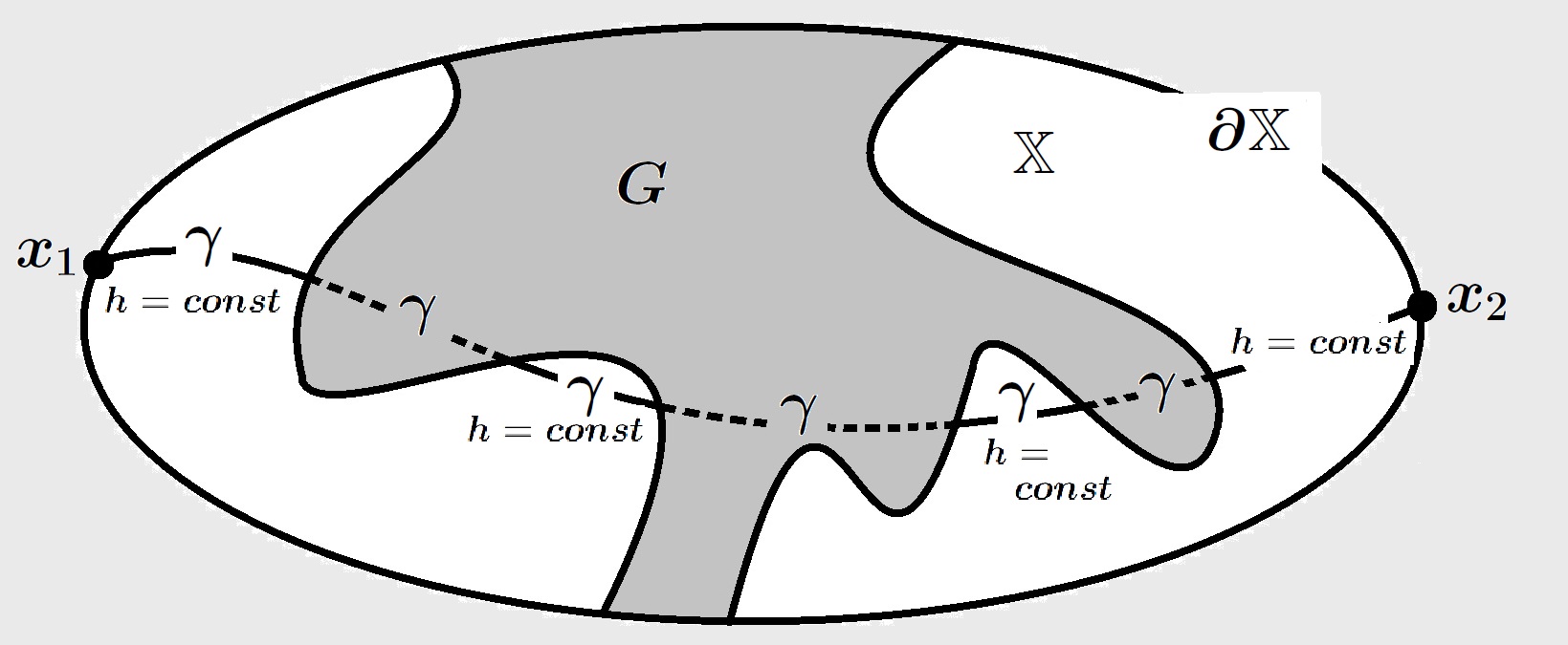
Figure 2. The set $f(G\cap\gamma)$ is an arc

Now, by Lemma 2.3 we have

$$\int_{f(\gamma{{}_{|_{\mathbb{G}}}})}\sqrt{\lvert\varphi\rvert}\,\lvert\textnormal{d}z\rvert\geqslant\int_{\gamma}\sqrt{\lvert\varphi\rvert}\,\lvert\textnormal{d}z\rvert$$

Therefore,

$$\int_{\gamma}\lvert\partial_{{}_{\mathsf{V}}}f\rvert\sqrt{\lvert\varphi\circ f\rvert}\cdot\chi_{{}_{\mathbb{G}}}\geqslant\int_{\gamma}\sqrt{\lvert\varphi\rvert}$$

Fubini’s ntegration formula (2.9) yields

(3.15) $$\int_{\mathbb{G}}\lvert\partial_{{}_{\mathsf{V}}}f\rvert\sqrt{\lvert\varphi\rvert}\sqrt{\lvert\varphi\circ f\rvert}\geqslant\int_{\mathbb{X}}\lvert\varphi\rvert$$

Combining (3.12) and (3.15), we obtain

(3.16) $$\int_{\mathbb{G}}\frac{\lvert\partial_{{}_{\mathsf{V}}}f\rvert^{2}}{J_{f}}\,\lvert\varphi\rvert\,\textnormal{d}z\geqslant\int_{\mathbb{X}}\lvert\varphi\rvert$$

This together with (3.10) and (3.11) gives

$$E_{\mathbb{X}}[H]-\mathcal{E}_{\mathbb{X}}[h]\geqslant 0\,,$$

as claimed. This also finishes the proof of Proposition 3.4. ∎

3.6. Uniqueness, proof of Theorem 1.8

Let $h$ and $H$ be Hopf-harmonic monotone mappings from $\overline{\mathbb{X}}$ onto $\overline{\mathbb{Y}}$ which coincides with $g$ on $\partial\mathbb{X}$. Therefore,

$$\begin{split}h_{z}\overline{h_{\bar{z}}}&=\varphi\qquad\textnormal{for some holomorphic }\varphi\\ H_{z}\overline{H_{\bar{z}}}&=\psi\qquad\textnormal{for some holomorphic }\psi\end{split}$$

We may assume that $\varphi\not\equiv 0\not\equiv\psi$. By Proposition 3.4 both mappings $h$ and $H$ minimize the Dirichlet energy subject to Sobolev monotone mapping in $\mathscr{M}_{g}(\overline{\mathbb{X}},\overline{\mathbb{Y}})$. Let us consider the subdomains of $\mathbb{X}$, $\mathbb{G}\stackrel{{\scriptstyle\textnormal{def}}}{{=\!\!=}}h^{-1}(\mathbb{Y})$ and $\mathbb{G}_{H}\stackrel{{\scriptstyle\textnormal{def}}}{{=\!\!=}}H^{-1}(\mathbb{Y})$. These are simply connected domains. In view of the partial harmonicity in (3.4), the mappings $h\colon\mathbb{G}\xrightarrow[]{{}_{\!\!\textnormal{onto\,\,}\!\!}}\mathbb{Y}$ and $H\colon\mathbb{G}_{H}\xrightarrow[]{{}_{\!\!\textnormal{onto\,\,}\!\!}}\mathbb{Y}$ are harmonic diffeomorphisms. Thus $f=H^{-1}\circ h\colon\mathbb{G}\xrightarrow[]{{}_{\!\!\textnormal{onto\,\,}\!\!}}\mathbb{G}_{H}$ is an orientation preserving diffeomorphism. We denote the inverse of $f$ by $g=f^{-1}=h^{-1}\circ H\colon\mathbb{G}_{H}\xrightarrow[]{{}_{\!\!\textnormal{onto\,\,}\!\!}}\mathbb{G}$. Fix a disk $\mathbb{D}\Subset\mathbb{G}_{H}$. There exists a sequence of diffeomorphisms $H_{k}\in\operatorname{Diff}_{g}(\overline{\mathbb{X}},\overline{\mathbb{Y}})$ converging to $H$ uniformly and in $\mathscr{W}^{1,2}(\mathbb{X},\mathbb{C})$. In analogy to $f$ and $g$ we define

$$f^{k}\stackrel{{\scriptstyle\textnormal{def}}}{{=\!\!=}}H_{k}^{-1}\circ h\colon\mathbb{G}\xrightarrow[]{{}_{\!\!\textnormal{onto\,\,}\!\!}}\mathbb{X}\quad\textnormal{ and }\quad g^{k}\stackrel{{\scriptstyle\textnormal{def}}}{{=\!\!=}}h^{-1}\circ H_{k}\colon\mathbb{X}\xrightarrow[]{{}_{\!\!\textnormal{onto\,\,}\!\!}}\mathbb{G}$$

Since $H_{k}\colon\overline{\mathbb{D}}\to\mathbb{Y}$ converge uniformly to $H\colon\mathbb{D}\to H(\overline{\mathbb{D}})$, where $H(\overline{\mathbb{D}})$ is a compact subset of $\mathbb{Y}$, there is a neighborhood $\mathbb{V}$ of $H(\overline{\mathbb{D}})$, compactly contained in $\mathbb{Y}$, such that $H_{k}(\overline{\mathbb{D}})\subset\mathbb{V}$ for all sufficiently large $k$, say for $k\geqslant k_{\circ}$. Since $\overline{\mathbb{V}}$ is compact in $\mathbb{Y}$ the set $\mathbb{F}\stackrel{{\scriptstyle\textnormal{def}}}{{=\!\!=}}h^{-1}(\overline{\mathbb{V}})$ is compact in $\mathbb{G}$. Then we note that

$$g^{k}(\overline{\mathbb{D}})=h^{-1}\big{(}H_{k}(\overline{\mathbb{D}})\big{)}\subset h^{-1}(\overline{\mathbb{V}})=\mathbb{F}\,.$$

Furthermore, $g^{k}$ converges uniformly to $g=h^{-1}\circ H\colon\overline{\mathbb{D}}\to h^{-1}\big{(}H(\overline{\mathbb{D}})\big{)}$. In view of (3.10), it follows that

(3.17) $$\begin{split}\mathcal{E}_{\mathbb{X}}[H_{k}]-\mathcal{E}_{\mathbb{X}}[h]&=4\int_{\mathbb{G}}\frac{\lvert\partial_{{}_{\mathsf{V}}}f^{k}\rvert^{2}}{J_{f^{k}}}\,\lvert\varphi\rvert\,\textnormal{d}z-4\,\int_{\mathbb{X}}\,\lvert\varphi\rvert\,\textnormal{d}z\\ &+4\int_{\mathbb{G}}\frac{(\,\lvert h_{z}\rvert\,-\,\lvert h_{\bar{z}}\rvert\,)^{2}\cdot\lvert f^{k}_{\bar{z}}\rvert^{2}}{J_{f^{k}}}\,\textnormal{d}z\,.\end{split}$$

Applying (3.16) with $f^{k}$ in place of $f$

$$\begin{split}\mathcal{E}_{\mathbb{X}}[H_{k}]-\mathcal{E}_{\mathbb{X}}[h]&\geqslant 4\int_{\mathbb{G}}\frac{(\,\lvert h_{z}\rvert\,-\,\lvert h_{\bar{z}}\rvert\,)^{2}\cdot\lvert f^{k}_{\bar{z}}\rvert^{2}}{J_{f^{k}}}\,\textnormal{d}z\\ &\geqslant 4\int_{\mathbb{F}}\frac{(\,\lvert h_{z}\rvert\,-\,\lvert h_{\bar{z}}\rvert\,)^{2}\cdot\lvert f^{k}_{\bar{z}}\rvert^{2}}{J_{f^{k}}}\,\textnormal{d}z\,.\end{split}$$

Since $h$ is an orientation-preserving diffeomorphism on $\mathbb{G}$, we have $\lvert h_{z}\rvert\,-\,\lvert h_{\bar{z}}\rvert\geqslant c>0$ for every $z\in\mathbb{F}\Subset\mathbb{G}$ and a constant $c=c(\mathbb{F})>0$

$$\begin{split}\mathcal{E}_{\mathbb{X}}[H_{k}]-\mathcal{E}_{\mathbb{X}}[h]&\geqslant 4c^{2}\int_{\mathbb{F}}\frac{\lvert f^{k}_{\bar{z}}\rvert^{2}}{J_{f^{k}}}\,\textnormal{d}z=4c^{2}\int_{f^{k}(\mathbb{F})}\lvert g^{k}_{\bar{w}}(w)\rvert^{2}\,\textnormal{d}w\\ &\geqslant 4c^{2}\int_{\mathbb{D}}\lvert g^{k}_{\bar{w}}(w)\rvert^{2}\,\textnormal{d}w\end{split}$$

Here we have made the substitution $z=g^{k}(w)$.

Letting $k\to\infty$ we find that $g^{k}_{\bar{w}}\to 0$ in $\mathscr{L}^{2}(\mathbb{D})$. Since $g^{k}\to g$ uniformly on $\mathbb{D}$, we see that $g_{\bar{w}}=0$ on $\mathbb{D}$. But $\mathbb{D}\Subset\mathbb{G}_{H}$ was arbitrary, so $g\colon\mathbb{G}_{H}\xrightarrow[]{{}_{\!\!\textnormal{onto\,\,}\!\!}}\mathbb{G}$ and $f=g^{-1}\colon\mathbb{G}\xrightarrow[]{{}_{\!\!\textnormal{onto\,\,}\!\!}}\mathbb{G}_{H}$ are conformal.

Next, using Lemma 3.3, we are going to show that $f(z)=z$. Here, the assumption that the part of $\partial\mathbb{Y}$ is convex is employed. By Lemma 3.3 we obtain that $\overline{h^{-1}(\mathbb{Y})}$ contains an open arc, $\Gamma\subset\partial\mathbb{X}$. Now, the conformal map $f\colon\mathbb{G}\xrightarrow[]{{}_{\!\!\textnormal{onto\,\,}\!\!}}\mathbb{G}_{H}$ extends continuously to $\Gamma$. Since $h(z)=H(z)$ on the boundary of $\mathbb{X}$, we have that $f(z)=z$ on $\Gamma$. Finally, we appeal to a general fact that two holomorphic functions in $\mathbb{G}$, continuous on $\overline{\mathbb{G}}$, are the same if they coincide on an arc of $\partial\mathbb{G}$. Therefore, $f(z)=z$ in $\mathbb{G}$, which means that $h(z)=H(z)$ for all $z\in\mathbb{G}$. Now, the holomorphic functions $\varphi=h_{z}\overline{h_{\bar{z}}}$ and $\psi=H_{z}\overline{H_{\bar{z}}}$ coincide in $\mathbb{G}$ and so

$$\varphi(z)=\psi(z)\qquad\textnormal{ for all }z\in\mathbb{X}\,.$$

What remains is to argue that $h=H$ in $\mathbb{X}\setminus\mathbb{G}$. Note that $h$ and $H$ have the same vertical trajectories (because $\varphi\equiv\psi$). By Lemma 2.6 they are constant on every connected component (arc) of every every vertical trajectory. Since $h$ and $H$ coincide on the endpoints of these arcs, we conclude that $h\equiv H$ on $\mathbb{X}\setminus\mathbb{G}$, which completes the proof.

3.7. Proof of Theorem 1.3

Since every $\mathscr{C}^{2}$-regular domain $\mathbb{Y}$ is a somewhere convex Lipschitz domain Theorem 1.3 follows from Theorem 1.5 and Theorem 1.8.

4. Examples

We will now demonstrate, by way of illustration, of how the above results work for monotone Hopf harmonics $\,h:\mathbb{X}\xrightarrow[]{{}_{\!\!\textnormal{onto\,\,}\!\!}}\mathbb{Y}\,$ between domains with certain symmetries. In our first example the target $\mathbb{Y}\subset\mathbb{C}$ has the butterfly shape, with exactly one non-convex boundary point, see Figure 3.

Example 4.1.

We use the polar coordinates for $z$ in the closed unit disk $\overline{\mathbb{D}}$, $z=\rho e^{i\theta}$, $0\leqslant\rho\leqslant 1$ and $0\leqslant\theta<2\pi$. Define $h\colon\overline{\mathbb{D}}\to\mathbb{C}$ by the rule:

$$\begin{split}h(\rho e^{i\theta})&=2\rho\left[\sqrt{\rho}\sin(\nicefrac{{3}}{{2}}\,\theta)+i\sin\theta\right]=z-\bar{z}-i\left[z^{\nicefrac{{3}}{{2}}}-\bar{z}^{\nicefrac{{3}}{{2}}}\right].\end{split}$$

This mapping is Lipschitz continuous with

(4.1) $$h_{z}=1-\nicefrac{{3}}{{2}}\,i\sqrt{z},\qquad h_{\bar{z}}=-1+\nicefrac{{3}}{{2}}\,i\sqrt{\bar{z}}.$$

Moreover, its Hopf differential is holomorphic

(4.2) $$h_{z}\overline{h_{\bar{z}}}=-\nicefrac{{1}}{{4}}\,\left(4+9z\right).$$

Thus $h$ solves the Hopf-Laplace equation $\frac{\partial}{\partial\bar{z}}\left(h_{z}\overline{h_{\bar{z}}}\right)=0$. Concerning topological behavior, the ray $\mathbb{I}=\{z\colon\operatorname{Im}z=0\mbox{ and }0\leqslant\operatorname{Re}z\leqslant 1\}$ is squeezed into the origin, which is a boundary point of $\mathbb{Y}$. Outside of the ray, the mapping $h$ is homeomorphism and it takes $\mathbb{D}\setminus\mathbb{I}$ as a harmonic diffeomorphism onto the domain $\mathbb{Y}$ , see Figure 3.

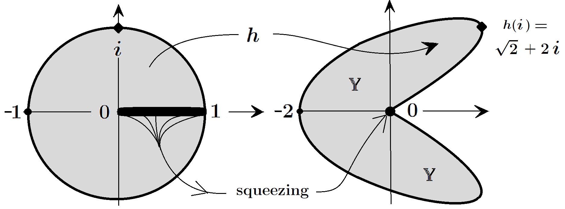
Figure 3. A horizontal segment is squeezed into a point where $\,\mathbb{Y}\,$ fails to be convex

Example 4.2.

In our second example the target $\mathbb{Y}\subset\mathbb{C}$ is a semi-annulus in which the inner semi-circular boundary arc consists of non-convex points. Consider a horizontal strip

$$\,\mathcal{S}=\mathbb{R}\times\left[-\frac{\pi}{2},\frac{\pi}{2}\right]\;=\mathcal{S}_{-}\cup\mathcal{S}_{+}\;,\;\;\textnormal{where}\;$$

$$\mathcal{S}_{-}\stackrel{{\scriptstyle\textnormal{def}}}{{=\!\!=}}\left(-\infty,0\,\right]\times\left[-\frac{\pi}{2},\frac{\pi}{2}\right]\;\;\textnormal{and}\;\;\mathcal{S}_{+}\stackrel{{\scriptstyle\textnormal{def}}}{{=\!\!=}}\left[\,0,+\infty\,\right)\times\left[-\frac{\pi}{2},\frac{\pi}{2}\right]$$

We define a mapping $\,h=u+i\,v:\mathcal{S}\rightarrow\mathbb{C}\,$ by the rule

$$h(x,y)=\begin{cases}e^{iy}\cosh\,x\qquad&\textnormal{\;if }\;0\leqslant x<+\infty\\ e^{iy}\qquad&\textnormal{\;if}\;-\infty<x\leqslant 0\end{cases}$$

It is straightforward to verify that $\,h\,$ is a $\,\mathscr{C}^{1,1}\,$-smooth monotone Hopf harmonic, but not $\mathscr{C}^{2}\,$ -smooth. In fact, we have $\,h_{z}\,\overline{h_{\overline{z}}}\,\equiv-\frac{1}{4}\,$ in the entire strip. This map takes the vertical cross sections of $\,\mathcal{S}_{+}\,$ onto concentric semicircles $\,\mathcal{C}_{\rho}\stackrel{{\scriptstyle\textnormal{def}}}{{=\!\!=}}\{(u,v):\,u^{2}+v^{2}=\rho^{2}\;,\;u\geqslant 0\,\}\,$ , $\,1\leqslant\rho<\infty\,$, see Figure 4. On the other hand, in $\,\mathcal{S}_{-}\,$ each half line $\,\{(x,y);\;-\infty<x\leqslant 0\,\}$, parametrized by $\,y\in\left[-\frac{\pi}{2},\frac{\pi}{2}\right]\,$, is squeezed into a point $\,e^{iy}\,\in\mathcal{C}_{1}\,$. Now consider a rectangular box $\,\mathbb{X}=\mathbb{X}_{-}\cup\mathbb{X}_{+}\,$, where

$$\,\mathbb{X}_{-}\stackrel{{\scriptstyle\textnormal{def}}}{{=\!\!=}}\left\{(x,y)\colon\,-\ell<x<0\;,\;-\frac{\pi}{2}<y<\frac{\pi}{2}\,\right\}\,$$

$$\,\mathbb{X}_{+}\stackrel{{\scriptstyle\textnormal{def}}}{{=\!\!=}}\left\{(x,y)\colon\,0\leqslant x<T\;,\;-\frac{\pi}{2}<y<\frac{\pi}{2}\,\right\}\;$$

Our monotone Hopf harmonic map $\,h\,$ takes $\,\mathbb{X}\,$ onto a semi-annulus $\,\mathbb{Y}\stackrel{{\scriptstyle\textnormal{def}}}{{=\!\!=}}\{(u,v)\,;\,1<\sqrt{u^{2}+v^{2}}<\cosh T\;,\;u>0\,\}\,$, so $\,h^{-1}(\mathbb{Y})=\mathbb{X}_{+}\,$.

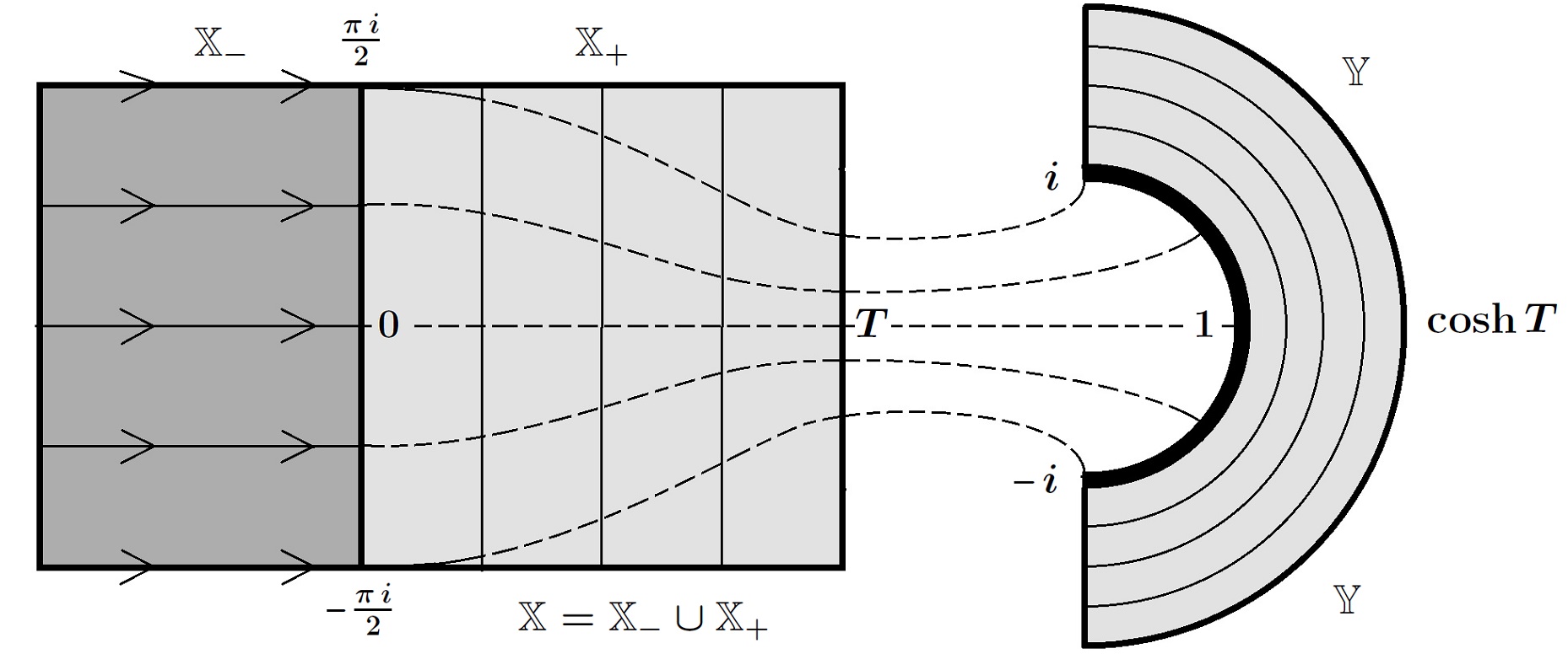
Figure 4. Points in $\mathbb{X}_{-}\,$ are projected onto the common boundary $\,\partial\mathbb{X}_{-}\cap\partial\mathbb{X}_{+}\,$, and then transformed into the semicircular boundary arc of $\,\mathbb{Y}\,$, exactly where it fails to be convex.

5. 4-leaf clovers

In our third example the target $\mathbb{Y}$ has a 4-leaf clovers shape.

5.1. Circular and Elliptical Clovers

The reference configuration $\,\mathbb{X}\subset\mathbb{C}\simeq\mathbb{R}^{2}\,$ will be a union of four disks of radius 1 centered at the points $\,1,i,-1,-i\,$. Call $\,\mathbb{X}\,$ a circular 4-leaf clover. Thus the boundary of $\,\mathbb{X}\,$ consists of four semicircular arcs, which we write as $\,\partial\mathbb{X}=\mathbf{\Gamma}_{2}\,\cup\,\mathbf{\Gamma}_{2i}\,\cup\,\mathbf{\Gamma}_{-2}\,\cup\,\mathbf{\Gamma}_{-2i}\,$. Each complex subscript here designates middle point of the arc, see Figure 5.

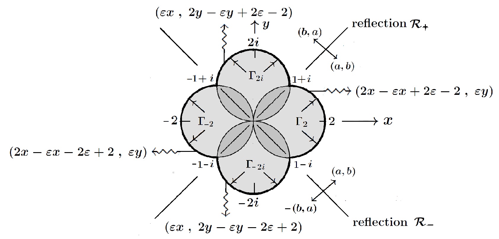
Figure 5. 4-leaf circular clover and a piece-wise affine boundary data

The target domain $\,\mathbb{Y}\subset\mathbb{C}\simeq\mathbb{R}^{2}\,$ is a union of four ellipses obtained from the disks via affine transformations. We shall call it elliptical 4-leaf clover, see Figure 6.

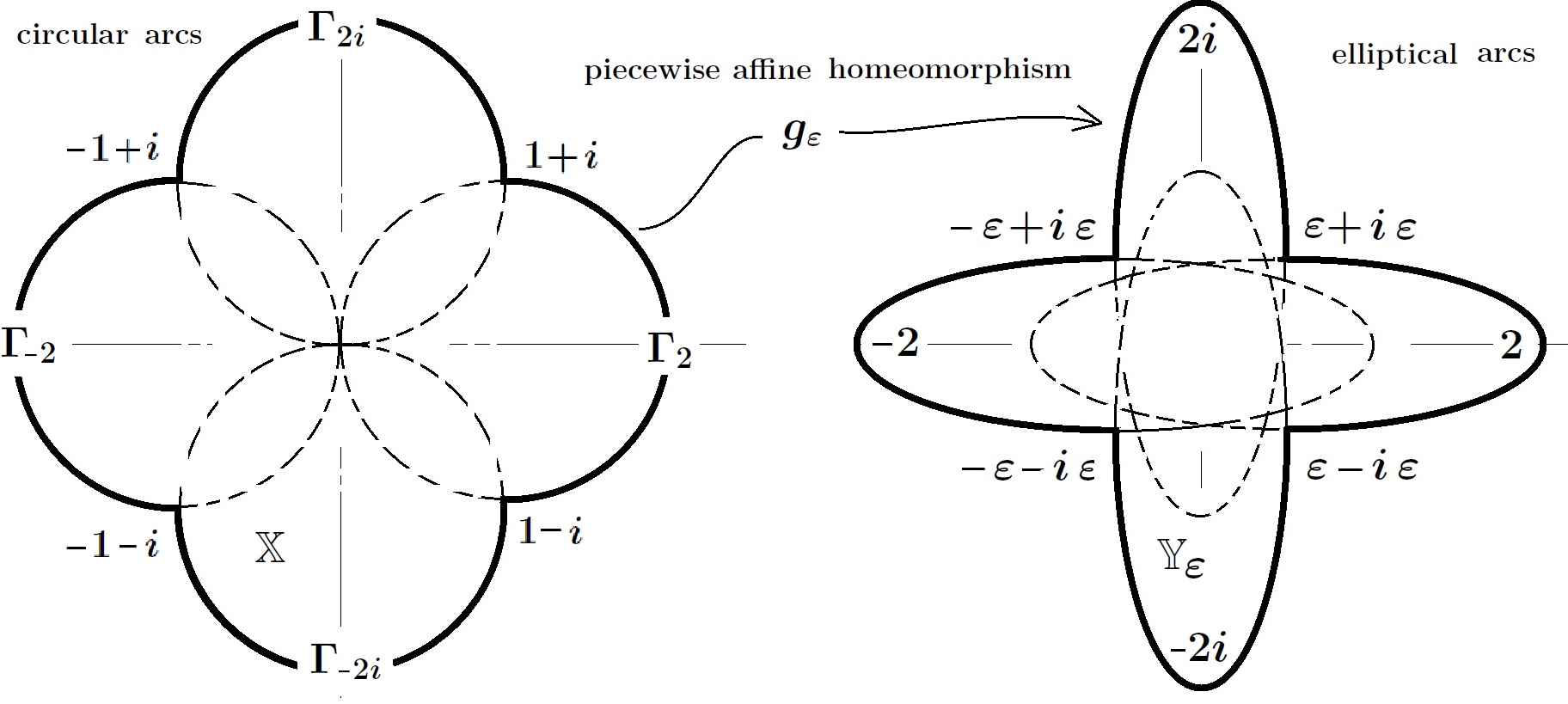
Figure 6. The boundary of the elliptical clover

The boundary of $\,\mathbb{Y}\,$ consists of four elliptical arcs, $\,\partial\mathbb{Y}\stackrel{{\scriptstyle\textnormal{def}}}{{=\!\!=}}g(\partial\mathbb{X})\stackrel{{\scriptstyle\textnormal{def}}}{{=\!\!=}}g(\mathbf{\Gamma}_{2})\,\cup\,g(\mathbf{\Gamma}_{2i})\,\cup\,g(\mathbf{\Gamma}_{-2})\,\cup\,g(\mathbf{\Gamma}_{-2i})\,$, where $\,g:\partial\mathbb{X}\xrightarrow[]{{}_{\!\!\textnormal{onto\,\,}\!\!}}\partial\mathbb{Y}\,$ is a piecewise affine map defined by the rule:

$$g(x,y)=g_{\varepsilon}(x,y)=\begin{cases}(2x-\varepsilon x+2\varepsilon-2\;,\;\varepsilon y)\;,\;\textnormal{for}\;(x,y)\in\mathbf{\Gamma}_{2}\;\\ (\varepsilon x\;,\;2y-\varepsilon y+2\varepsilon-2)\;,\;\textnormal{for}\;(x,y)\in\mathbf{\Gamma}_{2i}\;\\ (2x-\varepsilon x-2\varepsilon+2\;,\;\varepsilon y)\;,\;\textnormal{for}\;(x,y)\in\mathbf{\Gamma}_{-2}\;\\ (\varepsilon x\;,\;2y-\varepsilon y-2\varepsilon+2)\;,\;\textnormal{for}\;(x,y)\in\mathbf{\Gamma}_{-2i}\;\end{cases}$$

Here $\,0\leqslant\varepsilon\leqslant 1\,$ is a parameter to be chosen and fixed later on. For now, the elliptical 4-leaf clover actually depends on $\,\varepsilon\,$, which we indicate by writing $\,\mathbb{Y}=\mathbb{Y}_{\varepsilon}\,$ when clarity requires it.

5.2. Harmonic Extension $\,G=G_{\varepsilon}\,$

Except for $\,\varepsilon=0\,$, the boundary map $\,g:\partial\mathbb{X}\xrightarrow[]{{}_{\!\!\textnormal{onto\,\,}\!\!}}\partial\mathbb{Y}\,$ is a homeomorphism. We see that $\,g_{1}(x,y)=(x,y)\,$, so $\,\mathbb{Y}\,=\mathbb{X}\,$. In this case the harmonic extension of $\,g_{1}\,$ is the identity on $\,\mathbb{X}\,$ as well. As one may have expected, when $\,\varepsilon\,$ drops below 1, but not too far (say $\,\varepsilon\in[\varepsilon_{\sharp},1]\,$ for some $\,0<\varepsilon_{\sharp}\leqslant 1$), the harmonic extension, denoted by $\,G=G_{\varepsilon}:\overline{\mathbb{X}}\xrightarrow[]{{}_{\!\!\textnormal{into\,\,}\!\!}}\mathbb{R}^{2}\,$ of the boundary data $\,g_{\varepsilon}:\partial\mathbb{X}\xrightarrow[]{{}_{\!\!\textnormal{onto\,\,}\!\!}}\partial\mathbb{Y}_{\varepsilon}\,$ remains a diffeomorphism of $\,\mathbb{X}\xrightarrow[]{{}_{\!\!\textnormal{onto\,\,}\!\!}}\mathbb{Y}_{\varepsilon}\,$, see Figure 7.

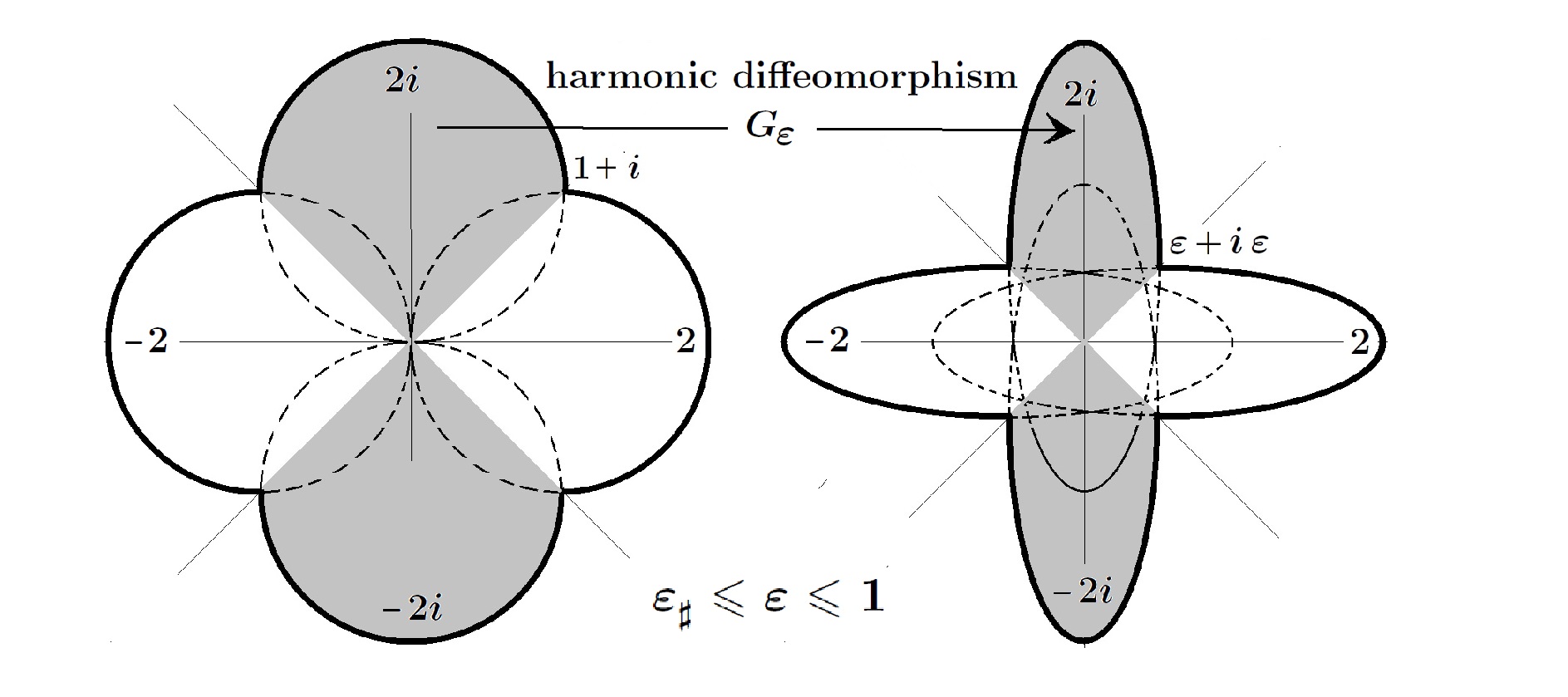
Figure 7. Circular clover and its diffeomorphic image by the harmonic extension of the boundary data

5.3. The Limit Case

Let us take a quick look at the limit of harmonic extensions as $\,\varepsilon\searrow 0\,$.

In case $\,\varepsilon=0\,$ the 4-leaf clover degenerates to a cross of coordinate segments, see Figure 8.

$$g_{{}_{0}}(x,y)=\begin{cases}(2x-2\;,\;0)\;,\;\textnormal{for}\;(x,y)\in\mathbf{\Gamma}_{2}\;\\ (0\;,\;2y-2)\;,\;\textnormal{for}\;(x,y)\in\mathbf{\Gamma}_{2i}\;\\ (2x+2\;,\;0)\;,\;\textnormal{for}\;(x,y)\in\mathbf{\Gamma}_{-2}\;\\ (0\;,\;2y+2)\;,\;\textnormal{for}\;(x,y)\in\mathbf{\Gamma}_{-2i}\;\end{cases}$$

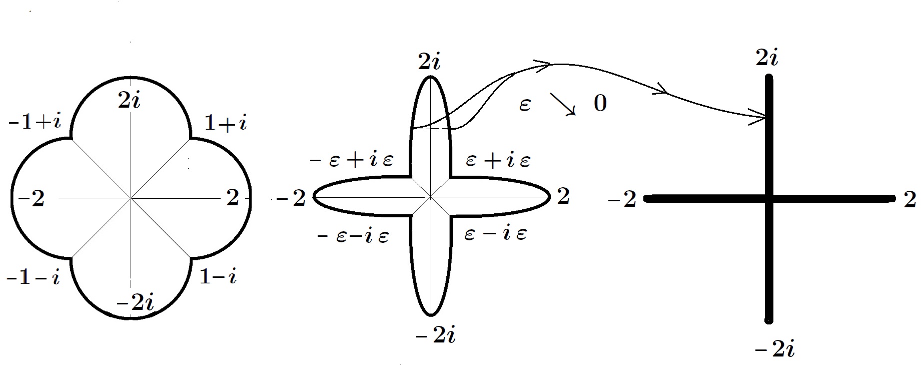
Figure 8. The uniform limit of the images of the boundary homeomorphisms degenerates to a cross of straight segments.

We always have the inclusion $\,G_{\varepsilon}(\overline{\mathbb{X}})\,\supseteq\overline{\mathbb{Y}_{\varepsilon}}\,$; just because of continuity of $\,G_{\varepsilon}\,$. However, if $\,\varepsilon$ is small enough, we have even strict inclusion $\,G_{\varepsilon}(\overline{\mathbb{X}})\,\varsupsetneq\overline{\mathbb{Y}_{\varepsilon}}\,$. Indeed, suppose that, on the contrary, there is a sequence $\,\varepsilon_{n}\searrow 0\,$ for which $\,G_{\varepsilon_{n}}(\overline{\mathbb{X}})\,\subset\overline{\mathbb{Y}_{\varepsilon_{n}}}\,$. The boundary homeomorphisms $\;g_{\varepsilon_{n}}:\,\partial\mathbb{X}\xrightarrow[]{{}_{\!\!\textnormal{onto\,\,}\!\!}}\partial\mathbb{Y}_{\varepsilon_{n}}\,$ converge uniformly to $\;g_{{}_{0}}:\,\partial\mathbb{X}\xrightarrow[]{{}_{\!\!\textnormal{onto\,\,}\!\!}}\partial\mathbb{Y}_{0}\,$. By the maximum/minimum principle it follows that $\,G_{\varepsilon_{n}}:\overline{\mathbb{X}}\xrightarrow[]{{}_{\!\!\textnormal{onto\,\,}\!\!}}\overline{\mathbb{Y}_{\varepsilon}}\,$ converge uniformly to a harmonic map $\,G_{0}\stackrel{{\scriptstyle\textnormal{def}}}{{=\!\!=}}u+iv\,$ whose image $\,G_{0}(\overline{\mathbb{X}})\,$ degenerates to a cross of straight line segments, see Figure 8. Thus $\,u\cdot v\equiv 0\,$ on $\,\overline{\mathbb{X}}\,$. This is possible only when $\,u\equiv 0\,$ or $\,v\equiv 0\,$, by the unique continuation property of harmonic functions, which is a contradiction.

5.4. Critical Parameter $\,\varepsilon_{\sharp}\;$

We just have shown that there is so-called critical parameter $\,0<\varepsilon_{\sharp}\leqslant 1\,$ such that: whenever $\,\varepsilon\,$ drops below $\,\varepsilon_{\sharp}\,$, the harmonic extension $\,G_{\varepsilon}:\overline{\mathbb{X}}\rightarrow\mathbb{R}^{2}\,$ of the boundary homeomorphism $\,g_{\varepsilon}:\partial\mathbb{X}\xrightarrow[]{{}_{\!\!\textnormal{onto\,\,}\!\!}}\partial\mathbb{Y}_{\varepsilon}\,$ takes part of $\,\mathbb{X}\,$ outside $\,\overline{\mathbb{Y}_{\sharp}}\,$, as in Figure 9. Overlapping becomes inevitable.

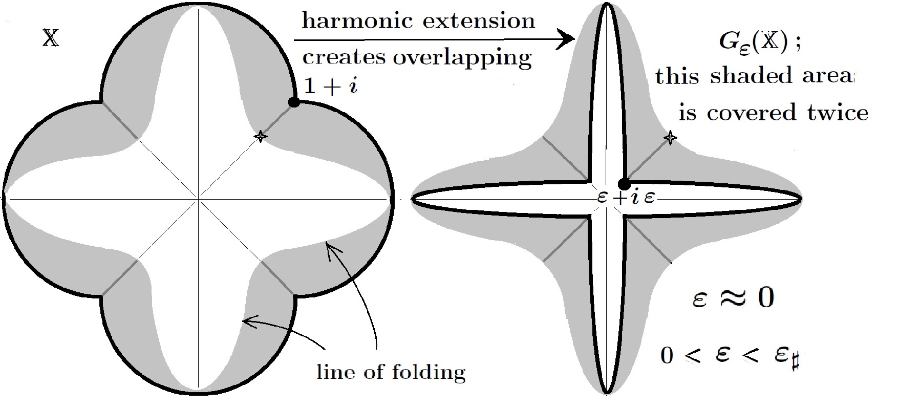
Figure 9. This hand made sketch may not be accurate regarding the actual lines of folding.

In the mathematical models of Nonlinear Elasticity the overlapping is ruled out by the principle of non interpenetration of matter. We just find ourselves forced to place topological restrictions on the mappings in question for minimizing the Dirichlet energy. Monotone Hopf harmonics turn out to be right solution; for, no overlapping may occur. As we shall illustrate in this example, monotone energy-minimal deformations will squeeze certain line fragments of $\,\mathbb{X}\,$ (emanating from $\,\partial\mathbb{X}\,$) into non convex points of $\,\partial\mathbb{Y}\,$. Nevertheless Hopf harmonics, being limits of Sobolev homeomorphisms, should take legitimate place in NE.

5.5. Below the Critical Parameter

This is the case $\,0<\varepsilon<\varepsilon_{\sharp}\,$ when harmonic extensions fail.

From now on, we choose and fix a parameter $\,0<\varepsilon<\varepsilon_{\sharp}\,$, so the harmonic extension $\,G_{\varepsilon}:\mathbb{X}\xrightarrow[]{{}_{\!\!\textnormal{into\,\,}\!\!}}\mathbb{R}^{2}\,$ is ruled out by models of NE.

5.6. Monotone Hopf Harmonic map $\,H=H_{\varepsilon}$

Advantageously, Theorem 1.5, provides us with a unique monotone Hopf-harmonic map, denoted by $\,H=H_{\varepsilon}:\overline{\mathbb{X}}\xrightarrow[]{{}_{\!\!\textnormal{onto\,\,}\!\!}}\overline{\mathbb{Y}}=\overline{\mathbb{Y}_{\varepsilon}}\,$, of class $\,\mathscr{C}(\overline{\mathbb{X}},\overline{\mathbb{Y}_{\varepsilon}})\cap\mathscr{W}^{1,2}(\mathbb{X},\mathbb{Y}_{\varepsilon})\,$, which agrees with $\,g=g_{\varepsilon}\,$ on $\,\partial\mathbb{X}\,$. Furthermore, $\,H\,$ is a harmonic diffeomorphism from $\,H^{-1}(\mathbb{Y})\,$ onto $\,\mathbb{Y}\,$. Actually, among all monotone Sobolev mappings with prescribed boundary data $\,g:\partial\mathbb{X}\xrightarrow[]{{}_{\!\!\textnormal{onto\,\,}\!\!}}\partial\mathbb{Y}=\partial\mathbb{Y}_{\varepsilon}\,$, the map $\,H\,$ is a unique one with smallest Dirichlet energy, see Proposition 3.4. Our choice of 4-leaf clovers comes from the fact that the symmetries of $\,\mathbb{X}\,$ and $\,\mathbb{Y}\,$ about the coordinate axes $\,y=0\,,\,x=0\,$ and the diagonal lines $\,y=x\,,\,y=-x\,$ will help us to locate the squeezing fragments of $\,\mathbb{X}\,$.

We start with the observation that the boundary data is also symmetric about these lines; in symbols,

(5.1) $$\begin{split}&g\circ\mathcal{T}_{\pm}=\mathcal{T}_{\pm}\circ g\;,\;\;\textnormal{where}\;\;\mathcal{T}_{\pm}(a,b)\stackrel{{\scriptstyle\textnormal{def}}}{{=\!\!=}}\pm(a,-b)\,\;\;\textnormal{(respectively)}\\ &g\circ\mathcal{R}_{\pm}=\mathcal{R}_{\pm}\circ g\;,\;\;\textnormal{where}\;\;\mathcal{R}_{\pm}(a,b)\stackrel{{\scriptstyle\textnormal{def}}}{{=\!\!=}}\pm(b,a)\,\;\;\textnormal{(respectively)}\end{split}$$

The above commutation rules can easily be verified; make use of the explicit formulas conveniently provided in Figure 5 for this purpose. Using complex variable $\,z=x+iy\,$, the reflections $\,\mathcal{T}_{\pm}:\mathbb{C}\xrightarrow[]{{}_{\!\!\textnormal{onto\,\,}\!\!}}\mathbb{C}\,$ and $\,\mathcal{R}_{\pm}:\mathbb{C}\xrightarrow[]{{}_{\!\!\textnormal{onto\,\,}\!\!}}\mathbb{C}\,$ read as: $\,\mathcal{T}_{\pm}(z)=\pm\overline{z}\,$ and $\,\mathcal{R}_{\pm}(z)=\pm i\overline{z}\,$. In particular, the boundary data is also invariant under rotation by right angle; namely, $\,(\mathcal{T}_{\pm}\circ\mathcal{R}_{\pm})(z)=iz\,$. The observed symmetries carry over to the Hopf harmonic map $\,H:\overline{\mathbb{X}}\xrightarrow[]{{}_{\!\!\textnormal{onto\,\,}\!\!}}\overline{\mathbb{Y}}\,$ as well; precisely,

(5.2) $$\begin{split}&H\circ\mathcal{T}_{\pm}=\mathcal{T}_{\pm}\circ H\;:\;\overline{\mathbb{X}}\xrightarrow[]{{}_{\!\!\textnormal{onto\,\,}\!\!}}\overline{\mathbb{Y}}\;\;\textnormal{(respectively)}\\ &H\circ\mathcal{R}_{\pm}=\mathcal{R}_{\pm}\circ H\;:\;\overline{\mathbb{X}}\xrightarrow[]{{}_{\!\!\textnormal{onto\,\,}\!\!}}\overline{\mathbb{Y}}\;\;\textnormal{(respectively)}\end{split}$$

To see this examine, in addition to $\,H:\overline{\mathbb{X}}\xrightarrow[]{{}_{\!\!\textnormal{onto\,\,}\!\!}}\overline{\mathbb{Y}}\,$, four monotone mappings;

(5.3) $$\begin{split}&\,\mathbf{T}^{\pm}\stackrel{{\scriptstyle\textnormal{def}}}{{=\!\!=}}\mathcal{T}_{\pm}\circ H\circ\mathcal{T}_{\pm}\,:\,\overline{\mathbb{X}}\xrightarrow[]{{}_{\!\!\textnormal{onto\,\,}\!\!}}\overline{\mathbb{Y}}\,\\ &\,\mathbf{R}^{\pm}\stackrel{{\scriptstyle\textnormal{def}}}{{=\!\!=}}\mathcal{R}_{\pm}\circ H\circ\mathcal{R}_{\pm}\,:\,\overline{\mathbb{X}}\xrightarrow[]{{}_{\!\!\textnormal{onto\,\,}\!\!}}\overline{\mathbb{Y}}\,\end{split}$$

They all share the same boundary data $\,g:\partial\mathbb{X}\xrightarrow[]{{}_{\!\!\textnormal{onto\,\,}\!\!}}\partial\mathbb{Y}=\partial\mathbb{Y}_{\varepsilon}\,$. Let their Hopf products be denoted by:

(5.4) $$\begin{split}&\zeta(z)=H_{z}(z)\cdot\overline{H_{\overline{z}}(z)}\;\;,\;\;\textnormal{for}\;\;z\in\mathbb{X}\\ &\;\psi^{\pm}(z)=\mathbf{T}^{\pm}_{z}(z)\cdot\overline{\mathbf{T}^{\pm}_{\overline{z}}(z)}\;\\ &\;\;\phi^{\pm}(z)=\mathbf{R}^{\pm}_{z}(z)\cdot\overline{\mathbf{R}^{\pm}_{\overline{z}}(z)}\end{split}$$

These functions are holomorphic in $\,\mathbb{X}\,$. In fact, we have the following formulas for the Hopf products

$$\psi^{\pm}(z)\;=\;\overline{\zeta(\pm\overline{z})}\;,\;\;\;\textnormal{and}\;\;\phi^{\pm}(z)\;=\;-\overline{\zeta(\pm i\overline{z})}\;,\;\;\textnormal{respectively.}$$

Since $\,\zeta\,$ is holomorphic in $\,\mathbb{X}\,$, so are the Hopf products $\;\psi^{\pm}\,$ and $\,\phi^{\pm}\,$. Now comes the uniqueness statement in Theorem 1.5. It tells us that all of the above five monotone mappings are the same. We just have established the commutation rules (5.2), whence it is readily inferred that $\,H\,$ takes points in each of the four lines of symmetry into the same line.

5.7. Straight Line Segments of Symmetry

To make it more precise, there are four straight line segments to be considered (sections of $\,\overline{\mathbb{X}}\,$ along the symmetry lines).

$$\begin{cases}\mathbf{A}=\{(x,0)\,;\,\;-2\leqslant x\leqslant 2\,\}\;\;,\;\;\textnormal{thus}\;\;\;H:\mathbf{A}\xrightarrow[]{{}_{\!\!\textnormal{onto\,\,}\!\!}}\mathbf{A}\\ \mathbf{B}=\{(x,x)\,;\,\;-1\leqslant x\leqslant 1\,\}\;\;,\;\;\textnormal{thus}\;\;\;H:\mathbf{B}\xrightarrow[]{{}_{\!\!\textnormal{onto\,\,}\!\!}}\varepsilon\mathbf{B}\\ \mathbf{C}=\{(0,y)\,;\,\;\,-2\leqslant y\leqslant 2\,\}\;\;,\;\;\textnormal{thus}\;\;\;H:\mathbf{C}\xrightarrow[]{{}_{\!\!\textnormal{onto\,\,}\!\!}}\mathbf{C}\\ \mathbf{A}=\{(x,-x)\,;\,-1\leqslant x\leqslant 1\}\;,\;\;\textnormal{thus}\;\;H:\mathbf{D}\xrightarrow[]{{}_{\!\!\textnormal{onto\,\,}\!\!}}\varepsilon\mathbf{D}\end{cases}$$

In particular, $\,H(0)=0\,$.

5.8. Janiszewski Theorem

Our nearest goal is to show that:

Lemma 5.1.

All the above four mappings are monotone on their segments of definition.

Proof.

The proof will only be given for the mapping $\,H:\mathbf{A}\xrightarrow[]{{}_{\!\!\textnormal{onto\,\,}\!\!}}\mathbf{A}$; the other cases can be treated in much the same way. The key ingredient is the topological theorem of Z. Janiszewski [21] (1913).

Definition 5.2.

With reference to K. Kuratowski’ book ([26], Topology Vol. II, page 505), the Janiszewski space is a locally connected continuum having the following property:

If $\,\mathcal{C}_{+}\,$ and $\,\mathcal{C}_{-}\,$ are two continua whose intersection $\,\mathcal{C}_{+}\cap\mathcal{C}_{-}\,$ is not connected, the union $\,\mathcal{C}_{+}\cup\mathcal{C}_{-}\,$ is a cut of the space (its complement is disconnected).

The sphere $\,\mathbb{S}^{2}\,$ is a Janiszewski space

see [26], Ch. X, page 506.

Figure 10. Janiszewski continua with two complementary components

Now choose and fix a point in the target space, say $\,q\in H(\mathbf{A})=\mathbf{A}\,$. Since $\,H:\overline{\mathbb{X}}\xrightarrow[]{{}_{\!\!\textnormal{onto\,\,}\!\!}}\overline{\mathbb{Y}}\,$ is monotone, its preimage $\,\mathcal{C}\stackrel{{\scriptstyle\textnormal{def}}}{{=\!\!=}}\{z\in\overline{\mathbb{X}}:H(z)=q\,\}$ is a continuum. Our aim is to show that $\,\mathcal{C}\cap\mathbf{A}\,$ is connected. For this, we first observe (quite a general fact about monotone mappings) that $\,\mathcal{C}\subset\mathbb{R}^{2}\,$ is not a cut of $\,\mathbb{R}^{2}\,$, meaning that its complement is connected. Indeed, we have

$$\mathbb{R}^{2}\setminus\mathcal{C}=(\mathbb{R}^{2}\setminus\overline{\mathbb{X}})\cup(\overline{\mathbb{X}}\setminus\mathcal{C}))\;,\;\;\textnormal{because}\;\;\mathcal{C}\subset\overline{\mathbb{X}}\,$$

Both terms in this union are connected; the first by obvious reasons, the second is just a primage under $\,H:\overline{\mathbb{X}}\xrightarrow[]{{}_{\!\!\textnormal{onto\,\,}\!\!}}\overline{\mathbb{Y}}\,$ of the connected set $\,\overline{\mathbb{Y}}\setminus\{q\}\,$. We need only verify that the intersection of those terms is not empty. But this is immediate from the formula

$$(\mathbb{R}^{2}\setminus\overline{\mathbb{X}})\cap(\overline{\mathbb{X}}\setminus\mathcal{C})\;=\;\partial\mathbb{X}\setminus\mathcal{C}\not=\emptyset$$

We are now in a position to appeal to Janiszewski Theorem.

For this, note that the above-mentioned symmetry of $\,H\,$ yields the respective symmetry of $\,\mathcal{C}\,$. Specifically, $\,z\in\mathcal{C}\;\;\rightleftarrows\;\;\bar{z}\in\mathcal{C}\,$. Then $\,\mathcal{C}\,$ can be decomposed in accordance with sign of $\,\Im m\,z\,$ as follows: $\,\mathcal{C}=\mathcal{C}_{+}\cup\,\mathcal{C}_{-}\,$, where

$$\mathcal{C}_{+}=\{z\in\mathcal{C}:\;\Im m\,z\geqslant 0\,\}\;\;\textnormal{ and}\;\;\mathcal{C}_{-}=\{z\in\mathcal{C}:\;\Im m\,z\leqslant 0\,\}$$

It is readily seen that both $\,\mathcal{C}_{+}\,$ and $\,\mathcal{C}_{-}\,$ are continua, and

$$\mathcal{C}\cap\mathbf{A}=\mathcal{C}_{+}\cap\mathcal{C}_{-}\;\;\;$$

Since $\,\mathcal{C}\,$ is not a cut of $\,\mathbb{R}^{2}\,$, by Janiszewski’s Theorem, the intersection $\,\mathcal{C}_{+}\cap\,\mathcal{C}_{-}\,$ must be connected, completing the proof of Lemma 5.1. ∎

5.9. Segments of Squeezing

The next step in our discussion is to look at the pre-images of the four points $\,\pm\varepsilon\pm i\varepsilon\,$ (exactly where $\,\partial\mathbb{Y}_{\varepsilon}\,$ fails to be convex) under the monotone mappings $\,H:\mathbf{B}\xrightarrow[]{{}_{\!\!\textnormal{onto\,\,}\!\!}}\varepsilon\mathbf{B}\,$ and $\,H:\mathbf{D}\xrightarrow[]{{}_{\!\!\textnormal{onto\,\,}\!\!}}\varepsilon\mathbf{D}\,$, respectively. These pre-images, being connected, must be straight line segments in $\,\mathbf{B}\,$ and $\,\mathbf{D}\,$ with endpoints at $\,\pm 1\pm i\,$, respectively. They do not pass through the origin, because $\,H(0)=0\,$. They have the same length (possibly zero) because of the rotational symmetry $\,H(iz)=iH(z)\,$. Let us denote these segments by,

$$\mathbf{B}^{+}=\{t+it\,;\,\rho\leqslant t\leqslant 1\,\}\;\;,\;\;\mathbf{B}^{-}=\{-t-it\,;\,\rho\leqslant t\leqslant 1\,\}$$

$$\mathbf{D}^{+}=\{t-it\,;\,\rho\leqslant t\leqslant 1\,\}\;\;,\;\;\mathbf{D}^{-}=\{-t+it\,;\,\rho\leqslant t\leqslant 1\,\}$$

Remark 5.3.

Note that at this stage of our arguments one cannot claim yet that $\,\mathbf{B}^{\pm}\,$ and $\,\mathbf{D}^{\pm}\,$ are the only collapsing sets, though it will turn out to be true.

5.10. Outside the Cracks

We now remove the collapsing segments $\,\mathbf{B}^{\pm}\,$ and $\,\mathbf{D}^{\pm}\,$ from $\,\mathbb{X}\,$ (interpreting them as cracks in $\,\mathbb{X}\,$ that are squeezed to the boundary points at which $\,\partial\mathbb{Y}\,$ fails to be convex),

(5.5) $$\mathbb{X}_{\divideontimes}\stackrel{{\scriptstyle\textnormal{def}}}{{=\!\!=}}\mathbb{X}\setminus(\mathbf{B}^{+}\cup\mathbf{B}^{-}\cup\mathbf{D}^{+}\cup\mathbf{D}^{-})$$

Proposition 5.4.

The map $\,H:\mathbb{X}_{\divideontimes}\xrightarrow[]{{}_{\!\!\textnormal{onto\,\,}\!\!}}\mathbb{Y}\,$ is a harmonic diffeomorphism. In fact $\,\mathbb{X}_{\divideontimes}=H^{-1}(\mathbb{Y})\,$.

Proof.

The proof is based on Proposition 3.4, which asserts that $\,H\,$ is the unique energy-minimal map among all monotone Sobolev mappings from $\,\overline{\mathbb{X}}\xrightarrow[]{{}_{\!\!\textnormal{onto\,\,}\!\!}}\overline{\mathbb{Y}}\,$ with the prescribed boundary data $\,g_{\varepsilon}:\partial\mathbb{X}\xrightarrow[]{{}_{\!\!\textnormal{onto\,\,}\!\!}}\partial\mathbb{Y}_{\varepsilon}\,$. Our first aim is to construct a monotone Sobolev mapping $\,\widetilde{H}:\overline{\mathbb{X}}\xrightarrow[]{{}_{\!\!\textnormal{onto\,\,}\!\!}}\overline{\mathbb{Y}}\,$ whose energy does not exceed the energy of $\,H\,$. For this purpose, we cut the circular clover $\,\overline{\mathbb{X}}\,$ into four sectors along the line segments $\,\mathbf{B}\,$ and $\,\mathbf{D}\,$. Let us introduce a generic notation for these sectors.

$$\mathbb{X}_{\sphericalangle}\;\stackrel{{\scriptstyle\textnormal{def}}}{{=\!\!=}}\begin{cases}\mathbb{X}_{1}\;\,\stackrel{{\scriptstyle\textnormal{def}}}{{=\!\!=}}\{(x,y)\in\mathbb{X};\;x>0,\;-x<y<x\,\}\;\;,\;\;\textnormal{thus}\;\;\;1\in\mathbb{X}_{1}\\ \mathbb{X}_{i}\;\,\,\stackrel{{\scriptstyle\textnormal{def}}}{{=\!\!=}}\{(x,y)\in\mathbb{X};\;y>0,\;-y<x<y\,\}\;\;,\;\;\textnormal{thus}\;\;\;i\in\mathbb{X}_{i}\\ \mathbb{X}_{-1}\stackrel{{\scriptstyle\textnormal{def}}}{{=\!\!=}}\{(x,y)\in\mathbb{X};\;x<0,\;x<y<-x\,\}\;\;,\;\;\textnormal{thus}\;\;\;-1\in\mathbb{X}_{-1}\\ \mathbb{X}_{-i}\,\stackrel{{\scriptstyle\textnormal{def}}}{{=\!\!=}}\{(x,y)\in\mathbb{X};\;y<0,\;y<x<-y\,\}\;\;,\;\;\textnormal{thus}\;\;\;-i\in\mathbb{X}_{-i}\end{cases}$$

Analogously, we cut the elliptical clover into four sectors, Figure 7.

$$\mathbb{Y}_{\sphericalangle}\;\stackrel{{\scriptstyle\textnormal{def}}}{{=\!\!=}}\begin{cases}\mathbb{Y}_{1}\;\,\stackrel{{\scriptstyle\textnormal{def}}}{{=\!\!=}}\{(x,y)\in\mathbb{Y};\;x>0,\;-x<y<x\,\}\;\;,\;\;\textnormal{thus}\;\;\;1\in\mathbb{Y}_{1}\\ \mathbb{Y}_{i}\;\,\,\stackrel{{\scriptstyle\textnormal{def}}}{{=\!\!=}}\{(x,y)\in\mathbb{Y};\;y>0,\;-y<x<y\,\}\;\;,\;\;\textnormal{thus}\;\;\;i\in\mathbb{Y}_{i}\\ \mathbb{Y}_{-1}\stackrel{{\scriptstyle\textnormal{def}}}{{=\!\!=}}\{(x,y)\in\mathbb{Y};\;x<0,\;x<y<-x\,\}\;\;,\;\;\textnormal{thus}\;\;\;-1\in\mathbb{Y}_{-1}\\ \mathbb{Y}_{-i}\,\stackrel{{\scriptstyle\textnormal{def}}}{{=\!\!=}}\{(x,y)\in\mathbb{Y};\;y<0,\;y<x<-y\,\}\;\;,\;\;\textnormal{thus}\;\;\;-i\in\mathbb{Y}_{-i}\end{cases}$$

5.11. Sector-wise RKC Extension of $\,H\,$

We first define $\,\widetilde{H}\,$ on the boundary of each sector by setting $\,\widetilde{H}=H:\partial\mathbb{X}_{\sphericalangle}\xrightarrow[]{{}_{\!\!\textnormal{onto\,\,}\!\!}}\partial\mathbb{Y}_{\sphericalangle}\,$ respectively. In particular, $\,\widetilde{H}=H:\partial\mathbb{X}\xrightarrow[]{{}_{\!\!\textnormal{onto\,\,}\!\!}}\partial\mathbb{Y}\,$. These boundary mappings are monotone. We extend them harmonically into the corresponding sectors, and denote by $\,\widetilde{H}:\mathbb{X}_{\sphericalangle}\xrightarrow[]{{}_{\!\!\textnormal{onto\,\,}\!\!}}\mathbb{Y}_{\sphericalangle}\,$ respectively. It should be noted that these are the energy-minimal extensions. Moreover, by Radó-Kneser-Choquet Theorem, see Theorem 1.1 , each $\,\widetilde{H}:\mathbb{X}_{\sphericalangle}\xrightarrow[]{{}_{\!\!\textnormal{onto\,\,}\!\!}}\mathbb{Y}_{\sphericalangle}\,$ is a homeomorphism, which makes it clear that the map $\,\widetilde{H}:\overline{\mathbb{X}}\xrightarrow[]{{}_{\!\!\textnormal{onto\,\,}\!\!}}\overline{\mathbb{Y}}\,$ so defined is monotone and it lies in the Sobolev class $\,\widetilde{H}\in\mathscr{W}^{1,2}(\mathbb{X},\mathbb{Y})\,$. It is also important to notice the following formula for the domain $\,\mathbb{X}\,$ with cuts, as defined at (5.5). Namely,

(5.6) $$\mathbb{X}_{\divideontimes}\stackrel{{\scriptstyle\textnormal{def}}}{{=\!\!=}}\mathbb{X}\setminus(\mathbf{B}^{+}\cup\mathbf{B}^{-}\cup\mathbf{D}^{+}\cup\mathbf{D}^{-})\;=\;\widetilde{H}^{-1}(\mathbb{Y})$$

Proceeding further in this direction, we estimate the energy of $\,\widetilde{H}\,$ as follows:

$$\begin{split}&\mathscr{E}(\widetilde{H}_{|\mathbb{X}})=\mathscr{E}(\widetilde{H}_{|\mathbb{X}_{1}})\;+\;\mathscr{E}(\widetilde{H}_{|\mathbb{X}_{i}})\;+\;\mathscr{E}(\widetilde{H}_{|\mathbb{X}_{-1}})\;+\;\mathscr{E}(\widetilde{H}_{|\mathbb{X}_{-i}})\\ &\leqslant\mathscr{E}(H_{|\mathbb{X}_{1}})\;+\;\mathscr{E}(H_{|\mathbb{X}_{i}})\;+\;\mathscr{E}(H_{|\mathbb{X}_{-1}})\;+\;\mathscr{E}(H_{|\mathbb{X}_{-i}})\;=\;\mathscr{E}(H_{|\mathbb{X}})\end{split}$$

On the other hand, according to Proposition 3.4 , $\,H\,$ is the unique energy-minimal map among all monotone Sobolev mappings with the prescribed boundary data $\,g_{\varepsilon}:\partial\mathbb{X}\xrightarrow[]{{}_{\!\!\textnormal{onto\,\,}\!\!}}\partial\mathbb{Y}\,$; $\,\widetilde{H}\,$ is thereby equal to $\,H\,$ in the entire region $\,\overline{\mathbb{X}}\,$. Formula (5.6) reads as:

(5.7) $$\mathbb{X}_{\divideontimes}\stackrel{{\scriptstyle\textnormal{def}}}{{=\!\!=}}\mathbb{X}\setminus(\mathbf{B}^{+}\cup\mathbf{B}^{-}\cup\mathbf{D}^{+}\cup\mathbf{D}^{-})\;=\;H^{-1}(\mathbb{Y})$$

The proof of Proposition 5.4 is completed by invoking the last statement of Theorem 1.5, which tells us that $\,H\,$ is a harmonic diffeomorphism from $\,H^{-1}(\mathbb{Y})\,$ onto $\mathbb{Y}\,$. For additional benefit, it also tells us that $\,H\,$ is locally Lipschitz on $\,\mathbb{X}\,$ (with cracks included). ∎

5.12. Summary

This example makes it clear that the Hopf Laplace equation and monotonicity imposed on its solutions circumvent injectivity difficulties.

When harmonic extensions fail,
the Hopf-harmonics come to rescue.

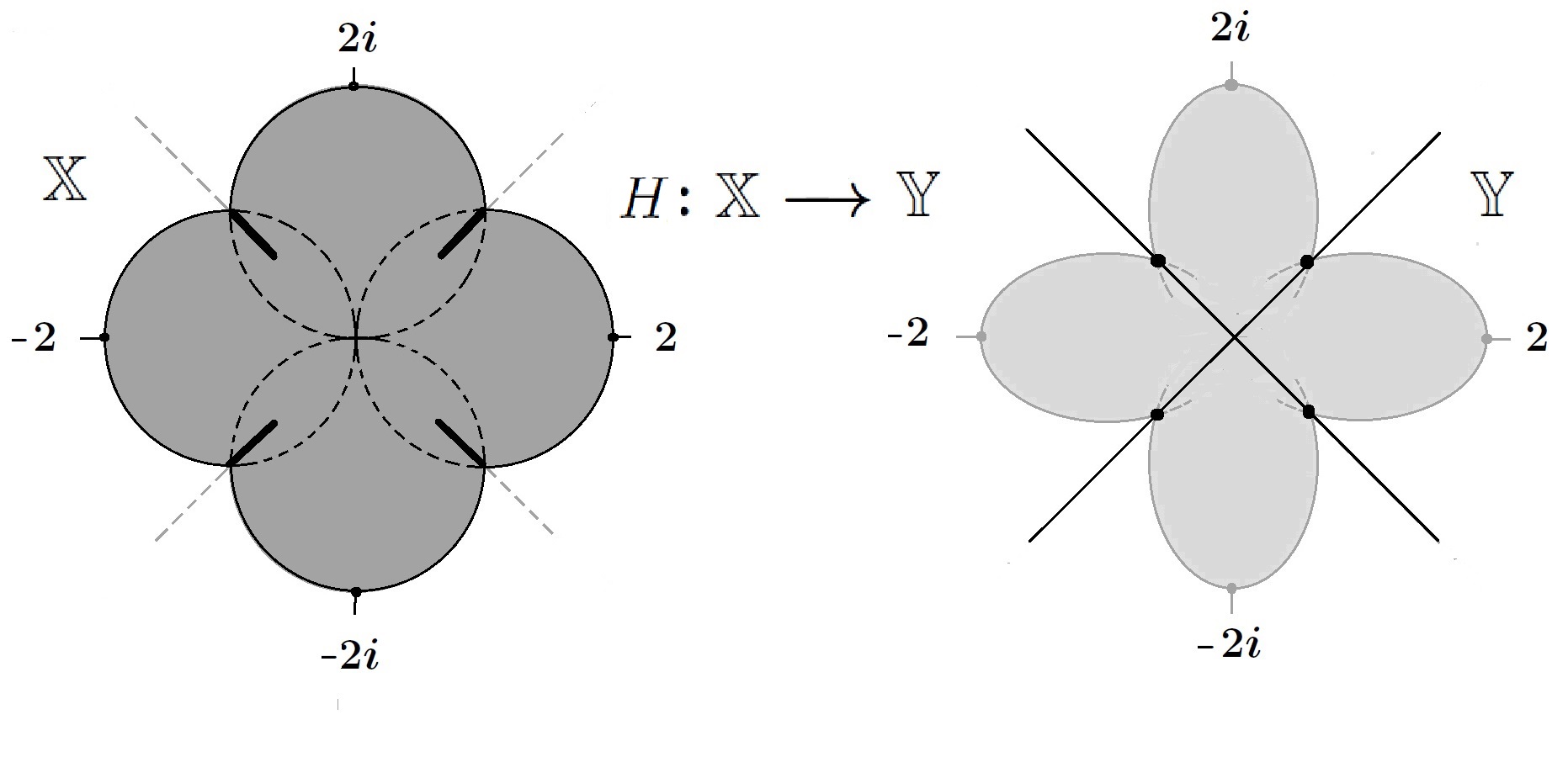
Figure 11. Cuts in a clover are inevitable when $\varepsilon\approx 0\,$. Finding an explicit formula for the length of cuts in terms of $\,\varepsilon\,$, seemingly only a technical problem, is actually quite difficult.

6. An Alternating Process of
Constructing Monotone Hopf-harmonics

In this last section we set out a scheme of possible construction of monotone Hopf-harmonic mapping of a simply connected Jordan domain $\,\mathbb{B}\subset\mathbb{R}^{2}\,$ onto a non-convex Lipschitz domain $\,\mathbb{Y}\subset\mathbb{R}^{2}\,$. The proposed scheme is motivated by the classical Schwarz Alternating Method that was originated in [37, 38, 39] for theoretical studies of conformal mappings and related planar harmonic functions. More recently, this method gained a lot of attention as a very efficient algorithm for parallel computers. There is a substantial literature on Schwarz Alternating Method for general second order elliptic PDEs, beginning in 1951 with S.G. Mikhlin’s paper [32] on convergence of the iterates. See the fundamental work of Lions [28, 29, 30] for far reaching developments and the expository publications by Chan and Mathew [4] and Le Tallec [42], and the book of Smith, Bjorstad and Gropp [40].

We do not attempt to rise and answer the most general questions. Our eventual aim here (not fully realized yet) is to illustrate that the idea of Schwarz remarkable technique can potentially be exercised for monotone solutions of the Hopf-Laplace equation. To emphasize the analogy and differences in our approach, let us take a glimpse of the Schwarz Alternating Method for constructing scalar (real valued) harmonic functions. This scalar case reveals the first major difference; namely, the comparison principle (a powerful tool for scalar harmonic functions) is unavailable when studying complex harmonic homeomorphisms.

The classical Schwarz method works as follows. Let a domain $\,\mathbb{B}\subset\mathbb{R}^{2}\,$ be expressed as union of two overlapping subdomains $\,\mathbb{B}=\mathbb{B}_{1}\cup\mathbb{B}_{2}\,$. We assume that for each of these subdomains one can solve the Dirichlet problem (under any reasonable boundary data). Let a given (reasonable) function $\,g\in\mathscr{C}(\overline{\mathbb{B}})\,$ represent a boundary data for the Dirichlet problem in $\,\mathbb{B}\,$. The alternating process begins with a function $\,g_{1}\,$ on $\,\overline{\mathbb{B}}\,$ that is harmonic on $\,\mathbb{B}_{1}\,$ and has the same values as $\,g\,$ on $\,\partial\mathbb{B}_{1}\,$; call it harmonic replacement of $\,g\in\mathscr{C}(\overline{\mathbb{B}_{1}})\,$. On the remaining part $\,\overline{\mathbb{B}}\setminus\mathbb{B}_{1}\,$, we set $\,g_{1}=g\,$. The next function $\,g_{2}\in\mathscr{C}(\overline{\mathbb{B}})\,$ is harmonic on $\,\mathbb{B}_{2}\,$ with the same values as $\,g_{1}\,$ on $\,\partial\mathbb{B}_{2}\,$, and coincides with $\,g_{1}\,$ on $\,\overline{\mathbb{B}}\setminus\mathbb{B}_{2}\,$. Continuing in this manner, we capture a sequence $\,\{g_{1},g_{2},g_{3},g_{4},...\}\,$ which (under suitable geometric/analytic hypotheses) converges to the solution of the Dirichlet problem in $\,\mathbb{B}\,$, see [32].

The point to make here is that during this process the subdomains $\,\mathbb{B}_{1}\,$ and $\,\mathbb{B}_{2}\,$ stay the same for all time; only the boundary data of the harmonic replacements change. This remains in major contrast with our alternating approach for the monotone Hopf harmonics. Precisely, in our method the subdomains $\,\mathbb{B}_{1}\,$ and $\,\mathbb{B}_{2}\,$ will vary, but their images under the harmonic replacements will always be the same convex domains, say $\,\mathbb{Y}_{1}\,$ and $\,\mathbb{Y}_{2}\,$, respectively. We can make this clear by means of the following example.

6.1. An Example

It involves no loss of generality in assuming that $\,\mathbb{B}\,$ (a simply connected Jordan domain) is the unit disk. In our example, the target $\,\mathbb{Y}\subset\mathbb{R}^{2}\,$ is assembled with two convex subdomains $\,\mathbb{Y}_{1}\,$ and $\,\mathbb{Y}_{2}\,$ such that $\,\mathbb{Y}_{1}\cap\mathbb{Y}_{2}\,\not=\emptyset\,$; these composition of $\,\mathbb{Y}\,$ will stay the same during the entire alternating process. In particular, the target domain $\mathbb{Y}\stackrel{{\scriptstyle\textnormal{def}}}{{=\!\!=}}\mathbb{Y}_{1}\cup\mathbb{Y}_{2}$ is somewhere convex. We shall also assume that $\,\mathbb{Y}\,$ is Lipschitz regular. Furthermore, taking for $\,\mathbb{Y}\,$ a symmetric heart shaped domain, as in Figure 12, considerably eases the arguments.

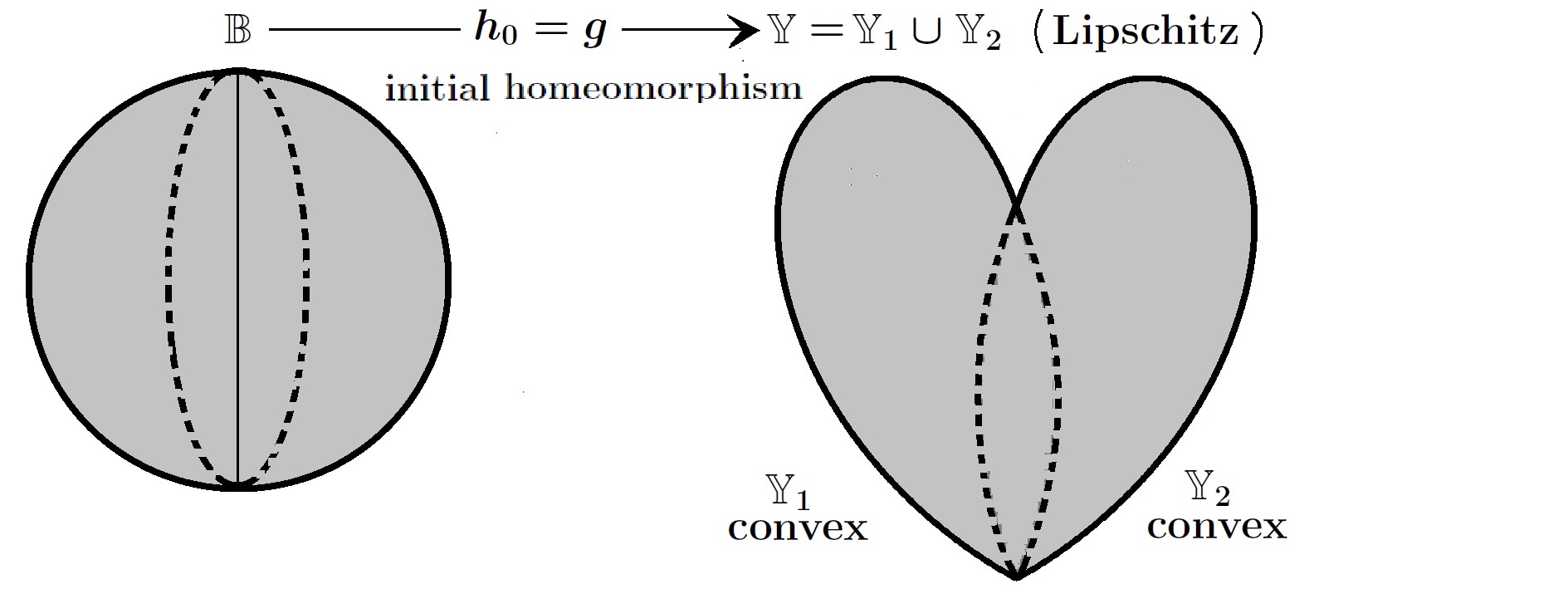
Figure 12. Heart shaped target and the symmetric initial homeomorphism $\,g:\mathbb{B}\xrightarrow[]{{}_{\!\!\textnormal{onto\,\,}\!\!}}\mathbb{Y}\,$.

Let $\,g\colon\overline{\mathbb{B}}\xrightarrow[]{{}_{\!\!\textnormal{onto\,\,}\!\!}}\overline{\mathbb{Y}}$ be a homeomorphism in the Sobolev class $\mathscr{W}^{1,2}(\mathbb{B},\mathbb{C})$. According to Theorem 1.5 there is a unique monotone Hopf-harmonic map $\,h\colon\overline{\mathbb{B}}\xrightarrow[]{{}_{\!\!\textnormal{onto\,\,}\!\!}}\overline{\mathbb{Y}}$ which agrees with $g$ on $\,\partial\mathbb{B}\,$. To simplify matters further, we assume that the boundary data $\,g:\partial\mathbb{B}\xrightarrow[]{{}_{\!\!\textnormal{onto\,\,}\!\!}}\partial\mathbb{Y}\,$ is also symmetric about the vertical axis. Precisely, $\,g(-x,y)=-\overline{g(x,y)}$. By the arguments similar to those for (5.2) and (5.3) It then follows from the uniqueness statement in Theorem 1.5 that $\,h(-x,y)=-\overline{h(x,y)}\,$, everywhere in $\,\overline{\mathbb{B}}\,$. On the other hand, by Theorem 1.5 $\,h^{-1}(\mathbb{Y})\,$ is a simply connected subdomain of $\,\mathbb{B}\,$ in which $\,h\,$ is a harmonic diffeomorphism. Such a subdomain must be the entire disk $\,\mathbb{B}\,$ with a cut (possibly empty) along a segment of the vertical diagonal. Example 4.1 shows that in general such a cut need not be empty. Figure 13 illustrates this case (together with the additional features of the limit map of the alternating process).

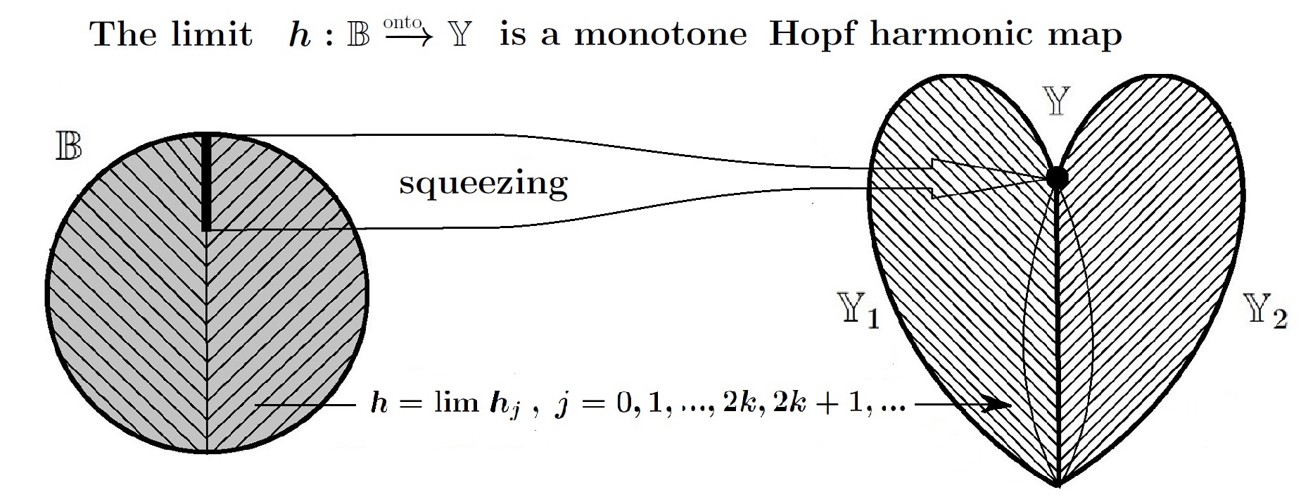
Figure 13. Squeezing phenomenon for a symmetric initial homeomorphism $\,g:\mathbb{B}\xrightarrow[]{{}_{\!\!\textnormal{onto\,\,}\!\!}}\mathbb{Y}\,$.

The idea below is reminiscent of the Schwartz alternating process.

6.2. The iteration process

We shall construct, by induction, a sequence of homeomorphisms $\,h_{j}\in\mathscr{H}_{g}(\overline{\mathbb{B}},\overline{\mathbb{Y}})$. The induction begins with $\,h_{0}\equiv g\,$, see Figure 12, and continues with mappings denoted by $\,h_{1},h_{2},\dots,h_{2k-1},h_{2k},\dots$ for $k=1,2,\dots\,$.

Definition of $h_{1}\colon\overline{\mathbb{B}}\xrightarrow[]{{}_{\!\!\textnormal{onto\,\,}\!\!}}\overline{\mathbb{Y}}$

$$h_{1}=\begin{cases}\textnormal{harmonic replacement of }h_{0}\colon h_{0}^{-1}(\mathbb{Y}_{1})\xrightarrow[]{{}_{\!\!\textnormal{onto\,\,}\!\!}}\mathbb{Y}_{1}\\ h_{0}\;\textnormal{ in }\overline{\mathbb{B}}\setminus h_{0}^{-1}(\mathbb{Y}_{1})\end{cases}$$

Hereafter the term harmonic replacement of a map $\,f\in\mathscr{C}(\overline{\Omega},\mathbb{C})\,$ refers to a map $\,\tilde{f}\in\mathscr{C}(\overline{\Omega},\mathbb{C})\,$ which is harmonic in $\,\Omega\,$ and coincides with $\,f\,$ on $\,\partial\Omega\,$.

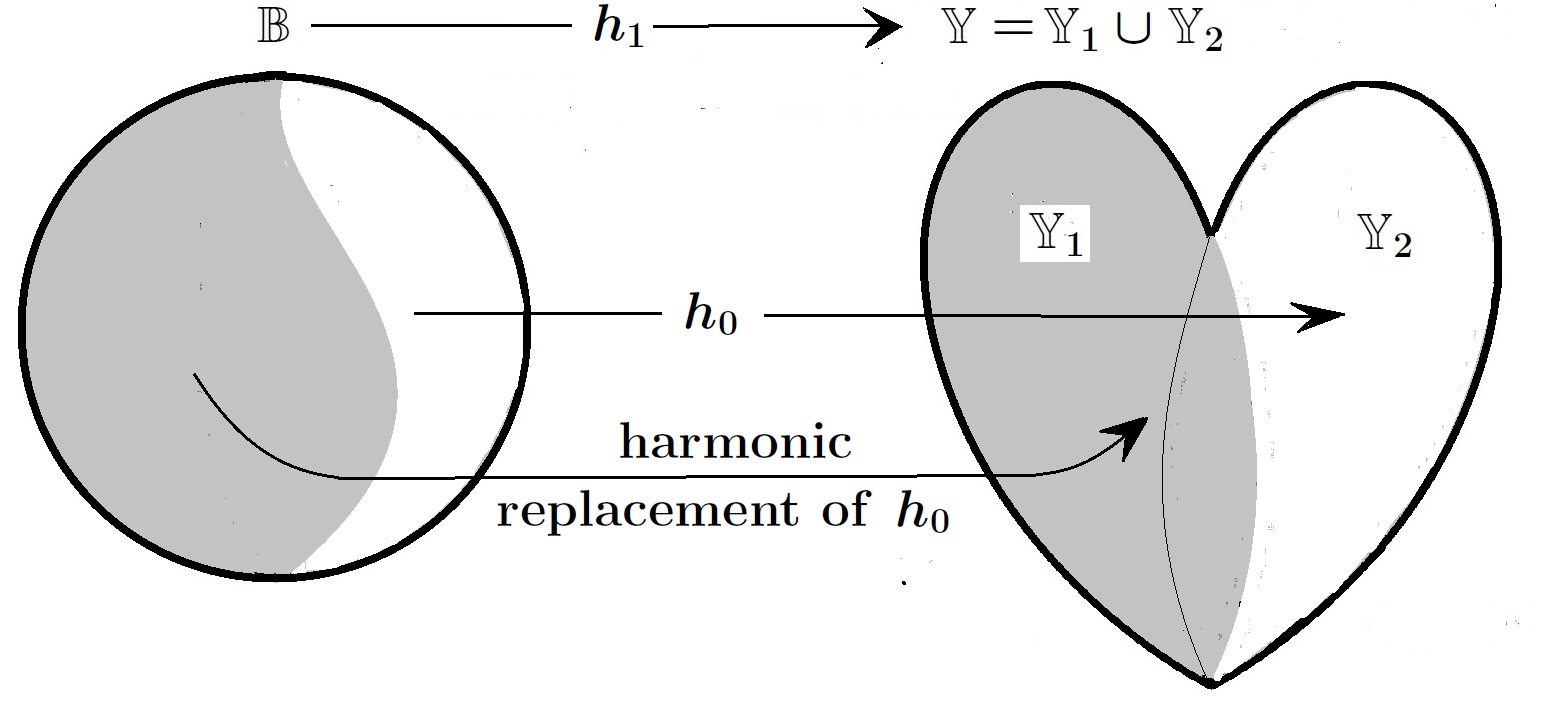
Figure 14. First harmonic replacement; the map $h_{1}\colon h_{0}^{-1}(\mathbb{Y}_{1})\xrightarrow[]{{}_{\!\!\textnormal{onto\,\,}\!\!}}\mathbb{Y}_{1}$

Note that

$$\mathcal{E}[h_{1}]=\int_{\mathbb{B}}\lvert Dh_{1}\rvert^{2}\leqslant\int_{\mathbb{B}}\lvert Dh_{0}\rvert^{2}=\mathcal{E}[h_{0}]\,.$$

Definition of $h_{2}\colon\overline{\mathbb{B}}\xrightarrow[]{{}_{\!\!\textnormal{onto\,\,}\!\!}}\overline{\mathbb{Y}}$

$$h_{2}=\begin{cases}\textnormal{harmonic replacement of }h_{1}\colon h_{1}^{-1}(\mathbb{Y}_{2})\xrightarrow[]{{}_{\!\!\textnormal{onto\,\,}\!\!}}\mathbb{Y}_{2}\\ h_{1}\;\textnormal{ in }\overline{\mathbb{B}}\setminus h_{1}^{-1}(\mathbb{Y}_{2})\end{cases}$$

Thus $\,h_{2}\,$ is harmonic in $\,\mathbb{B}\setminus\partial h_{1}^{-1}(\mathbb{Y}_{2})$.

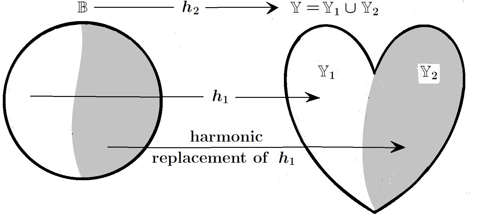
Figure 15. Second harmonic replacement; the map $\,h_{2}\colon h_{1}^{-1}(\mathbb{Y}_{2})\xrightarrow[]{{}_{\!\!\textnormal{onto\,\,}\!\!}}\mathbb{Y}_{2}$

Again, we have

$$\mathcal{E}[h_{2}]\leqslant\mathcal{E}[h_{1}]\leqslant\mathcal{E}[h_{0}]\,.$$

Now, suppose we have defined $h_{2k-1}$ and $h_{2k}$ for some $k\geqslant 1$.
Definition of $h_{2k+1}\colon\overline{\mathbb{B}}\xrightarrow[]{{}_{\!\!\textnormal{onto\,\,}\!\!}}\overline{\mathbb{Y}}$,

$$h_{2k+1}=\begin{cases}\textnormal{harmonic replacement of }h_{2k}\colon h_{2k}^{-1}(\mathbb{Y}_{1})\xrightarrow[]{{}_{\!\!\textnormal{onto\,\,}\!\!}}\mathbb{Y}_{1}\\ h_{2k}\;\textnormal{ in }\overline{\mathbb{B}}\setminus h^{-1}_{2k}(\mathbb{Y}_{1})\end{cases}$$

Definition of $h_{2k+2}\colon\overline{\mathbb{B}}\xrightarrow[]{{}_{\!\!\textnormal{onto\,\,}\!\!}}\overline{\mathbb{Y}}$,

$$h_{2k+2}=\begin{cases}\textnormal{harmonic replacement of }h_{2k+1}\colon h_{2k+1}^{-1}(\mathbb{Y}_{2})\xrightarrow[]{{}_{\!\!\textnormal{onto\,\,}\!\!}}\mathbb{Y}_{2}\\ h_{2k+1}\;\textnormal{ in }\overline{\mathbb{B}}\setminus h^{-1}_{2k+1}(\mathbb{Y}_{2})\end{cases}$$

In each step of our construction we lower the Dirichlet energy, unless the map $\,h_{j}\,$ turns out to be harmonic, in which case the process terminates,

$$\mathcal{E}[h_{0}]\geqslant\dots\geqslant\mathcal{E}[h_{2k+1}]\geqslant\mathcal{E}[h_{2k}]\geqslant\dots\,,\qquad k=0,1,2,\dots$$

Furthermore, $h_{2k+1}$ is a harmonic homeomorphism from $h^{-1}_{2k}(\mathbb{Y}_{1})$ onto $\mathbb{Y}_{1}$ and from $\mathbb{Y}\setminus\overline{h^{-1}_{2k}(\mathbb{Y}_{1})}$ onto $\mathbb{Y}\setminus\overline{\mathbb{Y}_{1}}$. Similarly, $h_{2k+2}$ is a harmonic homeomorphism from $h^{-1}_{2k+1}(\mathbb{Y}_{2})$ onto $\mathbb{Y}_{2}$ and from $\mathbb{Y}\setminus\overline{h^{-1}_{2k+1}(\mathbb{Y}_{2})}$ onto $\mathbb{Y}\setminus\overline{\mathbb{Y}_{2}}$.

6.3. The question of convergence

The family $\{h_{j}\}$ is equicontinuous. This follows from the uniform bound of the modulus of continuity; namely,

$$\lvert h_{j}(x_{1})-h_{j}(x_{2})\rvert^{2}\leqslant\frac{C_{\mathbb{X},\mathbb{Y}}\,\int_{\mathbb{B}}\lvert Dg(x)\rvert^{2}\,\textnormal{d}x}{\log\left(e+1/\lvert x_{1}-x_{2}\rvert\right)}$$

for all $x_{1},x_{2}\in\overline{\mathbb{B}}$, see (3.3). In particular, $\{h_{j}\}$ contains a subsequence converging uniformly on $\overline{\mathbb{B}}$. An obvious question to ask is whether the entire sequence $\{h_{j}\}$ converges; precisely,

Question 6.1.

Does $\{h_{j}\}$ converge uniformly (consequently, weakly in $\mathscr{W}^{1,2}(\mathbb{B},\mathbb{C})$) to a mapping $h\colon\overline{\mathbb{B}}\xrightarrow[]{{}_{\!\!\textnormal{onto\,\,}\!\!}}\overline{\mathbb{Y}}$ (obviously monotone) of smallest Dirichlet energy within the class $\mathscr{M}_{g}(\overline{\mathbb{B}},\overline{\mathbb{Y}})$?

The answer is not known to us in full generality. Whenever the answer to this question is ”yes”, the limit map $\,h\,$ turns out to be the unique monotone Hopf-harmonic solution, as stated in Theorem 1.5.

References

- [1] G. Alessandrini and V. Nesi, Invertible harmonic mappings, beyond Kneser, Ann. Sc. Norm. Super. Pisa Cl. Sci. (5) 8 (2009), no. 3, 451–468.
- [2] J. M. Ball, Convexity conditions and existence theorems in nonlinear elasticity, Arch. Rational Mech. Anal. 63 (1976/77), no. 4, 337–403.
- [3] J. M. Ball, Existence of solutions in finite elasticity, Proceedings of the IUTAM Symposium on Finite Elasticity. Martinus Nijhoff, 1981.
- [4] T. F. Chan and T. P. Mathew, Domain decomposition algorithms, Acta Numerica (1994), 61–143.
- [5] G. Choquet, Sur un type de transformation analytique généralisant la représentation conforme et définie au moyen de fonctions harmoniques, Bull. Sci. Math., 69, (1945), 156–165.
- [6] P. G. Ciarlet, Mathematical elasticity Vol. I. Three-dimensional elasticity, Studies in Mathematics and its Applications, 20. North-Holland Publishing Co., Amsterdam, 1988.
- [7] P. G. Ciarlet and J. Nečas, Injectivity and self-contact in nonlinear elasticity, Arch. Rational Mech. Anal. 97 (1987), no. 3, 171?188.
- [8] J. Cristina, T. Iwaniec, L. V. Kovalev, and J. Onninen, The Hopf-Laplace equation: harmonicity and regularity, Ann. Sc. Norm. Super. Pisa Cl. Sci. (5) 13 (2014), no. 4, 1145–1187.
- [9] J. Douglas, Solution of the problem of Plateau, Trans. Amer. Math. Soc. 33 (1931) 231–321.
- [10] P. Duren, Harmonic mappings in the plane, Cambridge University Press, Cambridge, (2004).
- [11] J. Eells and L. Lemaire, Selected topics in harmonic maps, CBMS Regional Conference Series in Mathematics, 50. American Mathematical Society, Providence, RI, 1983.
- [12] F. Hélein, Harmonic maps, conservation laws and moving frames, 2nd edition. Cambridge University Press, Cambridge, 2002.
- [13] T. Iwaniec, L. V. Kovalev, and J. Onninen Diffeomorphic approximation of Sobolev homeomorphisms, Arch. Ration. Mech. Anal. 201 (2011), no. 3, 1047–1067.
- [14] T. Iwaniec, L. V. Kovalev, and J. Onninen, Hopf differentials and smoothing Sobolev homeomorphisms, Int. Math. Res. Not. IMRN 2012 (2012), no. 14, 3256–3277.
- [15] T. Iwaniec, L. V. Kovalev, and J. Onninen, Lipschitz regularity for inner-variational equations, Duke Math. J. 162 (2013), no. 4, 643–672.
- [16] T. Iwaniec and J. Onninen, Deformations of finite conformal energy: Boundary behavior and limit theorems, Trans. Amer. Math. Soc. 363 (2011), no. 11, 5605–5648.
- [17] T. Iwaniec and J. Onninen, Mappings of least Dirichlet energy and their Hopf differentials, Arch. Ration. Mech. Anal. 209 (2013), no. 2, 401–453.
- [18] T. Iwaniec and J. Onninen, Monotone Sobolev mappings of planar domains and surfaces, Arch. Ration. Mech. Anal. 219 (2016), no. 1, 159–181.
- [19] T. Iwaniec and J. Onninen, Radó-Kneser-Choquet theorem for simply connected domains, Trans. Amer. Math. Soc. to appear.
- [20] T. Iwaniec, G. Verchota and A. Vogel, The Failure of Rank-One Connections, Arch. Rational Mech. Anal. 163 (2002), 125–169.
- [21] Z. Janiszewski, Sur les Coupures du plan, Prace Mat. - Fiz. 26 (1913), p. 55.
- [22] J. Jost, A note on harmonic maps between surfaces, Ann. Inst. H. Poincaré Anal. Non Linéaire 2 (1985), no. 6, 397–405.
- [23] J. Jost, Two-dimensional geometric variational problems, John Wiley & Sons, Ltd., Chichester, 1991.
- [24] H. Kneser, Lösung der Aufgabe 41, Jahresber. Deutsch. Math.-Verein., 35, (1926), 123–124.
- [25] A. Koski and J. Onninen, Sobolev homeomorphic extensions, preprint.
- [26] K. Kuratowski Topology vol II Academic Press, New York-London (1968).
- [27] B. Lévy, S. Petitjean, N. Ray, and J. Maillot, Least squares conformal maps for automatic texture atlas generation, ACM Trans. Graph. 21 (2002), no. 3, 362–371.
- [28] P.-L. Lions, On the Schwarz alternating method. I. First International Symposium on Domain Decomposition Methods for Partial Differential Equations, 1?-42, SIAM, (1988).
- [29] P.-L. Lions, On the Schwarz alternating method. II. Stochastic interpretation and order properties. Domain decomposition methods, 47?-70, SIAM, (1989).
- [30] P.-L. Lions, On the Schwarz alternating method. III. A variant for nonoverlapping subdomains. Third International Symposium on Domain Decomposition Methods for Partial Differential Equations, 202–223, SIAM, (1990).
- [31] A. Marden and K. Strebel, On the ends of trajectories, Differential geometry and complex analysis, 195?204, Springer, Berlin, (1985).
- [32] S.G. Mikhlin, On the Schwarz algorithm, Doklady Akademii Nauk SSSR, n. Ser., (in Russian), 77: 569–-571 (1951).
- [33] C. B. Morrey, The Topology of (Path) Surfaces, Amer. J. Math. 57 (1935), no. 1, 17–50.
- [34] T. Radó, Aufgabe 41., Jahresber. Deutsch. Math.-Verein., 35, (1926), 49.
- [35] R. Raskar, J. van Baar, P. Beardsley, Th. Willwacher, S. Rao, and C. Forlines, iLamps: geometrically aware and self-configuring projectors, ACM Trans. Graph. 22 (2003), no. 3, 809–818.
- [36] R. Schoen and S. T. Yau, On univalent harmonic maps between surfaces, Invent. Math. 44 (1978), no. 3, 265–278.
- [37] H.A. Schwarz, Über einige Abbildungsaufgaben, J. Reine Angew. Math. (1869), 70: 105–-120.
- [38] H.A. Schwarz, Über die Integration der partiellen Differentialgleichung unter vorgeschriebenen Grenz- und Unstetigkeitbedingungen, Monatsberichte der K. Akad. der Wiss. Berlin (1870) 767–795.
- [39] H.A. Schwarz, Über einen Grenzübergang durch alternierendes Verfahren, Vierteljahrsschrift der Naturforschenden Gesellschaft in Zürich, (1870) 272–286.
- [40] B. F. Smith, P. Bjorstad, and W. D. Gropp, Domain decomposition: Parallel multilevel algorithms for elliptic partial differential equations, Cambridge University Press, New York, (1996).
- [41] K. Strebel, Quadratic Differentials, Springer-Verlag, Berlin, 1984.
- [42] P. Le Tallec, Domain decomposition methods in computational mechanics, Computational Mechanics Advances 1 (1994), 121-?220.
- [43] G. T. Whyburn, Non-Alternating Transformations, Amer. J. Math. 56 (1934), no. 1-4, 294–302.
- [44] G. T. Whyburn, Analytic Topology, American Mathematical Society Colloquium Publications, v. 28. American Mathematical Society, New York, (1942).
- [45] J. W. T Youngs, Homeomorphic approximations to monotone mappings, Duke Math. J. 15, (1948) 87–94.