Circular orbits of a ball on a rotating conical turntable

¹ Moscow Institute of Physics and Technology (State University)
141700, Russia, Dolgoprudny, Institutskii per. 9
² Udmurt State University
426034, Russia, Izhevsk, ul. Universitetskaya 1
³Kalashnikov Izhevsk State Technical University
426069, Russia, Izhevsk, ul.Studencheskaya 7

This paper is concerned with the study of the rolling without slipping of a dynamically symmetric (in particular, homogeneous) heavy ball on a cone which rotates uniformly about its symmetry axis. The equations of motion of the system are obtained, partial periodic solutions are found and their stability is analyzed.

1 Introduction

This paper studies the motion of a dynamically symmetric (in particular, homogeneous) heavy ball rolling without slipping on a cone. The cone rotates uniformly about its symmetry axis. To describe the motion, we use the nonholonomic rolling model, assuming that the motion is subject to a linear inhomogeneous nonholonomic constraint, which corresponds to the condition that the velocities of the contacting points on the surface of the ball and the rotating plane be the same. There is no rolling resistance.

This problem is interesting not only from a mechanical point of view (as an example of an integrable system with nonholonomic constraints), but also because there exist various analogies of the system under consideration with systems that are studied in other areas of theoretical physics. For example, the recent papers [5, 4] (see also references therein) make an analogy between the motion of a ball on the surface of a funnel and the motion of a heavy body in a gravitational field. Special attention is given to the rolling of a ball without slipping on a fixed funnel with a variety of shapes (including the case where the surface is conical) to search for Keplerian orbits.

In Ref. [9] an analogy is drawn between the motion of a ball on the surface of a rotating cone and a charged particle in an electromagnetic field, and use is made of approximate equations of motion which ignore the time dependence of the normal to the surface of rolling at the point of contact and the change in the angular velocity of rotation of the ball about the normal.

In this work, we present equations of motion of a ball on a cone taking into account the time dependence of the normal to the surface at the point of contact, and discuss the adequacy of the assumptions made in Ref. [9]

This paper also gives a detailed stability analysis of partial solutions which correspond to rolling along circular trajectories (orbits) at different cone apex angles $\theta\in(0,\pi)$.

2 Derivation of equations of motion

Consider the rolling without slipping of a heavy completely dynamically symmetric (in particular, homogeneous) ball on the surface of a circular cone whose symmetry axis is vertical. The cone rotates about the symmetry axis with constant angular velocity $\boldsymbol{\Omega}$ (Fig. 1).

Let $\theta\in(0,\pi)$ denote the constant apex angle of the cone (measured from the vertical axis). Sometimes, if $\theta\in(0,\pi/2)$, the ball is said to move in a funnel, while if $\theta\in(\pi/2,\pi)$, the ball is said to move on a cone. We will call the surface of rolling a cone for any $\theta$.

We will consider the motion of the ball relative to an inertial (fixed) coordinate system $Oxyz$ in which the axis $Oz$ is directed along the axis of rotation, that is $\boldsymbol{\Omega}=(0,0,\Omega)$.

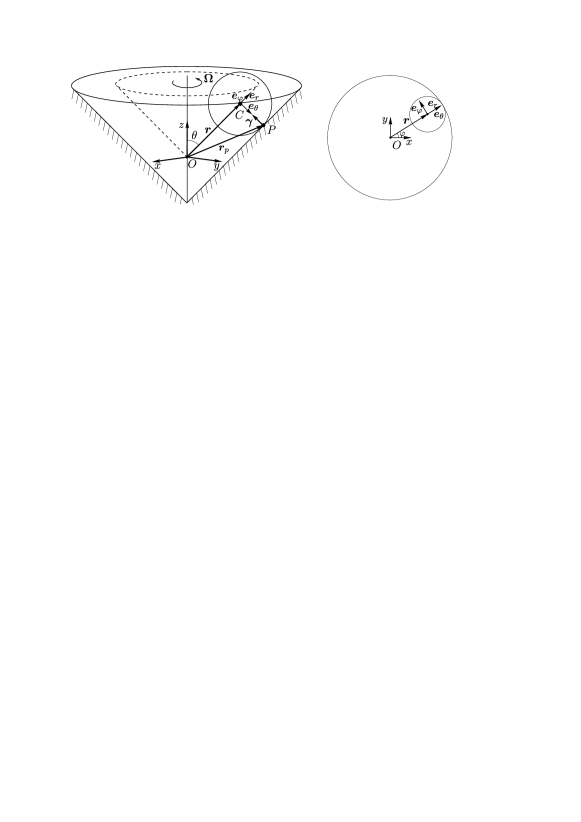
Fig. 1: A ball on a rotating cone. In the left figure, the unit vector $\boldsymbol{e}_{\varphi}$ is directed perpendicularly to the figure plane (from the observer). The right figure shows a view from above, the vector $\boldsymbol{\Omega}$ is directed perpendicularly to the figure plane (to the observer), the unit vectors $\boldsymbol{e}_{\theta},\boldsymbol{e}_{\varphi}$ lie in the same plane perpendicular to the figure plane.

Since there is no slipping, the velocity of the point of contact $P$ on the ball coincides with the velocity of an analogous point on the rotating surface, that is,

$$\boldsymbol{v}+R\boldsymbol{\gamma}\times\boldsymbol{\omega}=\boldsymbol{\Omega}\times\boldsymbol{r}_{p},\quad\boldsymbol{r}_{p}=\boldsymbol{r}-R\boldsymbol{\gamma},$$ (1)

where $\boldsymbol{r}=(x,y,z)$ is the radius vector of the center of mass of the ball, $\boldsymbol{v}=\dot{\boldsymbol{r}}$ and $\boldsymbol{\omega}$ are, respectively, the velocity of the center of mass and the angular velocity of the ball in the coordinate system $Oxyz$, $\boldsymbol{\gamma}$ is the normal at the point of contact, $R$ is the radius of the ball, and $\boldsymbol{r}_{p}$ is the vector directed from the origin of the coordinates to the point of contact $P$. Here and in what follows, all vectors are written in boldface font.

The change in the linear and angular momenta of the ball relative to its center can be written in the form of Newton–Euler equations:

$$m\ddot{\boldsymbol{r}}=\boldsymbol{N}+\boldsymbol{F},\qquad I\dot{\boldsymbol{\omega}}=R\boldsymbol{N}\times\boldsymbol{\gamma},\quad$$ (2)

where $m$ is the mass of the ball, $I$ is the central tensor of inertia of the ball, $\boldsymbol{F}$ is the resultant of the external active forces, and $\boldsymbol{N}$ is the reaction force acting on the ball at the point of contact $P$ (in the general case it can have any direction).

Eliminating the reaction force from the second of Eqs. (2) and performing a vector product by $\boldsymbol{\gamma}$, we obtain

$$\boldsymbol{\gamma}\times\dot{\boldsymbol{\omega}}=\dfrac{mR}{I}\Big{(}\ddot{\boldsymbol{r}}-\boldsymbol{\gamma}(\boldsymbol{\gamma}\cdot\ddot{\boldsymbol{r}})\Big{)}-\dfrac{R}{I}\big{(}\boldsymbol{F}-\boldsymbol{\gamma}(\boldsymbol{\gamma}\cdot\boldsymbol{F})\big{)}.$$ (3)

The vector product on the left-hand side of (3) can be expressed from the derivative of the constraint equation (1) with respect to time:

$$\boldsymbol{\gamma}\times\dot{\boldsymbol{\omega}}=\dfrac{1}{R}\Big{(}-\ddot{\boldsymbol{r}}+\boldsymbol{\Omega}\times\dot{\boldsymbol{r}}+R\dot{\boldsymbol{\gamma}}\times(\boldsymbol{\Omega}-\boldsymbol{\omega})\Big{)}.$$ (4)

Equating the right-hand sides of Eqs.(3) and (4), we obtain an equation governing the evolution of the vector $\boldsymbol{r}$:

$$(k+1)\,\ddot{\boldsymbol{r}}-\boldsymbol{\gamma}\left(\boldsymbol{\gamma}\cdot\ddot{\boldsymbol{r}}\right)=\dfrac{1}{m}\Big{(}\boldsymbol{F}-\boldsymbol{\gamma}\left(\boldsymbol{\gamma}\cdot\boldsymbol{F}\right)\Big{)}+k\,\boldsymbol{\Omega}\times\dot{\boldsymbol{r}}+kR\dot{\boldsymbol{\gamma}}\times(\boldsymbol{\Omega}-\boldsymbol{\omega}),\quad k=\dfrac{I}{mR^{2}},$$ (5)

where $k\geqslant 0$ is the parameter of the system, $k=2/5$ for a homogeneous ball.

We see that, in order to obtain a closed system of equations, we need to define the evolution of the vectors $\boldsymbol{\gamma}$ and $\boldsymbol{\omega}$.

To do so, we first note that the vectors $\boldsymbol{r}$ and $\boldsymbol{\gamma}$ in Eq. (5) are dependent. If the surface on which the center of the ball moves is defined by the equation $\Phi(\boldsymbol{r})=0,$ then the normal vector to this surface is collinear with the normal vector to the surface on which the ball rolls, and is given by the Gauss map

$$\boldsymbol{\gamma}=-\frac{\nabla\Phi(\boldsymbol{r})}{|\nabla\Phi(\boldsymbol{r})|}.$$ (6)

In the case of motion of the ball on the internal surface of the cone, the coordinates of the center of the ball are related by

$$\Phi(\boldsymbol{r})=z^{2}\sin^{2}\theta-(x^{2}+y^{2})\cos^{2}\theta=0.$$ (7)

From this equation we express the normal to the surface using the coordinates of the vector $\boldsymbol{r}$ in explicit form as

$$\gamma_{1}=-\frac{x\cos\theta}{\sqrt{x^{2}+y^{2}}}\,,\quad\gamma_{2}=-\frac{y\cos\theta}{\sqrt{x^{2}+y^{2}}}\,,\quad\gamma_{3}=\sin\theta.$$ (8)

Second, to determine the angular velocity $\boldsymbol{\omega}$, we represent it in the form $\boldsymbol{\omega}=\boldsymbol{\omega}_{\tau}+\omega_{n}\boldsymbol{\gamma},$ where $\omega_{n}=(\boldsymbol{\omega}\cdot\boldsymbol{\gamma})$ is the projection of the angular velocity onto the normal and $\boldsymbol{\omega}_{\tau}$ is the projection of the angular velocity onto the plane tangent to the surface, which is determined from the constraint equation (1):

$$\begin{gathered}\boldsymbol{\omega}_{\tau}=R^{-1}\left(\boldsymbol{\gamma}\times\dot{\boldsymbol{r}}+(\boldsymbol{\Omega}\times(\boldsymbol{r}-R\boldsymbol{\gamma}))\times\boldsymbol{\gamma}\right).\end{gathered}$$ (9)

Thus, to close the system (5), we need to obtain the missing equation for the evolution of the projection of the angular velocity $\omega_{n}$ onto the normal. To find it, we perform a scalar product of the second equation of (2) by $\boldsymbol{\gamma}$, and obtain $k(\dot{\boldsymbol{\omega}},\boldsymbol{\gamma})=0,$ whence using $(\dot{\boldsymbol{\gamma}}\cdot\boldsymbol{\gamma})=0$ we obtain additional equation

$$\dfrac{d\omega_{n}}{dt}=(\boldsymbol{\omega}_{\tau}\cdot\dot{\boldsymbol{\gamma}}).$$ (10)

Thus, Eqs. (5) and (10), with (8) taken into account, form a complete closed system of differential equations governing the motion of a homogeneous ball on the surface of the cone.

In this paper, we shall assume that the ball is acted upon by the gravity force $\boldsymbol{F}=m\boldsymbol{g}$, where $\boldsymbol{g}$ is the free-fall acceleration.

2.1 Equations of motion in spherical coordinates

In this section, as in Ref.[9], we make use of spherical coordinates related to the Cartesian coordinates by

$$x=r\sin\theta\cos\varphi,\quad y=r\sin\theta\sin\varphi,\quad z=r\cos\theta.$$ (11)

In the spherical coordinates, in view of Eq. (11), the surface equation (7) can be reduced to the following very simple form $\theta=\rm{const}.$

Further, we write out the projections of the vectors appearing in Eqs. (1), (5), (10), and their time derivatives onto the spherical basis $\boldsymbol{e}_{r},\boldsymbol{e}_{\theta},\boldsymbol{e}_{\varphi}$ (see Fig. 1), taking into account that $\dot{\theta}=\ddot{\theta}=0$ (for details on the rules of differentiation of vectors in spherical coordinates, see, e.g., Ref.[10]):

$$\begin{gathered}\boldsymbol{r}=r\boldsymbol{e}_{r},\quad\boldsymbol{\gamma}=-\boldsymbol{e}_{\theta},\quad\boldsymbol{\omega}=\omega_{r}\boldsymbol{e}_{r}+\omega_{\theta}\boldsymbol{e}_{\theta}+\omega_{\varphi}\boldsymbol{e}_{\varphi},\\ \quad\dot{\boldsymbol{r}}=\dot{r}\boldsymbol{e}_{r}+r\dot{\varphi}\sin\theta\boldsymbol{e}_{\varphi},\quad\dot{\boldsymbol{\gamma}}=-\dot{\varphi}\cos\theta\boldsymbol{e}_{\varphi},\\ \dot{\boldsymbol{\omega}}=(\dot{\omega}_{r}-\dot{\varphi}\omega_{\varphi}\sin\theta)\boldsymbol{e}_{r}+(\dot{\omega}_{\theta}-\dot{\varphi}\omega_{\varphi}\cos\theta)\boldsymbol{e}_{\theta}+(\dot{\omega}_{\varphi}+\dot{\varphi}(\omega_{\theta}\cos\theta+\omega_{r}\sin\theta))\boldsymbol{e}_{\varphi},\\ \ddot{\boldsymbol{r}}=(\ddot{r}-r\dot{\varphi}^{2}\sin^{2}\theta)\boldsymbol{e}_{r}-r\dot{\varphi}^{2}\cos\theta\sin\theta\boldsymbol{e}_{\theta}+(r\ddot{\varphi}+2\dot{r}\dot{\varphi})\sin\theta\boldsymbol{e}_{\varphi},\\ \boldsymbol{F}=-mg\cos\theta\boldsymbol{e}_{r}+mg\sin\theta\boldsymbol{e}_{\theta},\quad\boldsymbol{\Omega}=\Omega\cos\theta\boldsymbol{e}_{r}-\Omega\sin\theta\boldsymbol{e}_{\theta}.\\ \end{gathered}$$ (12)

Using Eq. (12), the nontrivial projections of Eqs. (5) and (10) onto the basis $\boldsymbol{e}_{r},\boldsymbol{e}_{\theta},\boldsymbol{e}_{\varphi}$ can be represented in the form of five differential first-order equations

$$\begin{gathered}\dot{r}={V_{r}},\quad\dot{\omega}_{\theta}=\dfrac{V_{r}V_{\varphi}}{R}\cos\theta,\quad\dot{V}_{\varphi}=\dfrac{V_{r}}{r}\left(\dfrac{\Omega k}{1+k}-2V_{\varphi}\right),\\ \dot{V}_{r}=rV_{\varphi}^{2}\sin^{2}\theta-\dfrac{kV_{\varphi}}{1+k}\left(r\Omega\sin^{2}\theta+R\cos\theta(\Omega\sin\theta+\omega_{\theta})\right)-\dfrac{g\cos\theta}{1+k},\end{gathered}$$ (13)

$$\dot{\varphi}=V_{\varphi},$$ (14)

and two algebraic equations

$$\omega_{r}=\dfrac{r}{R}(\Omega-V_{\varphi})\sin\theta+\Omega\cos\theta,\quad\omega_{\varphi}=\dfrac{V_{r}}{R}.\\$$ (15)

The equation for $\dot{\varphi}$ (14) decouples from the general system, since the variable $\varphi$ does not appear explicitly in the system (13). This is due to the invariance of the initial system under rotations about the vertical axis.

In addition, the variables $\omega_{r},\omega_{\varphi}$ do not appear explicitly in the resulting differential equations either and can be calculated immediately from Eq.(15) after integrating the system (13).

Thus, the system (13) is closed relative to the unknowns $(r,\omega_{\theta},V_{\varphi},V_{r})$ and completely defines the dynamics of the ball on the cone. In order to restore the motion of the center of mass of the ball in space and to construct its trajectory in the fixed coordinate system $Oxyz$, it is necessary to add the equation (14) to the system (13) and to calculate the dependence of the Cartesian coordinates $(x,y,z)$ on time by using their relation to the spherical coordinates (11).

2.2 Comments on the paper by K. Zengel “The electromagnetic analogy of a ball on a rotating conical turntable”

In the paper by K. Zengel [9], the authors considered the case $\theta=\pi/2+\delta,$ where $\delta$ is a small angle. Using (13), we rewrite in this case the equations governing the evolution of $r,\varphi,\omega_{\theta}$ in the form

$$\begin{gathered}0=\ddot{r}-r\dot{\varphi}^{2}\cos^{2}\delta+\dfrac{r\Omega\dot{\varphi}}{1+k^{-1}}\cos^{2}\delta-G\dfrac{\sin\delta}{1+k},\quad G=g+kR\,\dot{\varphi}(\Omega\cos\delta+\omega_{\theta}),\\ 0=\dfrac{d}{dt}\left(mr^{2}\cos^{2}\delta\left[\dot{\varphi}-\dfrac{k\Omega}{2(1+k)}\right]\right)=\dfrac{d}{dt}\{L_{z}\},\\ \dot{\omega}_{\theta}=-\dfrac{\dot{r}\dot{\varphi}}{R}\sin\delta,\end{gathered}$$ (16)

where $L_{z}$ is a conserved quantity of the system.

The authors [9] also make the following assumption: “the point of contact is assumed to be located directly beneath the center of mass of the ball. For small angles, this approximation holds, but for steep angles and balls with large outer radii, Eq. (3) must be modified”. Based on this, they write equations (16), in which the function $G$ is chosen approximately as follows: $G\approx g.$

We see that in general case this approximation is incorrect, since no account is taken of quantities of the same order of smallness in $\delta$ as $g$. At the same time, we note that the term in the function G neglected by the authors [9]

$$kR\dot{\varphi}(\Omega\cos\delta+\omega_{\theta})$$ (17)

is proportional to the radius of the ball. In the experiments presented in [9], the radius is $R=0.019$ m, and hence the neglected sum (17) at the velocities $\Omega,\omega_{\theta}$ used by the authors [9] is much smaller than the value of $g$, and it can be neglected.

As the radius of the ball increases (the other parameters and initial conditions being equal) the trajectory becomes sensitive to the initial value of the angular velocity $\omega_{\theta}$ (see Fig. 2). In this case, the equations governing the evolution of the angular velocity $\omega_{\theta}$ and the equations for the evolution of $r$ and $\varphi$ do not decouple and must be solved jointly.

In particular, this leads to the result that, for a cone, it is impossible to write the corresponding equations of motion in a natural Hamiltonian form, because the phase space dimension is 5. We note that the problem of Hamiltonization of nonholonomic systems is fairly complicated. Discussions on this topic can be found in [11, 8, 7].

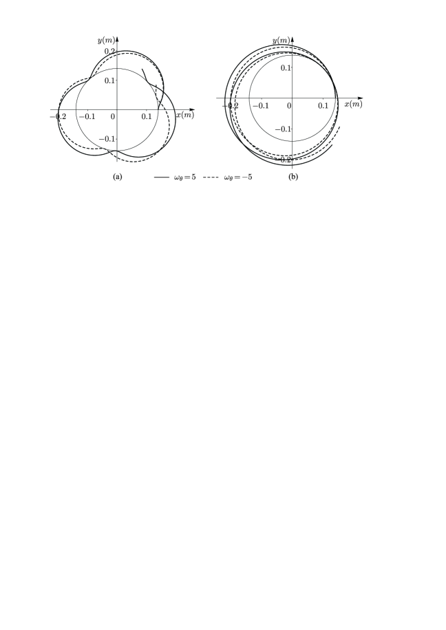
Fig. 2: Projections of the trajectory of the center of mass of the ball onto the horizontal plane for different values of $\omega_{\theta}$ and the parameters $k=2/5,\Omega=7$ rad/s, $g=9.8$ m/s², $R=0.2$ m, $\delta=\pi/180$ for the initial conditions (a) $\dot{\varphi}(0)=0.25$ rad/s and (b) $\dot{\varphi}(0)=1.75$ rad/s (they correspond to values of the quantity $L_{z}/(mr_{0}^{2}\cos^{2}\delta)=\pm 0.75$ rad/s in [9]). All trajectories begin on the right side of the plot at $x=0.14$ m and $y=0$ m. For a comparison, the thin solid line denotes the corresponding periodic trajectories.

3 Periodic solutions

In this section we investigate the circular orbits, i.e., the motion of the center of mass of the ball on a cone in the horizontal plane with some constant frequency.

In the case of the circular periodic motion of the center of mass, the following relations must be satisfied:

$$\begin{gathered}r=r_{0}=\rm{const},\quad V_{r}=0,\quad V_{\varphi}=\omega_{0}=\rm{const},\quad\dot{V}_{r}=0,\quad\dot{V}_{\varphi}=0,\end{gathered}$$ (18)

and $r_{0}>0$.

From the equation for $\dot{\omega}_{\theta}$ (13) we obtain

$$\dot{\omega}_{\theta}=0,\quad\omega_{\theta}=\Omega_{\theta}=\rm{const}.$$ (19)

Consequently, in the case of motion in circular orbits according to Eqs. (18), (19) and the first of Eqs. (13), the derivatives $\dot{r},\dot{\omega}_{\theta},\dot{V}_{r},\dot{V}_{\varphi}$ vanish, which corresponds to definition of the fixed points of the reduced system (13) or periodic motions of the complete system (13)–(14).

The constants $r_{0},\omega_{0},\Omega_{\theta}$ parameterize the circular orbits under consideration. Substituting Eqs. (18) and (19) into the third of Eqs. (13), we obtain an equation that relates these parameters:

$$\omega_{0}^{2}-\dfrac{k\left(r_{0}\Omega\sin^{2}\theta+R\cos\theta(\Omega\sin\theta+\Omega_{\theta})\right)}{r_{0}(1+k)\sin^{2}\theta}\omega_{0}-\dfrac{g\cos\theta}{r_{0}(1+k)\sin^{2}\theta}=0.$$ (20)

Thus, only two parameters are independent. Following [9], as independent parameters we choose $r_{0}$ and $\Omega_{\theta}$, and find the third parameter, $\omega_{0}$, from equation (20) (quadratic in $\omega_{0}$).

Eq. (20) can have two, one or no root $\omega_{0}$, depending on the sign of the discriminant, which has the form

$$\begin{gathered}D(r_{0},\Omega_{\theta})=\dfrac{k^{2}\left(r_{0}\Omega\sin^{2}\theta+R\cos\theta(\Omega\sin\theta+\Omega_{\theta})\right)^{2}}{r_{0}^{2}(1+k)^{2}\sin^{4}\theta}+\dfrac{4g\cos\theta}{r_{0}(1+k)\sin^{2}\theta}.\end{gathered}$$ (21)

Let us analyze in more detail the solution (20) in all possible cases for different $\theta$.

1. When $\theta\in(0,\pi/2)$, the discriminant (21) is positive for all possible values of the system parameters. Consequently, for any values of $r_{0}>0$, $\Omega_{\theta}$ and $\theta\in(0,\pi/2)$ there exist two families of periodic solutions to the system (13)-(14) which correspond to different frequencies of stationary motion

$$\begin{gathered}\omega_{01}(r_{0},\Omega_{\theta})=\dfrac{B(r_{0},\Omega_{\theta})}{2}+\dfrac{\sqrt{D(r_{0},\Omega_{\theta})}}{2},\quad\omega_{02}(r_{0},\Omega_{\theta})=\dfrac{B(r_{0},\Omega_{\theta})}{2}-\dfrac{\sqrt{D(r_{0},\Omega_{\theta})}}{2},\end{gathered}$$ (22)

where $B(r_{0},\Omega_{\theta})$ has been introduced to abbreviate the formula:

$$B(r_{0},\Omega_{\theta})=\dfrac{k\left(r_{0}\Omega\sin^{2}\theta+R\cos\theta(\Omega\sin\theta+\Omega_{\theta})\right)}{(1+k)r_{0}\sin^{2}\theta}.$$ (23)

According to (22), the resulting frequencies correspond to motion of the center of mass of the ball in a circle in opposite directions.

2. When $\theta=\pi/2$ (horizontal plane), equation (20) is transformed to an equation linear in $\omega_{0}$, from which we obtain a well-known expression for the frequency of the circular motion of the ball on the rotating plane in the case of nonholonomic rolling (see [9, 1] and references therein):

$$\omega_{0}=\dfrac{k\Omega}{k+1}.$$

3. When $\theta\in(\pi/2,\pi)$ (which is the case considered in detail in [9]), given $(r_{0},\Omega_{\theta})$, the discriminant (21) can take both positive and negative values. Let us represent it as

$$\begin{gathered}D(r_{0},\Omega_{\theta})=\dfrac{\Omega^{2}k^{2}}{r_{0}^{2}(1+k)^{2}}(r_{0}^{2}+a_{1}r_{0}+a_{2}),\quad\theta=\pi/2+\delta,\quad\delta\in(0,\pi/2),\\ a_{1}=-\dfrac{2\sin\delta}{k^{2}\Omega^{2}\cos^{2}\delta}(Rk^{2}\Omega(\Omega\cos\delta+\Omega_{\theta})+2g(1+k)),\quad a_{2}=\dfrac{R^{2}\sin^{2}\delta}{\Omega^{2}\cos^{4}\delta}(\Omega\cos\delta+\Omega_{\theta})^{2}.\end{gathered}$$ (24)

According to (24), the sign of $D(r_{0},\Omega_{\theta})$ is defined by the polynomial $r_{0}^{2}+a_{1}r_{0}+a_{2}$ quadratic in $r_{0}$. As is well known, on the interval $r_{0}>0$ this polynomial either has no roots and is positive for all $r_{0}$ or has two roots

$$r_{-}(\Omega_{\theta})=-\dfrac{a_{1}}{2}-\dfrac{\sqrt{a_{1}^{2}-4a_{2}}}{2},\quad r_{+}(\Omega_{\theta})=-\dfrac{a_{1}}{2}+\dfrac{\sqrt{a_{1}^{2}-4a_{2}}}{2},$$ (25)

and on the interval $r_{0}\in(r_{-}(\Omega_{\theta}),r_{+}(\Omega_{\theta}))$ this polynomial is negative.

The roots $r_{-}(\Omega_{\theta})$ and $r_{+}(\Omega_{\theta})$ exist if the inequalities $a_{1}^{2}-4a_{2}>0$ and $a_{1}<0$ are satisfied simultaneously. Substituting $a_{1},a_{2}$ from (24) into these inequalities gives

$$\Omega(\Omega\cos\delta+\Omega_{\theta})>-\dfrac{g(k+1)}{Rk^{2}},$$ (26)

$$\Omega(\Omega\cos\delta+\Omega_{\theta})>-2\dfrac{g(k+1)}{Rk^{2}}.$$ (27)

We see that inequality (27) follows from inequality (26) and can be omitted.

Thus, we conclude that if at $\delta\in(0,\pi/2)$ the projection of the angular velocity of the ball onto the normal $\Omega_{\theta}$ satisfies inequality (26), then there exist no periodic solutions to the system (13)-(14) on the interval $r_{0}\in(r_{-}(\Omega_{\theta}),r_{+}(\Omega_{\theta}))$.

Otherwise periodic solutions exist for all $r_{0}\in(0,+\infty)$. Moreover, as in the case $\theta\in(0,\pi/2)$, there exist two different frequencies of periodic motion (22).

Remark 1.

We see that at small $\delta$ the coefficients of the polynomial in (24) are ${a_{1}\sim\delta}$, ${a_{2}\sim\delta^{2}}$. It turns out that $r_{-}(\Omega_{\theta})\sim\delta$ and hence the interval $(0,r_{-}(\Omega_{\theta}))$ is small and is almost unobservable at physical values of the system parameters. That is, the conclusion [9] that there is a minimal value $r_{min}$ for $r_{0}$ on the cone at $\theta\in(\pi/2,\pi)$ is justified from a physical point of view. On the other hand, in our case, $r_{min}=r_{+}(\Omega_{\theta})$, and this expression also differs from $r_{min}$ found in [9]. This difference is also a consequence of the incorrectness (discussed above) of the approximation [9].

4 Stability analysis of periodic solutions

Let us analyze the stability of the periodic solutions of the system (13)–(14), which correspond to fixed points of the reduced system (13). For this, we linearize the system (13) near the partial solution of (18)–(19).

The linearized system can be represented as $\dot{\tilde{{\boldsymbol{z}}}}={\bf L}\tilde{\boldsymbol{z}},$ where ${\bf L}$ is the linearization matrix, $\tilde{\boldsymbol{z}}=\boldsymbol{z}-\boldsymbol{z}_{0}$, $\boldsymbol{z}=(r,\omega_{\theta},V_{r},V_{\varphi})$ is the vector of the variables, and $\boldsymbol{z}_{0}=(r_{0},\Omega_{\theta},0,\omega_{0})$ is the value of the vectors of the variables which corresponds to the partial solution of (18)–(19).

The characteristic equation $\det({\bf L}-\lambda{\bf E})=0$ (with $\lambda$ being its roots) is

$$\lambda^{2}\left(\lambda^{2}+\dfrac{(k+\sin^{2}\theta)\omega_{0}^{2}}{1+k}+\dfrac{2g\cos\theta(\omega_{0}-\omega_{0}^{*})}{r_{0}\omega_{0}(1+k)}\right)=0,\quad\omega_{0}^{*}=\dfrac{k\Omega}{2(1+k)}.$$ (28)

In this case, to facilitate calculations, we have chosen $r_{0}$ and $\omega_{0}$ as independent parameters, and $\Omega_{\theta}$ is uniquely expressed from (20).

Two zero roots of the characteristic equation correspond to the parameters $r_{0},\omega_{0}$ of the family of periodic solution of the system (13)-(14). The nonzero roots of Eq.(28) can be imaginary or real (of different signs) depending on the parameters $r_{0}$ and $\omega_{0}$ and the value of the angular velocity of rotation of the cone $\Omega$.

Let is consider all possible cases for different $\theta$ and $\Omega\geqslant 0$.

1. When $\theta\in(0,\pi/2)$ and $\Omega>0$, the nonzero roots of Eq. (28) are imaginary, the periodic solutions of the system (13)-(14) are linearly stable and of center type in the cases

   1. $\omega_{0}>\omega_{0}^{*}$ or $\omega_{0}<0$ for any $r_{0}$,

   2. $0<\omega_{0}<\omega_{0}^{*}$ and $r_{0}>\dfrac{2g\cos\theta(\omega_{0}^{*}-\omega_{0})}{\omega_{0}^{3}(k+\sin^{2}\theta)}$.

2. When $\theta\in(\pi/2,\pi)$ and $\Omega>0$, the nonzero roots of Eq.(28) are imaginary, the periodic solutions of the system (13)-(14) are linearly stable and of center type in the cases

   1. $0<\omega_{0}<\omega_{0}^{*}$ for any $r_{0}$,

   2. $\omega_{0}>\omega_{0}^{*}$ or $\omega_{0}<0$ and $r_{0}>\dfrac{2g\sin\delta(\omega_{0}-\omega_{0}^{*})}{\omega_{0}^{3}(k+\cos^{2}\delta)},$ where $\delta=\theta-\pi/2$.

3. When $\Omega=0$ and any $\theta\in(0,\pi)$, the nonzero roots of Eq.(28) are imaginary, the family of periodic solutions of the system (13)–(14) is linearly stable and of center type for any $\omega_{0}\not=0$ and $r_{0}.$ When $\omega_{0}=0$, according to Eq. (20), there exist no periodic solutions of the system (13)–(14). For the stability and values of the frequencies of periodic motions at $\Omega=0$, including the case where $k=0$, see also [5].

In other cases, the family of periodic solutions of the system (13)–(14) is linearly unstable and of saddle type. For the sake of illustration, stability and instability regions for $\theta\in(0,\pi/2)$ and $\theta\in(\pi/2,\pi)$ are shown in grey in Fig. 3 on the plane $(\omega_{0},r_{0})$.

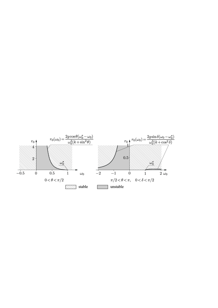
Fig. 3: Stability and instability regions of the periodic solution of the system (13)–(14) on the plane $(r_{0},\omega_{0})$ are constructed for the parameters $k=2/5$, $\Omega=7$ rad/s, $g=9.8$ m/s² and (a) $\theta=89\pi/180$, (b) $\theta=91\pi/180$,

We note that that the characteristic polynomial (28) is invariant under the substitution $(\Omega,\omega_{0},r_{0})\rightarrow(-\Omega,-\omega_{0},r_{0})$. Thus, for $\Omega<0$ analogous regions of stability (instability) of periodic solutions of the system (13), (14) are obtained by a symmetric mapping of regions of stability (instability) in Fig. 3 relative to the vertical axis $\omega_{0}=0$.

5 Conclusion

The analysis of motion of the homogeneous ball on the cone is not restricted to investigating a partial periodic solution. The problem that remains open is that of exploring the rolling of the ball on the cone depending on initial conditions in the general case.

Another open problem is to examine the rolling of the ball with rolling resistance. In the recent paper [1], in the case of motion of a homogeneous ball on a plane, a good agreement was shown between the experimental trajectory and the theoretical trajectory obtained by adding the moment of rolling friction which is proportional to the angular velocity of the ball. Using this friction model, it was shown that all trajectories asymptotically tend to an untwisting spiral.

The preliminary numerical experiment has shown that in the case of motion on a cone with $\theta\in(0,\pi/2)$, as opposed to motion on a plane, ball can either move in an untwisting trajectory (the value of $\rho$ and the height increase in this case) or approach the vertex of the cone (the value of $\rho$ and the height decrease).

References

- [1] A. V. Borisov, T. B. Ivanova, Y. L. Karavaev, and I. S. Mamaev, “Theoretical and experimental investigations of the rolling of a ball on a rotating plane (turntable),” Eur. J. Phys. 39 (6), 065001, 13 (2018).
- [2] A. V. Borisov, I. S. Mamaev, and A. A. Kilin, “The rolling motion of a ball on a surface: New integrals and hierarchy of dynamics” Regul. Chaotic Dyn. 7(2), 201–219 (2002).
- [3] A. V. Borisov, I. S. Mamaev, and I. A. Bizyaev, “The Jacobi Integral in Nonholonomic Mechanics,” Regul. Chaotic Dyn. 20(3), 383–400 (2015).
- [4] L. Q. English , A. Mareno, “Trajectories of rolling marbles on various funnels,” Am. J. Phys. 80(11), 996–1000 (2012).
- [5] Gary D. White, “On trajectories of rolling marbles in cones and other funnels,” Am. J. Phys. 81(12), 890–898 (2013).
- [6] K. Weltner, “Movement of spheres on rotating discs: a new method to Measure coefficients of rolling friction by the central drift,” Mech. Res. Commun. 10(4), 223–232 (1983).
- [7] A. V. Bolsinov, A. V. Borisov, I. S. Mamaev, “Geometrisation of Chaplygin’s reducing multiplier theorem,” Nonlinearity, 28(7), 2307 -2318 (2015).
- [8] K. Ehlers, J. Koiller, J. Montgomery, P. Rios, “Nonholonomic systems via moving frames: Cartan equivalence and Chaplygin Hamiltonization,” The breadth of symplectic and Poisson geometry, Progr. Math., 232, eds. J. E. Marsden, T. S. Ratiu, Birkhäuser, Boston, MA, 75- 120 (2005).
- [9] K. Zengel, “The electromagnetic analogy of a ball on a rotating conical turntable,” Am. J. Phys. 85 (12), 901–907 (2017).
- [10] O. M. O’Reilly, Intermediate dynamics for engineers: a unified treatment of Newton-Euler and Lagrangian mechanics, (Cambridge University Press, New York, 2008).
- [11] T. Ohsawa, O.E. Fernandez, A.M. Bloch, D. V Zenkov, “Nonholonomic HamiltonJacobi theory via Chaplygin Hamiltonization,” J. Geometry and Physics. 61, 1263–1291 (2011).