Simulation of Stylized Facts in Agent-Based Computational Economic Market Models

Abstract

We study the qualitative and quantitative appearance of stylized facts in several agent-based computational economic market (ABCEM) models. We perform our simulations with the SABCEMM (Simulator for Agent-Based Computational Economic Market Models) tool recently introduced by the authors (Trimborn et al. 2019). Furthermore, we present novel ABCEM models created by recombining existing models and study them with respect to stylized facts as well. This can be efficiently performed by the SABCEMM tool thanks to its object-oriented software design. The code is available on GitHub (Trimborn et al. 2018), such that all results can be reproduced by the reader.
Keywords: agent-based models, Monte-Carlo simulations, economic market models, stylized facts, SABCEMM, finite size effects, simulator

1 Introduction

Stylized facts are commonly accepted as persistent empirical pattern in financial data. Probably, the first documented stylized fact is the inequality of income discovered by Pareto in 1897 Pareto (1897). Subsequently, there have been made more statistical observations by Fama and Mandelbrot in the 1960s (Mandelbrot 1997; Brada et al. 1966; Eugene 1963), namely, the non-Gaussian and fat tail behavior of the stock return distribution and volatility clustering. The non-Gaussian behavior can be conveniently studied with the help of a quantile-quantile plot or the excess kurtosis (see appendix definition 2). The tail behavior of an empirical distribution is frequently derived by the Hill estimator (see appendix definition 3). Volatility clustering describes the existence of a positive auto-correlation for squared and absolute stock returns and absence of auto-correlation for raw returns (see appendix definition 1). Nowadays, there have been documented more than 30 stylized facts (Chen et al. 2012; Lux 2008). For a comprehensive overview of stylized facts, we refer to (Cont 2001; Ehrentreich 2007; Campbell et al. 1997; Pagan 1996; Lux 2008).
Standard models in financial literature, such as the capital asset pricing model (Sharpe 1964; Lintner 1965), are build on the efficient market hypothesis by Fama (Fama 1965). Unfortunately, several stylized facts cannot be explained by the efficient market hypothesis and their origin remain unknown (Pagan 1996; Cowan and Jonard 2002; Maldarella and Pareschi 2012). In the past decades, agent-based computational economic market (ABCEM) models have become a powerful tool in order to generate artificial financial data which feature stylized facts. The common goal of many ABCEM models is to shed light on the creation of stylized facts.
ABCEM models consider heterogeneous interacting agents which are studied by means of Monte-Carlo simulations. In contrast to classical financial market models, they share many similarities with interacting particle systems from physics (Sornette 2014; Zschischang and Lux 2001; Lux et al. 2008). Many ABCEM models are able to replicate the most prominent stylized facts of financial markets and are consequently able to provide sufficient conditions for the creation of those. Examples indicate that behavioral aspects of financial investors play an important role in the creation of stylized facts (Cross et al. 2005; Lux 2008; Chen et al. 2012). Further prominent agent-based models are (Kirman 1993; Cont and Bouchaud 2000; Lux and Marchesi 1999; Brock and Hommes 1997). The evident drawback of this computational approach is that all results are based on numerical experiments only. Furthermore, this ansatz only constitutes the sufficient conditions for the generation of stylized facts but does not indicate the necessary ones.
Regarding the simulation of agent-based economic market models, there are two major issues present. First, it has been documented that the appearance of stylized facts are due to finite-size effects as discussed in (Egenter et al. 1999; Zschischang and Lux 2001; Challet and Marslii 2002; Kohl 1997; Hellthaler 1996). In order to exclude such numerical artifacts, it is of major importance to simulate ABCEM models with a large number of agents, which is a computationally expansive undertaking. Secondly, it is difficult to carry out an objective comparison between different ABCEM models, since the models are implemented in different languages and simulated on different hardware. Besides, we experienced difficulties while reproducing the results published in literature. This may well be due to the sensitivity of ABCEM models to their parameters and due to sometimes incomplete information in publications regarding details of the implementation, such as initial values of model quantities.
Therefore, we intend to reproduce established results of multiple models on an identical software architecture to permit an objective comparison. In particular, we investigate the Levy-Levy-Solomon (LLS) model (Levy et al. 1994), the Cross model (Cross et al. 2005) and the Franke-Westerhoff model (Franke and Westerhoff 2012) regarding their long time behavior or their finite size effects.
Finally, we create novel ABCEM models and study them with respect to stylized facts. These new models are built out of well known building blocks, such as a specific market mechanisms or agent designs of other ABCEM models. This approach allows the study of the interplay of different modeling aspects on the creation of stylized facts.
For our simulations, we utilize the recently introduced open source SABCEMM simulator (Trimborn et al. 2019) available on GitHub (Trimborn et al. 2018). There are two major reasons for that choice: First, the SABCEMM simulator is efficient in the sense that it is allows for simulating ABCEM models with up to several million agents on a standard notebook. Secondly, the simulator is build on the idea of building blocks such as market mechanisms or agent designs and thus supports the easy recombination of building blocks of different models as easily as plugging together pieces of a puzzle.
The outline of the paper is as follows: In section 2 we give a short introduction to the SABCEMM simulator. Then we present the simulation results of each model with respect to the reproducibility of the most prominent stylized facts, namely fat-tails, absence of auto-correlation and volatility clustering. Furthermore, we create new models out of existing building blocks of known ABCEM models. Finally, we test these new models with respect to stylized facts. We finish this paper with a short conclusions of this work.

2 The SABCEMM Simulator

The recently introduced open source simulator SABCEMM (Trimborn et al. 2019) is designed especially for large-scale simulations of ABCEM models. This simulator implements an object oriented design leveraging a generalized structure of ABCEM models as defined in (Trimborn et al. 2019). The implementations of the individual ABCEM building blocks are well-separated and the ABCEM model is assembled from the building blocks via an XML-based configuration file. Hence, the evaluation of an ABCEM model using a different building block, such as the market mechanism, requires only a change of the configuration file. If the changed building block does not already exist only this single block has to be implemented. In the following, we present the main conceptual ideas behind the simulator.

SABCEMM is well suited for any economic market model which consists of at least one agent and one market mechanism. An agent is an investor who has a supply of or demand for a certain good or asset, which is traded at the market. The market mechanism determines the price from the demand and supply of all market participants. More precisely, we differentiate between the so called price adjustment process and the excess demand calculator. The latter one aggregates the supply and demand of all market participants (agents) to a single quantity, the excess demand. The former one represents the method of how the market price is fixed based on this excess demand. A schematic picture, which illustrates the presented ideas is shown in Figure 1.

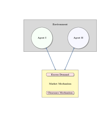
Figure 1: Schematic picture of the abstract ABCEMM model (Trimborn et al. 2019).

The concept of an environment has been first introduced by the authors in (Trimborn et al. 2019). An environment represents possible additional coupling between the agents. Probably, the most famous example for an environment is herding, which is frequently used in ABCEM models. We emphasize that such an environment is not mandatory. For a rigorous mathematical definition of the meta-model which is the foundation of the SABCEMM simulator and a detailed discussion of technical details and computational aspects of SABCEMM, we refer to (Trimborn et al. 2019).

3 Validation and Novel Tests for Known ABCEM Models

In this section we present simulations of the Cross, LLS and Franke-Westerhoff models. We discuss each model separately and demonstrate the advantages of our simulation framework. We study the behavior of the LLS and Cross models for large numbers of agents to investigate if the models exhibit finite-size effects. Furthermore, we study several model variants of the Franke-Westerhoff model with respect to common stylized facts. We emphasize that we provide all necessary information to reproduce the results. To allow for reproducibility, we define the implemented models in detail and present all parameter values and initial states for each model in the appendix A.2. We ran our simulations on an Intel Xeon 64 bit architecture. The input files for all simulations can be found on the GitHub repository of the SABCEMM source code (Trimborn et al. 2018). Additionally, our simulation data is available as a data publication (Trimborn et al. ; Beikirch et al. ).

We provide a short introduction to each model and discuss the appearance of stylized facts for each model separately. For a detailed definition of the implemented models and parameter settings we refer to appendix A.2.

3.1 Cross Model

This section presents results for the Cross model which is inspired by the Ising model (Ising 1925) from physics. In the Cross model, each agent is characterized by his position, long $\sigma_{i}=+1$ or short $\sigma_{i}=-1$ in the market, respectively. Their investment propensity is determined by two tensions: one related to rational agent behavior and the other to irrational agent behavior. They both mimic the role of temperature in the Ising model. The irrational agent behavior takes into account the herding propensity of financial investors. The price process is driven through the change of the excess demand and is additionally perturbed by white noise. The authors Cross et al. show that their model can replicate the most prominent stylized facts of financial markets, namely fat-tails, uncorrelated price returns and volatility clustering. For further modeling details, we refer to (Cross et al. 2005, 2007).

In our simulations, we obtain the same qualitative results as presented in (Cross et al. 2005, 2007). As Figure 2(a) reveals, the price dynamic is influenced heavily by the evolution of the excess demand over time. Furthermore, the absence of auto-correlation in raw price returns can be verified by Figure 4(a). In addition, Figure 3(a) reveals the fat-tail in asset returns. By adding the heteroskedasticity parameter $\theta$, one couples the noise with the excess demand. This leads to volatility clustering as we can see in Figure 4(a). A detailed introduction of the model can be found in appendix A.2.

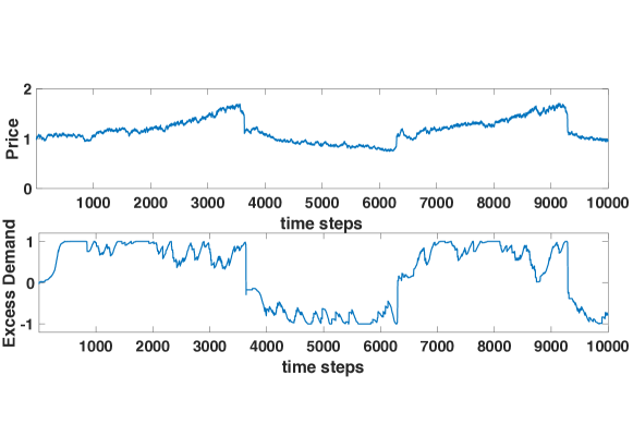
(a) Parameters as in table 3.

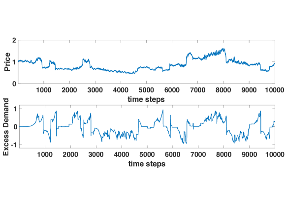
(b) Parameters as in table 3, except $N=5,000,000$ and $\theta=2$.

Figure 2: Development of price and excess demand for the Cross base model.

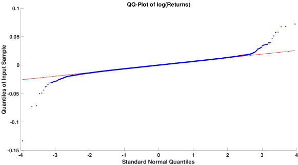
(a) Parameters as in table 3.

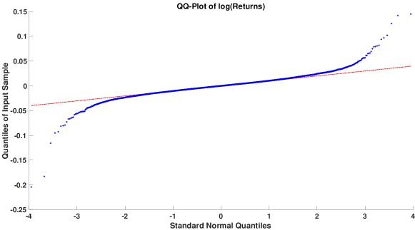
(b) Parameters as in table 3, except $N=5,000,000$ and $\theta=2$.

Figure 3: Fat-tails observed in QQ-plots of the logarithmic returns for the Cross base model.

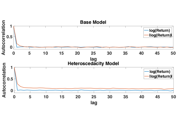
(a) Upper graph: Cross base model with parameters see table 3; lower graph: Cross heteroscedacity model with parameters see table 3 except $\theta=2$.

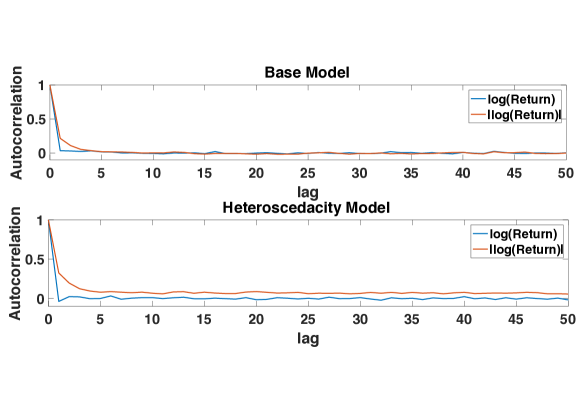
(b) Upper graph: Cross base model with parameters see table 3 and $N=5,000,000$; lower graph: Cross heteroscedacity model with parameters see table 3 except $\theta=2$ and $N=5,000,000$.

Figure 4: Auto-correlation of log-returns and absolute log-returns in the Cross base model and the heteroscedacity models.

Finite Size Effects

In (Cross et al. 2007) the authors claim that their model has no finite size effects. Despite of their claim, all their simulations are performed with 100 agents only. In order to verify their statement, we analyze the model with different numbers of up to five million agents. We ran our simulations with $10,000$ time steps in order to have a sufficiently large sample size. Our simulations support the findings of Cross et al. (see figs. 2(b), 3(b) and 4(b)). Hence, the qualitative behaviour of the Cross model is insensitive to the number of agents, be it $100$ or five million agents.

3.2 LLS Model

In this section, we present results for the LLS model which is one of the earliest and most influential econophysical ABCEM models. In addition, the LLS model is an example of a model assuming a rational market, i.e. the price equilibrates at each time step and the excess demand tends to zero (compare eq. 2). For further details we refer to (Trimborn et al. 2019). Note that the LLS model is subject to critical discussions in literature (Zschischang and Lux 2001). We discuss these crucial findings in detail in this section.

The LLS model considers the wealth evolution of the financial agents. Every agent has to decide in each time step which fraction of wealth he wants to invest in stocks with the remaining wealth being invested in a safe bond. The investment decision is determined by a utility maximization. For modeling details we refer to (Levy et al. 1994, 1995, 1996, 2000).

We define the model and parameter sets in detail in appendix A.2, which is the identical choice as in the earlier studies (Levy et al. 1995, 1996). We consider only one type of financial agent. Figure 5 shows the simulation in the case of noise and no noise added to the investment decision for an agent with fixed memory span of $m=15$. We observe that the noise leads to oscillatory behavior, which coincides with earlier findings in (Levy et al. 1995). Figure 6 shows results for three types of agents with different memory spans $m_{1}=10,\ m_{2}=141,\ m_{3}=256$. The results are qualitatively identical to the results in (Levy et al. 1996).

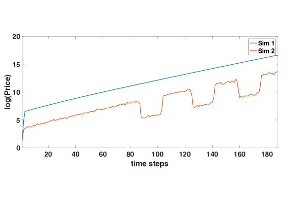
Figure 5: Price evolution of the LLS model with noise $\sigma_{\gamma}=0.2$ (red) and without noise $\sigma_{\gamma}=0$ (blue). Parameters as in table 4

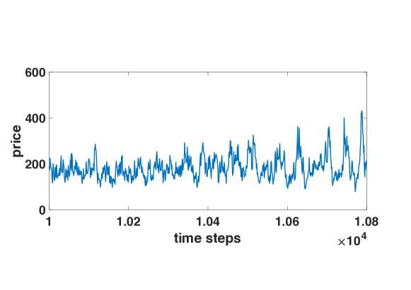
Figure 6: Price evolution of the LLS model with three different investor types. Parameters as in table 5.

Finite Size Effects

It was discovered earlier that the LLS model exhibits finite size effects (Zschischang and Lux 2001). In our simulations, we identify two different kinds of effects caused by a different number of agents. Our simulations are conducted first with 99 agents and then with 999 agents. First, the qq-plot of the logarithmic stock return of both simulations depicted in Figure 7 clearly shows that the number of agents has a tremendous effect on the tail behavior. Secondly, Levy at al. (Levy et al. 1996) claimed that the investor group with the maximum memory becomes the dominant one, meaning they own the maximum amount of wealth. In our simulations, the wealth evolution of different agent groups changes with varying number of agent, as the Figures 8(a) and 8(b) reveal. Thus, we can conclude that the qualitative output of the model changes with respect to the number of agent, which is an undesirable model characteristic.

Figure 7: QQ-Plot of log-returns. Simulations conducted with $99$ agents (left) and $999$ agents (right), respectively. The parameters are set as in table 5.

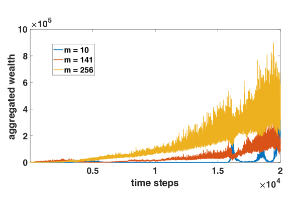
(a) Results for $N=99$ agents.

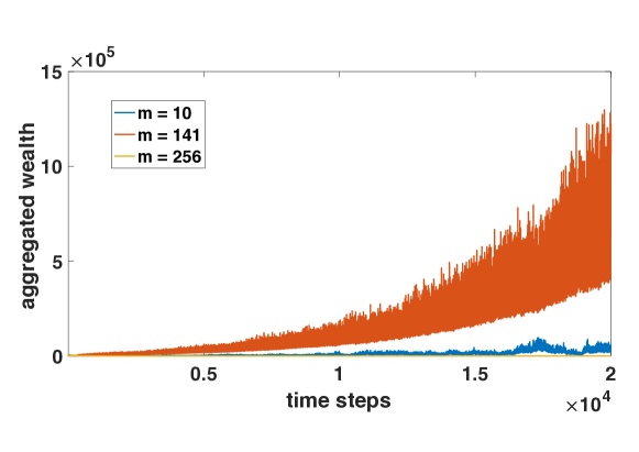
(b) Results for $N=999$ agents.

Figure 8: Aggregate wealth of three equally sized agent groups for different total numbers of agents and parameters as found in table 5.

Discussion of Model Behavior

The simulation in Figure 5 reveals that the deterministic model is characterized by a constant investment proportion. The optimal investment proportion is always located at the boundaries $\gamma\in\{0.01,0.99\}$, determined through the initialization of the return history. This is an absolutely reasonable result, thus the wealth evolution in the original LLS model (Levy et al. 1994) is linear

$$w(t_{k+1})=w(t_{k})+(1-\gamma(t_{k}))\ r+\gamma(t_{k})\ w(t_{k})\ \frac{S(t_{k+1})-S(t_{k})+D(t_{k})}{S(t_{k})},$$ (1)

and the chosen logarithmic utility function is monotonically increasing. In fact, additive noise on the optimal solutions leads to oscillatory behavior. Thus, the investors change between the two possible extreme investments of being fully invested in stocks or bonds. We point out that the noise level is crucial in order to obtain this oscillatory behavior. Figure 9 illustrates the model output for different noise levels.

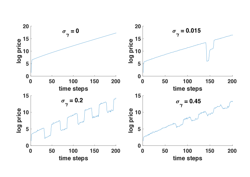
Figure 9: Simulations of the basic LLS model with varying noise levels. Parameters as set in table 4.

Nevertheless Figure 6 seems to indicate chaotic price behavior. The previous simulations (see figs. 7, 8(a) and 8(b)) clearly reveal finite size effects. In our simulations we obtain that also in the noisy case approximately $90\%$ of the investment decisions (pre-noise) are located at the boundaries. Mathematically this is an unsatisfying result since in the expansive optimization process in useless in $90\%$ of the cases. Thus, we may conclude that the LLS model exhibits several undesirable model characteristics.

3.3 Franke-Westerhoff Model

In this section, we consider the Franke-Westerhoff model as discussed in (Franke and Westerhoff 2012). Earlier model variants can be found in (Franke and Westerhoff 2009, 2011). The model studies the evolution of two groups of traders, one group with a chartist strategy and the other with a fundamental strategy. This evolution can be interpreted in the sense of the meta-model introduced in (Trimborn et al. 2019) as the evolution of two representative agents. In each time step, a fraction of the traders adapts their investment strategy by a switching process based on socio-economic factors. These factors are for example a comparison of the agents’ estimated wealth or a herding mechanism. The logarithmic stock price is then driven by the aggregate excess demand of both groups. As a distinct feature of the Franke-Westerhoff model, they employ the concept of structural stochastic volatility as introduced in (Franke and Westerhoff 2009). This means that the demand of chartist and fundamentalist has a stochastic component which takes into account heterogeneity within agent groups and uncertain events. Furthermore, the variance of these random terms differ between both investor groups.

The second distinct feature of the Franke-Westerhoff model is the possibility to choose between two well known switching mechanism. The discrete choice approch (DCA) introduced by Brock and Hommes (Brock and Hommes 1997) or the transition probability approach (TPA) introduced by Weidlich and Haag (Weidlich and Haag 2012) and Lux (Lux 1995).

The authors have shown in several publications (Franke and Westerhoff 2009, 2011, 2012) that their model fits the statistical features of real financial markets such as volatility clustering or fat-tails of stock returns extremely well. Furthermore, they have even employed the method of simulated moments (Franke 2009) in order to fit their model parameters to original financial data.

First, we present the simulations of the Franke-Westerhoff model with discrete choice approach and the behavioral factors herding (H), predisposition (P) and misalignment (M). This model choice can be conveniently abbreviated by DCA-HPM. Figure 10 shows a plot of the auto-correlation function of raw and absolute logarithmic returns. The auto-correlation of raw returns is approximately zero which indicates absence of auto-correlation. In comparison to the raw returns, we obtain a slow algebraic decay in the case of absolute returns. This is known as volatility clustering. In addition, the quantile-quantile plot indicates fat-tails for the logarithmic stock returns.

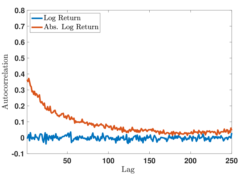
(a) Auto-correlation of logarithmic returns and absolute logarithmic returns.

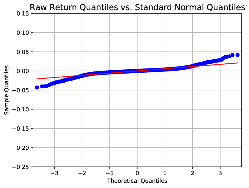
(b) QQ plot of logarithmic returns.

Figure 10: Macroscopic statistics for a DCA-HPM simulation. Parameters as in table 9.

As a second aspect, we investigate the impact of both switching mechanisms. We have simulated the HPM case for the DCA and TPA approach. Figure 11 reveals that the mean fraction of chartists is slightly larger in the DCA approach than in the TPA method (see table 1 as well). Furthermore, Figure 11 shows that the fractions of chartist in the DCA case are much more volatile. We have used the same random number seed in both simulations. Qualitatively, the results of both switching mechanisms do not differ. As presented by Franke and Westerhoff in (Franke and Westerhoff 2011) we run a model contest as well. We have averaged our simulation over 200 runs. Table 1 depicts the different values for the excess kurtosis and the hill estimator of logarithmic returns and the average fractions of chartists. We do not obtain a model which significantly dominates all other choices with respect to reproducing stylized facts. Finally, we have conducted a test in order to study the long time behavior of the model. In fact, Figure 12 depicts that there is no qualitative change in the evolution of prices in the long run.

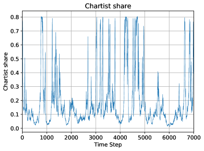
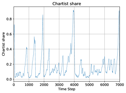
Figure 11: Chartist share for DCA-HPM (left hand side) and TPA-HPM (right hand side) switching mechanisms. Parameters as in table 9 and 12, respectively.

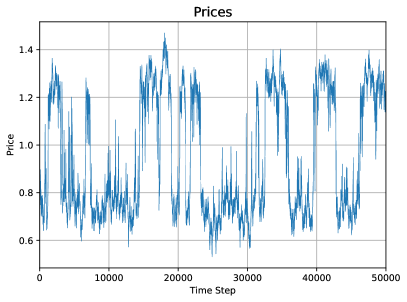
Figure 12: Logarithmic prices for a DCA-HPM simulation (50,000 time steps). Parameters as in table 9, with 50,000 time steps.

	excess kurtosis	Hill estimator	avarage chartist share
TPA-W	5.9512	3.344	0.2813
TPA-WP	7.025	3.1957	0.2507
TPA-HPM	8.614	2.5833	0.1503
DCA-W	8.2023	3.173	0.2577
DCA-WP	7.7600	3.1314	0.2285
DCA-HPM	10.033	2.481	0.1674
DCA-WHP	8.01	3.1192	0.2227
TPA average	7.1967	3.041	0.2274
DCA average	7.99	2.895	0.2179

Table 1: Model contest, parameters as in tables 6 to 12. Each simulation run lasted for 7,000 time steps. The random seed is chosen differently for each repetition, but identical for each of the seven model variants.

4 Novel ABCEM Models

In this section, we demonstrate the flexibility of the SABCEMM simulator by creating new models and adding new features to the Cross model. More precisely, we consider the Cross agents in combination with new market mechanisms. We can show that the precise form of the market mechanism can have a direct impact on the appearance of stylized facts. In addition, we modify the Cross agents by adding a wealth evolution to each agent and study the statistical properties of the wealth evolution.

Wealth Evolution

We consider the original Cross model as defined in appendix A.2. We add a wealth evolution of the type

$$w_{i}(t_{k+1})=w_{i}(t_{k})+\Delta t\ \left[(1-\gamma)\ r+\gamma\frac{S(t_{k})-S(t_{k-1})}{\Delta t\ S(t_{k})}\right]w_{i}(t_{k}),$$

to each Cross agent $i=1,...,N$. The positive constant $r>0$ denotes the interest rate and $\gamma\in(0,1)$ a fixed fraction of stock investments for all agents. The goal is to study the influence of the non-Gaussian return distribution on the wealth distribution. We have plotted the empirical wealth distribution in Figure 14. With increasing $\gamma$, we obtain an increasing excess kurtosis of the wealth distribution. In fact, the excess kurtosis approaches the excess kurtosis of the stock price, which is approximately 6. The results averaged over 100 runs are shown in Figure 13. The qq-plot in Figure 15 clearly shows the asymmetrically fat-tail behavior of the wealth distribution for a fixed $\gamma=1$. Thus, the tails of the wealth distributions are fat for positive values and slim for negative values. This behavior reveals that the tail behavior is translated from the price distribution to the wealth distribution and heavily depends on the investment fraction $\gamma$.

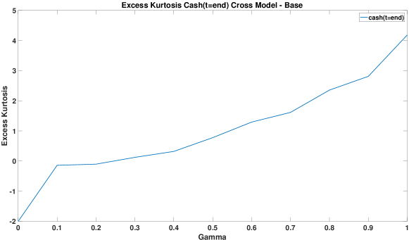
Figure 13: Excess kurtosis for the wealth at the final timestep of the Cross model. Parameters as in table 3 with $w_{i}(t=0)=1$ and $r=0.01$.

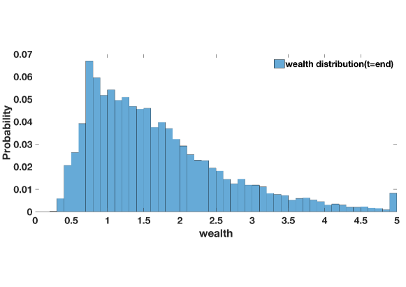
Figure 14: Histogram of the wealth distribution at the final timestep. Parameters as in table 3 with $w_{i}(t=0)=1$ and $r=0.01$.

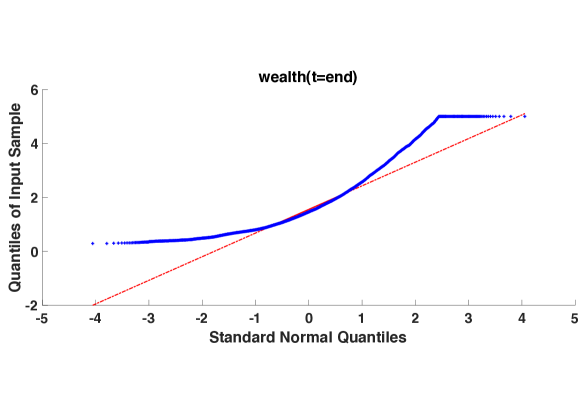
Figure 15: QQ-Plot of the wealth distribution. Parameters as in table 3 with $w_{i}(t=0)=1$ and $r=0.01$.

For future research, we could generalize the microscopic excess demand of the Cross agents by adding a wealth dependency. This would lead to an additional coupling between wealth and stock price behavior.

SDE Discretization

In this section, we again consider the Cross agents, but we change the clearance mechanism. We set the pricing rule to be

$$S(t_{k+1})=S(t_{k})+\Delta t\ F_{Cross}(t_{k},S,ED)+\sqrt{\Delta t}\ S(t_{k})\ (1+\theta\ |ED(t_{k})|)\ \eta,\quad\eta\sim\mathcal{N}(0,1).$$

We choose the Euler-Maruyama discretization of the SDE:

$$dS=F_{Cross}(S,ED)\ dt+S\ (1+\theta\ |ED|)\ dW,$$

where $W$ is a Wiener process and the SDE should be interpreted in the Itô sense. For our first simulation, we set the drift operator $F$ to read:

$$F_{Cross}^{1}(t,S,ED):=S(t)\ \frac{d}{dt}ED(t).$$

As the Figures 16 and 17 reveal, the behavior of this model is identical to the original Cross model. Thus, we have obtained a pricing rule which is a proper time discretization of a time continuous model.

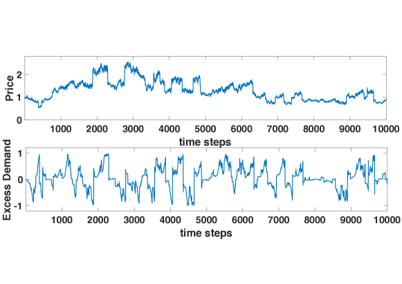
Figure 16: Cross agents with SDE pricing rule. Parameters as in table 3 except $\theta=2$.

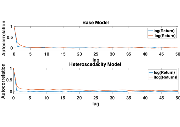
Figure 17: Auto-correlation of log-returns and absolute log-returns in the base model (upper graph, parameters see table 3) and full model (parameters see table 3 except $\theta=2$). We obtain the same behavior as previously in section 3.1.

In a second test we set the drift coefficient to

$$F^{2}_{Cross}(t,S,ED):=S(t)\ ED(t).$$

We study the different impact of the two models on the stock price behavior. Our studies reveal that the the choice $F^{2}_{Cross}$ leads to Gaussian price behavior. We measured this using the excess kurtosis, which we averaged over $100$ runs (see table 2). This is an interesting result, since it reveals the great influence of the drift coefficient on the stock price behavior.

	excess kurtosis
$F^{1}_{Cross},\ \theta=0$	27.0434
$F^{1}_{Cross},\ \theta=2$	22.5530
$F^{2}_{Cross},\ \theta=0$	-0.0044
$F^{2}_{Cross},\ \theta=2$	1.2580

Table 2: Averaged excess kurtosis over 100 runs with different drift functions.

5 Conclusion

We have presented various simulation results using the recently introduced simulator SABCEMM. We have provided a brief introduction to the SABCEMM software. Afterwards, we have carried out several simulations of the LLS model, Cross model and Franke-Westerhoff model. In order to verify that the Cross model is not prone to finite size effects, we ran simulations of up to several million agents. We utilized the well-separated, modular design of SABCEMM, allowing for the recombination of building blocks, to create novel ABCEM models by simply interchanging the market mechanism.

For the previously published ABCEM models, our results and the obtained stylized facts coincide with the findings in literature. The extended numerical studies such as simulations with many agents or long time simulations have supported the validity of these well-known models.
The study of the new ABCEM models based on the agent design of the Cross model has revealed several novel insights. Our studies have shown that the fat-tail property of the stock return influences the tail of the wealth distribution. Interestingly, the fraction of investments in the stock return determines the size of the tail. Hence, the more money is invested in stocks the more prominent is the tail in the wealth distribution. Furthermore, we have seen that the choice of the market mechanism heavily influences the fat-tail property of the stock return data. We conclude that the precise form of the market mechanism is of eminent importance in order to generate realistic stock price data.

These observations lead us to the conclusions that the combination of further building blocks may help to find the origins of stylized facts and to understand the mechanism which create them.

Appendix A Appendix

A.1 Mathematical Appendix

Definition 1.

The auto-correlation for the stationary stochastic process $R(t),\ t>0$ is defined by:

$$C(l):=Corr(R(t+l),R(t))=\frac{Cov(R(t+l),R(t))}{E[(R(t)-\bar{R})^{2}]}=\frac{E[(R(t+l)-\bar{R})\ (R(t)-\bar{R})]}{E[(R(t)-\bar{R})^{2}]},\ l>0$$

The correlation $Corr$ is given by the normalized covariance $Cov$ of two random variables. The auto-correlation function $C(l)\in[-1,1]$ depends on the time shift called lag $l>0$ of the stochastic process.

Definition 2.

The excess kurtosis is defined as the normalized fourth moment of the stationary stochastic stock returns process $R$ minus a correction term, defined by

$$\kappa:=\frac{E[(R-\bar{R})^{2}]}{\sigma^{4}}-3,$$

$$\bar{R}:=E[R],$$

$$\sigma^{2}:=E[(R-\bar{R})^{2}].$$

Definition 3.

The Hill estimator of a sample $X\in\mathbb{R}^{n}_{>0}$ sorted as $x_{1}\geq x_{2}\geq...\ x_{n}$ is defined as

$$H:=\left(\frac{1}{k}\sum_{i=1}^{k}\ln(x_{i})-\ln(x_{k})\right)^{-1},$$

with $k:=\lfloor 0.05*n\rfloor$. For details we refer to (Hill 1975).

A.2 Models

Cross Model

We present the Cross model as defined in (Cross et al. 2005).

We assume a fixed number of $N\in\mathbb{N}$ agents. Each agent decides in each time step, whether he wants to be long or short in the market. Thus, the investment propensity $\sigma_{i},\ 1\leq i\leq N$ of each agent switches between $\sigma_{i}=\pm 1$. The excess demand of all investors at time $[0,\infty)$ is then defined as:

$$ED(t_{k}):=\frac{1}{N}\sum\limits_{i=1}^{N}\sigma_{i}(t_{k}).$$

Furthermore, the model introduces two pressures, the herding pressure and the inaction pressure, which control the switching mechanism.
The inaction pressure is defined by the interval

$$I_{i}=\left[\frac{m_{i}}{1+\alpha_{i}},m_{i}\ (1+\alpha_{i})\right],$$

where $m_{i}$ denotes the stock price of the last switch of agent $i$ and $\alpha_{i}>0$ is the so called inaction threshold. The herding pressure is given by:

$$\begin{cases}c_{i}(t_{k+1})=c_{i}(t_{k})+\Delta t|ED(t_{k})|,&\text{if}\ \sigma_{i}(t_{k})\ ED(t_{k})<0\\ c_{i}(t_{k+1})=c_{i}(t_{k}),&\text{otherwise}.\end{cases}$$

In addition, one defines the herding threshold $\beta_{i}$. The thresholds are chosen once randomly from an i.i.d. random variable, which is uniformly distributed.

$$\alpha_{i}\sim\operatorname{Unif_{c}}(A_{1},A_{2}),\ A_{2}>A_{1}>0,$$

$$\beta_{i}\sim\operatorname{Unif_{c}}(B_{1},B_{2}),\ B_{2}>B_{1}>0.$$

The constants $B_{1}$ and $B_{2}$ have to scale with time, since they correspond to the time units an investor can resist the herding pressure.

$$B_{1}:=b_{1}\cdot\Delta t,$$

$$B_{2}:=b_{2}\cdot\Delta t.$$

Switching mechanism

The switching is then induced if

$$c_{i}>\beta_{i}\ \text{or}\ S(t)\notin I_{i}.$$

After a switch the herding pressure is reset to zero and the inaction interval gets updated as well. The stock price is then driven by the excess demand:

$$S(t_{k+1})=S(t_{k})\ \exp\{(1+\theta\ |ED(t_{k})|)\ \sqrt{\Delta t}\ \eta(t_{k})+\kappa\ \Delta t\ \frac{\Delta ED(t_{k})}{\Delta t}\},$$

$$\sqrt{\Delta t}\ \eta\sim\mathcal{N}(0,\Delta t)$$

$$\Delta ED(t_{k}):=\frac{1}{N}\sum\limits_{i=1}^{N}\sigma_{i}(t_{k})-\frac{1}{N}\sum\limits_{i=1}^{N}\sigma_{i}(t_{k-1}),$$

where $\kappa$ denotes the market depth and $\Delta t>0$ the time step.

Cross model extensions:

One alternative pricing function is given by:

$$S(t_{k+1})=S(t_{k})\ +\Delta t\ \kappa\ \frac{\Delta ED(t_{k})}{\Delta t}\ S(t_{k})+\sqrt{\Delta t}\ F_{Cross}(t_{k},S,ED)\ S(t_{k})\ \eta,$$

Furthermore, we have added the wealth evolution, for a fixed interest rate $r>0$ and fixed investment fraction $\gamma\in(0,1)$:

$$w_{i}(t_{k+1})=w_{i}(t_{k})+\Delta t\ \left[(1-\gamma)\ r+\gamma\frac{S(t_{k})-S(t_{k-1})}{\Delta t\ S(t_{k})}\right]w_{i}(t_{k}).$$

LLS Model

We have implemented the model as defined in (Levy et al. 1994, 1995). We have added one possible time scale to the model. In order to obtain the original model one needs to set $\Delta t=1$.

The model considers $N\in\mathbb{N}$ financial agents who can invest $\gamma_{i}\in[0.01,0.99],\ i=1,...,N$ of their wealth $w_{i}\in\mathbb{R}_{>0}$ in a stocks and have to invest $1-\gamma_{i}$ of their wealth in a safe bond with interest rate $r\in(0,1)$. The investment propensities $\gamma_{i}$ are determined by a utility maximization and the wealth dynamic of each agent at time $t\in[0,\infty)$ is given by

$${w}_{i}(t_{k}) =w_{i}(t_{k-1})$$

$$+\Delta t\left((1-\gamma_{i}(t_{k-1}))\ r\ w_{i}(t_{k-1})+\gamma_{i}(t_{k-1})\ w_{i}(t_{k-1})\ \underbrace{\frac{\frac{{S}(t_{k})-S(t_{k-1})}{\Delta t}+D(t_{k})}{S(t_{k})}}_{=:x(S,t_{k},D)}\right).$$

The dynamics is driven by a multiplicative dividend process. Given by:

$$D(t_{k}):=(1+\Delta t\ \tilde{z})\ D(t_{k-1}),$$

where $\tilde{z}$ is a uniformly distributed random variable with support $[z_{1},z_{2}]$. The price is fixed by the so called market clearance condition, where $n\in\mathbb{N}$ is the fixed number of stocks and $n_{i}(t)$ the number of stocks of each agent.

$$n=\sum\limits_{i=1}^{N}n_{i}(t_{k})=\sum\limits_{k=1}^{N}\frac{\gamma_{k}(t_{k})\ w_{k}(t_{k})}{S(t_{k})}.$$ (2)

The utility maximization is given by

$$\max\limits_{\gamma_{i}\in[0.01,0.99]}E[\log(w(t+\Delta t,\gamma_{i},S^{h}))].$$

with

$$E[\log(w(t_{k-1},\gamma_{i},S^{h}))]=\frac{1}{m_{i}}\sum\limits_{j=1}^{m_{i}}U_{i}\Bigg{(} (1-\gamma_{i}(t_{k}))w_{i}(t_{k},S^{h})\left(1+r\Delta t\right)$$

$$+\gamma_{i}(t_{k})w_{i}(t_{k},S^{h})\Big{(}1+x\big{(}S,t_{k}-j\Delta t,D\big{)}\ \Delta t\Big{)}\Bigg{)}.$$

The constant $m_{i}$ denotes the number of time steps each agent looks back. Thus, the number of time steps $m_{i}$ and the length of the time step $\Delta t$ defines the time period each agent extrapolates the past values. The superscript $h$ indicates, that the stock price is uncertain and needs to be fixed by the market clearance condition. Finally, the computed optimal investment proportion gets blurred by a noise term.

$$\gamma_{i}(t_{k})=\gamma_{i}^{*}(t_{k})+\epsilon_{i},$$

where $\epsilon_{i}$ is distributed like a truncated normally distributed random variable with standard deviation $\sigma_{\gamma}$.

Utility maximization

Thanks to the simple utility function and linear dynamics we can compute the optimal investment proportion in the cases where the maximum is reached at the boundaries. The first order necessary condition is given by:

$$f(\gamma_{i}):=\frac{d}{dt}E[\log(w(t_{k+1},\gamma_{i},S^{h}))]=\frac{1}{m_{i}}\sum\limits_{j=1}^{m_{i}}\frac{\Delta t\ (x\big{(}S,t_{k}-j\Delta t,D\big{)}-r)}{\Delta t\ (x\big{(}S,t_{k}-j\Delta t,D\big{)}-r)\ \gamma_{i}+1+\Delta t\ r}.$$

Thus, for $f(0.01)<0$ we can conclude that $\gamma_{i}=0.01$ holds. In the same manner, we get $\gamma_{i}=0.99$, if $f(0.01)>0$ and $f(0.99)>0$ holds. Hence, solutions in the interior of $[0.01,0.99]$ can be only expected in the case: $f(0.01)>0$ and $f(0.99)<0$. This coincides with the observations in (Samanidou et al. 2007).

Franke-Westerhoff model

The Franke-Westerhoff model (Franke and Westerhoff 2011) considers tow types of agents, chartists and fundamentalists. The demand of each agent reads

$$d^{f}(t_{k})=\phi(P_{f}-P(t_{k}))+\epsilon_{k}^{f},\quad\phi\in\mathbb{R}^{+},\quad\epsilon_{k}^{f}\sim\mathcal{N}(0,\sigma_{f}^{2}),$$ (3)

$$d^{c}(t_{k})=\chi(P(t_{k})-P(t_{k-1}))+\epsilon_{k}^{c},\quad\chi\in\mathbb{R}^{+},\quad\epsilon_{k}^{c}\sim\mathcal{N}(0,\sigma_{c}^{2}),$$ (4)

where $P(t_{k})$ denotes the logarithmic market price and $P_{f}$ denotes the fundamental price. The noise terms $\epsilon_{k}^{f}$ and $\epsilon_{k}^{c}$ are normally distributed, with zero mean and different standard deviations $\sigma_{c}^{2}$ and $\sigma_{f}^{2}$. The second important features are the fractions of the chartist or fundamental population. In that sense the two agents can be seen as representative agents of a population. The fraction of chartists $n^{C}(t_{k})\in[0,1]$ and the fraction of fundamentalitst $n^{F}(t_{k})\in[0,1]$ have to fulfill $n^{C}(t_{k})+n^{F}(t_{k})=1$. Hence, the excess demand can be define as:

$$ED^{F}(t_{k}):=\frac{1}{2}(ed^{f}(t_{k})+ed^{c}(t_{k}))$$ (5)

$$ed^{f}(t_{k}):=2\ n^{f}(t_{k})d^{f}(t_{k})$$

$$ed^{c}(t_{k}):=2\ n^{c}(t_{k}d^{c}(t_{k}).$$ (6)

The pricing equation is then given by the simple rule

$$P(t_{k})=P(t_{k-1})+\mu ED^{F}(t_{k-1}).$$ (7)

Finally, we need to specify the switching mechanism. We have implemented two possible switching mechanisms, the transition probability approach (TPA) (Weidlich and Haag 2012; Lux 1995) and the discrete choice approach (DCA) (Brock and Hommes 1997) approach. In both cases we consider the so called switching index $a(t_{k})\in\mathbb{R}$ which describes the attractiveness of the fundamental strategy over the chartist strategy. Thus, a positive $a(t_{k})$ reflects an advantage of the fundamental strategy in comparison to the chartist and if $a(t_{k})$ is negative we have the opposite situation.

DCA

In the DCA case we obtain

$$n^{f}(t_{k}) =\frac{1}{1+exp(-\beta a(t_{k-1}))},$$

$$n^{c}(t_{k}) =\frac{1}{1+exp(\beta a(t_{k-1}))},$$ (8)

where the parameter $\beta>0$ measures the intensity of choice.

TPA

In the TPA case, we first define switching probabilities

$$\pi^{cf}(a(t_{k-1})) =min[1,\nu\exp(a(t_{k-1}))],$$

$$\pi^{fc}(a(t_{k-1}) =min[1,\nu\exp(-a(t_{k-1}))],$$

where $\pi^{xy}$ is the probability that an agent with strategy x switches to strategy y. The flexibility parameter $\nu$ is a scaling factor for $a(t_{k})$. Then the time evolution of chartist and fundamentalist shares is given by:

$$n^{f}(t_{k}) =n^{f}(t_{k-1})+n^{c}(t_{k-1})\pi^{cf}(a(t_{k-1}))-n^{f}(t_{k-1})\pi^{fc}(a(t_{k-1}))$$

$$n^{c}(t_{k}) =n^{c}(t_{k-1})+n^{f}(t_{k-1})\pi^{fc}(a(t_{k-1}))-n^{c}(t_{k-1})\pi^{cf}(a(t_{k-1}))$$

Finally, we have to specify how the switching index $a(t_{k})$ is calculated. The switching index $a(t_{k})$, encodes how favourable a fundamentalist strategy is over a chartist strategy. The switching index is determined linearly out of the the four principles wealth comparison, predisposition, herding and misalignment.

$$\alpha(t_{k})=\alpha_{w}\ (w^{f}(t_{k})-w^{c}(t_{k}))+\alpha_{0}+\alpha_{h}\ (n^{f}(t_{k})-n^{c}(t_{k}))+\alpha_{m}\ (P(t_{k})-P_{f})^{2},$$

where $\alpha_{w},\alpha_{0},\alpha_{h},\alpha_{m}>0$ are weights respectively scaling factors. The sign $\alpha_{p}\in\mathbb{R}$ determines the predisposition with respect to a fundamental or chartist strategy. The hypothetical wealth $w^{f}(t_{k}),w^{c}(t_{k})$ is determined as follows:

$$w^{f}(t_{k}):=m\ w^{f}(t_{k-1})+(1-m)g^{f}(t_{k}),$$

$$g^{f}(t_{k}):=[exp(P(t_{k}))-exp(P(t_{k-1}))]d^{f}(t_{k-2}),$$

$$w^{c}(t_{k}):=m\ w^{c}(t_{k-1})+(1-m)g^{c}(t_{k}),$$

$$g^{c}(t_{k}):=[exp(P(t_{k}))-exp(P(t_{k-1}))]d^{c}(t_{k-2}).$$

Here, the memory variable $m\in[0,1]$ weights the past performance with the most recent return. For details regarding the modeling we refer to (Franke and Westerhoff 2011).

A.3 Parameter sets

Cross Model

Parameter	Value
$N$	$1000$
$A_{1}$	$0.1$
$A_{2}$	$0.3$
$b_{1}$	$25$
$b_{2}$	$100$
$w_{i}(t=0)$	$1\quad\forall 1\leq i\leq N$
time steps	$10,000$
$\Delta t$	$4\cdot 10^{-5}$
$\kappa$	$0.2$
$\theta$	$0$
$S(t=0)$	$1$

(a) Parameters of Cross model.

Variable	Initial Value
$ED(t=0)$	$\frac{1}{N}\sum\limits_{i=1}^{N}\gamma_{i}(0)$
$c_{i}(t=0)$	$B_{1}+\texttt{rand}\ (B_{2}-B_{1}),\ \forall 1\leq i\leq N$
$m_{i}(t=0)$	$S(t=0),\ \forall 1\leq i\leq N$
$\sigma_{i}(t=0)$	$\operatorname{Unif_{d}}(\{-1,1\})$

(b) Initial values of Cross model.

Table 3: Cross basic setting.

LLS Model

The initialization of the stock return is performed by creating an artificial history of stock returns. The artificial history is modeled as a Gaussian random variable with mean $\mu_{h}$ and standard deviation $\sigma_{h}$. Furthermore, we have to point out that the increments of the dividend is deterministic, if $z_{1}=z_{2}$ holds. We used the C++ standard random number generator for all simulations of the LLS model if not otherwise stated.

Parameter	Value
$N$	$100$
$m_{i}$	$15$
$\sigma_{\gamma}$	$0$ or $0.2$
$r$	$0.04$
$z_{1}=z_{2}$	$0.05$
$\Delta t$	$1$
time steps	200

(a) Parameters of LLS model.

Variable	Initial Value
$\mu_{h}$	$0.0415$
$\sigma_{h}$	$0.003$
$\gamma(t=0)$	$0.4$
$w_{i}(t=0)$	$1000$
$n_{i}(t=0)$	$100$
$S(t=0)$	$4$
$D(t=0)$	$0.2$

(b) Initial values of LLS model.

Table 4: Basic setting of the LLS model.

Parameter	Value
$N$	$99$
$m_{i}$	$10,\ 1\leqslant i\leqslant 33$
	$141,\ 34\leqslant i\leqslant 66$
	$256,\ 67\leqslant i\leqslant 99$
$\sigma_{\gamma}$	$0.2$
$r$	$0.0001$
$z_{1}=z_{2}$	$0.00015$
$\Delta t$	$1$
time steps	$20,000$

(a) Parameters of LLS model.

Variable	Initial Value
$\mu_{h}$	$0.0415$
$\sigma_{h}$	$0.003$
$\gamma_{i}(t=0)$	$0.4$
$w_{i}(t=0)$	$1000$
$n_{i}(t=0)$	$100$
$S(t=0)$	$4$
$D(t=0)$	$0.004$

(b) Initial values of LLS model.

Table 5: Setting for the LLS model (3 agent groups).

Franke-Westerhoff Model

Parameter	Value
$\phi$	$1.0$
$\chi$	$1.2$
$\eta$	$0.991$
$\alpha_{w}$	$1580$
$\alpha_{0}$	$0$
$\alpha_{h}$	$0$
$\alpha_{m}$	$0$
$\sigma_{f}$	$0.681$
$\sigma_{c}$	$1.724$
$\beta$	$1$
$\nu$	$-$
$P_{f}$	$1$
$\mu$	$0.01$
time steps	$7,000$

(a) Parameters for DCA-W.

Variable	Initial Value
$P(t=0)$	1

(b) Initial values DCA-W.

Table 6: DCA-W.

Parameter	Value
$\phi$	$1.0$
$\chi$	$0.9$
$\eta$	$0.987$
$\alpha_{w}$	$2668$
$\alpha_{0}$	$2.1$
$\alpha_{h}$	$0$
$\alpha_{m}$	$0$
$\sigma_{f}$	$0.752$
$\sigma_{c}$	$1.726$
$\beta$	$1$
$\nu$	$-$
$P_{f}$	$1$
$\mu$	$0.01$
time steps	$7,000$

(a) Parameters for DCA-WP.

Variable	Initial Value
$P(t=0)$	1

(b) Initial values DCA-WP.

Table 7: DCA-WP.

Parameter	Value
$\phi$	$1.0$
$\chi$	$0.9$
$\eta$	$0.987$
$\alpha_{w}$	$2668$
$\alpha_{0}$	$2.1$
$\alpha_{h}$	$1.28$
$\alpha_{m}$	$0$
$\sigma_{f}$	$0.741$
$\sigma_{c}$	$2.087$
$\beta$	$1$
$\nu$	$-$
$P_{f}$	$1$
$\mu$	$0.01$
time steps	$7,000$

(a) Parameters for DCA-WHP.

Variable	Initial Value
$P(t=0)$	1

(b) Initial values DCA-WHP.

Table 8: DCA-WHP.

Parameter	Value
$\phi$	$0.12$
$\chi$	$1.5$
$\eta$	$0$
$\alpha_{w}$	$0$
$\alpha_{0}$	$-0.327$
$\alpha_{h}$	$1.79$
$\alpha_{m}$	$18.43$
$\sigma_{f}$	$0.758$
$\sigma_{c}$	$2.087$
$\beta$	$1$
$\nu$	$-$
$P_{f}$	$1$
$\mu$	$0.01$
time steps	$7,000$
random seed	$2661$

(a) Parameters for DCA-HPM.

Variable	Initial Value
$P(t=0)$	1

(b) Initial values DCA-HPM.

Table 9: DCA-HPM.

Parameter	Value
$\phi$	$1.15$
$\chi$	$0.81$
$\eta$	$0.987$
$\alpha_{w}$	$1041$
$\alpha_{0}$	$0$
$\alpha_{h}$	$0$
$\alpha_{m}$	$0$
$\sigma_{f}$	$0.715$
$\sigma_{c}$	$1.528$
$\beta$	$-$
$\nu$	$0.05$
$P_{f}$	$1$
$\mu$	$0.01$
time steps	$7,000$

(a) Parameters for TPA-W.

Variable	Initial Value
$P(t=0)$	1

(b) Initial values TPA-W.

Table 10: TPA-W.

Parameter	Value
$\phi$	$1.0$
$\chi$	$0.83$
$\eta$	$0.987$
$\alpha_{w}$	$2668$
$\alpha_{0}$	$0.376$
$\alpha_{h}$	$0$
$\alpha_{m}$	$0$
$\sigma_{f}$	$0.736$
$\sigma_{c}$	$1.636$
$\beta$	$-$
$\nu$	$0.05$
$P_{f}$	$1$
$\mu$	$0.01$
time steps	$7,000$

(a) Parameters for TPA-WP.

Variable	Initial Value
$P(t=0)$	1

(b) Initial values TPA-WP.

Table 11: TPA-WP.

Parameter	Value
$\phi$	$0.18$
$\chi$	$2.3$
$\eta$	$0.987$
$\alpha_{w}$	$0$
$\alpha_{0}$	$-0.161$
$\alpha_{h}$	$1.3$
$\alpha_{m}$	$12.5$
$\sigma_{f}$	$0.79$
$\sigma_{c}$	$1.9$
$\beta$	$-$
$\nu$	$0.05$
$P_{f}$	$1$
$\mu$	$0.01$
time steps	$7,000$
random seed	$2661$

(a) Parameters for TPA-HPM.

Variable	Initial Value
$P(t=0)$	1

(b) Initial values TPA-HPM.

Table 12: TPA-HPM.

References

- (1) Maximilian Beikirch, Simon Cramer, Martin Frank, Philipp Joachim Otte, Emma Pabich, and Torsten Trimborn. Dataset for simulation of stylized facts in agent-based computational economic market models. URL https://publications.rwth-aachen.de/record/749924.
- Brada et al. (1966) Josef Brada, Harry Ernst, and John Van Tassel. Letter to the editor—the distribution of stock price differences: Gaussian after all? Operations Research, 14(2):334–340, 1966.
- Brock and Hommes (1997) William A Brock and Cars H Hommes. A rational route to randomness. Econometrica: Journal of the Econometric Society, pages 1059–1095, 1997.
- Campbell et al. (1997) John Y Campbell, Andrew Wen-Chuan Lo, Archie Craig MacKinlay, et al. The econometrics of financial markets, volume 2. princeton University press Princeton, NJ, 1997.
- Challet and Marslii (2002) D. Challet and M. Marslii. Criticality and finite size effects in a simple realistic model of stock market. Working Paper Department of Theoretical Physics, Oxford University, INFM, Trieste-SISSA Unit, Trieste, 2002.
- Chen et al. (2012) Shu-Heng Chen, Chia-Ling Chang, and Ye-Rong Du. Agent-based economic models and econometrics. The Knowledge Engineering Review, 27(02):187–219, 2012.
- Cont (2001) Rama Cont. Empirical properties of asset returns: stylized facts and statistical issues. 2001.
- Cont and Bouchaud (2000) Rama Cont and Jean-Philipe Bouchaud. Herd behavior and aggregate fluctuations in financial markets. Macroeconomic dynamics, 4(2):170–196, 2000.
- Cowan and Jonard (2002) Robin Cowan and Nicolas Jonard. Heterogenous agents, interactions and economic performance, volume 521. Springer Science & Business Media, 2002.
- Cross et al. (2005) Rod Cross, Michael Grinfeld, Harbir Lamba, and Tim Seaman. A threshold model of investor psychology. Physica A: Statistical Mechanics and its Applications, 354:463–478, 2005.
- Cross et al. (2007) Rod Cross, Michael Grinfeld, Harbir Lamba, and Tim Seaman. Stylized facts from a threshold-based heterogeneous agent model. The European Physical Journal B, 57(2):213–218, 2007.
- Egenter et al. (1999) E Egenter, T Lux, and D Stauffer. Finite-size effects in monte carlo simulations of two stock market models. Physica A: Statistical Mechanics and its Applications, 268(1):250–256, 1999.
- Ehrentreich (2007) Norman Ehrentreich. Agent-based modeling: The Santa Fe Institute artificial stock market model revisited, volume 602. Springer Science & Business Media, 2007.
- Eugene (1963) Fama Eugene. The distrigbution of the daily differences of the logarithms of stock prices. In Ph.D. Thesis. Graduate School of Business University of Chicago, 1963.
- Fama (1965) Eugene F Fama. The behavior of stock-market prices. The journal of Business, 38(1):34–105, 1965.
- Franke (2009) Reiner Franke. Applying the method of simulated moments to estimate a small agent-based asset pricing model. Journal of Empirical Finance, 16(5):804–815, 2009.
- Franke and Westerhoff (2009) Reiner Franke and Frank Westerhoff. Validation of a structural stochastic volatility model of asset pricing. Christian-Albrechts-Universität zu Kiel. Department of Economics, 2009.
- Franke and Westerhoff (2011) Reiner Franke and Frank Westerhoff. Estimation of a structural stochastic volatility model of asset pricing. Computational Economics, 38(1):53–83, 2011.
- Franke and Westerhoff (2012) Reiner Franke and Frank Westerhoff. Structural stochastic volatility in asset pricing dynamics: Estimation and model contest. Journal of Economic Dynamics and Control, 36(8):1193–1211, 2012.
- Hellthaler (1996) T Hellthaler. The influence of investor number on a microscopic market model. International Journal of Modern Physics C, 6(06):845–852, 1996.
- Hill (1975) Bruce M Hill. A simple general approach to inference about the tail of a distribution. The annals of statistics, pages 1163–1174, 1975.
- Ising (1925) Ernst Ising. Beitrag zur theorie des ferromagnetismus. Zeitschrift für Physik A Hadrons and Nuclei, 31(1):253–258, 1925.
- Kirman (1993) Alan Kirman. Ants, rationality, and recruitment. The Quarterly Journal of Economics, 108(1):137–156, 1993.
- Kohl (1997) R Kohl. The influence of the number of different stocks on the levy–levy–solomon model. International Journal of Modern Physics C, 8(06):1309–1316, 1997.
- Levy et al. (2000) Haim Levy, Moshe Levy, and Sorin Solomon. Microscopic simulation of financial markets: from investor behavior to market phenomena. Academic Press, 2000.
- Levy et al. (1994) Moshe Levy, Haim Levy, and Sorin Solomon. A microscopic model of the stock market: cycles, booms, and crashes. Economics Letters, 45(1):103–111, 1994.
- Levy et al. (1995) Moshe Levy, Haim Levy, and Sorin Solomon. Microscopic simulation of the stock market: the effect of microscopic diversity. Journal de Physique I, 5(8):1087–1107, 1995.
- Levy et al. (1996) Moshe Levy, Nathan Persky, and Sorin Solomon. The complex dynamics of a simple stock market model. International Journal of High Speed Computing, 8(01):93–113, 1996.
- Lintner (1965) John Lintner. Security prices, risk, and maximal gains from diversification. The journal of finance, 20(4):587–615, 1965.
- Lux (1995) Thomas Lux. Herd behaviour, bubbles and crashes. The economic journal, pages 881–896, 1995.
- Lux (2008) Thomas Lux. Stochastic behavioral asset pricing models and the stylized facts. Technical report, Economics working paper/Christian-Albrechts-Universität Kiel, Department of Economics, 2008.
- Lux and Marchesi (1999) Thomas Lux and Michele Marchesi. Scaling and criticality in a stochastic multi-agent model of a financial market. Nature, 397(6719):498–500, 1999.
- Lux et al. (2008) Thomas Lux et al. Applications of statistical physics in finance and economics. Technical report, Kiel working paper, 2008.
- Maldarella and Pareschi (2012) Dario Maldarella and Lorenzo Pareschi. Kinetic models for socio-economic dynamics of speculative markets. Physica A: Statistical Mechanics and its Applications, 391(3):715–730, 2012.
- Mandelbrot (1997) Benoit B Mandelbrot. The variation of certain speculative prices. In Fractals and scaling in finance, pages 371–418. Springer, 1997.
- Pagan (1996) Adrian Pagan. The econometrics of financial markets. Journal of empirical finance, 3(1):15–102, 1996.
- Pareto (1897) Vilfredo Pareto. Cours d’économie politique, professé à l’université de lausanne. tome second, 1897.
- Samanidou et al. (2007) Egle Samanidou, Elmar Zschischang, Dietrich Stauffer, and Thomas Lux. Agent-based models of financial markets. Reports on Progress in Physics, 70(3):409, 2007.
- Sharpe (1964) William F Sharpe. Capital asset prices: A theory of market equilibrium under conditions of risk. The journal of finance, 19(3):425–442, 1964.
- Sornette (2014) Didier Sornette. Physics and financial economics (1776–2014): puzzles, ising and agent-based models. Reports on Progress in Physics, 77(6):062001, 2014.
- Trimborn et al. (2018) T. Trimborn, P. Otte, S. Cramer, M. Beikirch, E. Pabich, and M. Frank. Simulator for agent based computational economic market models (SABCEMM). https://github.com/SABCEMM/SABCEMM, 2018.
- (42) Torsten Trimborn, Philipp Otte, Simon Cramer, Max Beikirch, Emma Pabich, and Martin Frank. Data set of SABCEMM - a simulation framework for agent-based computational economic market models. http://dx.doi.org/10.18154/RWTH-2017-09142.
- Trimborn et al. (2019) Torsten Trimborn, Philipp Otte, Simon Cramer, Maximilian Beikirch, Emma Pabich, and Martin Frank. SABCEMM: A simulator for agent-based computational economic market models. Computational Economics, Jul 2019. ISSN 1572-9974. doi: 10.1007/s10614-019-09910-1. URL https://doi.org/10.1007/s10614-019-09910-1.
- Weidlich and Haag (2012) Wolfgang Weidlich and Günter Haag. Concepts and models of a quantitative sociology: the dynamics of interacting populations, volume 14. Springer Science & Business Media, 2012.
- Zschischang and Lux (2001) Elmar Zschischang and Thomas Lux. Some new results on the levy, levy and solomon microscopic stock market model. Physica A: Statistical Mechanics and its Applications, 291(1):563–573, 2001.