Light hidden photon production in high energy collisions
Abstract
The visible and dark sectors of particle physics can be connected via the kinetic mixing between the ordinary () and hidden photon (). If the latter is light its production in high energy collisions of ordinary particles occurs via the oscillations similarly to the neutrino processes. Generically, the experiments are insensitive to mass of the hidden photon, if it is lighter than 1 MeV, and it does not decay into -pair. Still, one can use the missing energy and scattering off the detector as signatures to search for light hidden photon. Presence of media suppresses production of the light vectors making the experiments insensitive to the entire model. In media the light hidden photon production is typically suppressed due to the dump of the oscillations making the experiments insensitive to the entire model. We present analytic formulas for the light hidden photon production, propagation and detection valid for searches at colliders and beam-target experiments and apply them to estimate the impact on the sensitivities of NA64, FASER, MATHUSLA, SHiP, T2K, DUNE and NA62 for the background-free case.
1 Introduction
New physics can involve GeV-scale and even lighter particles, the pattern argued to be preferable when the gauge hierarchy problem is addressed [1, 2]. These new particles can be directly searched for in high-intensity collision experiments operating at collider or fixed-target facilities. They include universal experiments like those running at the LHC, long-baseline neutrinos oscillation experiments exploiting proton beams incident on target (DUNE, T2K) and specially designed projects with high-intensity beams dedicated to new physics hunting (NA64, SHiP, MATHUSLA). Generically, whenever very light particles are concerned, astrophysical processes exhibit a higher sensitivity than the direct searches, but the latter naturally earn a higher confidence, and we concentrate on them.
The new particles, if light, must be singlet with respect to the gauge group of the Standard Model of particle physics (SM). Otherwise, absence of their traces in numerous experiments performed so far would be difficult to explain. If the new singlet is a Lorenzian vector, , its most natural effective interaction with the SM fields is via so-called vector portal — renormalizable mixing between the gauge-invariant kinetic terms of and photon . Below the electroweak scale around 100 GeV the corresponding lagrangian reads
| (1) |
where is the hidden photon mass emerged presumably due to the Higgs mechanism operating in the hidden sector. The kinetic mixing with the ordinary photon in (1) solely defines the hidden photon phenomenology associated with the SM particles: can be produced by a virtual photon and can decay into the SM particles via a virtual photon wherever kinematically allowed. The hidden photon can also effectively scatter off the electrically charged SM particles because of this mixing. Besides, in the hidden sector can couple to dark matter particles [3] hence forming a gate between the visible and dark Worlds. From phenomenological side, the couplings to particles from the hidden sector imply a possibility of invisible decay mode for , which alters the strategy of its searches [4].
In this paper we study phenomenology of the hidden photon, lighter than 1 MeV, when the decay mode into is forbidden. And we take the limit where the hidden photons participate in processes (e.g. emerge, scatter, etc) being ultra-relativistic in the laboratory frame, . Then in many cases the interaction of the hidden photon with the SM particles happens via oscillations , rather than via the Compton scattering (see e.g. [5]). In particular, applying oscillations to describe the hidden photon behavior in a nuclear reactor it has been recently found [6] that, generically, there are no chances to produce too light hidden photon there. The reason is that the visible photon either gets absorbed or scatters in media before oscillating into the hidden photon. The electromagnetic interactions of the visible photon in media effectively suppress the oscillations with respect to the vacuum case. The only exception is a resonance region, where the hidden photon mass coincides with the plasma frequency in the media, where the photons propagate.
In the main part of the paper we give formulas to describe the visible photon conversion to the hidden photon and back which could be useful for several classes of experiments. Usually the accelerator experiments do not provide bounds on the visible-to-hidden photon mixing for MeV, unless specially designed. However, in many cases they can extend the limits to this region, and our formulas will help to do it. We discuss their applicability and prospects of these experiments to explore the models with the light hidden photon.
The plan of the paper is as follows. We present the detailed description of the oscillations in Sec. 2. In Sec. 3 we apply this approach to calculate the light hidden photon production probability for the cases of collisions in vacuum (e.g. a collider) and in matter (e.g. a beam-dump experiment). Generally, the hidden photon can be detected either via disappearance of the visible photon or via appearance of a visible photon from nowhere (“light shining through the wall”). The both processes for the light ultrarelativistic hidden photon are described as hidden-to-visible photon oscillations and discussed in detail in Sec. 4. Finally, in Sec. 5 we estimate the conversion probability for several presently ongoing and future experiments, and investigate the impact of our findings on their prospects in probing models with light hidden photon assuming zero background and 100% detection efficiency (that implies the most optimistic numbers). We summarize in Sec. 6 emphasizing the necessary conditions for the resonance amplification of the hidden photon production in accelerator experiments.
2 Oscillations between visible and hidden photons
In this Section we present main formulas describing oscillations of the visible–hidden photon system in vacuum and media.
In the interesting case of small mixing, , it is convenient to replace with , so that in the new variables the kinetic term in lagrangian (1) is diagonal, but mixing emerges in the mass term, instead. State remains sterile with respect to the SM gauge interactions and we call it the hidden photon state. The system evolution written in terms of the new fields allows for a very simple description via oscillations. Namely, while the electromagnetic current produces a quantum wave-packet of photon , the states which propagate — eigenvectors of the Hamiltonian — are mixtures of and . As it follows from (1) the Hamiltonian describing the system () in the ultrarelativistic regime in vacuum has the form
| (2) |
up to corrections of order in its diagonal part. Here is the photon energy. Note in passing that we consider here only two transverse polarizations of the massive hidden photon. As for the third, longitudinal polarization, it is out of interest here, because its production in the processes under discussion is suppressed, as compared to the transverse polarization modes, by factor , see Ref. [7] for the details. The corresponding time evolution between the “interaction eigenstates”, i.e. and , is very similar to the oscillations between neutrino flavours. To the leading order in one obtains from (2) for the transition probability from visible to hidden photon at a distance from the source,
| (3) |
with , which is a replica of the neutrino vacuum oscillation probability. From Eq. (3) one can define the oscillation length as
| (4) |
which is an important characteristic of this process.
Similarly to the neutrino case for the visible and hidden photons to oscillate, several coherence conditions must be fulfilled, see e.g. [8]. Firstly, size of the initial wave packet of the produced photon should be smaller than the oscillation length, i.e. . At the same time the oscillations terminate when individual wave packets of the mass eigenstates become spatially separated due to the difference in their velocities . This happens at a coherence distance , which can be estimated as
| (5) |
The size of the photon wave packet strongly depends on the visible photon production process. For instance, for the case of direct photon production in the Compton scattering one expects
| (6) |
where is the transfer momentum in the reaction. For the photons produced in decays of neutral pions propagating in vacuum with energy one can obtain the following estimate
| (7) |
where is the lifetime of neutral pion in its rest frame.
Once the coherence gets lost and in particular if the photon source is not monochromatic or is not compact as compared to the oscillation length, one can average the oscillating factor in (3) and arrive at the simple expression
| (8) |
When the system wave packet propagates in media, the visible photon interacts with the environment. This results in several important consequences which should be taken into account when considering time evolution of the system in question. First of all, the photon forward scattering off (free) electrons in the media results in a modification of its dispersion relation, see e.g. [9, 10, 11]. The corresponding change for the transverse polarizations looks as if these modes get an effective mass. For the processes under discussion the value of this mass coincides with the plasma frequency, i.e.
| (9) |
where is the fine structure constant and is the density of free electrons along the photon trajectory. Second, the visible photon can be absorbed and/or rescattered. This results in an additional source of coherence loss because, if a state, which is a mixture of and , endures either absorption or (in)elastic scattering; the latter brings the state back to the pure visible photon state which starts its time evolution. The corresponding interaction length is determined by the material of the media. We somewhat loosely call as attenuation, interaction and absorption length through the paper, having in mind its meaning: it 1) terminates the oscillations and 2) can be adopted as a signature of converted back visible photon in the detector. Full description of the system evolution can be obtained applying the density matrix formalism. In what follows we do not take into account rescattered photons111We consider them as being absorbed at initial energy and reappeared at a smaller energy. in a single formula (all of them must be sum up separately) and thus both effects — the effective mass and interactions with the media — can be taken into account by the following modification of component of the Hamiltonian matrix (2):
| (10) |
It is convenient to rewrite the Hamiltonian in the form
| (11) |
by subtracting a part proportional to the unity matrix. Here is the mixing parameter, , with , and is the parameter describing attenuation of the photon flux at a given energy due to interaction with matter. This Hamiltonian can be used to determine the time evolution of the system. Note in passing, that the Hamiltonian of the form (11) is common for studying of two-level systems like e.g. neutron-antineutron oscillations [12].
For the simplest case of homogeneous media the solution to the corresponding Schrodinger equation can be found explicitly and is presented in Appendix A. It has relatively simple form in two limiting cases: 1) when is sufficiently small, namely if ; 2) when the mixing is almost maximal, i.e. . In the first case, assuming additionally which is fulfilled in the examples below (where is the distance covered by the propagating state), we obtain for the pure photon initial state
| (12) |
and the transition probability reads [13]
| (13) |
The corresponding oscillation length can be found from (4) with .
In the case of inhomogeneous media the transition amplitude between visible and hidden photons to the leading order in is [13, 14]
| (14) |
where all the integrals are taken along the photon trajectory. The transition probability is then obtained as
| (15) |
For propagation in the media further simplification in the description happens whenever the distance to the source considerably exceeds the absorption length, i.e. . Then the transition probability (13) reduces to distance-independent formula
| (16) |
At such distances oscillations stop simply because of the photon absorption, and probability to observe the hidden photon (13) approaches the constant value given by (16). Let us note that in the case when the probability (16) is multiplied by suppression factor .
In the case of almost maximal mixing, i.e. when , the visible-to-hidden photon oscillation probability reads
| (17) |
This expression does not contain the small factor which suppresses the probability of hidden photon production in Eqs. (13) and (16).
The amplitude of the inverse process — conversion from hidden to visible photon — can be obtained in a similar fashion. This process is important for the detection of a signal from the hidden photons. Let us note that the detection occurs precisely due to photon interaction in the media and we can consider the attenuation of the photon flux in the detector as a signature of the hidden photon.
Typically, to detect a hidden photon signal one bears in mind either missing energy signature (like e.g. in NA64 experiment) or “shining-through-the-wall” type of experiments, i.e. a setup where production and detection regions are separated by a media in which all visible photons would be absorbed. In the former case the typical observable, e.g. number of disappeared photons, scales as . In the latter case, generally, the probability to observe visible photon in the detector after it has been initially produced in a source can be found by solving corresponding Schrodinger equation along the photon trajectory. However, in most of the experimental setups to be discussed below can often describe the process in question as one consisting of two stages. During the first stage a flux of hidden photons is produced outside the production region. At the second stage the hidden photons are converted into visible ones in the detector. The signal probability can be approximated by a product of the probabilities of visible-to-hidden and hidden-to-visible photon conversions. According to the above discussion the signal is expected to scale as the fourth power of the mixing parameter . We investigate the both probabilities in details in the next two Sections.
3 Production of hidden photons
To calculate the light hidden photon production in a given experiment one must sum up all the photons emerging from various sources: direct bremsstrauhlung, hadron decays, nuclear deexcitation, etc. The key difference with the neutrino oscillations is the fact that the hidden photon state is sterile with respect to direct interactions with the SM particles.
Wherever the photons appear, they can be converted into hidden photons (as described in the previous Section) with the probability largely depending on the photon mass, energy and environment. Besides, interaction of the photon with the media results in production of the secondary photons (i.e. in electromagnetic showers) which in turn can be converted into the hidden photons during their evolution. As we mentioned in Sec. 2, to obtain the full description one should use the density matrix. This goes beyond the scope of this paper, where we just outline the oscillation probabilities for the relevant mass ranges where the oscillation description should be valid.
Produced visible photons start propagating in vacuum (low density region) or in media (high density region). The vacuum case is naturally realized at colliders, when the region close to the collision point is (almost) empty, material free. Then, depending on the beam type, one can sum up the bremshtrauhlung contribution and meson decays into photons, and convolute it with the oscillation probability (3) taking into account the coherence conditions. Eventually, photon states reach regions with a dense material (e.g. detectors), and the oscillation dynamics changes accordingly. Hence, if the produced photon covers the distance , the system wave function evolves as (12) (set and ), which gives (3) for the oscillation probability .
In the general case of propagation in matter, to find the oscillation probability one must use (15), numerically integrating along and summing over all the photon trajectories. However, in many cases the media can be described as a set of layers of different but homogeneous media. Then the hidden photon production can be estimated analytically by solving the Schrodinger equation inside each layer with help of (42) and subsequent matching of the results at layer borders. In particular, in the first case, to the leading nontrivial order in (or equivalently ) one finds the wave function at a distance
| (18) |
In the last expression we introduce the evolution operator which is used in what follows.
After the photon passing through the first layer (with corresponding parameters , and layer width ) one finds from (18) the evolution operator
| (19) |
After passing the second layer one gets
| (20) |
where and we neglected contributions of order . In particular, this result describes the evolution in the case of collider setup, when the system starts from photon propagating in vacuum and then enters the media. Taking the first layer as vacuum () one finds from (20)
| (21) |
Applying the evolution operator one can find the system wave function after passing as many layers (let it be ) as needed to approximate a given experimental setup. The results can be written as
with . Consequently, for the probability to find the hidden photon starting from the visible photon state one finds
| (22) |
4 Detection of hidden photons: light shining through the wall
For detection of the hidden photon the situation is opposite: as initial state we have a pure hidden photon (gauge eigenstate) and intend to observe a visible photon. The system starts to evolve in a dense media, where all the photons are absorbed, and only the hidden photons, singlets with respect to the SM gauge group and hence immune to interaction with matter, remain.
In general case the conversion amplitude is obtained, as usual, by solving the corresponding Schrodinger equation with space-dependent entries in the Hamiltonian. The analytic formula for the probability of conversion can be obtained for the case corresponding to a homogeneous media or when the media can be approximated by a set of homogeneous layers.
In general, there are two types of detectors capable of hunting the light exotics. One is an empty volume surrounded by detectors aiming at observation of particles emerging from nothing. The relevant wave function then reads from Eq. (18) as
| (23) |
which gives (3) for the conversion probability , the same result as for the inverse process.
Another type is dense media with a veto system preventing photon entering from outside. In this case the wave function reads from Eq. (18) as
| (24) |
In a realistic setup the propagation distance is not fixed, in the sense that the visible photon can interact (and thereby can be detected) at any point inside the detector of length . Thus to calculate the probability to detect the photon inside the detector one can instead calculate the probability of the state to leave the detector volume. This probability is equal to
| (25) |
and it can be calculated using general formula (42) for evolution of the wave function. For one obtains
| (26) |
Below we consider several limiting cases. For and one has
| (27) |
and the probability to detect visible photon (26) is estimated as
| (28) |
assuming 100% efficiency of the photon detection. One can see that this probability is enhanced by a large factor as compared to expression (16).
Another interesting limit corresponds to the low photon absorption, i.e. but still . Using simple algebra one obtains from (26)
| (29) |
Let us note that many of the experimental setups discussed further contain a veto system. Therefore, the resulting detection probability should be corrected by a probability to pass the veto. In all the cases the conversion probability must be convoluted over energy with expected hidden photon flux and weighted with photon detection efficiency along the trajectory inside the fiducial volume of a given detector.
5 Example experiments
In this Section we discuss prospects of various types of experiments in probing models with the light hidden photon. As in neutrino oscillation studies the experiments can be of “appearance” and “disappearance” types. The former implies that the hidden photons are produced due to their mixing with the visible photons and after that, to be detected, they should be converted back the ordinary photons (i.e. light shining through the wall signature); here the signal probability scales as . The latter case assumes detection of a diluted photon flux or some missing energy signature and the probability of the photon disappearance scales as .
In the following discussion we assume that the regime of the visible-to-hidden photon oscillations is at work. In a generic experimental setup the visible photons are produced at some point, propagate some distance (a part of its trajectory can lie in an absorbing media) converting into the hidden photons and back and are detected somehow. In the case, when the photons are produced in vacua and then cover the distance much exceeding the oscillation length, the probability to find the oscillating system in the hidden photon state after the absorbing media is given by either Eq. (3) or (8) if we average over the photon energy spectrum. At the same time, if the photon is produced in media then the probability to obtain the dark photon outside this absorbing part of the experiment is determined by Eqs. (14) and (15) which for the homogeneous media reduces to (16). For heavy hidden photons, namely, when and , the probability (16) reduces to . In other cases the probability of hidden photon production gets suppressed. When (high absorption case), the probability is given by
| (30) |
In the case and (low absorption case) it is
| (31) |
In both cases the probabilities (30) and (31) scale as . One can see that the photon production in a dense media generally implies a suppression with respect to the vacuum case which in turn results in a decrease of the experimental sensitivity to this class of models. In case of a “disappearance” experiment the expressions (16), (30) and (31) determine the experimental sensitivity to the parameters of the hidden photon model.
At the same time one can envisage several experimental setups in which the production of hidden photons can be enhanced. The first corresponds to the case when the condition (which we call “resonance” in what follows) is satisfied and the photon absorption is low, , see Eq. (16). In this setup, the probability is given by Eq. (17) with the resonance amplification of the hidden photon production. However, for a given type of media the resonance condition can be fulfilled for only a single value of hidden photon mass. To cover a wider range of masses one can imagine a setup where the produced visible photons propagate in a media with gradually changing density of electrons (MSW-like transitions) which yields gradually changing along the photon trajectory.
In the case of “appearance” experiments, as we have already mentioned, the produced hidden photons should be converted back to ordinary photons which are detected in some process. Actually this conversion takes place all the way down from the absorbing part of experiment to the photon detector. To describe this process one can use (28), and the approximate expressions in low and high absorption cases look as (30) and (31) with an additional factor . For large masses of the hidden photon the detection probability is assuming 100% efficiency to detect visible photon (which is generically determined by the corresponding cross section).
Resulting probability is a product of the production and detection probabilities. At large masses of the hidden photon (but still in the ultrarelativistic regime) it behaves as . The experimental bounds in -plane are in general weaken to larger values of due to decrease of corresponding production and detection cross sections. At very small masses of the hidden photon the signal probability scales as and at some value of the experimental bound in -plane reaches and the sensitivity to the model completely disappears.
5.1 NA64
NA64 is a beam dump experiment at CERN which uses pure electron beam with the energy 100 GeV [15, 16]. The beam hits a hodoscopic electromagnetic calorimeter (ECAL) which serves as a target and has a sandwich-like structure. Namely, it consists of alternating layers of lead (Pb) and scintillator (Sc) each having 1.5mm thickness. Photons are produced dominantly in the Pb layers via the bremsstrahlung process. The size of produced photon wave packet can be estimated as , where is the transferred momentum in this process. The typical interval of for the production of photons with energies much larger than is
| (32) |
with the production cross section saturated at the lower bound. The corresponding size of the photon wave packet varies in – cm interval. According to the estimate (5) the coherence length can be as large as 10 cm, which is within the size of the ECAL for hidden photon masses eV. The hidden photon produced in the target can carry away significant fraction of the beam energy as they penetrate the rest of the detector without significant attenuation. Therefore, their experimental signature is an event with a large missing energy in the detector. The number of such events depends on the probability of visible-to-hidden photon conversion. The full calculation of this probability for sandwich-like detector is presented in Appendix B. Here we use Eq. (51) to make an estimate for the limiting cases of heavy and light hidden photons. Below we use cm for Pb and cm for Sc layers. The corresponding effective photon masses are estimated as eV and eV.
In the case of hidden photon masses eV (the exact number depends on the interaction length in Sc) the value for both Pb and Sc layers. Moreover, taking into account that 1) the interaction length in Pb is considerably shorter than that in the scintillator, i.e. , and 2) the oscillation length (4) is longer than the thickness mm of each layer, one can obtain
| (33) |
So, one finds that the experimental bounds on the models with dark photon from this experiment scale as for eV.
In the case keV and considered photon energies one has for both types of the layers. In this limit one obtains from (51)
| (34) |
where . In this regime the bound on is flat with respect to the mass of the hidden photon.
In the case of intermediate masses of dark photon one should apply the general expression for conversion probability. Comparing Eqs. (33) and (34) one can infer that if is the experimental bound obtained in the regime of heavy hidden photons, then for eV the bound on the mixing parameter scales as follows
| (35) |
We obtain that the experiment ceases to be sensitive to the model for .
5.2 FASER
The idea of FASER (ForwArd Search ExpeRiment) is to use forward physics of the LHC to enrich its discovery potential, see Refs. [17, 18]. The detector (an electromagnetic calorimeter supplemented by a tracking system) of a size about 10 m is suggested to be placed in the empty tunnel right along the collision line at 480 m from the interaction point of the ATLAS experiment. The hidden photon is among the several types of new physics models which can be explored in this experiment. In Ref. [17] it was found that the FASER discovery potential using lepton pair final state includes previously unprobed region with dark photon mass MeV GeV and mixing . For the case the hidden photon decay into is forbidden but still using “shining through the wall” type of searches one can extend the discovery potential to even smaller masses of hidden photons.
Forward photons are produced dominantly in decays [17] at the interaction point and have energies in a wide interval from hundred GeV to few TeV. They travel in the beam pipe for a distance of about 130 m and reach the TAN absorber of neutral particles. Light hidden photons can be produced in oscillations in the beam pipe, then travel to the FASER detector where get converted back to visible photons. Requiring that the oscillation length (4) is less than corresponding coherence length (5) which is larger than several hundred meters one can find that the oscillation picture for the description of the photon - hidden photon system is valid for the mass interval
| (36) |
and here we assume the photon energy GeV for an estimate. Probabilities of the visible-to-hidden photon conversion and the inverse process can be found using formulas from the previous Section, and the single photon appearing in the detector after absorber would be the experimental signature. A photon produced in -decay is converted to a hidden photon on its way to the TAN absorber with the probability given by either (8) or (3). The produced hidden photon propagates about 350 m to the FASER detector. If the latter will consist of alternating layers of scintillating and absorbing materials one can apply the analysis of Section 3 to obtain analytic formulas describing the visible photon production probability. As a simple estimate within (36), assuming lead as the main absorbing component (cf. Section 5.1) the signal probability for the hidden photon of masses
| (37) |
is where m is the length of the FASER detector and is the photon interaction (or absorption) length in lead. For lighter hidden photons the probability gets additionally suppressed by a factor which greatly decreases sensitivity of this type of searches.
5.3 MATHUSLA
MATSUSHLA project [19] has been proposed to search for long lived particles produced in proton-proton collisions at LHC. It utilizes a large m3 detector volume filled with air whose roof is covered with a multilayer tracker to detect highly energetic particles emerging inside ’from nothing’. In particular, it is capable of detecting emerging photons [20]. In our scenario, the photons with interesting kinematics are produced mainly by pions [19] from the proton-proton collisions. These photons can be converted into the hidden photons on their way through the ATLAS or CMS detector, propagate few hundred meters and finally are converted back to the visible photons inside the MATHUSLA detector volume.
To estimate the hidden photon production probability one should take into account the inner structure of the LHC detector. Produced in p-p collisions photons pass the tracking system and then get absorbed in an electromagnetic calorimeter. To simplify the following estimates we treat the tracker part of the photon path of order 1 m as the vacuum part and the ECAL part of a length about 0.2 m (we take CMS) as that of filled with uniformly distributed matter. Then, the state of the system after passing through the tracker and ECAL parts can be described by Eq. (20) where indices 1 and 2 correspond to the vacuum and matter cases, respectively. Taking and assuming one obtains for the probability of the hidden photon production
| (38) |
For which corresponds to the case when the oscillation length much exceeds the vacuum part of the photon path, the probability is reduced to
| (39) |
Hence, for keV the probability transforms into while at one finds
| (40) |
One can try to instrument the MATHUSLA detector with a large area ECAL. In this case the signature of the event would be detection of a visible photon in the ECAL appearing from nothing. The direction reconstruction as well as timing of the events are supposed to reduce the possible background. Corresponding probability of the hidden-to-visible photon oscillations is given by Eq. (13) where is the inverse photon interaction length in air and is the distance between the photon enter and exit points in the MATHUSLA detector. Therefore, a direction dependence of the detection probability is expected. Let us note, that at not very small values of the mixing parameter the propagation of dark photon in the rock between the production point and the detector can be important and decrease the expected signal. This can be taken into account by using the suppression exponent discussed after Eq. (13).
5.4 SHiP
SHiP project [21, 22] at CERN is planned to use 400 GeV proton beam from SPS with a thick Molybdenum-Tungsten target and a hadron stopper made of iron placed behind the target. This suggests that the hidden photons will be produced in the neutral pion decays in matter and to calculate the production probability of dark photons one should utilize Eq. (16).
The produced hidden photons propagate through a magnet system introduced to deflect muons and come to a dedicated -neutrino detector. This installation will be made of alternating bricks of lead and nuclear emulsion foils and can potentially detect a signal photon through production. The probability of visible photon production can be calculated similarly to the hidden photon production probability in a sandwich-like structure presented in Appendix B.
5.5 T2K
In T2K experiment the near detector [23] can be potentially used to search for the hidden photons. In this case J-PARC proton beam hits a target of several tens cm made of graphite. The produced pions decay partly in matter, partly in vacuum. To calculate the hidden photon production probability one should use combinations of propagation amplitudes in vacuum and matter as described in Section 3.
The near neutrino detector (ND280)is located at 280 m away from the beam dump and contains Pi-Zero Detector whose primary goal is to measure a background from neutral pions. It is a plastic scintillator-based detector consisting of alternating layers of scintillator planes, water bags, and brass sheets. The hidden photon detection probability here can be found using formulas presented in Appendix B.
5.6 DUNE
DUNE project [24, 25] is planning to use 120 GeV proton beam at Fermilab hitting a thin target. Photons can be produced in decays in a decay pipe of about 205 m long. The hidden photon production probability can be calculated using formula (3) for oscillations in vacuum averaged over photon energy distribution. The decay pipe ends with a hadron absorber where production of secondary pions is possible.
Near neutrino detector will be located at a distance of about 210 m from the absorber hall. Its design is not fixed at the moment. But most probably it will have a part with the sandwich-like structure and the corresponding detection probability can be calculated as it is described in Appendix B.
5.7 NA62
NA62 [26] is a beam dump experiment at CERN which uses 400 GeV proton beam delivered by SPS. The visible photons would be produced in decays either in the beam target or in the vacuum pipe just behind it. Then the (photon) beam propagates through a vacuum tunnel and several structured (i.e. detector systems) filled with media about several hundred meters. The hidden photon production probability can be calculated using formula (3) for oscillations in vacuum averaged over the photon energy distribution.
Conversion back to the visible photons to be detected in ECAL can happen in the vacuum decay tunnel as well as in the ECAL itself or nearby material. Corresponding probability can be calculated using formulas presented in Sec. 4 and Appendix B.
6 Conclusion
To summarize, we investigated the production, propagation and detection of very light stable hidden photons, which can oscillate into visible photons due to kinetic mixing, in accelerator type of experiments. In any such a setup there is a range of model parameters where the oscillation description is valid. Our study can be used to extend the sensitivity of the experiments to the models with hidden photons lighter than 1 MeV. The oscillations, very similar to those of neutrinos, proceed differently in vacuum and media. As a result, generically, the experiment capable of searching for the hidden photon signatures — missing photon (disappearance) or visible photon emerging from nothing (appearance) — gradually looses the sensitivity to the light hidden photon starting from the hidden photon mass at least of order the plasma frequency in matter.
To illustrate our results, in Fig. 1
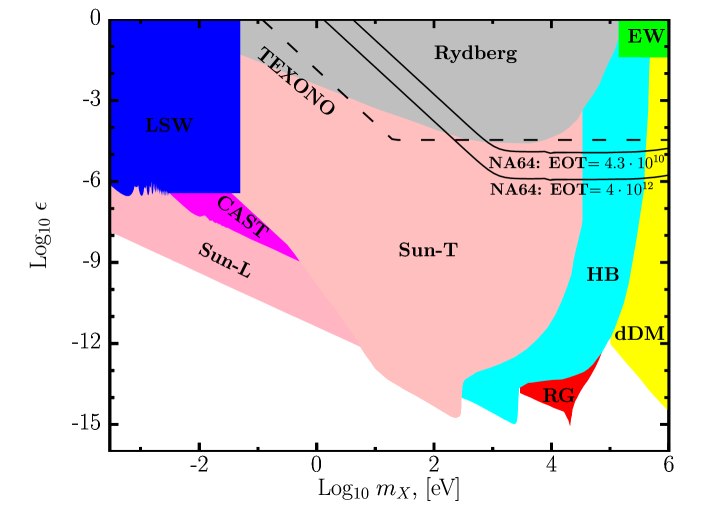
we present limits expected from the NA64 experiment on the model parameter space in the mass range 1 eV 1 MeV. The two NA64 limit curves obtained by making use of Eq. (51), refer to the statistics already collected by the experiment corresponding to electrons on target (EOT) Ref. [27] and to the ultimate statistics from the original proposal Ref. [16]. The mixing-independent horizontal parts match to the sensitivity lines presented in Ref [28] for keV, where the oscillation formalism we presented here reduces to the standard Compton-like description. At small masses the behaviour of the sensitivity limits matches Eq. (33). In Fig. 1 we also outline the exclusion regions evaluated from the results of the nuclear reactor experiment TEXONO [6], direct experimental searches (Rydberg, TEXONO, LSW, EW, and CAST) and disfavoured from the astrophysical considerations (HB, Solar Lifetime, dDM). For detailed discussion of various limits, see e.g. [6, 7, 29, 30]. One may argue that the bounds from stellar cooling are considerably more stringent than those from any expected direct searches. However, as we discussed in Introduction, results of the direct searches are much less sensitive to unknown systematics as compared to the astrophysical bounds which are typically not assumption-free. As an example, we point out that the Standard Solar Model, used to place the bounds presented in the Fig. 1, fails to simultaneously explain helioseismic data and photometric observables [31]. Unknown dynamics (including possible effect of new physics) behind this discrepancy could potentially change the solar bounds in Fig. 1. In addition, using the analysis of the light hidden photon production, propagation and detection developed in this work the future generation of the NA64-like experiments, such as e.g. eSPS/LDMX at the CERN SPS [32] which could potentially accumulate more than electrons on target, will be able to start direct probing the parameter space constrained from the astrophysical considerations with a much better sensitivity than NA64.
On the bright sight, there are two advantages inherent in the oscillation phenomenon. First, the probability to find a single photon in the detector generally exhibits a dependence on the distance covered by the oscillating state, see eq. (26), which can be exploited to suppress the background and/or distinguish the hidden-photon model from other SM extensions sharing the same signature. Moreover, this dependence provides a unique possibility to pin down the mass of the light hidden photon.
Second, the visible-to-hidden photon transition can be resonantly enhanced, provided by certain relations between the hidden photon mass , photon effective mass , absorption rate and energy :
| (41) |
Note, that in a given experiment, even if the energy of primary beam is too high to fulfill the inequality (41), there are less energetic particles emergent in the subsequent hadronic (electromagnetic) cascade, which can produce photons obeying (41). In particular, for the SHiP experiment, the relevant photon must come from rather soft, MeV pions. In the tungsten beam-dump these neutral pions decay into photons which conversion into the hidden photons of eV gets the resonance amplification.
The authors thank V. Duk, Yu. Kudenko and B. Kerbikov for useful discussions. The work is supported by the RSF grant 17-12-01547.
Appendix A Solution of the Schrodinger equation in homogeneous media
In a homogeneous media exact solution of the Schrodinger equation with the Hamiltonian (11) reads and can be explicitly written as
| (42) |
where
| (43) |
and are the Hamiltonian eigenvalues
| (44) |
This exact solution can be used for any set of the model and media parameters.
Appendix B Probability to produce the dark photon inside a sandwich-like structure
We calculate the probability to find the dark photon after a passage through a sandwich-like structure which is typical for electromagnetic calorimeters.
Let us assume, that the sandwich-like structure consists of two types of layers, of equal widths . One layer is assumed to be filled with some matter (e.g. lead) which is characterized by , while the other layer characterized by is filled with almost vacuum (scintillator), i.e. in this case.
Let us describe the evolution of wave function in each of the layers, numbered below by a subscript . We just make use of the solution (42) for each layer and properly combine them. Below we present the results up to corrections of order (or ).
| (45) |
see also Eq. (18). Here we introduced corresponding evolution matrices and for both types of layers.
Now let us find how the wave function of the system changes after passage through a single pair of layers. The propagation is described by the matrix , and we obtain
| (46) |
Here we made a simplification: in Eq. (46) we omitted a contribution proportional to in the “upper” element of the wave function as it is the second order in (remind that we are interested in the pure photon initial condition).
Now, having in mind the sandwich-like structure of the detector let us consider Eq. (46) as a recurrent relation of the following type
| (47) |
which relates the wave functions at boundaries of a single complex lead-scintillator layer (which actually consists of two elementary layers). Here
| (48) |
If we start with pure photon wave function, i.e. , then the asymptotic wave function is given by the following limit
| (49) |
with
| (50) |
We see that at the photon part of the wave function goes to zero, while the probability to find a dark photon is given by
| (51) |
One can easily check that if as expected. Then
| (52) |
where
| (53) | |||
| (54) | |||
| (55) | |||
| (56) |
and
| (57) |
This calculation assumes that the initial photon is produced at the left edge of a Pb-layer.
Let us introduce a correction related to the production position. We will assume that the photon is produced inside some Pb-layer, and in this first layer its path equals . The above formulas for evolution through the layers allow us to find the wave function after passage through the first pair of Pb (of length ) and vacuum (of length ) layers.
The propagation of the originally pure photon state in the part of the lead layer is described by the simplified matrix (45)
where is the penetration depth. For the propagation matrix one obtains
and if describes the state propagation through the vacuum layer of depth , then the propagation through a pair of lead and vacuum layers is described by . Now, we are interested to calculate
where , and is the depth of the photon production inside the lead layer. Then, at large
and hence
Then the probability of transition described by is
Let us remind again that here is the depth of the photon production inside the same lead production layer. At this expression turns into (51). This expression for the probability should be averaged (probably with MC simulations) over .
So the probability reads
where
and
Finally, we perform averaging over the scintillator layer by making use of the formulas
and find for the averaged probability
References
- [1] F. Vissani, Do experiments suggest a hierarchy problem?, Phys. Rev. D57 (1998) 7027–7030, [hep-ph/9709409].
- [2] G. F. Giudice, Naturalness after LHC8, PoS EPS-HEP2013 (2013) 163, [1307.7879].
- [3] M. Pospelov, A. Ritz and M. B. Voloshin, Secluded WIMP Dark Matter, Phys. Lett. B662 (2008) 53–61, [0711.4866].
- [4] P. Ilten, Y. Soreq, M. Williams and W. Xue, Serendipity in dark photon searches, JHEP 06 (2018) 004, [1801.04847].
- [5] M. Ahlers, H. Gies, J. Jaeckel, J. Redondo and A. Ringwald, Light from the hidden sector, Phys. Rev. D76 (2007) 115005, [0706.2836].
- [6] M. Danilov, S. Demidov and D. Gorbunov, Constraints on hidden photons produced in nuclear reactors, Phys. Rev. Lett. 122 (2019) 041801, [1804.10777].
- [7] J. Redondo and G. Raffelt, Solar constraints on hidden photons re-visited, JCAP 1308 (2013) 034, [1305.2920].
- [8] B. Kayser, On the Quantum Mechanics of Neutrino Oscillation, Phys. Rev. D24 (1981) 110.
- [9] E. Lifshitz and L. Pitaevski, vol. 10. Pergamon, Amsterdam, 1981.
- [10] E. Braaten and D. Segel, Neutrino energy loss from the plasma process at all temperatures and densities, Phys. Rev. D48 (1993) 1478–1491, [hep-ph/9302213].
- [11] G. G. Raffelt, Stars as laboratories for fundamental physics. 1996.
- [12] B. O. Kerbikov, The effect of collisions with the wall on neutron-antineutron transitions, 1810.02153.
- [13] J. Redondo, Atlas of solar hidden photon emission, JCAP 1507 (2015) 024, [1501.07292].
- [14] G. Raffelt and L. Stodolsky, Mixing of the Photon with Low Mass Particles, Phys. Rev. D37 (1988) 1237.
- [15] S. N. Gninenko, Search for MeV dark photons in a light-shining-through-walls experiment at CERN, Phys. Rev. D89 (2014) 075008, [1308.6521].
- [16] S. Andreas et al., Proposal for an Experiment to Search for Light Dark Matter at the SPS, 1312.3309.
- [17] J. L. Feng, I. Galon, F. Kling and S. Trojanowski, ForwArd Search ExpeRiment at the LHC, Phys. Rev. D97 (2018) 035001, [1708.09389].
- [18] FASER collaboration, A. Ariga et al., FASER’s Physics Reach for Long-Lived Particles, 1811.12522.
- [19] D. Curtin et al., Long-Lived Particles at the Energy Frontier: The MATHUSLA Physics Case, 1806.07396.
- [20] D. Curtin and M. E. Peskin, Analysis of Long Lived Particle Decays with the MATHUSLA Detector, Phys. Rev. D97 (2018) 015006, [1705.06327].
- [21] SHiP collaboration, M. Anelli et al., A facility to Search for Hidden Particles (SHiP) at the CERN SPS, 1504.04956.
- [22] S. Alekhin et al., A facility to Search for Hidden Particles at the CERN SPS: the SHiP physics case, Rept. Prog. Phys. 79 (2016) 124201, [1504.04855].
- [23] T2K collaboration, K. Abe et al., The T2K Experiment, Nucl. Instrum. Meth. A659 (2011) 106–135, [1106.1238].
- [24] DUNE collaboration, R. Acciarri et al., Long-Baseline Neutrino Facility (LBNF) and Deep Underground Neutrino Experiment (DUNE), 1601.05471.
- [25] DUNE collaboration, B. Abi et al., The DUNE Far Detector Interim Design Report Volume 1: Physics, Technology and Strategies, 1807.10334.
- [26] NA62 collaboration, E. Cortina Gil et al., The Beam and detector of the NA62 experiment at CERN, JINST 12 (2017) P05025, [1703.08501].
- [27] NA64 collaboration, D. Banerjee et al., Search for vector mediator of Dark Matter production in invisible decay mode, Phys. Rev. D97 (2018) 072002, [1710.00971].
- [28] S. N. Gninenko, D. V. Kirpichnikov, M. M. Kirsanov and N. V. Krasnikov, The exact tree-level calculation of the dark photon production in high-energy electron scattering at the CERN SPS, Phys. Lett. B782 (2018) 406–411, [1712.05706].
- [29] J. L. Hewett et al., Fundamental Physics at the Intensity Frontier, 1205.2671.
- [30] H. An, M. Pospelov, J. Pradler and A. Ritz, Direct Detection Constraints on Dark Photon Dark Matter, Phys. Lett. B747 (2015) 331–338, [1412.8378].
- [31] N. Vinyoles, A. M. Serenelli, F. L. Villante, S. Basu, J. Bergstrom, M. C. Gonzalez-Garcia et al., A new Generation of Standard Solar Models, Astrophys. J. 835 (2017) 202, [1611.09867].
- [32] T. Akesson, F. Bossi, A. Boveia, L. Bryngemark, M. Brugger, P. N. Burrows et al., Dark Sector Physics with a Primary Electron Beam Facility at CERN, Tech. Rep. CERN-SPSC-2018-023. SPSC-EOI-018, CERN, Geneva, Sep, 2018.