Existence of stationary fronts in a system of two coupled wave equations with spatial inhomogeneity

Abstract

We investigate the existence of stationary fronts in a coupled system of two sine-Gordon equations with a smooth, “hat-like” spatial inhomogeneity. The spatial inhomogeneity corresponds to a spatially dependent scaling of the sine-Gordon potential term. The uncoupled inhomogeneous sine-Gordon equation has stable stationary front solutions that persist in the coupled system. Carrying out a numerical investigation it is found that these inhomogeneous sine-Gordon fronts loose stability, provided the coupling between the two inhomogeneous sine-Gordon equations is strong enough, with new stable fronts bifurcating. In order to analytically study the bifurcating fronts, we first approximate the smooth spatial inhomogeneity by a piecewise constant function. With this approximation, we prove analytically the existence of a pitchfork bifurcation. To complete the argument, we prove that transverse fronts for a piecewise constant inhomogeneity persist for the smooth “hat-like” spatial inhomogeneity by introducing a fast-slow structure and using geometric singular perturbation theory.

1 Introduction

In this paper, we study the existence of front solutions in the following system of two spatially inhomogeneous sine-Gordon equations with coupling

$$\begin{split}\theta_{xx}-\theta_{tt}&=(1-d\rho(x))\sin\theta-\alpha\sin(\theta-\psi),\\ \psi_{xx}-\psi_{tt}&=(1-d\rho(x))\sin\psi-\alpha\sin(\psi-\theta),\end{split}$$ (1.1)

where $\theta=\theta(x,t),\psi=\psi(x,t)$, $\alpha\in\mathbb{R}$ is the coupling parameter and $d\in\mathbb{R}$ measures the strength of the spatial inhomogeneity $\rho(x).$ We consider the “hat-like” spatial inhomogeneity

$$\rho(x;\Delta,\delta):=\frac{\tanh((x+\Delta)/\delta)+\tanh((-x+\Delta)/\delta)}{2},$$ (1.2)

with $0<\delta\ll 1$, $\Delta>0$. Since $0<\delta\ll 1,$ apart from a small region near $|x|=\Delta$, the inhomogeneity is near zero for $|x|>\Delta$ and near 1 for $|x|<\Delta$; see Figure 1(a). Thus the variable $\Delta$ measures the half width of the $\rho(x;\Delta,\delta)$ “hat”. The small parameter $\delta$ determines the steepness of the inhomogeneity’s jump. As $\delta\to 0,$ $\rho(x;\Delta,\delta)$ converges pointwise to the piecewise constant function

$$\rho_{0}(x;\Delta)=\begin{cases}0,&|x|>\Delta,\\ 1,&|x|<\Delta,\end{cases}$$ (1.3)

(see Figure 1(b)) which will also be considered in this paper.

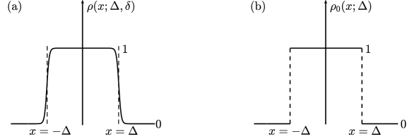
Figure 1: (a) is a sketch of the smooth “hat-like” spatial inhomogeneity $\rho(x;\Delta,\delta)$ whilst (b) is a sketch of the piecewise constant inhomogeneity $\rho_{0}(x;\Delta).$ Note the dashed lines correspond to $x=\pm\Delta,$ illustrating $\rho(\pm\Delta;\Delta,\delta)\approx 1/2.$

The coupled system (1.1) can be interpreted as a continuous approximation of two pendulum chains interacting with one another where the mass of the pendulums is allowed to change. The dependent variables $\theta$ and $\psi$ represent the angles of the two pendulum chains, the parameter $\alpha$ corresponds to the coupling strength between the two chains and the spatial inhomogeneity $\rho(x)$ represents a change in mass of the pendulums. The coupled system without spatial inhomogeneity $(d=0)$ was proposed as an elementary model for two parallel adatomic chains with small local interaction in [2]. Additionally the coupled system has been studied as a simple model of the DNA double helix [14, 20, 5], where the DNA chain is represented as a coupled pendulum chain. Furthermore, in the context of DNA it was proposed in [5], that the inhomogeneity $(d\neq 0)$ in the coupled system represents the presence of an RNA protein, an important mediator in DNA copying.

When $u(x,t)=\theta(x,t)=\psi(x,t)$ and $d=0$, the coupling and inhomogeneous terms in the system (1.1) vanish. As a result the system (1.1) reduces to the celebrated sine-Gordon equation [1, 9]

$$u_{xx}-u_{tt}=\sin(u).$$

The sine-Gordon equation is fully integrable and possesses a family of travelling front solutions

$$u_{\rm sG}^{\pm}(x,t;c)=4\arctan\bigg{(}\exp\bigg{(}\frac{\pm 1}{\sqrt{1-c^{2}}}{(x-ct+x^{*})}\bigg{)}\bigg{)},\quad|c|<1,\quad x^{*}\in\mathbb{R}.$$ (1.4)

Here $u_{\rm sG}^{+}$ represents the monotonic increasing front, whilst $u_{\rm sG}^{-}$ the monotonic decreasing one. Both fronts are centred at $x=-x^{*}$ when $t=0$ and move with constant speed $c.$ Thus when $c=0$ the fronts are stationary. Note that $u_{\rm sG}^{-}=2\pi-u_{\rm sG}^{+}$, which reflects the $u\mapsto 2\pi-u$ symmetry of the sine-Gordon equation.

From an application point-of-view, understanding front solutions and their dynamics is of special interest. Recent research into the interaction of travelling sine-Gordon fronts with finite length spatial inhomogeneities has produced fascinating results. In [19] Piette and Zakrzewski studied the scattering of (1.4) in the inhomogeneous sine-Gordon equation

$$u_{xx}-u_{tt}=(1-d\rho_{0}(x;\Delta))\sin(u)$$ (1.5)

with the piecewise constant spatial inhomogeneity (1.3). Starting the travelling front far away from the inhomogeneity they noted several different phenomena dependent on the initial speed and $d,\Delta.$ Fix $d,\Delta>0$, then for values of $c$ less than some critical one the travelling front would not pass and get stuck in the inhomogeneity. For higher speeds the front could pass through the inhomogeneity. Interestingly they noted some speed values less than the critical one that fronts could bounce back out of the inhomogeneity. More recently, Goatham et al. studied the scattering of the travelling sine-Gordon fronts (1.4) in (1.5) with smooth non-steep spatial inhomogeneities; see [10].

It has also been shown the existence of stationary fronts plays a role in studying the interaction of travelling fronts with spatial inhomogeneities [4]. This is because stationary front solutions correspond to fixed points in the dynamical systems approach to the wave equation. The existence of stationary front solutions to the inhomogeneous sine-Gordon equation (1.5), with boundary conditions $u(-\infty)=0$ and $u(+\infty)=2\pi,$ for all $d\in\mathbb{R}$ and $\Delta>0$ was established in [4]. We denote these fronts by $u_{0}(x;d,\Delta)$, hence $u_{0}(x;d=0,\Delta)=u_{\rm sG}^{+}(x,t;0)$. In the special case, $d=1$, Derks et al. [4] also gave the explicit expression for the front solutions,

$$u_{0}(x;d=1,\Delta)=\begin{cases}4\arctan(e^{x+x^{*}}),&x<-\Delta\\ \pi+\sqrt{2h}x,&|x|<\Delta\\ 4\arctan(e^{x-x^{*}}),&x>\Delta,\end{cases}$$ (1.6)

where $0<h(\Delta)<2$ is uniquely determined by

$$\Delta=\arccos(h-1)/\sqrt{2h}\quad\mbox{and}\quad x^{*}=\ln(\tan(\arccos(1-h)/4))+\Delta.$$ (1.7)

These solutions persist in the coupled system (1.1) when $\delta=0$.

Returning to the full coupled system (1.1), when there is no spatial inhomogeneity, i.e. $d=0$, the sine-Gordon fronts $\theta(x,t)=\psi(x,t)=u_{\rm sG}^{\pm}(x,t;c)$ are stable if $-1/2<\alpha<0$ and unstable if $0<\alpha<1/2;$ see [2]. We illustrate this instability for the stationary front $u_{\rm sG}^{+}(x,t;0)$ in a numerical time simulation of (1.1) with $d=0$ and $\alpha=0.1$ in Figure 2(a). The instability manifests itself by the stationary fronts travelling apart. We now consider a numerical time simulation of the stationary front $u_{\rm sG}^{+}(x,t;0)$ in (1.1) when $d\neq 0;$ see Figure 2(b-c). Fixing $0<\delta\ll 1,d>0$ and $\Delta>0$ the stationary fronts with $\theta=\psi=u_{\rm sG}^{+}$ first adapt themselves to account for the presence of a spatial inhomogeneity then two different phenomena can occur. For small values of $\alpha>0$ the stationary fronts are stable; see Figure 2(b). On the other hand, for larger values of $\alpha<1/2$ the stationary fronts are unstable and bifurcate to new stationary fronts with $\theta\neq\psi$; see Figure 2(c). When plotting in the coordinates

$$u=\frac{\theta+\psi}{2}\quad\mbox{and}\quad v=\frac{\theta-\psi}{2}$$ (1.8)

one starts to see how this bifurcation occurs. The case $\theta(x)=\psi(x)$ in the original variables corresponds to $(u(x),v(x))=(\theta(x),0)$ in the new ones. For fixed $d>0,$ we see in Figure 2(b) that for small values of $\alpha$, $(u(x),v(x))=(\theta(x),0)$ is stable, i.e. the inhomogeneity has stabilized the sine-Gordon front in the coupled system. For larger values of $\alpha$, Figure 2(c) shows that a bifurcation has happened: the effect of the coupling initially dominates the stabilizing effect of the inhomogeneity and the $\theta$ and $\psi$ components start to travel apart as in (a), but soon afterwards, the inhomogeneity dominates again and the fronts get stopped. This results in $v$ becoming a small localised pulse.

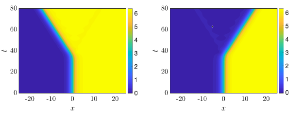
(a) (a)

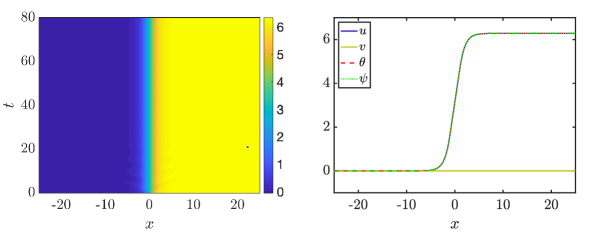
(b) (b)

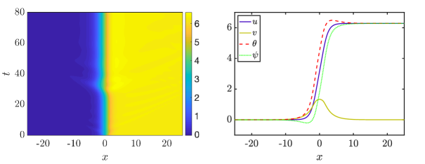
(c) (c)

Figure 2: (a) corresponds to space-time plots of the dynamics of the initial condition consisting of the stationary sine-Gordon front solutions in the system (1.1) with $\alpha=0.1$ and no spatial inhomogeneity, i.e. $d=0$. The left panel corresponds to $\theta(x,t)$ and the right $\psi(x,t)$. After a while, the fronts loose stability and begin to travel apart. The left panel of (b) correspond to a space-time plot of the $\theta(x,t)$ dynamics of the same initial condition, now with the spatial inhomogeneity $\delta=1/15$ and $\Delta=d=1$, while keeping $\alpha=0.1$. The right panel corresponds to the solution profile at $t=80$. The left panel of (c) corresponds to a space-time plot of the $\theta(x,t)$ dynamics, again with the same initial condition, now for a stronger coupling $\alpha=0.4$, and the same inhomogeneity $\delta=1/15$ and $\Delta=d=1$. The right panel corresponds to the solution profile at $t=80.$ Note that as we are interested in stationary solutions a small damping term was added in (b) and (c) to suppress the additional radiation generated by the initial adaptation in the Hamiltonian system.

The main aim of this paper is to provide a detailed numerical and analytical understanding of the bifurcation shown in Figure (2)(b-c). We will do this by studying the existence of stationary fronts to the coupled system (1.1) when $0<\alpha<1/2$, $d>0$, $\Delta>0$ and $0\leqslant\delta\ll 1$. The restriction on $\alpha$ is due to the fact that the steady state $(\theta,\psi)=(2\pi,2\pi)$ is temporally unstable for $\alpha>1/2$. Note that the $\delta=0$ case corresponds to the piecewise constant inhomogeneity, i.e. $\rho(x)=\rho_{0}(x;\Delta)$ given by (1.3). Since the sine-Gordon symmetry persists for the full coupled system (1.1) we can restrict ourselves to the monotonic increasing fronts. It is helpful to keep the change of variables (1.8). Consequently, the existence of stationary front solutions in the coupled inhomogeneous system (1.1) is equivalent to the existence of solutions to the Boundary Value Problem (BVP)

$$\begin{split}u_{xx}&=(1-d\rho(x))\sin u\cos v,\\ v_{xx}&=(1-d\rho(x))\sin v\cos u-\alpha\sin 2v.\end{split}$$ (1.9)

$$\lim_{x\to-\infty}(u(x),v(x))=(0,0)\quad\text{and}\quad\lim_{x\to+\infty}(u(x),v(x))=(2\pi,0).$$ (1.10)

When $v(x)=0,$ the system (1.9) reduces to the stationary inhomogeneous sine-Gordon equation

$$u_{xx}=(1-d\rho(x))\sin u,\quad\lim_{x\to-\infty}u(x)=0\quad\text{and}\quad\lim_{x\to\infty}u(x)=2\pi.$$ (1.11)

An obvious starting point for the analysis to understand the bifurcation occurring in Figure 2 is to build on the work on the uncoupled inhomogeneous sine Gordon equation in [4] and consider the case $d=1$, $\delta=0$ (the piecewise constant inhomogeneity $\rho_{0}(x;\Delta)$ given by (1.3)) and carry out a Lyapunov-Schmidt reduction analysis for the explicit front solution (1.6). As the front is a non-constant state, this poses some challenges to be overcome. The next step would be to extend the existence for the piecewise constant inhomogeneity $\rho_{0}(x;\Delta)$ to the smooth inhomogeneity $\rho(x;\Delta,\delta)$ (1.2). Whilst for fixed $\Delta$ the function $\rho(x;\Delta,\delta)$ converges pointwise to $\rho_{0}(x;\Delta)$ as $\delta\to 0$, the link between the front (1.6) and front solutions in (1.1) is not immediately obvious.

In order to overcome this issue, we adapt an approach by Goh and Scheel [11]. They study fronts in the complex Ginzburg-Landau equation with a smooth single step inhomogeneity and characterise this inhomogeneity with an additional Ordinary Differential Equation (ODE). Following this approach, we extend the coupled system with the following additional ODE for the inhomogeneity $\rho$:

$$\delta^{2}\rho_{xx}=4\rho^{3}-(6+4\epsilon)\rho^{2}+2(1+\epsilon)\rho.$$

When $0<\epsilon,\delta\ll 1$, this ODE has explicit solutions where (1.2) is the leading order approximation and $\epsilon$ can be expressed in terms of $\Delta$ and $\delta$ ($\epsilon=\mathcal{O}(e^{-2\sqrt{2}\Delta/\delta})$). Including this ODE in the system (1.9) turns the problem into a fast-slow dynamical system where geometric singular perturbation theory can be applied and existence of solutions can be proved for fixed $\Delta$ and $0<\delta\ll 1$. The key part of the geometric singular perturbation theory is to understand the singular limit $\delta\to 0$, where $\rho$ is determined by an algebraic equation, then use Fenichel’s theorems [8] to prove persistence when $0<\delta\ll 1.$

We have four main results. The first is a systematic numerical investigation of the bifurcation illustrated in Figure 2(b–c) using numerical path following in the $(\alpha,d,\Delta)$ parameter space. In particular, this numerical investigation allows us to explore several limiting cases where analysis is possible. With this analysis, we obtain two theorems about the location of the bifurcation from the sine-Gordon front and the emerging bifurcating states using the piecewise constant $\rho_{0}(x;\Delta)$ (1.3). Finally, we prove that the fronts found for a piecewise constant inhomogeneity $\rho_{0}(x;\Delta)$ persist for the smooth inhomogeneity $\rho(x;\Delta,\delta)$ (1.2) for $0<\delta\ll 1$.

The structure of this paper is as follows. Section 2 presents a numerical investigation into the BVP (1.9-1.10). Starting with a solution of the form $(u(x),v(x))=(u(x),0)$, we show the existence of a pitchfork bifurcation at which $v(x)$ becomes non-zero in the parameter space with $\alpha\in(0,1/2)$ and $d,\,\Delta>0$. In Section 3 we use the piecewise constant inhomogeneity $\rho_{0}(x;\Delta)$ to determine an analytical expression for the bifurcation locus in case $d=1$ and derive approximations for the bifurcation locus observed in Section 2 in the cases $d$ large and $\Delta$ large. Using the bifurcation locus expression and the front solution (1.6), we employ Lyapunov-Schmidt reduction to show the existence of a pitchfork bifurcation and approximate the bifurcating solutions in Section 4 for the case $d=1$. In Section 5 we use regular and singular perturbation theory to show that if solutions exist with the inhomogeneity $\rho_{0}(x;\Delta)$, then they persist for the smooth inhomogeneity $\rho(x;\Delta,\delta).$ This result rigorously justifies comparisons between the numerics and the analysis made throughout the paper. Finally, in Section 6 we end with a summary of the main results and a discussion of further research.

2 Numerical bifurcation investigation

In this section we numerically investigate a bifurcation in the inhomogeneous coupled sine-Gordon BVP (1.9-1.10) from the solution state $(u(x),v(x))=(u(x),0)$ to one where $v(x)\neq 0$. Recall (1.9) has four parameters: the coupling parameter $\alpha$, the strength of the inhomogeneity $d$, the steepness $\delta$ and the width $\Delta$. Throughout this section we keep the steepness parameter $\delta=1/15$ fixed. First fixing $d=\Delta=1$, we determine a bifurcation point in the remaining parameter $\alpha$ whereby $v(x)$ undergoes a pitchfork bifurcation. After this, we keep $d=1$ fixed but consider any $\Delta>0$ and plot the corresponding bifurcation diagram in the $(\alpha,\Delta)$ plane. We finish this section by showing the pitchfork bifurcation occurs for any $d>0$ and give plots in the $(d,\Delta)$ plane for various fixed values of $\alpha\in(0,1/2)$, illustrating the existence of a two dimensional bifurcation manifold in the $(\alpha,d,\Delta)$ parameter space.

To start this numerical bifurcation section, we discuss how to set up the problem for numerical investigation.

2.1 Implementation

We will study the BVP (1.9-1.10) using AUTO07p [6]. AUTO07p requires us to re-write (1.9) as a first order ODE system. Hence we consider

$$u_{x} =p,$$

$$p_{x} =(1-d\rho(x;\Delta,\delta))\sin u\cos v,$$

$$v_{x} =q,$$ (2.1)

$$q_{x} =(1-d\rho(x;\Delta,\delta))\sin v\cos u-\alpha\sin 2v,$$

where the smooth inhomogeneity $\rho(x;\Delta,\delta)$ is defined in (1.2). Note that AUTO07p is unable to deal with the piecewise constant approximation $\rho_{0}(x;\Delta)$ of $\rho(x;\Delta,\delta)$. The dynamics of (2.1) are centred at $x=0$ however AUTO07p requires us to consider the dynamics on a positive spatial interval. Thus we apply the spatial translation $\tilde{x}=x+50$ to (2.1) which centres the dynamics at $\tilde{x}=50.$ We consider the dynamics over the finite interval $\tilde{x}\in[0,100]$ with boundary conditions $(u,p,v,q)(\tilde{x}=0)=(0,0,0,0)$ and $(u,p,v,q)(\tilde{x}=100)=(2\pi,0,0,0).$ When plotting the data we have reverted the shift transformation (consider $x=\tilde{x}-50$) so that it is once again centred at $x=0$ and satisfies (2.1). Due to the spatial inhomogeneity no phase condition is needed. Finally, we use standard AUTO07p tolerances as detailed in [6].

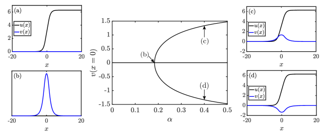
Figure 3: A plot of the bifurcation branches and evolution of $v(x)$ solution in the system (2.1) with $d=1=\Delta$ and varying $\alpha\in(0,1/2)$. Panel (a) corresponds to the solution with $v(x)=0$ which exists for all $\alpha\in(0,1/2)$. The bifurcation locus is at $\alpha\approx 0.18$. Panel (b) shows the $u$ (black) and $v$ (blue) eigenfunctions with the eigenvalue 0 respectively. Panel (c) displays the $u$ and $v$ components of the solution on the positive bifurcation branch at $\alpha=0.4$. Panel (d) displays the $u$ and $v$ components of the solution on the negative bifurcation branch at $\alpha=0.4$.

2.2 The bifurcation when $\bm{d=1}$

Consider $d=1.$ Then, in the limit $\delta\to 0,$ it follows from [4] that for any $\Delta>0$, the system (2.1) has stationary front solutions $(u(x),u_{x}(x),0,0)$ with $u(x)$ given by (1.6). When $0<\delta\ll 1,$ AUTO07p shows that there are nearby stationary solutions of (2.1) that satisfy the boundary conditions $u(x=-50)=0$ and $u(x=50)=2\pi$. Considering $\Delta$ fixed and varying $\alpha\in(0,1/2)$, one can find a pitchfork bifurcation point at some $\alpha=\alpha^{*}$ whereby the $(v,q)$ component can become non-zero. For example, fixing $\Delta=1$ we find a pitchfork bifurcation at $\alpha^{*}\approx 0.18$. Figure 3 shows this bifurcation for $\Delta=1$ and the new emerging branches where $v(x)$ is non-zero in the region $\alpha\in(0,1/2)$. Figure 3(a-b) show the $u$ and $v$ components of the solution and the eigenfunctions for the zero eigenvalue, respectively, at the bifurcation point $\alpha^{*}\approx 0.18$. In particular, we see that the eigenfunction for the $u$ component is zero whereas for the $v$ component it is a localised function. Fixing $\alpha=0.4>\alpha^{*}$, the $u$ and $v$ components of the solution on the positive and negative branches of the system (2.1), with $d=1$ and $\Delta=1$, are plotted in Figures 3(c) and 3(d) respectively. Here we observe the emergence of a localised $v$ component that steadily grows as we move away from the bifurcation point.

In Figure 4 we trace out the locus of the pitchfork bifurcation point $\alpha^{*}(\Delta)$ in the $(\alpha,\Delta)$ plane. For parameters $(\alpha,\Delta)$ chosen on the right side of the bifurcation diagram there exists non-zero $v(x)$ solutions. Whilst on the left only solutions with $v=0$ exist. This figure shows that the largest value of $\alpha$ that the pitchfork bifurcation can occur is $\alpha^{*}\approx 0.185$. Hence, when $d=1$, the bifurcation occurs when the coupling between $u(x)$ and $v(x)$ components is small.

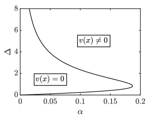
Figure 4: The locus of the pitchfork bifurcation in the $(\alpha,\Delta)$ plane when $d=1$. The $v(x)=0$ solution exists for all parameter choices but for choices on the right of the curve $v(x)\neq 0$ solutions also exist.

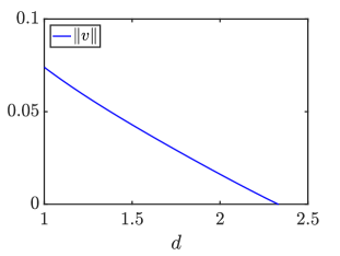
(a)

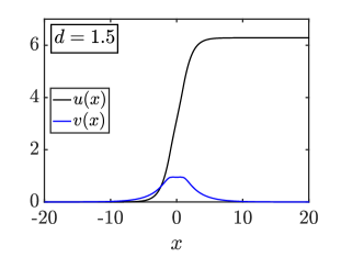
(b)

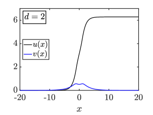
(c)

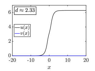
(d)

Figure 5: The top left panel shows the evolution of the $L^{2}$ norm of non-zero $v(x)$ component for $d\in[1,2.33]$ where $\alpha=0.4$ and $\Delta=1.$ The other panels show snapshots $u$ and $v$ components of the solution, for different values of $d$, of the system (2.1). This illustrates that the $v$ component shrinks as $d$ increases.

2.3 The bifurcation for any $\bm{d>0}$

We now show the pitchfork bifurcation occurs for any $d>0$. Consider the solution with $v(x)\neq 0$ in Figure 3(c) with fixed $\alpha=0.4$, $\Delta=1$, and $d=1$. Increasing the parameter $d$ results in the decay of the $v(x)$ component of the solution; see Figure 5. Notice that when $d\neq 1$ the $v(x)$ solution does not always have a bell shape; Figure 5 shows the $v(x)$ component developing two maximum points as $d$ increases. Eventually, at $d\approx 2.33$ the $v(x)$ component vanishes. This implies that, when $\Delta=1$, the bifurcation point $\alpha^{*}\approx 0.185$ observed for $d=1$ increases to $\alpha^{*}=0.4$ as $d$ increases to $d\approx 2.33$. Figure 6(a) shows this behaviour happens for all $\Delta$. It shows the bifurcation locus in the $(\alpha,\Delta)$ plane for $d=2.33,d=1$ and $d=0.5.$ For parameter choices to the left of the bifurcation loci, only solutions with $v(x)=0$ exist whilst for parameters selected on the right of the curves there are also solutions with a non-zero $v$ component. As $d$ increases, the locus moves rightwards and the solution with $v(x)=0$ becomes the dominant one since there is less parameter choice for the solution with $v(x)\neq 0$ to exist. On the other hand, as $d$ decreases the curve moves leftwards and more solutions with $v(x)\neq 0$ exist. In particular, for $d<1$, the loci asymptote to $\alpha=0$ for $\Delta\to\infty$ and are also close to $\alpha=0$ for a large range of $\Delta$ values. In Figure 6(b) we plot the bifurcation branches for the $v(x)$ component when $d\approx 2.33$ and $\Delta=1$.

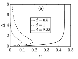
(a)

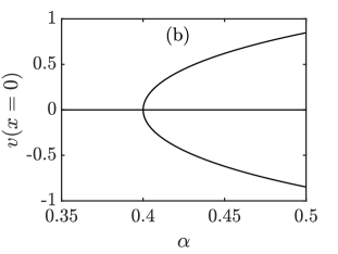
(b)

Figure 6: Panel (a) corresponds to the bifurcation locus in the $(\alpha,\Delta)$ plane when $d=0.5$, $1$, and $2.33$. To the right of each curve $v(x)\neq 0$ solutions exist. Panel (b) shows the bifurcation branches and the evolution of the $v(x)$ solution when $\Delta=1$ and $d=2.33$.

Finally we fix $\alpha$ and consider the bifurcation locus in the $(d,\Delta)$ plane. In the main panel of Figure 7 we trace the pitchfork bifurcation locus in the $(d,\Delta)$ plane for fixed $\alpha=0.4$. On the curve and in the area to the right $v(x)=0$. Meanwhile on the left $v(x)\neq 0$ solutions also exist. Figures 7(a-c) give details about the solution ($u(x)$ and $v(x)$ components and $(u,p)$ phase plane, where $p=u_{x}$, and eigenfunction for the eigenvalue zero at selected points on the curve. Figure 7(a) corresponds to a large $\Delta$ value at the top of the curve ($\Delta=8$). Here we observe that the $u$ front has a plateau around $\pi$ at $x=0$. As one passes to the points (b) and (c) on the curve in Figure 7 (hence $\Delta$ decreases and $d$ increases), we see that this plateau disappears and $u$ tends to the unperturbed sine-Gordon front as $d$ becomes large.

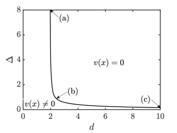
(a)

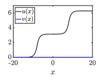
(b)

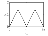
(c) (a)

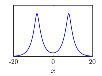
(d)

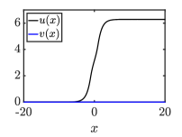
(e)

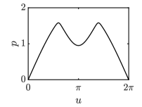
(f) (b)

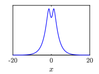
(g)

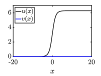
(h)

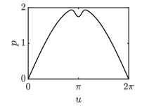
(i) (c)

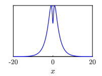
(j)

Figure 7: The top panel shows the bifurcation locus for $\alpha=0.4$ in the $(d,\Delta)$ plane. Panels (a), (b), and (c) give details at the three bifurcation points labelled in the top panel. The left column represents the physical space whilst the middle is a plot of the $(u,p)$ phase space, where $p=u_{x}$. The final column is a plot of the $v$ component of the eigenfunction at the eigenvalue zero.

In Figure 8(a), bifurcation loci in the $(d,\Delta)$ parameter plane have been plotted for $\alpha=0.01$, $0.1$, $0.25$, $0.4$, and $0.49$. To the right of each curve $v(x)=0$ is the only solution whilst to the left non-zero solutions for $v(x)$ exist. As $\alpha\to 1/2$, the bifurcation locus translates rightwards and more $v(x)\neq 0$ solutions exist. On the other hand as $\alpha\to 0$ the locus moves leftwards and becomes non-monotonic. However for fixed values of $\Delta$, the curves have the property that $d\to 0$ as $\alpha\to 0$. Also, for $\alpha$ fixed, the bifurcation curves asymptote to $\Delta=0$ for $d\to\infty$ and to some $d(\alpha)>1$ for $\Delta\to\infty$, with $d(\alpha)\to 1$ for $\alpha\to 0$. This is illustrated in Figure 8(b) where the bifurcation locus in the $(\alpha,d)$ parameter plane is shown for fixed $\Delta=8$ and $0.01\leqslant\alpha\leqslant 0.49$.

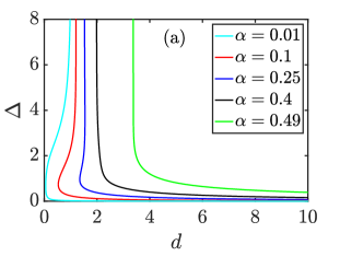
(a)

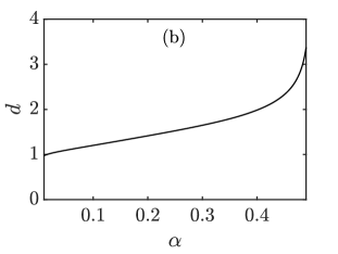
(b)

Figure 8: (a) shows the bifurcation locus in the $(d,\Delta)$ plane for several fixed values of $\alpha$. (b) gives the bifurcation locus in the $(\alpha,d)$ plane for fixed $\Delta=8$ and $\alpha\in[0.01,0.49]$.

3 Bifurcation manifold analysis

Upon fixing $0<\delta\ll 1$, the numerical investigation in the previous section on the BVP (1.9-1.10) suggests that there is a single bifurcation manifold in the three parameter space $(\alpha,d,\Delta)$ where a pitchfork bifurcation occurs. On this manifold the solution state $(u(x),v(x))=(u(x),0)$ bifurcates to one where $v(x)\neq 0$.

Using the piecewise constant inhomogeneity $\rho_{0}(x;\Delta)$ given in (1.3) we have the explicit expression (1.6) for solutions $(u(x),v(x))=(u_{0}(x;d,\Delta),0)$ to the BVP (1.9-1.10) in the $d=1$ case. Furthermore, we can derive approximations for the solutions $u_{0}(x;d,\Delta)$ in the $d\gg 1$ and $\Delta\gg 1$ limits. So in this section we consider the piecewise constant inhomogeneity $\rho_{0}(x;\Delta)$ as an approximation of $\rho(x;\Delta,\delta)$. We look for the critical parameters in the three parameter space $(\alpha,d,\Delta)$ of the BVP

$$\begin{split}u_{xx}&=(1-d\rho_{0}(x;\Delta))\sin u\cos v,\\ v_{xx}&=(1-d\rho_{0}(x;\Delta))\sin v\cos u-\alpha\sin 2v,\end{split}$$ (3.1)

$$\lim_{x\to-\infty}(u(x),v(x))=(0,0)\quad\text{and}\quad\lim_{x\to+\infty}(u(x),v(x))=(2\pi,0),$$ (3.2)

at which the solution state $(u(x),v(x))=(u_{0}(x;d,\Delta),0)$ can bifurcate to one where $v(x)\neq 0$. To be specific, we find the parameter values for which the linearisation about the state $(u_{0}(x;d,\Delta),0)$ has an eigenvalue zero. When $d=1$ we determine an implicit relation between $\alpha$ and $\Delta$ that characterises the bifurcation locus. When $d\gg 1$ or $\Delta\gg 1$, we obtain approximations of the bifurcation locus. We give these results in the following Theorem.

Theorem 1

Consider the BVP (3.1-3.2). In the cases below, the solution $(u(x),v(x))=(u_{0}(x;d,\Delta),0)$ can bifurcate to a solution with $v\neq 0$.

Case 1: $\bm{d=1}$

The bifurcation locus $\alpha(\Delta)$ is determined implicitly by

$$\frac{h}{2}-\sqrt{1-2\alpha}\bigg{(}\sqrt{1-2\alpha}+\frac{\sqrt{2(2-h)}}{2}\bigg{)}\\ =-\sqrt{2\alpha}\bigg{(}\sqrt{1-2\alpha}+\frac{\sqrt{2(2-h)}}{2}\bigg{)}\tan\bigg{(}\sqrt{\frac{\alpha}{h}}\bigg{(}\arccos(h-1)\bigg{)}\bigg{)}$$ (3.3)

where $0<h<2$ is determined from the one to one relation $\Delta=\arccos(h-1)/\sqrt{2h}$.

Case 2: $\bm{d\gg 1}$

For $0<\alpha<1/2$ the bifurcation locus is approximated by

$$\Delta(\alpha;d)=\frac{1}{d}\bigg{(}\frac{2\alpha}{\sqrt{1-2\alpha}}\bigg{)}\bigg{(}1+\mathcal{O}\bigg{(}\frac{1}{\sqrt{d}}\bigg{)}\bigg{)}.$$ (3.4)

Case 3: $\bm{\Delta\gg 1}$

1. When $d>1$ the bifurcation locus is approximated by $\alpha(d;\Delta)=\alpha_{0}(d)+\mathcal{O}(e^{-\sqrt{d-1}\Delta})$ with $\alpha_{0}(d)$ the solution of

   $$\left(\frac{\sqrt{1-2\alpha_{0}}}{\sqrt{d}}-2\alpha_{0}+\frac{1}{d}\right)\left(\frac{d-1}{\sqrt{d}}+\sqrt{d-1-2\alpha_{0}}\right)\\ +\left(\frac{1}{\sqrt{d}}+\sqrt{1-2\alpha_{0}}\right)\left(\frac{d-1}{\sqrt{d}}\sqrt{d-1-2\alpha_{0}}-{2\alpha_{0}}+\frac{(d-1)^{2}}{d}\right)=0.$$ (3.5)

   This implies that $0\leqslant\alpha_{0}(d)<\frac{1}{2}\min(d-1,1)$ and $\alpha_{0}(d)=\frac{d-1}{2}+\mathcal{O}((d-1)^{2})$ for $d\downarrow 1$.

2. When $0<d<1$ the bifurcation locus satisfies $\alpha(d;\Delta)=o(1)$ for $\Delta\to\infty$.

The bifurcation locus $\alpha(\Delta)$ in case 1 can not be distinguished from the numerics shown in Figure 4. The approximations of the bifurcation locus in cases $2$ and $3(a)$ are plotted in Figure 9 and compared with the numerically computed ones seen in the previous section. Here we see excellent agreement in the respective limits for $d\to\infty$ and for $\Delta\to\infty$ with $d>1$. For fixed $0<d<1$, case $3(b)$ clarifies the numerical results in Figure 6(a) (where $d=0.5$) and the sharp downturn in the $d(\alpha)$ curve in Figure 8(b).

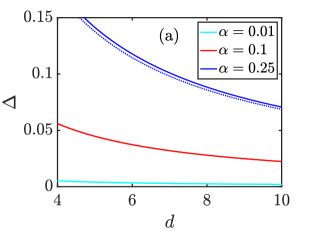
(a)

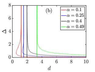
(b)

Figure 9: The solid curves in (a) shows the approximation (3.4) of the bifurcation locus in the $(d,\Delta)$ plane for fixed $\alpha$ and large $d.$ The solid lines in (b) shows the approximation (3.5) of the bifurcation locus for fixed $\alpha$ and large $\Delta.$ In both (a) and (b) the dashed curves correspond to the numerics presented in the previous section.

The remainder of this section is spent proving this theorem. First we consider the solutions of the BVP (3.1-3.2) with $v(x)=0$. When $v(x)=0$, the BVP reduces to,

$$u_{xx}=(1-d\rho_{0}(x;\Delta))\sin u$$ (3.6)

$$\lim_{x\to-\infty}u(x)=0\quad\text{and}\quad\lim_{x\to+\infty}u(x)=2\pi.$$ (3.7)

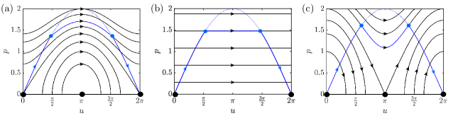
Figure 10: The black trajectories in (a), (b) and (c) correspond to solution curves in the phase plane of $H_{1}$ (see (3.9)) for $d=0.5$, $d=1$ and $d=2$ respectively. In each panel, the dashed blue curve is the heteroclinic connection in the $H_{0}$ dynamics (see (3.8)) and the bold blue curve corresponds to front solutions of (3.6) with $\Delta=1$. Finally the blue points represent the matching points (3.10).

We call (3.6) the inhomogeneous sine-Gordon equation. The existence of fronts that connect $u=0$ to $u=2\pi$ for all $d\in\mathbb{R}$ and $\Delta>0$ is shown in [4]. The construction used in this paper is based on the following idea which is illustrated in Figure 10. Since the spatial inhomogeneity is piecewise constant, we can interpret (3.6) as a homogeneous Hamiltonian system in both individual regions $|x|>\Delta$ and $|x|<\Delta$.

The Hamiltonian of (3.6) in the region $|x|>\Delta,$ i.e. when $\rho_{0}=0$, is

$$H_{0}(u,p)=\frac{1}{2}p^{2}+\cos(u)-1,$$ (3.8)

with $p=u_{x}$. The Hamiltonian is chosen such that it vanishes on the heteroclinic connection between $(0,0)$ and $(2\pi,0)$. This heteroclinic connection corresponds to the stationary sine-Gordon front, i.e. $u_{sG}^{+}$ in (1.4) with $c=0$, and is explicitly described by

$$\left(\begin{array}[]{c}u(x)\\ p(x)\end{array}\right)=\left(\begin{array}[]{c}4\arctan(e^{x+x^{*}})\\ 2\operatorname{sech}(x+x^{*})\end{array}\right),\quad\text{where}\quad x^{*}\in\mathbb{R}.$$

The front solution to the inhomogeneous sine-Gordon equation has to lie on this heteroclinic connection for $|x|>\Delta$, hence the solution has to satisfy $H_{0}(u(x),p(x))=0$ for $|x|>\Delta$.

On the other hand, in the region $|x|<\Delta,$ i.e. when $\rho_{0}=1,$ the Hamiltonian is

$$H_{1}(u,p)=\frac{1}{2}p^{2}+(1-d)(1+\cos(u)),$$ (3.9)

with $p=u_{x}$. This Hamiltonian is chosen such that it vanishes on the fixed point $(u,p)=(\pi,0)$. This fixed point is a saddle point when $d>1$ and a centre when $d<1.$ A front solution of the inhomogeneous sine-Gordon equation can be characterised by the value of the Hamiltonian $H_{1}$ on the interval $|x|<\Delta$. Denote this value by $h$. Then a front solution $u(x)$ of (3.6) satisfies $H_{1}(u(x),p(x))=h$ with $h>0$ for $|x|<\Delta$. The relations $H_{0}=0$ and $H_{1}=h$ at $x=-\Delta$ give the following matching coordinates

$$u^{-}(h;d):=u(-\Delta)=\arccos\left(-1+\frac{2-h}{d}\right)\quad\text{and}\quad p^{-}(h;d):=p(-\Delta)=\sqrt{\frac{4(d-1)+2h}{d}}.$$ (3.10)

Furthermore we have the following symmetry relations $u^{+}=2\pi-u^{-}$ and $p^{+}=p^{-}.$ It can be seen from (3.10) that both $u^{-}$ and $p^{-}$ are increasing in $h$ and $(u^{-},p^{-})\to(\pi,2)$ as $h\to 2$. Consequently the values of the Hamiltonian $H_{1}$ relevant for the construction of a stationary front are $0<h\leqslant 2$. Finally, the Hamiltonian $H_{1}$ can be used to derive a bijection between the length of the inhomogeneity $\Delta>0$ and the parameter $h\in(0,2)$, thus $h$ can be considered as a function of $\Delta$.

When $d=1$, the non-linearity in (3.6) vanishes in the region $|x|<\Delta$ and the construction can be used to show that the fronts are given explicitly by (1.6). When $d\neq 1$, it is no longer possible to construct explicit fronts without employing the Jacobi elliptic functions. However, the construction above can be used to show that the front is close to $\pi$ for all $|x|<\Delta$ when $d\gg 1$ and also that its shape for $|x|<\Delta$ is close to the sine-Gordon front shape $u_{\rm sG}^{+}$ when $\Delta\gg 1$.

Next we return to the full BVP (3.1-3.2). We set $\bm{w}=(u,v)$ and hence consider boundary conditions $\bm{w}(-\infty)=(0,0)$ and $\bm{w}(+\infty)=(2\pi,0)$. We denote the front solution of the inhomogeneous sine-Gordon equation as constructed above by $u_{0}(x;d,\Delta)$. Then $\bm{w}_{0}=(u_{0},0)$ solves (3.1) for all $\alpha\in\mathbb{R}.$ We wish to determine the bifurcation points in the three parameter space at which the second component becomes non-zero. Due to the non-zero boundary conditions, it is convenient to set

$$\bm{\tilde{w}}=\bm{w}-\bm{w_{0}}\in H^{2}(\mathbb{R})\times H^{2}(\mathbb{R}).$$

Now, fixing $d,\Delta>0$, we can define $\mathbf{{F}}:H^{2}(\mathbb{R})\times H^{2}(\mathbb{R})\times\mathbb{R}\mapsto L^{2}(\mathbb{R})\times L^{2}(\mathbb{R})$ where

$$\mathbf{{F}}(\bm{\tilde{w}};\alpha)=\left(\begin{array}[]{ c }\tilde{u}_{xx}\\ \tilde{v}_{xx}\end{array}\right)-\left(\begin{array}[]{ c }(1-d\rho_{0})(\sin(\tilde{u}+u_{0})\cos(\tilde{v})-\sin(u_{0}))\\ (1-d\rho_{0})\sin(\tilde{v})\cos(\tilde{u}+u_{0})-\alpha\sin(2\tilde{v})\end{array}\right).$$

Note that $\mathbf{{F}}(\mathbf{0};\alpha)=\mathbf{0}$ for all $\alpha\in\mathbb{R}$. A necessary condition for the existence of a bifurcation locus is that the linearisation of $\mathbf{F}$ about $\bm{\tilde{w}}=\mathbf{0}$ has an eigenvalue zero.

Linearising $\mathbf{{F}}(\bm{\tilde{w}};\alpha)$ about $\bm{\tilde{w}}=\mathbf{0}$ yields the linear operator $\tilde{\mathcal{L}}_{\alpha}:H^{2}(\mathbb{R})\times H^{2}(\mathbb{R})\times\mathbb{R}\to L^{2}(\mathbb{R})\times L^{2}(\mathbb{R})$ where

$$\tilde{\mathcal{L}}_{\alpha}=\left(\begin{array}[]{c c}\mathcal{L}&0\\ 0&\mathcal{L}+2\alpha\end{array}\right)$$ (3.11)

and $\mathcal{L}:H^{2}(\mathbb{R})\to L^{2}(\mathbb{R})$ is given by

$$\mathcal{L}=D_{xx}-(1-d\rho_{0})\cos(u_{0}).$$ (3.12)

We call $\tilde{\Lambda}$ an eigenvalue of $\tilde{\mathcal{L}}_{\alpha}$ if there exists a $\bm{W}\in H^{2}(\mathbb{R})\times H^{2}(\mathbb{R})$ such that $\tilde{\mathcal{L}}_{\alpha}\bm{W}=\tilde{\Lambda}\bm{W}$. Since $\tilde{\mathcal{L}}_{\alpha}$ is a self-adjoint operator all eigenvalues are real. Moreover, $\tilde{{\Lambda}}$ is an eigenvalue of $\tilde{\mathcal{L}}_{\alpha}$ if either:

1. $\Lambda=\tilde{{\Lambda}}$ is an eigenvalue of $\mathcal{L}$ with eigenfunction $\Psi\in H^{2}(\mathbb{R})$. Hence $\tilde{{\Lambda}}$ has associated eigenvector $\bm{W}=(\Psi,0)$,

2. $\Lambda=\tilde{{\Lambda}}-2\alpha$ is an eigenvalue of $\mathcal{L}$ with eigenfunction $\Psi\in H^{2}(\mathbb{R})$. Hence $\tilde{{\Lambda}}$ has associated eigenvector $\bm{W}=(0,\Psi)$.

The continuous spectrum of $\tilde{\mathcal{L}}_{\alpha}$ is determined by the system at $\pm\infty$ and corresponds to the interval $(-\infty,-1+2\alpha]$.

To proceed with the analysis of the existence of an eigenvalue zero of $\tilde{\mathcal{L}}_{\alpha}$, we require more knowledge of $u_{0}$. As indicated above, such knowledge can be obtained in the cases $d=1$, $d\gg 1$, and $\Delta\gg 1$ without use of the Jacobi elliptic functions.

Case 1: $d=1$

When $d=1,$ the BVP (3.6-3.7) has unique solutions for all $\Delta>0$ explicitly given by (1.6). Thus in this case the linear operator (3.12) becomes

$$\mathcal{L}=D_{xx}-(1-\rho_{0})\cos(u_{0})=\begin{cases}D_{xx}-\cos(4\arctan(e^{x+x^{*}})),&x<-\Delta\\ D_{xx},&|x|<\Delta\\ D_{xx}-\cos(4\arctan(e^{x-x^{*}})),&x>\Delta,\end{cases}$$ (3.13)

where $x^{*}$ is given by (1.7). This operator is studied in [4] and the following Lemma is proved.

Lemma 1 ([4])

For fixed $\Delta>0,$ the linear operator (3.13) has a largest eigenvalue $\Lambda\in(-1,0)$ given implicitly by the largest solution of

$$\frac{h}{2}-\sqrt{1+\Lambda}\bigg{(}\sqrt{1+\Lambda}+\frac{\sqrt{2(2-h)}}{2}\bigg{)}\\ =-\sqrt{-\Lambda}\bigg{(}\sqrt{1+\Lambda}+\frac{\sqrt{2(2-h)}}{2}\bigg{)}\tan\bigg{(}\sqrt{\frac{-\Lambda}{2h}}\bigg{(}\arccos(h-1)\bigg{)}\bigg{)}$$ (3.14)

where $h(\Delta)\in(0,2)$ is given by the implicit relation $\Delta=\arccos(h-1)/\sqrt{2h}$. The eigenvalue has an associated eigenfunction $\Psi\in H^{2}(\mathbb{R})$ given by

$$\frac{\Psi}{R}=\begin{cases}\exp({\sqrt{1+\Lambda}(x+x^{*})})(\tanh(x+x^{*})-\sqrt{1+\Lambda}),&x<-\Delta\\ A\cos(\sqrt{-\Lambda}x),&|x|<\Delta\\ -\exp({-\sqrt{1+\Lambda}(x-x^{*})})(\tanh(x-x^{*})+\sqrt{1+\Lambda}),&x>\Delta.\end{cases}$$ (3.15)

In the above, $A$ is a constant found by matching the above at either $x=\pm\Delta.$ Furthermore, $R$ is the rescaling constant, dependent on $\Delta,$ such that $||\Psi||_{L^{2}(\mathbb{R})}^{2}=1.$ Both $A$ and $R$ are given in Appendix B.

This Lemma implies that for fixed values of $\Delta>0$, the operator $\tilde{\mathcal{L}}_{\alpha}$ has an eigenvalue zero at $\alpha=-\Lambda/2$ with associated eigenvector $(0,\Psi)\in H^{2}(\mathbb{R})\times H^{2}(\mathbb{R})$. Replacing $\Lambda$ by $-2\alpha$ in (3.14) yields (3.3) which completes the first part of the proof of Theorem 1.

Case 2: $d\gg 1$

Next we seek approximations of front solutions to (3.6) when $d\gg 1$. It is apparent from (3.10) that for any $\Delta>0$, i.e. any $h(\Delta)\in(0,2),$ the coordinates $(u^{-},p^{-})\to(\pi,2)$ as $d\to\infty$. To be more precise, by setting $\epsilon=1/\sqrt{d},$ (3.10) implies $u^{-}=\pi-\sqrt{2(2-h)}\epsilon+\mathcal{O}(\epsilon^{3})$. Thus, using the symmetry $u^{-}=2\pi-u^{+},$ it is apparent that in the region $|x|\leq\Delta$

$$|u_{0}(x)-u^{-}|\leqslant|u^{+}-u^{-}|=2|\pi-u^{-}|=\mathcal{O}(\epsilon).$$

Consequently, $u_{0}(x)=\pi+\mathcal{O}(\epsilon),$ uniform in the region $|x|\leq\Delta$. Therefore when $d\gg 1$ stationary fronts to the system (3.6) can be approximated by

$$u_{0}(x;d,\Delta)=\begin{cases}4\arctan(e^{x+x^{*}}),&x\leqslant-\Delta\\ \pi+\mathcal{O}\big{(}1/\sqrt{d}\big{)},&|x|\leqslant\Delta\\ 4\arctan(e^{x-x^{*}}),&x\geqslant\Delta.\end{cases}$$ (3.16)

To determine the translation $x^{*}$, we will use the expressions (3.10) for the value at the matching point. Since $d\gg 1$ these expressions imply

$$x^{*}=\Delta-\frac{2\sqrt{2(2-h)}}{\sqrt{d}}+\mathcal{O}\bigg{(}\frac{1}{d}\bigg{)}.$$

The approximation (3.16) of $u_{0}$ in the linear operator $\mathcal{L}$ defined in (3.12) gives the following Lemma about the eigenvalues of the operator $\mathcal{L}$.

Lemma 2

Consider $d\gg 1$. For any $\Lambda\in(-1,0)$, there is a $\Delta$ satisfying

$$\Delta=\frac{-\Lambda}{\sqrt{1+\Lambda}}\bigg{(}\frac{1}{d}+\mathcal{O}\bigg{(}\bigg{(}\frac{1}{d}\bigg{)}^{\frac{3}{2}}\bigg{)}\bigg{)}.$$ (3.17)

such that the linear operator $\mathcal{L}$ as defined in (3.12) has an eigenvalue $\Lambda\in(-1,0)$.

• Proof. We call $\Lambda$ an eigenvalue of $\mathcal{L}$ if there exists an eigenfunction $\Psi\in H^{2}(\mathbb{R})$ such that $\mathcal{L}\Psi=\Lambda\Psi,$ i.e.

  $$[D_{xx}-\cos(u_{0})]\Psi =\Lambda\Psi,\qquad|x|>\Delta$$ (3.18a)

  $$[D_{xx}-(1-d)\cos(u_{0}))]\Psi =\Lambda\Psi,\qquad|x|<\Delta,$$ (3.18b)

  Since $\mathcal{L}$ is a Sturm-Liouville operator the eigenvalue $\Lambda$ has to be real. For any eigenvalue $\Lambda$, the eigenfunction $\Psi\in H^{2}(\mathbb{R})$, hence $\Psi\to 0$ and $\Psi_{x}\to 0$ for $|x|\to\infty$. These boundary conditions, the fact that $u_{0}-\pi$ is an odd function and the equations (3.18a-3.18b) imply that $\Psi$ is an even function. Using the results for the sine-Gordon linearisation in [16], the solutions for the linear ordinary differential equation (3.18a) for $x<-\Delta$ are spanned by

  $$\Psi^{1}(x) =e^{-\sqrt{1+\Lambda}(x+x^{*})}(\tanh(x+x^{*})+\sqrt{1+\Lambda})$$ (3.19a)

  $$\Psi^{2}(x) =e^{\sqrt{1+\Lambda}(x+x^{*})}(\tanh(x+x^{*})-\sqrt{1+\Lambda}).$$ (3.19b)

  Since we are interested in $\Psi\in H^{2}(\mathbb{R})$, in the region $x<-\Delta$ we consider the decaying solution for (3.18a)

  $$\Psi^{-}(x)=e^{\sqrt{1+\Lambda}(x+x^{*})}(\tanh(x+x^{*})-\sqrt{1+\Lambda})$$ (3.20)

  with derivative,

  $$\frac{d\Psi^{-}}{dx}=e^{\sqrt{1+\Lambda}(x+x^{*})}(\sqrt{1+\Lambda}\tanh(x+x^{*})-\Lambda-\tanh^{2}(x+x^{*})).$$ (3.21)

  On the other hand, for $d\gg 1$ the function $u_{0}(x)=\pi+\mathcal{O}(1/\sqrt{d})$, uniform for $|x|\leqslant\Delta$, hence the ODE (3.18b) can be written as

  $$\frac{1}{d}\frac{d^{2}\Psi}{dx^{2}}=\bigg{(}1+\mathcal{O}\bigg{(}\frac{1}{d}\bigg{)}\bigg{)}\Psi,\quad\text{uniform for }|x|\leqslant\Delta.$$

  For any fixed $\xi_{0}$, the even solutions of this linear ordinary differential equation are given by

  $$\Psi(x)=A\cosh(\sqrt{d}x)+\mathcal{O}\bigg{(}\frac{1}{d}\bigg{)}\quad\text{and}\quad\frac{d\Psi}{dx}=A\sqrt{d}\sinh(\sqrt{d}x)+\mathcal{O}\bigg{(}\frac{1}{\sqrt{d}}\bigg{)},\quad|x|\leqslant\frac{\xi_{0}}{\sqrt{d}},$$

  where $A$ is a matching constant. If $\Delta\leqslant\xi_{0}/\sqrt{d}$, setting $\Psi^{-}(-\Delta)=\Psi(-\Delta)$ yields

  $$A=-\frac{1}{\cosh(\sqrt{d}\Delta)}\bigg{(}\sqrt{1+\Lambda}-\frac{2\Lambda\sqrt{2(2-h)}}{\sqrt{d}}+\mathcal{O}\bigg{(}\frac{1}{d}\bigg{)}\bigg{)}.$$

  Since we require a continuously differentiable solution in $H^{2}(\mathbb{R})$ we determine the eigenvalue $\Lambda$ by matching the derivatives at $x=-\Delta.$ Doing so one obtains the equality

  $$\frac{-\Lambda}{\sqrt{1+\Lambda}}=\sqrt{d}\tanh(\sqrt{d}\Delta)+\mathcal{O}\left(\frac{1}{\sqrt{d}}\right).$$

  Since $\Delta>0$ the equality above only holds when $\Lambda\in(-1,0)$ and $\Delta$ satisfies

  $$\sqrt{d}\,\Delta=\frac{-\Lambda}{\sqrt{1+\Lambda}}\bigg{(}\frac{1}{\sqrt{d}}+\mathcal{O}\bigg{(}\frac{1}{d}\bigg{)}\bigg{)}.$$ (3.22)

  Hence for every $\Lambda\in(-1,0)$, there is a $\Delta$ given by (3.22), such that $\Lambda$ is an eigenvalue of the linear operator (3.12).  

For fixed values of $\alpha\in\left(0,1/2\right)$ and $d\gg 1$, the above implies that $\tilde{\mathcal{L}}_{\alpha}$ has an eigenvalue zero for a $\Delta$ satisfying (3.22) with $\Lambda=-2\alpha$. Substituting this into (3.22) completes the second part of the proof of Theorem 1.

Case 3(a): $\Delta\gg 1$, $d>1$

Next we approximate the bifurcation locus when $\Delta\gg 1$ and $d>1$. Again, we must first seek approximations to front solutions of the BVP (3.6-3.7) when $\Delta\gg 1$. When $d>1$, we can apply the coordinate transformation $\xi=\sqrt{d-1}\,x+L$ to (3.6) in the region $|x|<\Delta$. The spatial coefficient, $\sqrt{d-1}$, represents a scaling whilst $L$ is a translation. Under such transformation the inhomogeneous sine-Gordon equation (3.6) for $|x|<\Delta$ can be written as the Hamiltonian system

$$(\tilde{u},\tilde{p})^{\top}_{\xi}=J\nabla H(\tilde{u},\tilde{p}),\quad J=\left(\begin{array}[]{ c c }0&1\\ -1&0\end{array}\right),$$ (3.23)

with Hamiltonian

$$H(\tilde{u},\tilde{p})=\frac{1}{2}\tilde{p}^{2}-(1+\cos(\tilde{u})),$$

for $-\Delta+L<\xi/\sqrt{d-1}<\Delta+L$. We have defined the Hamiltonian such that it is zero on the saddle points $(\tilde{u},\tilde{p})=((1+2k)\pi,0)$ where $k\in\mathbb{Z}.$ Applying the shift transformation $(\tilde{u}(\xi),\tilde{p}(\xi))\to(\tilde{u}(\xi)+\pi,\tilde{p}(\xi))$ the system (3.23) is equivalent to the stationary sine-Gordon equation. Hence (3.23) has symmetric heteroclinic connections between saddle points $(\tilde{u},\tilde{p})=(-\pi,0)$ and $(\tilde{u},\tilde{p})=(\pi,0)$ described by

$$\left(\begin{array}[]{c}\tilde{u}_{\text{het}}^{\pm}(\xi)\\ \tilde{p}_{\text{het}}^{\pm}(\xi)\end{array}\right)=\left(\begin{array}[]{c}4\arctan(e^{\pm\xi})-\pi\\ \pm 2\operatorname{sech}(\xi)\end{array}\right).$$ (3.24)

When $\Delta$ is large, the shape of the front solution $u_{0}(x;d,\Delta)$ will be close to the this heteroclinic orbit for $-\Delta<x<0$. Following ideas from [3] we can approximate an orbit of the system (3.23) close to the heteroclinic connections (3.24). We will focus on solutions close to $\tilde{u}_{\text{het}}^{+}(\xi)$, which pass through $(\tilde{u},\tilde{p})=(\pm\pi,\epsilon)$ where $\epsilon$ is a small parameter, see Figure 11. The Hamiltonian structure implies that these solutions also pass through $(\tilde{u},\tilde{p})=(0,\sqrt{4+\epsilon^{2}})$. After obtaining the approximation, we will show how a large length $\Delta$ can be linked to the small parameter $\epsilon$.

Figure 11: A sketch of the phase plane of system (3.23). The black curves are the heteroclinic connections. When $\Delta\gg 1$, a front solution, for $|x|<\Delta$, will lie on the blue curve, hence is close to the heteroclinic connection.

Lemma 3

For $0<\epsilon\ll 1$, let $\tilde{u}_{\epsilon}(\xi)$ denote the orbit of system (3.23) with initial conditions $\tilde{u}(\xi=0)=0$ and $\tilde{p}(\xi=0)=\sqrt{4+\epsilon^{2}}$. This orbit can be approximated by

$$\tilde{u}_{\epsilon}(\xi)=4\arctan(e^{\xi})-\pi+\frac{\epsilon^{2}}{8}\bigg{(}\frac{\xi}{\cosh(\xi)}+\sinh(\xi)\bigg{)}+\epsilon^{4}R(\xi;\epsilon),\quad|\xi|\leqslant L(\epsilon),$$ (3.25)

where $L(\epsilon)$ is such that $\tilde{u}_{\epsilon}(\xi=L(\epsilon))=\pi$, $\tilde{p}_{\epsilon}(\xi=L(\epsilon))=\epsilon$. This implies

$$L(\epsilon)=\ln\bigg{(}\frac{8}{\epsilon}\bigg{)}+\mathcal{O}(\epsilon).$$

Finally the approximation is $\mathcal{O}(\epsilon)$ whilst the remainder term $\epsilon^{4}R(\xi;\epsilon)=\mathcal{O}(\epsilon^{2}),$ uniform in $|\xi|\leqslant L(\epsilon)$.

• Proof. Since the $(\tilde{u}_{\epsilon},\tilde{p}_{\epsilon})$ orbit is unbounded in $\tilde{u}$, while the heteroclinic is bounded (see Figure 11), any approximation is only going to be valid for $|\xi|\leqslant L(\epsilon),$ where $L(\epsilon)$ is such that $\tilde{u}_{\epsilon}(\xi=L(\epsilon))=\pi$ (and hence $\tilde{u}_{\epsilon}(\xi=-L(\epsilon))=-\pi$). Note that the initial condition implies that $\tilde{p}_{\epsilon}(L(\epsilon))=\epsilon$.

  We consider the perturbation series

  $$\tilde{u}_{\epsilon}(\xi;\epsilon)=\tilde{u}_{\text{het}}^{+}(\xi)+\epsilon^{2}\tilde{u}_{1}(\xi)+\epsilon^{4}R(\xi;\epsilon),\quad|\xi|\leqslant L(\epsilon),$$ (3.26)

  where $R(\xi;\epsilon)$ is the remainder term. Substituting (3.26) into (3.23) yields at first order

  $$\frac{d^{2}\tilde{u}_{1}}{d\xi^{2}}+\cos(\tilde{u}_{\text{het}}^{+}(\xi))\tilde{u}_{1}=0.$$

  The general solution of this second order ODE is (see e.g. [3])

  $$\tilde{u}_{1}(\xi)=\frac{A}{\cosh(\xi)}+B\bigg{(}\sinh(\xi)+\frac{\xi}{\cosh(\xi)}\bigg{)},$$

  where $A$ and $B$ are constants, which can be found with the two initial conditions $\tilde{u}(\xi=0)=0$ and $\tilde{p}(\xi=0)=\sqrt{4+\epsilon^{2}}=2\bigg{(}1+\frac{\epsilon^{2}}{8}+\mathcal{O}(\epsilon^{4})\bigg{)}$, implying $A=0$ and $B=1/8$.

  Next we determine the translation constant $L(\epsilon)$. Since $L(\epsilon)\to\infty$ for $\epsilon\to 0$, we consider (3.26) when $\xi$ is large. As both $\tilde{u}_{1}(\xi)$ and $\tilde{u}_{\text{het}}(\xi)$ have $e^{\xi}$ and $e^{-\xi}$ as fundamental building blocks, we define $Y(\epsilon)=e^{-L(\epsilon)},$ i.e. $Y(\epsilon)\to 0$ if $\epsilon\to 0.$ Now we can write $\tilde{u}_{\epsilon}(\xi=-L(\epsilon))=-\pi$ as

  $$4\arctan(Y)+\frac{\epsilon^{2}}{8}\bigg{(}\frac{1}{2}\bigg{(}Y-\frac{1}{Y}\bigg{)}+\frac{2\ln(Y)}{Y^{-1}+Y}\bigg{)}+\epsilon^{4}R(-L(\epsilon);\epsilon)=0.$$ (3.27)

  Thus,

  $$Y=\tan\bigg{(}\frac{\epsilon^{2}}{64Y}\bigg{(}1-Y^{2}-\frac{4Y^{2}}{1+Y^{2}}\ln Y\bigg{)}-\epsilon^{4}R(-L(\epsilon),\epsilon)\bigg{)}.$$

  Making the assumption that $\epsilon^{2}/Y$ and $\epsilon^{4}R(-L(\epsilon),\epsilon)$ are small then we can write the above as

  $$Y^{2}=\frac{\epsilon^{2}}{64}\bigg{(}1+\mathcal{O}(Y^{2}\ln Y)\bigg{)}-\epsilon^{4}R(-L(\epsilon),\epsilon)+\mathcal{O}\bigg{(}\frac{\epsilon^{6}}{Y^{2}}\bigg{)}.$$

  Hence, $Y=\epsilon/8+\mathcal{O}(\epsilon^{2}).$ From this it is apparent that $\epsilon^{2}/Y=\epsilon+\mathcal{O}(\epsilon^{2})$ which validates the assumption $\epsilon^{2}/Y$ is small. Hence we find

  $$L(\epsilon)=-\ln Y=-\ln\bigg{(}\frac{\epsilon}{8}\bigg{)}+\ln(1+\mathcal{O}(\epsilon))=\ln\bigg{(}\frac{8}{\epsilon}\bigg{)}+\mathcal{O}(\epsilon).$$

  Finally we estimate the error term $\epsilon^{4}R(\xi,\epsilon)$ for $|\xi|\leqslant L(\epsilon)$ and verify the second assumption that $\epsilon^{4}R(L(\epsilon),\epsilon)$ is small. To do this we substitute $Y(\epsilon)=\epsilon/8+\mathcal{O}(\epsilon^{2})$ into (3.27), which gives

  $$\frac{\epsilon}{2}+\mathcal{O}(\epsilon^{2})-\frac{\epsilon}{2}+\mathcal{O}(\epsilon^{3}\ln\epsilon)+\epsilon^{4}R(L(\epsilon),\epsilon)=0,$$

  which implies $\epsilon^{4}R(L(\epsilon);\epsilon)=\mathcal{O}(\epsilon^{2})$ and hence $\epsilon^{4}R(\xi;\epsilon)=\mathcal{O}(\epsilon^{2})$ for $|\xi|\leqslant L(\epsilon)$. This also verifies the assumption $\epsilon^{4}R(L(\epsilon),\epsilon)$ is small. Lastly, the perturbation term $\epsilon^{2}\tilde{u}_{1}(L(\epsilon))=\mathcal{O}(\epsilon)$, thus $\epsilon^{2}\tilde{u}_{1}(\xi)=\mathcal{O}(\epsilon)$ for all $|\xi|\leqslant L(\epsilon)$.  

Returning to the original spatial variable, we can now use Lemma 3 to approximate front solutions to the inhomogeneous sine-Gordon equation (3.6) when $\Delta\gg 1$.

Lemma 4

Consider the inhomogeneous sine-Gordon BVP (3.6-3.7) with fixed $d>1$. For $\Delta\gg 1$, the monotonic increasing stationary front $u_{0}$ can be approximated by

$$u_{0}(x;d,\Delta)=\begin{cases}4\arctan(e^{x+x^{*}}),&x\leqslant-\Delta\\ u_{\Delta}(x;d),&-\Delta\leqslant x\leqslant 0\\ 2\pi-u_{\Delta}(-x;d),&0\leqslant x\leqslant\Delta\\ 4\arctan(e^{x-x^{*}}),&x\geqslant\Delta.\end{cases}$$ (3.28)

Here, for $-\Delta<x<0$,

$$u_{\Delta}(x;d)=4\arctan(\exp(\tilde{x}))-\pi+\mathcal{O}\left(\exp\left(-\Delta\sqrt{d-1}\right)\right),\quad\mbox{uniform for}\quad-\Delta\leqslant x\leqslant 0.$$

Here $\tilde{x}=\sqrt{d-1}\,(x+\Delta)+L(\Delta,d)$ where $L(\Delta,d)=\ln\left(\tan((u_{0}^{-}+\pi)/4)\right)+\mathcal{O}\left(\exp(-\Delta\sqrt{d-1})\right)$ and $u_{0}^{-}=\arccos((2-d)/d)$. Finally, $x^{*}$ is the matching constant given by

$$x^{*}(\Delta,d)=\Delta+\ln\bigg{(}\tan\bigg{(}\frac{u_{0}^{-}}{4}\bigg{)}\bigg{)}+\mathcal{O}(\exp(-2\Delta\sqrt{d-1})).$$ (3.29)

• Proof. We use Lemma 3 to approximate the front solution to the BVP (3.6-3.7) in the region $-\Delta<x<0$. The solutions near the heteroclinic connection as described in Lemma 3 go through the point $(\tilde{u},\tilde{p})=(\pi,\epsilon)$ and thus satisfy $H(\tilde{u},\tilde{p})=\epsilon^{2}/2$. To link this to the Hamiltonian $H_{1}$, we note that $H_{1}(u,p)=(d-1)H\left(u,p/\sqrt{d-1}\right)$, thus in the $(u,p)$ coordinates this orbit satisfies $H_{1}=(d-1)\epsilon^{2}/2$. Thus if the solution $\tilde{u}_{\epsilon}(\xi)$ corresponds to the inner part of the symmetric front solution $u_{0}$ with $u_{0}(0)=\pi$, then the matching condition (3.10) gives

  $$u_{0}(-\Delta)=\arccos\left(\frac{2-d}{d}-\frac{\epsilon^{2}(d-1)}{2d}\right)=u_{0}^{-}+\mathcal{O}(\epsilon^{2}),$$ (3.30)

  where $u_{0}^{-}=\arccos((2-d)/d)$. Using (3.25) with $\xi=-\Delta\sqrt{d-1}+L(\epsilon)$, this implies

  $$u_{0}^{-}+\mathcal{O}(\epsilon^{2})=4\arctan(\exp(-\Delta\sqrt{d-1}+L(\epsilon)))-\pi+\mathcal{O}(\epsilon)$$

  Recalling that $L(\epsilon)=\ln(8/\epsilon)+\mathcal{O}(\epsilon)$, this gives the following relation between $\Delta$ and $\epsilon$

  $$\exp\left(-\Delta\sqrt{d-1}\right)=\frac{\epsilon}{8}\,\tan\left(\frac{u_{0}^{-}+\pi}{4}\right)+\mathcal{O}(\epsilon^{2}).$$

  In other words, $\epsilon=\left(8/\tan\left(\frac{u_{0}^{-}+\pi}{4}\right)\right)\exp\left(-\Delta\sqrt{d-1}\right)+\mathcal{O}\left(\exp\left(-2\Delta\sqrt{d-1}\right)\right)$. Substituting this for $\epsilon$ gives the relation for $u_{\Delta}(x,\Delta)$ in the Lemma.

  Since we require a continuous solution we wish to determine the unique translation constant $x^{*}$. This can be done by setting $x=-\Delta$ in (3.28) in the region $x\leqslant-\Delta$ and using (3.30). Doing so one determines (3.29).  

With the approximation (3.28) of $u_{0}$ in the linear operator (3.12) when $\Delta\gg 1$, we can give the following Lemma.

Lemma 5

Consider $\Delta\gg 1.$ Then for fixed $d>1$ the linear operator (3.12) associated to the unique stationary front approximated by (3.28) has an eigenvalue $\Lambda\in(-1,0)$ approximated by $\Lambda=\Lambda_{0}(d)+\mathcal{O}(\exp\left(-\Delta\sqrt{d-1}\right))$ where $\Lambda_{0}$ is determined implicitly by

$$\left(\frac{\sqrt{1+\Lambda_{0}}}{\sqrt{d}}+\Lambda_{0}+\frac{1}{d}\right)\left(\frac{d-1}{\sqrt{d}}+\sqrt{d-1+\Lambda_{0}}\right)\\ +\left(\frac{1}{\sqrt{d}}+\sqrt{1+\Lambda_{0}}\right)\left(\frac{d-1}{\sqrt{d}}\,\sqrt{d-1+\Lambda_{0}}+\Lambda_{0}+\frac{(d-1)^{2}}{d}\right)=0.$$ (3.31)

• Proof. Consider $\Delta\gg 1$ and fix $d>1$. We call $\Lambda$ an eigenvalue of $\mathcal{L}$ if there exist an eigenfunction $\Psi\in H^{2}(\mathbb{R})$ such that $\mathcal{L}\Psi=\Lambda\Psi,$ i.e.

  $$[D_{xx}-\cos(u_{0})]\Psi =\Lambda\Psi,\qquad|x|>\Delta$$ (3.32a)

  $$[D_{xx}-(1-d)\cos(u_{0}))]\Psi =\Lambda\Psi,\qquad|x|<\Delta.$$ (3.32b)

  Recall that the decaying solution as $x\to-\infty$ and its derivative for (3.32a) in the region $x<-\Delta$ are given by (3.20) and (3.21) respectively. Similarly to $|x|>\Delta$, the results in [16] for the region $-\Delta<x<0$ which give the two linearly independent solutions to the ODE (3.32b) as,

  $$\Psi^{1}(x)=e^{-\xi\sqrt{1+\tilde{\Lambda}}}(\tanh(\xi)+\sqrt{1+\tilde{\Lambda}})\quad\text{and}\quad\Psi^{2}(x)=e^{\xi\sqrt{1+\tilde{\Lambda}}}(\tanh(\xi)-\sqrt{1+\tilde{\Lambda}})$$

  where $\xi=\sqrt{d-1}(x+\Delta)+L(\Delta,d)$ and $\tilde{\Lambda}=\Lambda/(d-1)$, for the leading order problem. Recall $\Psi(x)$ is an even function hence its derivative at $x=0$ must be zero. Since $\Delta\gg 1$, $\Psi^{1}(x)$ vanishes as $x\to 0$, whilst $\Psi^{2}(x)$ grows exponentially. Thus we consider $\Psi(x)=A(\Psi^{1}(x)+\mathcal{O}(\exp(-\sqrt{d-1}\Delta))$ in the region $-\Delta<x<0.$ To find the matching constant $A,$ we set $\Psi^{-}(x=-\Delta)=\Psi(x=-\Delta)$ which yields

  $$A=-\frac{\left(\tan\left(\frac{u_{0}^{-}}{4}\right)\right)^{\sqrt{1+\Lambda}}\left(\frac{1}{\sqrt{d}}+\sqrt{1+\Lambda}\right)}{\left(\tan\left(\frac{u_{0}^{-}+\pi}{4}\right)\right)^{-\sqrt{1+\tilde{\Lambda}}}\left(\sqrt{\frac{d-1}{d}}+\sqrt{1+\tilde{\Lambda}}\right)}+\mathcal{O}\left(e^{-\sqrt{d-1}\Delta}\right).$$

  Since we require a continuously differentiable $\Psi\in H^{2}(\mathbb{R}),$ we determine the eigenvalue $\Lambda$ by matching the derivatives at $x=-\Delta.$ This yields,

  $$\left(\frac{\sqrt{1+\Lambda}}{\sqrt{d}}+\Lambda+\frac{1}{d}\right)\left(\frac{1}{\sqrt{d}}+\sqrt{\frac{1}{d-1}\left(1+\frac{\Lambda}{d-1}\right)}\right)\\ +\left(\frac{1}{\sqrt{d}}+\sqrt{1+\Lambda}\right)\left(\sqrt{1+\frac{\Lambda}{d-1}}\sqrt{\frac{d-1}{d}}+\frac{\Lambda}{d-1}+\frac{d-1}{d}\right)=\mathcal{O}\left(e^{-\sqrt{d-1}\Delta}\right).$$

  Multiplying both sides through by $(d-1)$ gives the expression in the Lemma.  

For fixed values of $d>1$ and $\Delta\gg 1$, Lemma 5 implies that $\tilde{\mathcal{L}}_{\alpha}$ has an eigenvalue zero at $\alpha=-\Lambda/2$. Therefore substituting $\Lambda_{0}=-2\alpha$ into (3.31) yields (3.5) which completes the third part of the proof.

Case 3(b): $\Delta\gg 1$, $0<d<1$

When $\Delta\gg 1$ and $0<d<1$, front solution will be close to the heteroclinic solution of the stationary sine-Gordon equation connecting $(0,0)$ with $(2\pi,0)$.

Lemma 6

Consider the inhomogeneous sine-Gordon BVP (3.6-3.7) with fixed $0<d<1$. For $\Delta\gg 1$, the monotonic increasing stationary front $u_{0}$ can be approximated by

$$u_{0}(x;d,\Delta)=\begin{cases}4\arctan(e^{x+x^{*}}),&x\leqslant-\Delta\\ u_{\Delta}(x;d),&-\Delta\leqslant x\leqslant\Delta\\ 4\arctan(e^{x-x^{*}}),&x\geqslant\Delta.\end{cases}$$ (3.33)

Here, with $\xi=x\,\sqrt{1-d}$, the function $u_{\Delta}(x;d)$ satisfies the following estimate, uniform for $|x|\leq\Delta$,

$$u_{\Delta}(x;d)=4\arctan(e^{\xi})+\epsilon^{2}\left(\frac{\xi}{\cosh\xi}+\sinh\xi\right)+\mathcal{O}\left(e^{-2\Delta\sqrt{1-d}}\right),$$

where $\epsilon=\frac{8\left(1-\sqrt{1-d}\right)}{\sqrt{d}}\,e^{-\Delta\sqrt{1-d}}+\mathcal{O}\left(e^{-2\Delta\sqrt{1-d}}\right)$. The matching constant $x^{*}$ is given by

$$x^{*}=\Delta\left(1-\sqrt{1-d}\right)+\ln\left(\frac{2\sqrt{1-d}\,\left(1-\sqrt{1-d}\right)}{d}\right)+\mathcal{O}\left(e^{-\Delta\sqrt{1-d}}\right).$$

• Proof. The proof uses the similar ideas as in the proof of Lemma 4. Similarly we wish to approximate the front solution in the region $|x|<\Delta$. First we note that the scaling $\xi=x\,\sqrt{1-d}$, $\tilde{u}(\xi)=u(\xi/\sqrt{1-d})$ in (3.6) in the region $|x|<\Delta$, then applying the shift transformation $\tilde{u}(\xi)\to\tilde{u}(\xi)+\pi$ leads to the wave equation considered in Lemma 3. Hence this Lemma gives an estimate for the solution $\tilde{u}_{\epsilon}$ which satisfies the initial condition $(\tilde{u}_{\epsilon},\tilde{p}_{\epsilon})=(\pi,\sqrt{4+\epsilon^{2}})$. Therefore in the original coordinates, this Lemma gives an estimate for a solution $(u_{\epsilon}(x),p_{\epsilon}(x))$, going through the point $(u_{\epsilon},p_{\epsilon})=(\pi,\sqrt{4+\epsilon^{2}}\sqrt{1-d})$. This implies that the value of $H_{1}$ is $h=(1-d)(4+\epsilon^{2})/2$, thus at the matching point $x=-\Delta$, we have

  $$u_{0}(-\Delta;d,\Delta)=\arccos\left(1-\frac{\epsilon^{2}(1-d)}{2d}\right)\quad\text{and}\quad p_{0}(-\Delta;d,\Delta)=\epsilon\,\sqrt{\frac{1-d}{d}}.$$ (3.34)

  First we use these equalities to determine the relation between $\epsilon$ and $\Delta$. Approaching the boundary $x=-\Delta$ from the right, we get that $u_{\Delta}(-\Delta;d)=\arccos\left(1-\frac{\epsilon^{2}(1-d)}{2d}\right)$. For $\Delta$ large, $\sinh(-\Delta\,\sqrt{1-d})$ is unbounded, hence by taking the cosine of both sides, we obtain that $\epsilon^{2}\sinh(-\Delta\,\sqrt{1-d})=\mathcal{O}(\epsilon)$, i.e. $\epsilon=\mathcal{O}(e^{-\Delta\sqrt{1-d}})$. An expansion in $\eta=e^{-\Delta\sqrt{1-d}}$ gives the relation for $\epsilon$ in the Lemma.

  Next we use the equations (3.34) to determine the shift $x^{*}$. Approaching the boundary at $x=-\Delta$ from the left, we get that $4\arctan\left(e^{-\Delta+x^{*}}\right)=\arccos\left(1-\frac{\epsilon^{2}(1-d)}{2d}\right)$. Expanding about $\epsilon=0$ gives $e^{-\Delta+x^{*}}=\frac{\epsilon}{4}\,\sqrt{\frac{1-d}{d}}(1+\mathcal{O}(\epsilon^{2}))$, which together with the expression above for $\epsilon$ leads to the expression for $x^{*}$ in the Lemma.  

With this approximation for $u_{0}$ in the linear operator (3.12) when $\Delta\gg 1$, we can give the following Lemma.

Lemma 7

Consider $\Delta\gg 1$. Then for fixed $0<d<1$ the linear operator $\mathcal{L}$, defined in (3.12) and associated to the stationary front $u_{0}(x;d,\Delta)$ approximated by (3.33), has an eigenvalue $\Lambda\in(-1,0)$ which satisfies $\Lambda=o(1)$, for $\Delta\to\infty$.

• Proof. Consider $\Delta\gg 1$ and fix $0<d<1$. For $\Lambda$ to be an eigenvalue of $\mathcal{L}$ there has to exist an eigenfunction $\Psi\in H^{2}(\mathbb{R})$ such that $\mathcal{L}\Psi=\Lambda\Psi,$ i.e.

  $$[D_{xx}-\cos(u_{0})]\Psi =\Lambda\Psi,\qquad|x|>\Delta$$ (3.35a)

  $$[D_{xx}-(1-d)\cos(u_{0}))]\Psi =\Lambda\Psi,\qquad|x|<\Delta.$$ (3.35b)

  The estimate for $x^{*}$ in Lemma 6 gives that for $|x|>\Delta$

  $$u_{0}(x;d,\Delta)\leq 4\arctan\left(e^{-\Delta\sqrt{1-d}}\,\frac{2\sqrt{1-d}(1-\sqrt{1-d})}{d}+\mathcal{O}\left(e^{-2\Delta\sqrt{1-d}}\right)\right)=\mathcal{O}\left(e^{-\Delta\sqrt{1-d}}\right).$$

  Thus for all $x\in\mathbb{R}$, the front is approximated by $u_{0}(x;\Delta,d)=4\arctan\left(e^{x\sqrt{1-d}}\right)+\mathcal{O}\left(e^{-\Delta\sqrt{1-d}}\right)$ and we can conclude that the leading order eigenvalue problem is (3.35a)–(3.35b) with $u_{0}$ replaced by $4\arctan\left(e^{x\sqrt{1-d}}\right)$. The solutions of the inner second order ODE (3.35b) with the $u_{0}$ replacement are spanned by (see [16])

  $$\Psi^{1}(x)=e^{-\xi\sqrt{1+\tilde{\Lambda}}}(\tanh(\xi)+\sqrt{1+\tilde{\Lambda}})\quad\text{and}\quad\Psi^{2}(x)=e^{\xi\sqrt{1+\tilde{\Lambda}}}(\tanh(\xi)-\sqrt{1+\tilde{\Lambda}})$$

  where $\xi=x\,\sqrt{1-d}$ and $\tilde{\Lambda}=\Lambda/(1-d)$. As before, the eigenfunction $\Psi(x)$ is an even function , hence $\Psi(x)=A(\Psi^{1}(x)-\Psi^{2}(x))$ for $|x|<\Delta$.

  The solutions of the outer second order ODE (3.35a) with the $u_{0}$ replacement can be expressed in generalised hypergeometric functions. For this proof, it is sufficient to note that the exponentially decaying solution can be written as

  $$\Psi^{-}(x)=e^{\sqrt{\Lambda+1}x}\,\phi(x),$$

  where $\phi(x)$ and its derivative $\phi^{\prime}(x)$ are uniformly bounded functions for $x\in(-\infty,0]$.

  Matching the values of $\Psi(x)$ and $\Psi^{-}(x)$ at $x=-\Delta$ gives $A=\frac{\Psi^{-}(-\Delta)}{\Psi^{1}(-\Delta)-\Psi^{2}(-\Delta)}$. Matching the values of the derivatives of $\Psi(x)$ and $\Psi^{-}(x)$ at $x=-\Delta$ gives

  $$(\Psi^{1}(-\Delta)-\Psi^{2}(-\Delta))\,\left.\frac{d}{dx}\Psi^{-}(x)\right|_{x=-\Delta}=\Psi^{-}(-\Delta)\,\left.\frac{d}{dx}\left(\Psi^{1}(x)-\Psi^{2}(x)\right)\right|_{x=-\Delta}.$$

  Using the explicit expressions, this gives

  $$-e^{\Delta\sqrt{1-d+\Lambda}}\,\Lambda\,\frac{\left(\left(1+\sqrt{1-d}\right)\phi(x)+\phi^{\prime}(x)\right)}{2(1-d)}+\mathcal{O}\left(e^{-\Delta(2\sqrt{1-d}-\sqrt{1-d+\Lambda})}+e^{-\Delta\sqrt{1-d+\Lambda}}\right)=0.$$

  Thus for the eigenvalue problem (3.35a)–(3.35b) with $u_{0}$ replaced by $4\arctan\left(e^{x\sqrt{1-d}}\right)$, we obtain an eigenvalue $\Lambda=\mathcal{O}\left(\Delta\,e^{-2\Delta\sqrt{1-d}}\right)$. As $u_{0}=4\arctan\left(e^{x\sqrt{1-d}}\right)+\mathcal{O}\left(e^{-\Delta\sqrt{1-d}}\right)$, this implies that in the original eigenvalue problem the eigenvalue $\Lambda$ is small for $\Delta$ large. To get the approximation for $\Lambda$ in the original problem, the correction terms to the approximation $u_{0}(x;\Delta,d)=4\arctan\left(e^{x\sqrt{1-d}}\right)$ have to be included. Details of this go beyond what is needed for the proof of the Lemma.  

For fixed values of $0<d<1$ and $\Delta\gg 1$, Lemma 7 implies that $\tilde{\mathcal{L}}_{\alpha}$ has an eigenvalue zero at $\alpha=-\Lambda/2{=o(1)}$, which completes the final part of the proof of Theorem 1.

4 Bifurcation curve analysis when $d=1$

The existence of an eigenvalue zero in the linearisation about a solution is a necessary, but not sufficient, condition for the existence of a bifurcation. In this section, we will take $d=1$ and prove analytically the existence of a pitchfork bifurcation in the system (3.1-3.2). Further we derive approximations for the bifurcation branches and emerging solutions.

Theorem 2

Fix $d=1$ and $\Delta>0$. Then at $\alpha=\alpha^{*}$, as given in (3.3), the system (3.1-3.2) undergoes a pitchfork bifurcation from the solution $(u,v)=(u_{0},0)$ where $u_{0}$ is given by (1.6). To be explicit, writing $\alpha=\alpha^{*}+\epsilon^{2},$ there is an $\epsilon_{0}>0$ such that for all $|\epsilon|<\epsilon_{0},$ there exists a unique branch $(u(\epsilon),v(\epsilon))$ such that $(u(\epsilon),v(\epsilon))$ are stationary solutions of (3.1-3.2) and

$$\begin{split}u(\epsilon)&=u_{0}+\mathcal{O}(\epsilon^{2}),\\ v(\epsilon)&=\epsilon c\Psi+\mathcal{O}(\epsilon^{2}).\end{split}$$

Here the constant

$$c=\pm\bigg{(}\frac{4}{3}\alpha^{*}\int_{0}^{\infty}\Psi^{4}dx-\int_{\Delta}^{\infty}V_{21}\Psi^{2}\sin(u_{0})+\frac{\Psi^{4}}{6}\cos(u_{0})dx\bigg{)}^{-\frac{1}{2}}$$ (4.1)

with $V_{21}$ given in the appendix A. Finally, $\Psi$ is given by

$$\ \frac{\Psi}{R}=\begin{cases}\exp({\sqrt{1-2\alpha^{*}}(x+x^{*})})(\tanh(x+x^{*})-\sqrt{1-2\alpha^{*}}),&x<-\Delta\\ A\cos(\sqrt{2\alpha^{*}}x),&|x|<\Delta\\ -\exp({-\sqrt{1-2\alpha^{*}}(x-x^{*})})(\tanh(x-x^{*})+\sqrt{1-2\alpha^{*}}),&x>\Delta\end{cases}$$ (4.2)

where $A$ is a matching constant and $R$ is a rescaling constant such that $||\Psi||_{L^{2}}^{2}=1$. Both $A$ and $R$ are given in Appendix B.

The remainder of this section is dedicated to proving this theorem. We employ Lyapunov-Schmidt reduction to show existence of a pitchfork bifurcation whereby $v(x)$ becomes non-zero at the bifurcation point determined in the previous section.

First, we set $\tilde{\alpha}=\alpha-\alpha^{*}$ with $\alpha^{*}$ given by (3.3) . Now define $\mathbf{\tilde{F}}:H^{2}\times H^{2}\times\mathbb{R}\to L^{2}\times L^{2}$ as $\mathbf{\tilde{F}}(\mathbf{\tilde{w}};\tilde{\alpha})=\mathbf{F}(\mathbf{\tilde{w}},\alpha^{*}+\tilde{\alpha})$, i.e.

$$\mathbf{\tilde{F}}(\bm{\tilde{w}};\tilde{\alpha})=\left(\begin{array}[]{ c }\tilde{u}_{xx}\\ \tilde{v}_{xx}\end{array}\right)-\left(\begin{array}[]{ c }(1-\rho_{0})(\sin(\tilde{u}+u_{0})\cos(\tilde{v})-\sin(u_{0}))\\ (1-\rho_{0})\sin(\tilde{v})\cos(\tilde{u}+u_{0})-(\alpha^{*}+\tilde{\alpha})\sin(2\tilde{v})\end{array}\right).$$

Note the nonlinear operator $\mathbf{\tilde{F}}(\bm{\tilde{w}};\tilde{\alpha})$ is smooth in both $\bm{\tilde{w}}$ and $\tilde{\alpha}$. Furthermore, $\tilde{\mathbf{F}}(\bm{\tilde{w}}=\mathbf{0};\tilde{\alpha})=\bm{0}$ for all $\tilde{\alpha}\in\mathbb{R}.$ For $\tilde{\alpha}$ small, we wish to show the existence of a non-trivial solution $\bm{\tilde{w}}(\tilde{\alpha})$ in $H^{2}\times H^{2}\times\mathbb{R}$ with $\bm{\tilde{w}}(0)=\mathbf{0}$.

Linearising $\mathbf{\tilde{F}}(\bm{\tilde{w}};\tilde{\alpha})$ about $\bm{\tilde{w}}=\mathbf{0}$ yields (see (3.11))

$$D\tilde{\mathbf{F}}(\mathbf{0};\tilde{\alpha})=\tilde{\mathcal{L}}_{\tilde{\alpha}}=\mathcal{L}_{0}+\tilde{\alpha}\mathcal{L}_{1},\quad\mbox{where}\quad\mathcal{L}_{0}=\tilde{\mathcal{L}}_{\alpha^{*}},\quad\mathcal{L}_{1}=\left(\begin{array}[]{c c}0&0\\ 0&2\end{array}\right).$$ (4.3)

Both operators $\mathcal{L}_{0}$ and $\mathcal{L}_{1}$ map $H^{2}\times H^{2}$ into $L^{2}\times L^{2}$. We denote the kernel and range of $\mathcal{L}_{0}$ by $\text{ker}(\mathcal{L}_{0})$ and $\text{ran}(\mathcal{L}_{0})$, respectively. The kernel of $\mathcal{L}_{0}$ is given by $\text{ker}(\mathcal{L}_{0})=\text{span}\{\bm{W}\}$ where $\bm{W}=(0,\Psi)$ and $\Psi\in H^{2}$ is given by (3.15) upon substituting $\Lambda=-2\alpha^{*}$. Since $\text{dim}(\text{ker}(\mathcal{L}_{0}))=1$, the range of $\mathcal{L}_{0}$ is a closed subspace of $L^{2}\times L^{2}$ and the orthogonal complement is $\text{ker}(\mathcal{L}_{0})$, $\mathcal{L}_{0}$ is a Fredholm operator of index zero; see [12]. Since $\text{ker}(\mathcal{L}_{0})\neq\{0\}$, the operator $\mathcal{L}_{0}$ is not invertible. Thus we employ Lyapunov-Schmidt reduction.

First we rewrite

$$\mathbf{\tilde{F}}(\bm{\tilde{w}};\tilde{\alpha})=\mathcal{L}_{0}{\bm{\tilde{w}}}+\tilde{\alpha}\mathcal{L}_{1}\bm{\tilde{w}}+(1-\rho_{0})N_{0}(\bm{\tilde{w}})+(\alpha^{*}+\tilde{\alpha})N_{1}(\bm{\tilde{w}})$$ (4.4)

where $\mathcal{L}_{0}$ and $\mathcal{L}_{1}$ are given by (4.3) and

$$N_{0}(\bm{\tilde{w}})=\left(\begin{array}[]{ c }\cos(u_{0})\tilde{u}+\sin(u_{0})-\sin(u_{0}+\tilde{u})\cos(\tilde{v})\\ \cos(u_{0})\tilde{v}-\cos(u_{0}+\tilde{u})\sin(\tilde{v})\end{array}\right),\quad N_{1}(\bm{\tilde{w}})=\left(\begin{array}[]{ c }0\\ \sin(2\tilde{v})-2\tilde{v}\end{array}\right).$$

Since $\mathcal{L}_{0}$ is an elliptic operator we can use the following decompositions

$$H^{2}\times H^{2}=\text{ker}(\mathcal{L}_{0})\oplus\text{ker}(\mathcal{L}_{0})^{\perp}\quad\text{and}\quad L^{2}\times L^{2}=\text{span}\{\bm{W}\}\oplus\text{span}\{\bm{W}\}^{\perp},$$

where $\perp$ denotes the orthogonal complement in $H^{2}\times H^{2}$ and $L^{2}\times L^{2}$ respectively. The related projections are

$$P:H^{2}\times H^{2}\to H^{2}\times H^{2}\quad\text{and}\quad Q:L^{2}\times L^{2}\to L^{2}\times L^{2},$$

where

$$P\bm{\tilde{w}}=\langle\bm{\tilde{w}},\bm{W}\rangle_{H^{2}\times H^{2}}\bm{W}\quad\text{and}\quad Q\bm{\tilde{w}}=\langle\bm{\tilde{w}},\bm{W}\rangle_{L^{2}\times L^{2}}\bm{W},$$

respectively. Hence, $\text{ran}(P)=\text{ker}(\mathcal{L}_{0})$ and $\text{ran}(Q)=\text{span}\{\bm{W}\}$. Since $\mathcal{L}_{0}$ is a Sturm-Liouville operator, its eigenvalue zero is simple and all other eigenvalues and the continuous spectrum are away from zero. Therefore $\mathcal{L}_{0}$ is an invertible operator from $\text{ran}(I-P)=\text{ker}(\mathcal{L}_{0})^{\perp}\to\text{ran}(I-Q)=\text{span}(\bm{W})^{\perp}.$ We now decompose $\bm{\tilde{w}}\in H^{2}\times H^{2}$ into $\bm{\tilde{w}}=B\bm{W}+\bm{V}$ where

$$B\bm{W}=P(\bm{\tilde{w}})\in\text{ker}(\mathcal{L}_{0})$$

$$\bm{V}=(I-P)(\bm{\tilde{w}})\in\text{ker}(\mathcal{L}_{0})^{\perp}.$$

Furthermore, $\mathbf{\tilde{F}}(\bm{\tilde{w}};\tilde{\alpha})=\bm{0}$ can be written as

$$Q\mathbf{\tilde{F}}(B\bm{W}+\mathbf{V};\tilde{\alpha}) =\mathbf{0},$$ (4.5a)

$$(I-Q)\mathbf{\tilde{F}}(B\bm{W}+\bm{V};\tilde{\alpha}) =\mathbf{0}.$$ (4.5b)

Equation (4.5b) motivates the definition of $\mathbf{\tilde{F}}_{2}:\text{ker}(\mathcal{L}_{0})^{\perp}\times\mathbb{R}\times\mathbb{R}\to\text{span}(\bm{W})^{\perp}$ with

$$\mathbf{\tilde{F}}_{2}(\bm{V};B,\tilde{\alpha})=(I-Q)\mathbf{\tilde{F}}(B\bm{W}+\bm{V};\tilde{\alpha}).$$

Note that $\mathbf{\tilde{F}}_{2}(\mathbf{0};0,0)=0$ and $D_{\bm{V}}\mathbf{\tilde{F}}_{2}(\mathbf{0};0,0)=(I-Q)D_{\bm{\tilde{w}}}\mathbf{\tilde{F}}(\mathbf{0};0)=\hat{\mathcal{L}}_{0}$ where

$$\hat{\mathcal{L}}_{0}:\text{ker}(\mathcal{L}_{0})^{\perp}\to\text{span}(\bm{W})^{\perp}\quad\text{with}\quad\hat{\mathcal{L}}_{0}\bm{V}=\mathcal{L}_{0}\bm{V}\quad\mbox{for}\quad\bm{V}\in\text{ker}(\mathcal{L})^{\perp}.$$

The eigenvalues of $\hat{\mathcal{L}}_{0}$ are bounded away from zero and $\text{ran}(\hat{\mathcal{L}}_{0})=\text{ran}(\mathcal{L}_{0})=\text{span}(\bm{W})^{\perp},$ hence $\hat{\mathcal{L}}_{0}$ is invertible. Thus, the Implicit Function Theorem gives that there exists an $a_{0}>0$ such that for $|(B,\tilde{\alpha})|<a_{0}$ there exists a unique $C^{\infty}$-smooth function $\bm{V}(B,\tilde{\alpha})\in\text{ker}(\mathcal{L}_{0})^{\perp}$ with $\mathbf{\tilde{F}}_{2}(\bm{V}(B,\tilde{\alpha});B,\tilde{\alpha})=0$ and $\bm{V}(0,0)=\mathbf{0}$. Since $\mathbf{\tilde{F}}_{2}$ is smooth in $B$ and $\tilde{\alpha}$, the function $\bm{V}(B,\tilde{\alpha})$ will also depend smoothly on $(B,\tilde{\alpha})$.

So we can expand $\bm{V}(B,\tilde{\alpha})$ in a Taylor series with respect to $B.$ Note that $\bm{V}(0,\tilde{\alpha})=\mathbf{0}$ as $\mathbf{\tilde{F}}_{2}(\mathbf{0};0,\tilde{\alpha})=(I-Q)\mathbf{\tilde{F}}(\mathbf{0};\tilde{\alpha})=\mathbf{0}$, hence

$$\bm{V}(B,\tilde{\alpha})=B\bm{V}_{1}(\tilde{\alpha})+B^{2}\bm{V}_{2}(\tilde{\alpha})+B^{3}\bm{V}_{3}(\tilde{\alpha})+\mathcal{O}(B^{4}),$$

where each component $\bm{V}_{i}=(V_{i1},V_{i2})\in H^{2}\times H^{2}.$ Substituting the above expansion into (4.5b) and equating the coefficients yields the following equations,

$$(I-Q)(\mathcal{L}_{0}\bm{V_{1}}+\tilde{\alpha}\mathcal{L}_{1}(\bm{W}+\bm{V_{1}}))=\mathbf{0},$$ (4.6a)

$$(I-Q)\bigg{(}\mathcal{L}_{0}\bm{V_{2}}+\tilde{\alpha}\mathcal{L}_{1}\bm{V_{2}}+(1-\rho_{0})\left(\begin{array}[]{c}(V_{11}^{2}+(\Psi+V_{12})^{2})\sin(u_{0})/2\\ V_{11}(\Psi+V_{12})\sin(u_{0})\end{array}\right)\bigg{)}=\mathbf{0},$$ (4.6b)

at $\mathcal{O}(B)$ and $\mathcal{O}(B^{2})$ respectively. We wish to solve (4.6a) for $\bm{V}_{1}(\tilde{\alpha}).$ Since $\mathcal{L}_{1}\bm{W}=2\bm{W},$ $(I-Q)\mathcal{L}_{1}\bm{W}=\mathbf{0},$ hence $\bm{V_{1}}(\tilde{\alpha})=\mathbf{0}$ is a solution of (4.6a). The Implicit Function Theorem gives uniqueness of solutions hence $\bm{V_{1}}(\tilde{\alpha})=\mathbf{0}$ is the only solution. Consequently,

$$\bm{V}(B,\tilde{\alpha})=B^{2}\bm{V}_{2}(\tilde{\alpha})+B^{3}\bm{V}_{3}(\tilde{\alpha})+\mathcal{O}(B^{4}).$$

Now substituting the above into (4.5a) yields

$$\langle\Psi,B^{2}(\mathcal{L}+2\alpha^{*})V_{22}+B^{3}(\mathcal{L}+2\alpha^{*})V_{32}+2B\tilde{\alpha}\Psi+2B^{2}\tilde{\alpha}V_{22}+2B^{3}\tilde{\alpha}V_{32}\rangle_{L^{2}}\\ +B^{3}\bigg{\langle}\Psi,(1-\rho_{0})\bigg{(}\frac{1}{6}\cos(u_{0})\Psi^{3}+\sin(u_{0})V_{21}\Psi\bigg{)}\bigg{\rangle}_{L^{2}}-(\alpha^{*}+\tilde{\alpha})B^{3}\bigg{\langle}\Psi,\frac{4}{3}\Psi^{3}\bigg{\rangle}_{L^{2}}+\mathcal{O}(B^{4})=0,$$

Since $\mathcal{L}+2\alpha^{*}$ is a self-adjoint operator with $\text{ker}(\mathcal{L}+2\alpha^{*})=\text{span}\{\Psi\}$, the above can be written as

$$\tilde{\alpha}=\frac{1}{2}\bigg{(}\frac{4}{3}\alpha^{*}\langle\Psi,\Psi^{3}\rangle_{L^{2}}-\left\langle\Psi,(1-\rho_{0})\left(\frac{1}{6}\cos(u_{0})\Psi^{3}+\sin(u_{0})V_{21}\Psi\right)\right\rangle_{L^{2}}\bigg{)}(B^{2}+\mathcal{O}(B^{3})).$$

In Appendix A, we determine $V_{21}$ from (4.6b) and show that it is an odd function. Therefore, using the properties of even and odd functions the above relation can be written as

$$\tilde{\alpha}=\bigg{(}\frac{4}{3}\alpha^{*}\int_{0}^{\infty}\Psi^{4}dx-\int_{\Delta}^{\infty}V_{21}\Psi^{2}\sin(u_{0})+\frac{\Psi^{4}}{6}\cos(u_{0})dx\bigg{)}B^{2}+\mathcal{O}(B^{3}).$$

Collecting all the results in this section yields Theorem 2.

5 Persistence for a smooth steep inhomogeneity

The main objective in this paper is to show the existence of solutions in the BVP

$$\begin{split}u_{xx}&=(1-d\rho(x))\sin u\cos v,\\ v_{xx}&=(1-d\rho(x))\sin v\cos u-\alpha\sin 2v,\end{split}$$ (5.1)

$$\lim_{x\to-\infty}(u(x),v(x))=(0,0)\quad\text{and}\quad\lim_{x\to+\infty}(u(x),v(x))=(2\pi,0),$$ (5.2)

with smooth spatial inhomogeneity given by

$$\rho(x;\Delta,\delta)=\frac{\tanh((x+\Delta)/\delta)+\tanh((-x+\Delta)/\delta)}{2}.$$ (5.3)

However in the previous two sections we studied the existence of stationary solutions in the BVP with piecewise constant spatial inhomogeneity

$$\rho_{0}(x;\Delta)=\begin{cases}0,&|x|>\Delta,\\ 1,&|x|<\Delta.\end{cases}$$

In this section, using ideas from both Goh and Scheel [11] and Doelman et al. [7], we show that if coupled non-zero solutions exist in the BVP (5.1-5.2) with the piecewise constant inhomogeneity $\rho_{0}(x;\Delta)$ then they persist for the smooth steep inhomogeneity $\rho(x;\Delta,\delta)$ when $0<\delta\ll 1$. We summarise the results in the following persistence theorem.

Theorem 3

Fix $\alpha,d,\Delta>0.$ Assume there exists a transverse stationary solution

$$\bm{F_{0}}(x):=(u_{0}(x),v_{0}(x)),$$

to the BVP (5.1-5.2) with piecewise constant spatial inhomogeneity $\rho_{0}(x;\Delta)$, satisfying $\partial_{x}u_{0}(\pm\Delta)\neq 0$ and $\partial_{x}v_{0}(\pm\Delta)\neq 0$. Define

$$\rho_{\delta}(x;\Delta)=\frac{12(1+\epsilon(\Delta/\delta))}{(12+8\epsilon(\Delta/\delta))\left(1+\sqrt{1-144\frac{(1+\epsilon(\Delta/\delta))}{(12+8\epsilon(\Delta/\delta))^{2}}}\cosh(\sqrt{2(1+\epsilon(\Delta/\delta))}x/\delta)\right)},$$ (5.4)

where $\delta>0$ is a small parameter and $\epsilon(\Delta/\delta)$ is such that $\rho_{\delta}(\pm\Delta;\Delta)=1/2$. This implies

$$\epsilon(\Delta/\delta)=12\exp\left(\frac{-2\sqrt{2}\Delta}{\delta}\right)\left(1+\mathcal{O}\left(\frac{\Delta}{\delta}\exp\left(\frac{-2\sqrt{2}\Delta}{\delta}\right)\right)\right).$$

Then there is a $\delta_{0}>0$ such that for all $\delta<\delta_{0}$ there exists a locally unique stationary solution $\bm{F_{\delta}}(x)=(u_{\delta}(x),v_{\delta}(x))$ of the BVP (5.1-5.2) with smooth spatial inhomogeneity $\rho_{\delta}(x;\Delta).$

Remark 1

Upon setting $\delta=\sqrt{2}\tilde{\delta}$ in (5.3), $\rho(x;\Delta,\sqrt{2}\tilde{\delta})=\rho_{\delta}(x;\Delta)+\mathcal{O}(\exp(-\Delta/\delta))$.

The transversality of the solution $\bm{F_{0}}$ refers to the fact that it is assumed that $\bm{F_{0}}$ is the locally unique solution of the dynamical system associated to (5.1) with $\rho=\rho_{0}$, which lies in the transverse intersection of the unstable manifold of the fixed point corresponding to $(u,v)=(0,0)$ and the stable manifold of the fixed point corresponding to $(u,v)=(2\pi,0)$. Furthermore, the assumption $\partial_{x}u_{0}(\pm\Delta)\neq 0$ and $\partial_{x}v_{0}(\pm\Delta)\neq 0$ implies both components of $\bm{F_{0}}$ must be non-zero and not have turning points at $x=\pm\Delta$. This ensures that the stable and unstable manifolds, introduced later, can be parametrised by $u$ and $v$.

In the previous section we showed the existence of such solutions $\bm{F_{0}}$ when $d=1$ through a pitchfork bifurcation. When $v(x)=0$, away from the bifurcation point, it is possible to use the implicit function theorem to show persistence of solutions for $\rho_{\delta}$, since the linearisation is invertible. However when $v(x)\neq 0$, the linearisation is coupled and it becomes a challenge to study its invertibility. Here we use geometric singular perturbation theory to overcome the problem and provide an intuitive geometric description of the persistence of $\bm{F_{0}}$ to the BVP (5.1) with $\rho=\rho_{\delta}$ and any fixed $d,\Delta,\alpha>0$.

The remainder of this section is spent proving this persistence theorem as follows. Firstly, in Section 5.1 we show that $\rho_{\delta}(x;\Delta)$ as given by (5.4) satisfies a second order singular ODE. In Section 5.2 this equation is coupled into the system (5.1), thus creating a slow-fast system. We study the singular behaviour of this system in Section 5.3. Finally in Section 5.4 we employ geometric singular perturbation theory to show solutions persist and thus completing the proof.

5.1 A dynamical system to describe the spatial inhomogeneity

Many dynamical systems could be used to describe a continuous hat-like spatial inhomogeneity. Here we use the second order ODE

$$\delta^{2}\rho_{xx}=4\rho^{3}-(6+4\epsilon)\rho^{2}+2(1+\epsilon)\rho,$$ (5.5)

which has explicit table top pulse solutions [13]. We are interested in the case $0\leqslant\epsilon\ll 1.$ One can interpret (5.5) as the following first order system,

$$\begin{split}\tilde{\rho}_{\xi}&=\tilde{s}\\ \tilde{s}_{\xi}&=4\tilde{\rho}^{3}-(6+4\epsilon)\tilde{\rho}^{2}+2(1+\epsilon)\tilde{\rho},\end{split}$$ (5.6)

where $x=\delta\xi.$ The system (5.6) has three fixed points $(\tilde{\rho}_{1}^{*},\tilde{s}_{1}^{*})=(0,0),(\tilde{\rho}_{2}^{*},\tilde{s}_{2}^{*})=(1/2,0)$ and $(\tilde{\rho}_{3}^{*},\tilde{s}_{3}^{*})=(1+\epsilon,0).$ It can be shown that $(\tilde{\rho}_{1}^{*},\tilde{s}_{1}^{*})$ and $(\tilde{\rho}_{3}^{*},\tilde{s}_{3}^{*})$ correspond to saddle points whilst $(\tilde{\rho}_{2}^{*},\tilde{s}_{2}^{*})=(1/2,0)$ is a centre point. Furthermore, (5.6) is a Hamiltonian system with Hamiltonian given by

$$H(\tilde{\rho},\tilde{s})=\frac{1}{2}\tilde{s}^{2}-\tilde{\rho}^{4}+(2+\frac{4}{3}\epsilon)\tilde{\rho}^{3}-(1+\epsilon)\tilde{\rho}^{2},$$

where the Hamiltonian is defined such that it vanishes at the saddle $(\tilde{\rho}_{1}^{*},\tilde{s}_{1}^{*})=(0,0)$. Since we restrict ourselves to $0\leqslant\epsilon\ll 1$ the system (5.6) has two special cases. They are $\epsilon=0$ and $\epsilon>0$; see Figure 12.

When $\epsilon=0$, the system (5.6) reduces to

$$\begin{split}\tilde{\rho}_{\xi}&=\tilde{s},\\ \tilde{s}_{\xi}&=4\tilde{\rho}^{3}-6\tilde{\rho}^{2}+2\tilde{\rho}.\end{split}$$ (5.7)

This system possesses heteroclinic orbits which connect the saddle points $(\tilde{\rho}_{1}^{*},\tilde{s}_{1}^{*})$ and $(\tilde{\rho}_{3}^{*},\tilde{s}_{3}^{*})$ and are explicitly described by,

$$(\tilde{\rho}_{0}^{\pm}(\xi),\tilde{s}_{0}^{\pm}(\xi))=\left(\frac{\tanh\left(\pm\xi/\sqrt{2}\right)+1}{2},\pm\frac{\sqrt{2}\operatorname{sech}^{2}(\xi/\sqrt{2})}{4}\right).$$ (5.8)

The fronts $\tilde{\rho}_{0}^{\pm}(\xi)$ are centred at $\xi=0$ in physical space. Here $\tilde{\rho}_{0}^{+}(\xi)$ corresponds to the monotonic increasing front, whilst $\tilde{\rho}_{0}^{-}(\xi)$ the monotonic decreasing front.

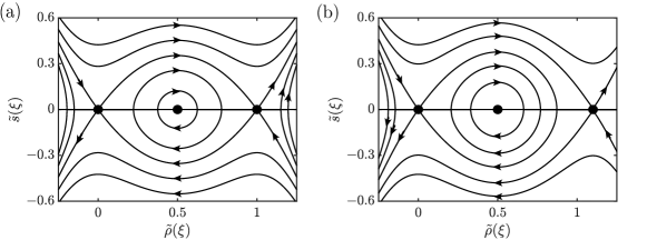
Figure 12: The left panel is a plot of the phase plane of the system (5.6) when $\epsilon=0$. The right panel when $\epsilon=0.1$.

All three of the fixed points persist for $0<\epsilon\ll 1.$ The fixed points $(\tilde{\rho}_{1}^{*},\tilde{s}_{1}^{*})$ and $(\tilde{\rho}_{2}^{*},\tilde{s}_{2}^{*})$ are invariant, whilst $(\tilde{\rho}_{3}^{*},\tilde{s}_{3}^{*})$ translates rightwards in phase space. Furthermore, when $\epsilon>0$ the system (5.6) no longer possesses heteroclinic orbits. Instead, the saddle point $(\tilde{\rho}_{1}^{*},\tilde{s}_{1}^{*})$ has a homoclinic orbit which is order $\sqrt{\epsilon}$ close to the heteroclinic connections, see Figure 12. Using results in [13], the homoclinic orbit is explicitly described by

$$(\tilde{\rho}_{\epsilon}(\xi),\tilde{s}_{\epsilon}(\xi))=\left(\frac{a}{1+b\cosh(c\xi)},-\frac{abc\sinh(c\xi)}{(1+b\cosh(c\xi))^{2}}\right)$$ (5.9)

where

$$a=\frac{12(1+\epsilon)}{12+8\epsilon},\quad b=\sqrt{1-144\frac{1+\epsilon}{(12+8\epsilon)^{2}}}\quad\text{and}\quad c=\sqrt{2(1+\epsilon)}.$$

The pulse $\tilde{\rho}_{\epsilon}(\xi)$ is centred at $\xi=0$ in physical space. Setting $\xi=0$ in (5.9) one obtains the maximum height of the pulse. As $\epsilon\to 0,$ the maximum height of the pulse tends to one and the pulse widens. Note that substituting $\epsilon=0$ into (5.9) yields the saddle point $(\tilde{\rho}_{3}^{*},\tilde{s}_{3}^{*})$. Finally we obtain a relationship between the perturbation parameter $\epsilon$ and the width of the pulse. Defining $L>0$ to be such that $\tilde{\rho}_{\epsilon}(\pm L)=1/2$, one obtains

$$L=\frac{1}{c}\operatorname{arccosh}\left(\frac{3+4\epsilon}{b(3+2\epsilon)}\right)=\frac{1}{\sqrt{2}}\log\bigg{(}\frac{2\sqrt{3}}{\sqrt{\epsilon}}\bigg{)}(1+\mathcal{O}(\epsilon)).$$

This is an invertible relation between $L$ and the small parameter $\epsilon$ and leads to a function $\epsilon(L)$ satisfying $\epsilon(L)=12\exp(-2\sqrt{2}L)(1+\mathcal{O}(L\exp(-2\sqrt{2}L)))$.

Returning to the original spatial variable $x$, the above results to give the following Lemma.

Lemma 8

Consider $0<\epsilon,\delta\ll 1.$ Then the ODE (5.5) with boundary conditions $\rho(\pm\infty)=0$ has solution

$$\rho_{\delta}(x;\epsilon)=\frac{12(1+\epsilon)}{(12+8\epsilon)\left(1+\sqrt{1-144\frac{(1+\epsilon)}{(12+8\epsilon)^{2}}}\cosh\big{(}\sqrt{2(1+\epsilon)}x/\delta\big{)}\right)}.$$ (5.10)

Define $\Delta>0$ to be such that $\rho_{\delta}(\pm\Delta;\epsilon)=1/2$, then

$$\frac{\Delta}{\delta}=\frac{1}{c}\operatorname{arccosh}\left(\frac{3+4\epsilon}{b(3+2\epsilon)}\right)=\frac{1}{\sqrt{2}}\log\bigg{(}\frac{2\sqrt{3}}{\sqrt{\epsilon}}\bigg{)}(1+\mathcal{O}(\epsilon)).$$

This is an invertible relation between $\Delta/\delta$ and $\epsilon$ and leads to a function $\epsilon(\Delta/\delta)$ satisfying

$$\epsilon(\Delta/\delta)=12\exp\left(\frac{-2\sqrt{2}\Delta}{\delta}\right)\left(1+\mathcal{O}\left(\frac{\Delta}{\delta}\exp\left(\frac{-2\sqrt{2}\Delta}{\delta}\right)\right)\right).$$ (5.11)

Furthermore, the pulse $\rho_{\delta}$ approximates $\rho_{0}$. To be specific, for fixed $\Delta>0$ in the three regions

$$R^{-}:=(-\infty,-\Delta-\delta^{a}],\quad R^{0}:=[-\Delta+\delta^{a},\Delta-\delta^{a}],R^{+}:=[\Delta+\delta^{a-1},\infty),$$

the pulses satisfy $|(\rho_{\delta}(x;\epsilon(\Delta/\delta))-\rho_{0}(x;\Delta),s_{\delta}(x;\epsilon(\Delta/\delta)))|=\mathcal{O}\left(\exp\left(-\sqrt{2}\delta^{a-1}\right)\right)$ for any $0<a<1.$

5.2 The extended slow-fast system

Here we extend the inhomogeneous system (5.1) with the equation (5.5) to describe a smooth steep spatial inhomogeneity $\rho$. To be specific, we consider the following system

$$\begin{split}u_{xx}&=(1-d\rho)\sin u\cos v,\\ v_{xx}&=(1-d\rho)\sin v\cos u-\alpha\sin 2v,\\ \delta^{2}\rho_{xx}&=4\rho^{3}-(6+4\epsilon(\Delta/\delta))\rho^{2}+2(1+\epsilon(\Delta/\delta))\rho,\end{split}$$ (5.12)

where $u$, $v$, and $\rho$ are the dependent variables whilst $d$, $\Delta$, and $\alpha$ are constants. The perturbation parameter $0<\delta\ll 1$ corresponds to the steepness of the smooth spatial inhomogeneity. Furthermore, $0<\epsilon(\Delta/\delta)\ll 1$ is given by the condition $\rho(\pm\Delta;\epsilon)=1/2$ and satisfies (5.11). Thus $\epsilon(\Delta/\delta)$ is determined by both the length and steepness of the spatial inhomogeneity. For fixed $\Delta>0,$ $\epsilon(\Delta/\delta)\to 0$ as $\delta\to 0$ and $0<\epsilon\ll\delta\ll 1$.

Notice that the third equation of (5.12) is independent of the first two. On the other hand, the first two equations in (5.12) are coupled to each other and the last equation in the system. We can rewrite (5.12) as the following six dimensional first order dynamical system,

$$\begin{split}u_{x}&=p,\\ p_{x}&=(1-d\rho)\sin u\cos v,\\ v_{x}&=q,\\ q_{x}&=(1-d\rho)\sin v\cos u-\alpha\sin 2v,\\ \delta\rho_{x}&=s,\\ \delta s_{x}&=4\rho^{3}-(6+4\epsilon(\Delta/\delta))\rho^{2}+2(1+\epsilon(\Delta/\delta))\rho.\end{split}$$ (5.13)

We call this the ‘slow’ system. This system has saddle points at

$$\mathcal{B}_{-\infty}=(0,0,0,0,0,0)\quad\text{and}\quad\mathcal{B}_{+\infty}=(2\pi,0,0,0,0,0).$$

We are interested in solutions of the ‘slow’ system (5.13) with the boundary conditions

$$\lim_{x\to-\infty}(u,p,v,q,\rho,s)(x)=\mathcal{B}_{-\infty}\quad\text{and}\quad\lim_{x\to+\infty}(u,p,v,q,\rho,s)(x)=\mathcal{B}_{+\infty}.$$

Upon making the change of variable $x=\delta\xi$ we obtain the ‘fast’ system,

$$\begin{split}\tilde{u}_{\xi}&=\delta\tilde{p},\\ \tilde{p}_{\xi}&=\delta(1-d\tilde{\rho})\sin\tilde{u}\cos\tilde{v},\\ \tilde{v}_{\xi}&=\delta\tilde{q},\\ \tilde{q}_{\xi}&=\delta((1-d\tilde{\rho})\sin\tilde{v}\cos\tilde{u}-\alpha\sin 2\tilde{v}),\\ \tilde{\rho}_{\xi}&=\tilde{s},\\ \tilde{s}_{\xi}&=4\tilde{\rho}^{3}-(6+4\epsilon(\Delta/\delta))\tilde{\rho}^{2}+2(1+\epsilon(\Delta/\delta))\tilde{\rho}.\end{split}$$ (5.14)

Note that the last two equations in the ‘fast’ system (5.14) are exactly the system (5.6).

The slow and fast systems (5.13) and (5.14) are equivalent when $\delta\neq 0$. However they are not equivalent in the limit $\delta\to 0$. Furthermore, the system (5.13) is singularly perturbed in the limit $\delta\to 0$. We first study both systems when $\delta\to 0$. Then we use regular and singular perturbation theory to analyse the systems when $0<\delta\ll 1$.

5.3 Dynamics of the extended system in the limit ${\bm{\delta\to 0}}$

5.3.1 Fast dynamics

When $\delta\to 0,$ the ‘fast’ system (5.14) reduces to the planar system (5.7) and $(\tilde{u},\tilde{p},\tilde{v},\tilde{q})$ staying constant. We call this the ‘fast’ reduced system (FRS). Recall that (5.7) has saddle points $(\tilde{\rho},\tilde{s})=(0,0)$ and $(\tilde{\rho},\tilde{s})=(1,0).$ Thus, we can define the following 4-dimensional normally hyperbolic invariant slow manifolds

$$\begin{split}\mathcal{M}_{0}^{l}=\{(\tilde{u},\tilde{p},\tilde{v},\tilde{q},\tilde{\rho},\tilde{s})=(\tilde{u},\tilde{p},\tilde{v},\tilde{q},0,0)\hskip 6.0pt|\hskip 6.0pt(\tilde{u},\tilde{p},\tilde{v},\tilde{q})\in\mathbb{R}^{4}\},\\ \mathcal{M}_{0}^{r}=\{(\tilde{u},\tilde{p},\tilde{v},\tilde{q},\tilde{\rho},\tilde{s})=(\tilde{u},\tilde{p},\tilde{v},\tilde{q},1,0)\hskip 6.0pt|\hskip 6.0pt(\tilde{u},\tilde{p},\tilde{v},\tilde{q})\in\mathbb{R}^{4}\}.\end{split}$$

The manifolds $\mathcal{M}_{0}^{l/r}$ have 5-dimensional stable and unstable manifolds $\mathcal{W}^{s/u}(\mathcal{M}_{0}^{l/r})$. We are interested in the connections between the manifolds $\mathcal{W}^{s/u}(\mathcal{M}_{0}^{l})$ and $\mathcal{W}^{s/u}(\mathcal{M}_{0}^{r})$ which correspond to the one dimensional heteroclinic connections (5.8) of the saddle points $(\tilde{\rho},\tilde{s})=(0,0)$ and $(\tilde{\rho},\tilde{s})=(1,0)$ in the 4-parameter family $(\tilde{u},\tilde{p},\tilde{v},\tilde{q})\in\mathbb{R}^{4}$.

5.3.2 Slow dynamics

On the other hand taking $\delta\to 0$ in the ‘slow’ system (5.13) yields the following differential-algebraic system,

$$\begin{split}u_{x}&=p,\\ p_{x}&=(1-d\rho)\sin u\cos v,\\ v_{x}&=q,\\ q_{x}&=(1-d\rho)\sin v\cos u-\alpha\sin 2v,\\ 0&=s,\\ 0&=4\rho^{3}-6\rho^{2}+2\rho.\end{split}$$ (5.15)

We call this the ‘slow’ reduced system (SRS). Solving the last two algebraic equations in this system yields the solution set $(\rho,s)=\{(0,0),(1/2,0),(1,0)\}$. These are exactly the fixed points of (5.7). The point $(\rho,s)=(0,0)$ corresponds to the slow manifold $\mathcal{M}_{0}^{l}$ and the slow dynamics on this manifold is

$$u_{x} =p,\quad p_{x}=\sin u\cos v;$$

$$v_{x} =q,\quad q_{x}=\sin v\cos u-\alpha\sin 2v.$$

Similarly the point $(\rho,s)=(1,0)$ corresponds to $\mathcal{M}_{0}^{r}$ and the slow dynamics on this manifold is

$$u_{x} =p,\quad p_{x}=(1-d)\sin u\cos v;$$

$$v_{x} =q,\quad q_{x}=(1-d)\sin v\cos u-\alpha\sin 2v.$$

The dynamics of the system (5.1) with the piecewise constant spatial inhomogeneity $\rho(x;\Delta)=\rho_{0}(x;\Delta)$ can be described as the slow dynamics on $\mathcal{M}_{0}^{l}$ for $|x|>\Delta$ and on $\mathcal{M}_{0}^{r}$ for $|x|<\Delta$ with matching conditions at $|x|=\Delta$. The slow dynamics on the four dimensional manifold $\mathcal{M}_{0}^{l}$ have a fixed point $B_{-\infty}$ at $(u,p,v,q)=(0,0,0,0)$ and $B_{+\infty}$ at $(u,p,v,q)=(2\pi,0,0,0)$. These fixed points are saddles with two dimensional stable and two dimensional unstable manifolds. Denote the unstable manifold to $B_{-\infty}$ by $\mathcal{W}_{0,\text{slow}}^{u}(B_{-\infty})$ and the stable manifold to $B_{+\infty}$ by $\mathcal{W}_{0,\text{slow}}^{s}(B_{+\infty})$.

If $\bm{F_{0}}=(u_{0}(x),v_{0}(x))$ is a stationary solution to (5.1), with piecewise constant spatial inhomogeneity given by $\rho_{0}(x;\Delta)$ and satisfies the boundary conditions (5.2), then $(u_{0},p_{0},v_{0},q_{0})=(u_{0},\partial_{x}u_{0},v_{0},\partial_{x}v_{0})$ lies on the unstable manifold $\mathcal{W}_{0,\text{slow}}^{u}(B_{-\infty})$ for $x<-\Delta$ and on the stable manifold $\mathcal{W}_{0,\text{slow}}^{s}(B_{+\infty})$ for $x>\Delta$. Then the existence of a unique transverse solution $\bm{F_{0}}$ is equivalent to continuing the solutions on the two dimensional unstable manifold $\mathcal{W}_{0,\text{slow}}^{u}(B_{-\infty})$ at $x=-\Delta$ with the flow of the system on $\mathcal{M}_{0}^{r}$ up to $x=\Delta$ and matching one of them to a unique solution on the stable manifold $\mathcal{W}_{0,\text{slow}}^{s}(B_{+\infty})$. Hence the transversality of $\bm{F_{0}}$ refers to a transverse intersection of the continuation of the two-dimensional unstable manifold with the two-dimensional stable manifold in the four dimensional $(u,p,v,q)$ space. Since the system is Hamiltonian, the transverse intersection is one dimensional, despite the fact that a dimension count suggests that the intersection is zero dimensional.

5.3.3 Combining the geometry of the slow and fast dynamics

Both the two dimensional stable and unstable manifolds $\mathcal{W}_{0,\text{slow}}^{s}(B_{+\infty})$ and $\mathcal{W}_{0,\text{slow}}^{u}(B_{-\infty})$ are subsets of the four dimensional slow manifold $\mathcal{M}_{0}^{l}$. Recall that $\bm{F_{0}}(x)$ lies on $\mathcal{W}_{0,\text{slow}}^{u}(B_{-\infty})$ for $x<-\Delta$ and on $\mathcal{W}_{0,\text{slow}}^{s}(B_{+\infty})$ for $x>\Delta$. Define $\bm{F_{0}}(\pm\Delta)=(u_{0}^{\pm},p_{0}^{\pm},v_{0}^{\pm},q_{0}^{\pm})\in\mathbb{R}^{4}$ where by assumption $p_{0}^{\pm}=\partial_{x}u_{0}(\pm\Delta)\neq 0$ and $q_{0}^{\pm}=\partial_{x}v_{0}(\pm\Delta)\neq 0$. This ensures that $\mathcal{W}_{0,\text{slow}}^{s}(B_{+\infty})$ and $\mathcal{W}_{0,\text{slow}}^{u}(B_{-\infty})$ can be written as graphs over $u$ and $v$. Hence nearby $\bm{F_{0}}(\pm\Delta)$, the manifolds $\mathcal{W}_{0,\text{slow}}^{s}(B_{+\infty})$ and $\mathcal{W}_{0,\text{slow}}^{u}(B_{-\infty})$ can be characterised by their $(u,v)$ values at $x=\pm\Delta$ and give two dimensional sub-manifolds in $\mathcal{M}_{0}^{l}:$

$$\overline{\mathcal{W}}_{0,\text{slow}}^{u} := \{(u,p_{0}^{u}(u,v),v,q_{0}^{u}(u,v))\mid(u,v)\mbox{ near }(u_{0}^{-},v_{0}^{-})\},$$

$$\overline{\mathcal{W}}_{0,\text{slow}}^{s} := \{(u,p_{0}^{s}(u,v),v,q_{0}^{s}(u,v))\mid(u,v)\mbox{ near }(u_{0}^{+},v_{0}^{+})\}.$$

Flowing the unstable sub-manifold $\overline{\mathcal{W}}_{0,\text{slow}}^{u}$ forward with the flow of the slow system on $\mathcal{M}_{0}^{r}$ for a $\Delta$ length gives a three dimensional manifold containing $(u_{0},p_{0},v_{0},q_{0})([-\Delta,0])$. Similarly, flowing the stable sub-manifold $\overline{\mathcal{W}}_{0,\text{slow}}^{s}$ backwards with the flow of the slow system on $\mathcal{M}_{0}^{r}$ for length $\Delta$ gives a three dimensional manifold containing $(u_{0},p_{0},v_{0},q_{0})([0,\Delta])$. We will denote these manifolds as

$$\overline{\mathcal{W}}_{0,\text{slow}}^{u,r} = \{\Phi_{x,-\Delta}^{0,r,\text{s}low}(u,p,v,q)\mid(u,p,v,q)\in\overline{\mathcal{W}}_{0,\text{slow}}^{u},\,x\in[-\Delta,0]\},$$

$$\overline{\mathcal{W}}_{0,\text{slow}}^{s,r} = \{\Phi_{x,\Delta}^{0,r,\text{s}low}(u,p,v,q)\mid(u,p,v,q)\in\overline{\mathcal{W}}_{0,\text{slow}}^{s},\,x\in[0,\Delta]\},$$

where $\Phi_{x,x_{0}}^{0,r,\text{s}low}$ denotes the flow of the slow system on the right slow manifold $\mathcal{M}_{0}^{r}$. The transversality assumption on $\bm{F_{0}}$ implies that the boundaries of these two manifolds at $x=0$ intersect transversely.

On the other hand flowing the unstable sub-manifold $\overline{\mathcal{W}}_{0,\text{slow}}^{u}$ backwards with the flow of the slow system on $\mathcal{M}_{0}^{l}$ gives a three dimensional manifold containing $(u_{0},p_{0},v_{0},q_{0})((-\infty,-\Delta])$. Similarly, flowing the stable sub-manifold $\overline{\mathcal{W}}_{0,\text{slow}}^{s}$ forward with the flow of the slow system on $\mathcal{M}_{0}^{l}$ gives a three dimensional manifold containing $(u_{0},p_{0},v_{0},q_{0})([\Delta,+\infty))$. We will denote these manifolds as

$$\overline{\mathcal{W}}_{0,\text{slow}}^{u,l} = \{\Phi^{0,l,slow}_{x,-\Delta}(u,p,v,q)\mid(u,p,v,q)\in\overline{\mathcal{W}}_{0,\text{slow}}^{u},\,x\in(-\infty,-\Delta]\},$$

$$\overline{\mathcal{W}}_{0,\text{slow}}^{s,l} = \{\Phi^{0,l,slow}_{x,\Delta}(u,p,v,q)\mid(u,p,v,q)\in\overline{\mathcal{W}}_{0,\text{slow}}^{s},\,x\in[\Delta,\infty)\}$$

where $\Phi_{x,x_{0}}^{0,l,\text{s}low}$ denotes the flow of the slow system on the left slow manifold $\mathcal{M}_{0}^{l}$.

Extending these sets with either the unstable respectively stable manifolds of the fast dynamics or the fixed points gives the following three dimensional manifolds in $\mathbb{R}^{6}$

$${\mathcal{S}}_{0}^{u,l} = \{(u,p,v,q,0,0)\mid(u,p,v,q)\in\overline{\mathcal{W}}_{0,\text{slow}}^{u,l}\};$$

$${\mathcal{S}}_{0}^{s,l} = \{(u,p,v,q,0,0)\mid(u,p,v,q)\in\overline{\mathcal{W}}_{0,\text{slow}}^{s,l}\};$$

$$\mathcal{S}_{0}^{u} = \{(u,p,v,q,\tilde{\rho}_{0}^{+}(\xi),\tilde{s}_{0}^{+}(\xi))\mid(u,p,v,q)\in\overline{\mathcal{W}}_{0,\text{slow}}^{u},\,\xi\in\mathbb{R}\};$$

$$\mathcal{S}_{0}^{s} = \{(u,p,v,q,\tilde{\rho}_{0}^{-}(\xi),\tilde{s}_{0}^{-}(\xi))\mid(u,p,v,q)\in\overline{\mathcal{W}}_{0,\text{slow}}^{s},\,\xi\in\mathbb{R}\};$$

$${\mathcal{S}}_{0}^{u,r} = \{(u,p,v,q,1,0)\mid(u,p,v,q)\in\overline{\mathcal{W}}_{0,\text{slow}}^{u,r}\};$$

$${\mathcal{S}}_{0}^{s,r} = \{(u,p,v,q,1,0)\mid(u,p,v,q)\in\overline{\mathcal{W}}_{0,\text{slow}}^{s,r}\}.$$

Here $(\tilde{\rho}_{0}^{\pm},\tilde{s}_{0}^{\pm})(\xi)$ are the heteroclinic connections (5.8) between saddle points $(0,0)$ to $(1,0)$ in the FRS. Note $\mathcal{S}_{0}^{u}$ is a three dimensional submanifold of the five dimensional unstable manifold of $\mathcal{M}_{0}^{l}$ and $\mathcal{S}_{0}^{s}$ is a three dimensional submanifold of the five dimensional stable manifold of $\mathcal{M}_{0}^{l}$. To capture a full neighbourhood of the solution associated with $\bm{F_{0}}(x)$, we combine these manifolds as follows (see Figure 13):

$$\mathcal{T}_{0}^{u} = \mathcal{S}_{0}^{u,l}\cup\mathcal{S}_{0}^{u}\cup\mathcal{S}_{0}^{u,r};$$

$$\mathcal{T}_{0}^{s} = \mathcal{S}_{0}^{s,l}\cup\mathcal{S}_{0}^{s}\cup\mathcal{S}_{0}^{s,r}.$$

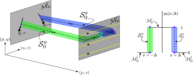
Figure 13: The figure depicts a sketch of the manifolds of the system (5.13) in the limit $\delta\to 0.$ The left grey manifold represents $\mathcal{M}_{0}^{l}$ and the black curves on it represent the unstable and stable manifolds of $\mathcal{B}_{\pm\infty}$ on which $\bm{F_{0}}$ lies for $|x|>\Delta$. The right grey manifold represents $\mathcal{M}_{0}^{r}$ and the yellow curves depict the flow on this manifold with the black curve corresponding to $\bm{F_{0}}$ for $|x|<\Delta$. The purple dots correspond to $(u_{0}^{\pm},p_{0}^{\pm},v_{0}^{\pm},q_{0}^{\pm})$. The green manifold in $\mathcal{M}_{0}^{r}$ represents $\mathcal{S}_{0}^{u,r}$ and the blue manifold in $\mathcal{M}_{0}^{r}$ represents $\mathcal{S}_{0}^{s,r}$. The light blue curves are the edges of $\mathcal{S}_{0}^{u,r}$ and $\mathcal{S}_{0}^{s,r}$ when $x=0$. This illustrates the transverse intersection of these edges.

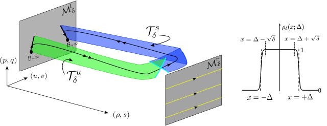
Figure 14: The figure depicts a sketch of the manifolds of the system (5.13) when $0<\delta\ll 1$. The left grey manifold is the persisting manifold $\mathcal{M}_{\delta}^{l}=\mathcal{M}_{0}^{l}$ and the right grey manifold represents $\mathcal{M}_{\delta}^{r}.$ The bold black curves on $\mathcal{M}_{\delta}^{l}$ depict the relevant unstable and stable manifolds of $\mathcal{B}_{\pm\infty}$. The yellow curves on $\mathcal{M}_{\delta}^{r}$ represent the flow on this manifold. The front green manifold is the part of the unstable manifold of the origin, $\mathcal{T}_{\delta}^{u}$, while the back blue manifold is the part of the stable manifold of $(2\pi,0,0,0,0,0)$, $\mathcal{T}_{\delta}^{s}$. The black curve is the persisting solution $\bm{F_{\delta}}$. The double arrows represent fast transition whilst the single represent slow dynamics. To the right is a sketch of $\rho_{\delta}(x;\Delta)$ and the regions we split $\mathcal{T}_{\delta}^{u/s}$ into.

5.4 Dynamics of the extended system when $\bm{0<\delta\ll 1}$

When $0<\delta\ll 1$, the dynamics of the fast variables $(\rho,s)$ remain uncoupled from the slow $(u,p,v,q)$ variables. This two dimensional fast sub-system is given by (5.6) with $\epsilon(\Delta/\delta)$ approximated by (5.11). Its limit for $\delta\to 0$ (i.e. also $\epsilon\to 0$) is (5.7). The fixed points of (5.7) persist for $\delta>0$, see section 5.1. However, the heteroclinic connections in (5.7) do not persist. Instead a homoclinic connection to the origin is created. This connection is denoted by $(\rho_{\delta},s_{\delta})$ and is explicitly described in the slow variables by (5.10). Recall that $\epsilon(\Delta/\delta)$ is such that $\rho_{\delta}(\pm\Delta)=1/2$.

The persistence of the fixed points in the two dimensional fast sub-system implies that the full system (5.14) has $4$-dimensional normally hyperbolic invariant slow manifolds, explicitly given by

$$\mathcal{M}_{\delta}^{l}=\{(\tilde{u},\tilde{p},\tilde{v},\tilde{q},0,0)\},\quad\mathcal{M}_{\delta}^{r}=\{(\tilde{u},\tilde{p},\tilde{v},\tilde{q},1+\epsilon(\Delta/\delta),0)\}.$$

Notice that $\mathcal{M}_{\delta}^{l}=\mathcal{M}_{0}^{l}$ and in the slow variable the flow on $\mathcal{M}_{\delta}^{l}$ is also governed by

$$u_{x} =p,\quad p_{x}=\sin u\cos v;$$

$$v_{x} =q,\quad q_{x}=\sin v\cos u-\alpha\sin 2v.$$

Whilst on $\mathcal{M}_{\delta}^{r}$ it is governed by

$$u_{x} =p,\quad p_{x}=(1-d(1+\epsilon(\Delta/\delta)))\sin u\cos v;$$

$$v_{x} =q,\quad q_{x}=(1-d(1+\epsilon(\Delta/\delta)))\sin v\cos u-\alpha\sin 2v.$$

Note that the flow on $\mathcal{M}_{0}^{r}$ is given by the above with $\epsilon=0$.

Recall that $\mathcal{B}_{-\infty}=(0,0,0,0,0,0)$ and $\mathcal{B}_{+\infty}=(2\pi,0,0,0,0,0)$ are saddle points. On the three dimensional stable manifold $\mathcal{W}_{\delta}^{s}(\mathcal{B}_{+\infty})$ we can define the solution

$$\mathbf{u}_{\delta}^{s}(x;u,v):=(u^{s}_{\delta}(x;u,v),p_{\delta}^{s}(x;u,v),v^{s}_{\delta}(x;u,v),q_{\delta}^{s}(x;u,v),\rho_{\delta}(x),s_{\delta}(x))$$

for $(u,v)$ near $(u_{0}^{+},v_{0}^{+})$. Whilst on the three dimensional unstable manifold $\mathcal{W}_{\delta}^{u}(\mathcal{B}_{-\infty})$ we can define the solution

$$\mathbf{u}_{\delta}^{u}(x;u,v):=(u^{u}_{\delta}(x;u,v),p_{\delta}^{u}(x;u,v),v^{u}_{\delta}(x;u,v),q_{\delta}^{u}(x;u,v),\rho_{\delta}(x),s_{\delta}(x))$$

for $(u,v)$ near $(u_{0}^{-},v_{0}^{-})$. Next we form manifolds by flowing $\mathbf{u}_{\delta}^{s}(x;u,v)$ and $\mathbf{u}_{\delta}^{u}(x;u,v)$ forwards respectively backwards:

$$\mathcal{T}_{\delta}^{s} = \{\mathbf{u}^{s}_{\delta}(x;u,v)\mid(u,v)\mbox{ near }(u_{0}^{+},v_{0}^{+}),\,x\in[0,\infty)\};$$

$$\mathcal{T}_{\delta}^{u} = \{\mathbf{u}^{u}_{\delta}(x;u,v)\mid(u,v)\mbox{ near }(u_{0}^{-},v_{0}^{-}),\,x\in(-\infty,0]\}.$$

Hence these manifolds are part of $\mathcal{W}_{\delta}^{s}(\mathcal{B}_{+\infty})$ and $\mathcal{W}_{\delta}^{u}(\mathcal{B}_{-\infty})$ respectively. See Figure 14 for a sketch of the manifolds $\mathcal{T}_{\delta}^{u/s}$.

We want to show that $\mathcal{T}_{\delta}^{u}$ converges to $\mathcal{T}_{0}^{u}$ and $\mathcal{T}_{\delta}^{s}$ to $\mathcal{T}_{0}^{s}$ as $\delta$ goes to 0. Since $\rho_{0}^{\pm}$ are heteroclinic connections and $\rho_{\delta}$ a homoclinic one, the parametrisation of these orbits is different. Consequently, the $\xi$ parametrisation of $\mathcal{T}_{0}^{u/s}$ is different from the $\xi=x/\delta$ parametrisation in $\mathcal{T}_{\delta}^{u/s}$. But this is not important as we want to compare them as manifolds. To show the convergence, we split both manifolds $\mathcal{T}_{\delta}^{u/s}$ in three parts. We have seen in Lemma 8 that

$$|(\rho_{\delta}(x)-1,s_{\delta}(x))|=\mathcal{O}(e^{-\sqrt{2/\delta}})\text{, for }x\in(-\Delta+\sqrt{\delta},\Delta-\sqrt{\delta}).$$

Hence we split the manifold $\mathcal{T}_{\delta}^{u}$ as follows

$$\mathcal{T}_{\delta,\text{I}}^{u} = \{(\mathbf{u}^{u}_{\delta}(x;u,v)\mid(u,v)\mbox{ near }(u_{0}^{-},v_{0}^{-}),\,x\leqslant-\Delta\};$$

$$\mathcal{T}_{\delta,\text{II}}^{u} = \{(\mathbf{u}^{u}_{\delta}(x;u,v)\mid(u,v)\mbox{ near }(u_{0}^{-},v_{0}^{-}),\,-\Delta\leqslant x\leqslant-\Delta+\sqrt{\delta}\};$$

$$\mathcal{T}_{\delta,\text{III}}^{u} = \{(\mathbf{u}^{u}_{\delta}(x;u,v)\mid(u,v)\mbox{ near }(u_{0}^{-},v_{0}^{-}),\,-\Delta+\sqrt{\delta}\leqslant x\leqslant 0\}.$$

Similarly, we split the manifold $\mathcal{T}_{\delta}^{s}$ as follows

$$\mathcal{T}_{\delta,\text{I}}^{s} = \{(\mathbf{u}^{s}_{\delta}(x;u,v)\mid(u,v)\mbox{ near }(u_{0}^{+},v_{0}^{+}),\,x\geqslant\Delta\};$$

$$\mathcal{T}_{\delta,\text{II}}^{s} = \{(\mathbf{u}^{s}_{\delta}(x;u,v)\mid(u,v)\mbox{ near }(u_{0}^{+},v_{0}^{+}),\,\Delta-\sqrt{\delta}\leqslant x\leqslant\Delta\};$$

$$\mathcal{T}_{\delta,\text{III}}^{s} = \{(\mathbf{u}^{s}_{\delta}(x;u,v)\mid(u,v)\mbox{ near }(u_{0}^{+},v_{0}^{+}),\,0\leqslant x\leqslant\Delta-\sqrt{\delta}\}.$$

We have sketched all relevant manifolds in Figure 14. Next we will prove the convergence.

• Fenichel’s second persistence theorem states that the stable and unstable manifolds $W^{s/u}(\mathcal{M}_{\delta}^{l})$ lie locally within $\mathcal{O}(\delta)$ of $W^{s/u}(\mathcal{M}_{0}^{l})$ and are invariant under the dynamics of the full fast system (5.14); see [8, 15]. The manifold $\mathcal{T}_{\delta,\text{I}}^{s}$ is a subset of $\mathcal{W}_{\delta,slow}^{s}(\mathcal{B}_{+\infty})\subset W^{s}(\mathcal{M}_{\delta}^{l})$ and $\mathcal{T}_{\delta,\text{I}}^{u}$ is a subset of $\mathcal{W}_{\delta,slow}^{u}(\mathcal{B}_{-\infty})\subset W^{u}(\mathcal{M}_{\delta}^{l})$ for $\delta>0$. This implies that the manifolds $\mathcal{T}_{\delta,\text{I}}^{u/s}$ are order $\delta$ close to $\mathcal{T}_{0}^{u/s}$ for $\rho\in\left[0,1/2\right]$, i.e. $|x|\geqslant\Delta$ .

• For $-\Delta\leq x\leq-\Delta+\sqrt{\delta}$, the slow variables can change at most order $\sqrt{\delta}$. Furthermore, the set $\{(\rho_{\delta}(x),s_{\delta}(x))\mid-\Delta\leqslant x\leqslant-\Delta+\sqrt{\delta}\}$ is order $\sqrt{\delta}$ close to $\{(\rho_{0}^{+}(\xi),s_{0}^{+}(\xi))\mid\xi\in[0,\infty)\}.$ Hence, we see that the manifolds $\mathcal{T}_{\delta,\text{II}}^{u}$ are order $\sqrt{\delta}$ close to $\mathcal{T}_{0}^{u}$. A similar argument gives that the manifolds $\mathcal{T}_{\delta,\text{II}}^{s}$ are order $\sqrt{\delta}$ close to $\mathcal{T}_{0}^{s}$.

• The previous observation also implies that the set $\{\mathbf{u}^{u}_{\delta}(-\Delta+\sqrt{\delta};u,v)\mid(u,v)\mbox{ near }(u_{0}^{-},v_{0}^{-})\}$ is order $\sqrt{\delta}$ close to the intersection $\mathcal{S}_{0}^{u}\cap\mathcal{S}_{0}^{u,r}\subset\mathcal{T}_{0}^{u}$. And the set $\{\mathbf{u}_{\delta}^{s}(\Delta-\sqrt{\delta};u,v)\mid(u,v)\mbox{ near }(u_{0}^{+},v_{0}^{+})\}$ is order $\sqrt{\delta}$ close to the intersection $\mathcal{S}_{0}^{s}\cap\mathcal{S}_{0}^{s,r}\subset\mathcal{T}_{0}^{s}$. For $x\in[-\Delta+\sqrt{\delta},\Delta-\sqrt{\delta}]$, $(\rho_{\delta}(x),s_{\delta}(x))$ is at least order $\exp(-\sqrt{2/\delta})$ close to $(1,0)$ (see Lemma 8), so on this finite spatial interval, the flow of the perturbed system is order $\exp(-\sqrt{2/\delta})$ close to the flow on $\mathcal{M}_{0}^{r}$. Hence the manifolds $\mathcal{T}_{\delta,\text{III}}^{u/s}$ are order $\sqrt{\delta}$ close to $\mathcal{T}_{0}^{u/s}$.

So we can conclude that $\mathcal{T}_{\delta}^{u/s}$ are order $\sqrt{\delta}$ close to $\mathcal{T}_{0}^{u/s}$ and hence $\mathcal{T}_{\delta}^{u/s}$ converges to $\mathcal{T}_{0}^{u/s}$ when $\delta$ goes to 0. Since $\mathcal{T}_{0}^{u}|_{x=0}$ and $\mathcal{T}_{0}^{s}|_{x=0}$ intersect transversely, $\mathcal{T}_{\delta}^{u}|_{x=0}$ and $\mathcal{T}_{\delta}^{s}|_{x=0}$ will intersect transversely. Thus we can conclude that the heteroclinic connection $\bm{F_{0}}$ persists for $\delta$ small.

6 Discussion

In this paper, we have presented both an analytic and numerical investigation into the existence of stationary fronts in the system (1.1) for $0<\alpha<1/2.$ In Section 2 we showed numerically the existence of a pitchfork bifurcation at some $\alpha\in(0,1/2)$ for all $\Delta>0$ and $d>0$. Then in Section 3, using the piecewise constant approximation $\rho_{0}(x;\Delta)$ given by (1.3), we gave an implicit expression for the bifurcation locus when $d=1$ and approximations for the two cases $\Delta\gg 1$ and $d\gg 1$. In Section 4 we used the implicit expression for $d=1$ from Section 3 to rigorously show existence of a non-zero $v(x)$ component using Lyapunov-Schmidt reduction. Finally, in Section 5 using geometric singular perturbation theory, we showed that if fronts exist for the piecewise constant inhomogeneity $\rho_{0}(x;\Delta)$, they persist for a smooth sharp inhomogeneity $\rho_{\delta}(x;\Delta)$.

The work in this paper provides a broader understanding of what happens to the destabilised front looked at by Braun et al. [2] in the coupled homogeneous system ($d=0$) and how the front can be stabilised in the coupled system using a spatial inhomogeneity. The effect of the spatial inhomogeneity is to stabilise the sine-Gordon front by a small perturbation where the $\psi$-component dips and the $\theta$-component rises around the centre of the transition. Exploring the effects of hat-like (smooth and non-smooth) inhomogeneities on fronts and their interaction is of practical interest, but also yields some interesting mathematical results, especially the rigorous proof of the persistence of fronts when going from non-smooth to smooth inhomogeneities.

Several interesting avenues for future work are possible. Since existence has been established, a natural question would be to consider the stability of the stationary fronts in the system (1.1). Time simulations shown in Figure 2 indicate that the pitchfork bifurcation is supercritical. It should be possible to verify this analytically using Lyapunov-Schmidt reduction, for example as developed for the stability of rolls in the Swift-Hohenberg equation [17, 18]. Computing the stability with respect to forcing or damping terms would also be of practical interest. Alternatively, one could also consider the existence and stability of stationary solutions where both $u$ and $v$ connect to zero as $|x|\rightarrow\infty$ building on the work of of Derks et al. [5].

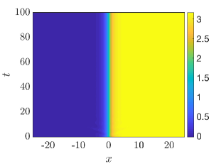
(a) (a)

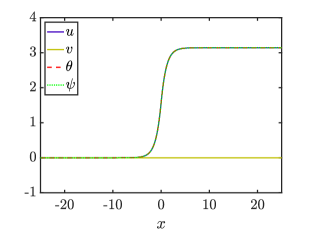
(b) (b)

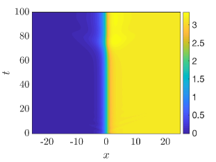
(c) (c)

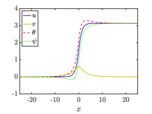
(d) (d)

Figure 15: This figure gives the dynamics of the coupled sine-Gordon system with the step inhomogeneity (6.2) and $d=2$. (a) is a space time plot of $u(x,t=0)=u_{\pi}(x;2)$ with $\alpha=0.2$ and (b) is a plot of the solution profile in (a) at $t=100$. No bifurcation occurs and $u_{\pi}(x)$ is stable. (c) is a space time plot of $u_{\pi}(x)$ with $\alpha=0.45$ and (d) is a plot of the solution profile at $t=100$. The $u_{\pi}(x)$ solution becomes unstable and bifurcates to a new solution. Note we have included a small damping term to suppress the additional radiation in the Hamiltonian system.

Another direction would be to explore the system with other inhomogeneities. The results in this paper can be extended to consider the existence of fronts in the system (1.1) with a smooth “step” inhomogeneity of the form

$$\rho_{\delta}(x)=\frac{\tanh\left(x/\delta\right)+1}{2}.$$ (6.1)

Unlike the hat-like spatial inhomogeneities studied in this paper, the above step has only one jump which is centred at $x=0.$ As $\delta\to 0$ the above converges pointwise to

$$\rho_{0}(x)=\begin{cases}0,&x<0,\\ 1,&x>0.\end{cases}$$ (6.2)

When $d>1$, the system (1.9) with the above piecewise constant inhomogeneity and boundary conditions $(u(-\infty),v(-\infty))=(0,0)$ and $(u(+\infty),v(+\infty))=(\pi,0)$ is known to have solutions $(u_{\pi},0)$ [3] where

$$u_{\pi}(x;d)=\begin{cases}4\arctan(e^{x+x_{1}}),&x<0,\\ 4\arctan(e^{\sqrt{d-1}x+x_{2}})-\pi,&x>0,\end{cases}$$

and $x_{1}(d)$ and $x_{2}(d)$ are matching constants

$$x_{1}(d)=\ln\bigg{(}\tan\bigg{(}\frac{\arccos((2-d)/d)}{4}\bigg{)}\bigg{)}\quad\text{and}\quad x_{2}(d)=\ln\bigg{(}\tan\bigg{(}\frac{\arccos((2-d)/d)+\pi}{4}\bigg{)}\bigg{)}.$$

The bifurcation points of the solution $(u_{\pi}(x),0)$ in the full system (1.9) with spatial inhomogeneity (6.2) are given exactly by the implicit relation (3.5) in Section 3. Time simulations shown in Figure 15 suggest the existence of a bifurcation whereby the $v(x)$ component becomes non-zero, similar to the one studied in this paper. With the explicit front solutions above, one can employ Lyapunov-Schmidt reduction to show the existence of a pitchfork bifurcation and the procedure is almost identical to the one completed in Section 4. Finally, it is possible to show persistence of solutions for the smooth sharp inhomogeneity (6.1) following ideas in Section 5. Setting $\epsilon=0$ in (5.5) means the heteroclinic connections in the fast reduced system persist when $0<\delta\ll 1.$ One then can consider the flow along the stable and unstable manifolds on $\mathcal{M}_{\delta}^{l}$ and $\mathcal{M}_{\delta}^{r}$ respectively and apply Fenichel’s theorems to prove persistence.

Another extension is the generalisation of the smoothening results for an arbitrary smooth sharp inhomogeneity. In this paper we restricted ourselves to using the dynamics of (5.5) to describe the spatial inhomogeneity. However, the ideas extend to any Hamiltonian system that has a bifurcation from a heteroclinic to a homoclinic. The work in Section 5 gives a framework to generalise the smoothening result and prove persistence with respect to a general class of perturbations. A further extension would be to generalise the smoothening result to any system of semi-linear wave equations with spatial inhomogeneities.

Acknowledgements The authors would like to thank Arjen Doelman for inspiring discussions on this problem and the referees for their constructive feedback. JB acknowledges the EPSRC whose institutional Doctoral Training Partnership grant (EP/N509772/1) helped fund his PhD.

The authors confirm that data underlying the findings are available without restriction. Details of the data and how to request access are available via the University of Surrey publications repository.

Appendix A Variation of parameters

Here we determine an expression for $V_{21}$ as required in (4.1). Upon substituting $V_{11}=V_{22}=0,$ which were determined at $\mathcal{O}(A),$ into (4.6b) yields

$$(I-Q)\bigg{(}\mathcal{L}_{0}\bm{V_{2}}+\tilde{\alpha}\mathcal{L}_{1}\bm{V_{2}}+(1-\rho)\left(\begin{array}[]{ c }\Psi^{2}\sin(u_{0})/2\\ 0\end{array}\right)\bigg{)}=\mathbf{0}.$$

We are interested in the first component $V_{21},$ of the vector $\bm{V_{2}},$ which by the above is governed by

$$\frac{d^{2}Y}{dx^{2}}-(1-\rho)\cos(u^{*})Y=-\frac{1}{2}(1-\rho)\sin(u_{0})\Psi^{2}.$$

where we have set $Y=V_{21}$ for notational convenience. To solve this second order ODE we are required to use variation of parameters. Since the integral (4.1) is over the interval $[\Delta,\infty)$ it is only necessary to compute $Y(x)$ in the region $x>\Delta.$ Hence we seek to solve,

$$\frac{d^{2}A}{dx^{2}}-\cos(u_{0})A=-\frac{1}{2}\sin(u_{0})\Psi^{2}.$$ (1.1)

where

$$u_{0}=4\arctan(e^{x-x^{*}}),$$

$$\Psi=-R(\tanh(x-x^{*})+\sqrt{1-2\alpha^{*}})\exp(-\sqrt{1-2\alpha^{*}}(x-x^{*})).$$

The second order ODE

$$\frac{d^{2}Y}{dx^{2}}-\cos(u_{0})Y=0$$

has two linearly independent solutions (see e.g. [3]) given by

$$Y_{1}(x)=\operatorname{sech}(x-x^{*})\quad\text{and}\quad Y_{2}(x)=\sinh(x-x^{*})+\frac{x-x^{*}}{\cosh(x-x^{*})}.$$

Using the variation of parameters method one determines

$$Y(x)=\frac{Y_{1}(x)}{4}\int^{x}Y_{2}(\bar{x})\sin(u_{0}(\bar{x}))\Psi^{2}(\bar{x})d\bar{x}\\ -\frac{Y_{2}(x)}{4}\int^{x}Y_{1}(\bar{x})\sin(u_{0}(\bar{x}))\Psi^{2}(\bar{x})d\bar{x}+AY_{1}(x)+BY_{2}(x),$$

where constants $A$ and $B$ are determined. It can be shown from the boundary conditions $Y(+\infty)=Y^{\prime}(+\infty)=0$ that $B=0.$ Finally since $Y(x)$ is an odd function and $Y_{1}(x)$ is even we must have $A=0.$ Hence,

$$V_{21}(x)=\frac{Y_{1}(x)}{4}\int^{x}Y_{2}(\bar{x})\sin(u_{0}(\bar{x}))\Psi^{2}(\bar{x})d\bar{x}\\ -\frac{Y_{2}(x)}{4}\int^{x}Y_{1}(\bar{x})\sin(u_{0}(\bar{x}))\Psi^{2}(\bar{x})d\bar{x}.$$

Appendix B Expressions for the eigenfunction

Here we determine the matching constant $A$ and the rescaling constant $R$ of the eigenfunction (3.15). Matching the eigenfunction (3.15) at $x=-\Delta$ yields

$$A=-\frac{\bigg{(}\sqrt{1+\Lambda}+\sqrt{\frac{2-h}{2}}\bigg{)}\left(\tan\left(\arccos(1-h)/4\right)\right)^{\sqrt{1+\Lambda}}}{\cos\left(\sqrt{-\Lambda}\Delta\right)}.$$

Now we wish to find the rescaling constant such that $\int_{-\infty}^{+\infty}\Psi^{2}=1.$ Since $\Psi$ is an even function,

$$\frac{1}{R^{2}}=A^{2}\bigg{(}\frac{\sin(2\sqrt{-\Lambda}\Delta)}{2\sqrt{-\Lambda}}+\Delta\bigg{)}+2\int_{\Delta}^{\infty}e^{-2\sqrt{1+\Lambda}(x-x^{*})}(\tanh(x-x^{*})+\sqrt{1+\Lambda})^{2}dx.$$

Hence

$$\frac{1}{R^{2}}=A^{2}\bigg{(}\frac{\sin(2\sqrt{2\alpha^{*}}\Delta)}{2\sqrt{2\alpha^{*}}}+\Delta\bigg{)}\\ +2\bigg{[}\frac{(1-2\alpha+(1-\alpha)\sqrt{1-2\alpha})e^{-2\sqrt{1-2\alpha}(x-x^{*})}}{(e^{2(x-x1)}+1)\alpha^{2}(2\alpha-1)}\\ \times(\alpha^{2}e^{2(x+x^{*})}+2(\alpha-1)\sqrt{1-2\alpha}+\alpha^{2}-4\alpha+2)\bigg{]}_{\Delta}^{\infty}.$$

References

[1]
E. Bour.
Théorie de la déformation des surfaces.
J. Ecole Imperiale Polytechnique, 19:1–48, 1862.
[2]
O M Braun, Yu S Kivshar, and A M Kosevich.
Interaction between kinks in coupled chains of adatoms.
Journal of Physics C: Solid State Physics, 21(21):3881, 1988.
[3]
G. Derks, A. Doelman, S. A. van Gils, and H. Susanto.
Stability analysis of -kinks in a 0- Josephson
junction.
SIAM J. Appl. Dyn. Syst., 6(1):99–141, 2007.
[4]
Gianne Derks, Arjen Doelman, Christopher J. K. Knight, and Hadi Susanto.
Pinned fluxons in a Josephson junction with a finite-length
inhomogeneity.
European J. Appl. Math., 23(2):201–244, 2012.
[5]
Gianne Derks and Giuseppe Gaeta.
A minimal model of DNA dynamics in interaction with
RNA-polymerase.
Phys. D, 240(22):1805–1817, 2011.
[6]
E J Doedel, R C Paffenroth, A R Champneys, T F Fairgrieve, Yu A Kuznetsov, B E
Oldeman, and B Sandstede.
Auto07p: Continuation and bifurcation software for ordinary
differential equations.
Technical report, Concordia University, 2007.
[7]
Arjen Doelman, Peter van Heijster, and Tasso J. Kaper.
Pulse dynamics in a three-component system: Existence analysis.
Journal of Dynamics and Differential Equations, 21(1):73–115,
2009.
[8]
Neil Fenichel.
Geometric singular perturbation theory for ordindary differential
equations.
Journal of Differential Equations, 31:53–98, 1979.
[9]
J. Frenkel and T. Kontorova.
On the theory of plastic deformation and twinning.
Izvestiya Akademii Nauk SSSR, Seriya Fizicheskaya, 1:137–149,
1939.
[10]
S. W. Goatham, L. E. Mannering, R. Hann, and S. Krusch.
Dynamics of multi-kinks in the presence of wells and barriers.
Acta Physica Polonica B, 42:2087–2106, 2011.
[11]
Ryan Goh and Arnd Scheel.
Pattern formation in the wake of triggered pushed fronts.
Nonlinearity, 29(8):2196–2237, 2016.
[12]
Martin Golubitsky and David G. Schaeffer.
Singularities and Groups in Bifurcation Theory, volume 1.
Springer, 1985.
[13]
Samir Hamdi, Brian Morse, Bernard Halphen, and William Schiesser.
Analytical solutions of long nonlinear internal waves: Part i.
Natural Hazards, 57(3):597–607, Jun 2011.
[14]
Shigeo Homma and Shozo Takeno.
A coupled base-rotator model for structure and dynamics of dna.
Progress of Theoretical Physics, 72(4):679–693, October 1984.
[15]
Christopher K. R. T. Jones.
Dynamical Systems, volume 1609 of Lecture notes in
Mathematics, chapter Geometric singular perturbation theory, pages 44–118.
Springer, 1995.
[16]
E. Mann.
Systematic perturbation theory for sine-Gordon solitons without use
of inverse scattering methods.
J. Phys. A: Math. Gen., 30:1227–1241, 1997.
[17]
A. Mielke.
A new approach to sideband-instabilities using the principle of
reduced instability.
In Nonlinear dynamics and pattern formation in the natural
environment (Noordwijkerhout, 1994), volume 335 of Pitman Res. Notes
Math. Ser., pages 206–222. Longman, Harlow, 1995.
[18]
Alexander Mielke.
Instability and stability of rolls in the Swift-Hohenberg
equation.
Comm. Math. Phys., 189(3):829–853, 1997.
[19]
Bernard Piette and W J Zakrzewski.
Scattering of sine-gordon kinks on potential wells.
Journal of Physics A: Mathematical and Theoretical,
40:5995–6010, 2007.
[20]
L. V. Yakushevich.
Nonlinear DNA dynamics: a new model.
Phys. Lett. A, 136:413–417, 1989.