Ghost and tachyon free Poincaré gauge theories: A systematic approach

Abstract

A systematic method is presented for determining the conditions on the parameters in the action of a parity-preserving gauge theory of gravity for it to contain no ghost or tachyon particles. The technique naturally accommodates critical cases in which the parameter values lead to additional gauge invariances. The method is implemented as a computer program, and is used here to investigate the particle content of parity-conserving Poincaré gauge theory, which we compare with previous results in the literature. We find 450 critical cases that are free of ghosts and tachyons, and we further identify 10 of these that are also power-counting renormalizable, of which four have only massless tordion propagating particles and the remaining six have only a massive tordion propagating mode.

I Introduction

Following the gauging of the Lorentz group by Utiyama Utiyama (1956), Kibble was the first to gauge the Poincaré group Kibble (1961). In Kibble’s model, the gauge fields of the Poincaré group are $h\indices{{}_{A}^{\mu}}$ and $A\indices{{}^{AB}_{\mu}}$, which correspond to translations and Lorentz transformations, respectively. Such Poincaré gauge theories (PGTs) have a geometric interpretation in terms of a Riemann–Cartan spacetime ($U_{4}$), which differs from the more familiar Riemann spacetime ($V_{4}$) in having nonzero torsion. In this geometric interpretation, the field strengths of the translational and rotational gauge fields are identified as the torsion and curvature, respectively, of the $U_{4}$ spacetime Blagojević (2002).

The action in PGT has the general form

$$S=\int\mathrm{d}^{4}x\;h^{-1}\left[\mathcal{L}_{\rm G}\left(\mathcal{R}\indices{{}^{AB}_{CD}},\mathcal{T}\indices{{}^{A}_{BC}}\right)+\mathcal{L}_{\rm M}\left(\varphi,\mathcal{D}_{A}\varphi\right)\right],$$ (1)

where $h=\mbox{det}(h\indices{{}_{A}^{\mu}})$, $\mathcal{L}_{\rm G}$ is the free gravitational Lagrangian, $\mathcal{L}_{\rm M}$ is the matter Lagrangian, $\mathcal{R}\indices{{}^{AB}_{CD}}\left(h,A,\partial A\right)$ and $\mathcal{T}\indices{{}^{A}_{BC}}(h,\partial h,A)$ are the field strengths corresponding to the Lorentz and translational parts, respectively, of the Poincaré group, $\mathcal{D}_{A}$ is the covariant derivative, and $\varphi$ is the matter field. Here, Greek indices correspond to the coordinate frame, and capital Latin indices to the local Lorentz frame. The field strengths can be expressed as $\mathcal{R}\indices{{}^{AB}_{CD}}=h\indices{{}_{C}^{\mu}}h\indices{{}_{D}^{\nu}}\mathcal{R}\indices{{}^{AB}_{\mu\nu}}$ and $\mathcal{T}\indices{{}^{A}_{BC}}=h\indices{{}_{B}^{\mu}}h\indices{{}_{C}^{\nu}}\mathcal{T}\indices{{}^{A}_{\mu\nu}}$, where

$$\mathcal{R}\indices{{}^{AB}_{\mu\nu}}=2(\partial_{[\mu}A\indices{{}^{AB}_{\nu]}}+A\indices{{}^{A}_{E[\mu}}A\indices{{}^{EB}_{\nu]}}),$$ (2)

$$\mathcal{T}\indices{{}^{A}_{\mu\nu}}=2(\partial_{[\mu}b\indices{{}^{A}_{\nu]}}+A\indices{{}^{A}_{E[\mu}}b\indices{{}^{E}_{\nu]}}),$$ (3)

and $b\indices{{}^{A}_{\mu}}$ is the inverse $h$-field, such that $b\indices{{}^{A}_{\mu}}h\indices{{}_{B}^{\mu}}=\delta^{A}_{B}$ and $b\indices{{}^{A}_{\mu}}h\indices{{}_{A}^{\nu}}=\delta^{\nu}_{\mu}$.

One property that a healthy theory should possess is unitarity. The particle spectrum of a unitary theory should contain no ghosts (particles with negative free field energy) or tachyons (particles with imaginary masses). Several authors have previously arrived at no-ghost-or-tachyon conditions for some subsets of PGT. For parity-conserving PGT (which we term PGT⁺), Neville Neville (1978, 1980) considered $\mathcal{R}+\mathcal{R}^{2}$ actions, and Sezgin and van Nieuwenhuizen Sezgin and van Nieuwenhuizen (1980) examined the most general action with no more than two derivatives, i.e. $\mathcal{R}+\mathcal{R}\text{}\indices{{}^{2}}+\mathcal{T}^{2}$, using a systematic method with spin projection operators Rivers (1964); van Nieuwenhuizen (1973); Neville (1978). Karananas Karananas (2015) and Blagojević and Cvetković Blagojević and Cvetković (2018) studied the most general $\mathcal{R}+\mathcal{R}\text{}\indices{{}^{2}}+\mathcal{T}^{2}$ action for PGT with parity-violating terms.

If the parameters in the action satisfy certain “critical conditions”, however, the theory may possess additional gauge invariances. This increases the difficulty of obtaining the no-ghost condition of the massless sector of a PGT systematically. Therefore, following a brief primer on spin projections operators and notation in Sec. II, we present in Sec. III a systematic approach to investigating all such critical cases and accommodating the associated additional source constraints; the method is implemented in Mathematica using the MathGR Wang package. We apply our method to PGT⁺ in Sec. IV and compare our results with those previously presented in the literature; we also identify special cases that are not only free of ghosts and tachyons, but also power-counting renormalizable. We conclude in Sec. V.

We use the Landau–Lifshitz metric signature $\eta_{AB}=(+,-,-,-)$ throughout this paper.

II Spin projection operators

We begin by briefly reviewing the spin projection operator (SPO) formalism Rivers (1964); Barnes (1965); Aurilia and Umezawa (1969) and establishing our notation. The SPOs may be used to decompose a field in momentum space into parts with definite spin $J$ and parity $P$.

A field $\zeta_{\acute{\alpha}}$, where a Greek index with an acute accent ($\acute{\alpha}$, …) represents the collection of the local Lorentz indices of the field, may be decomposed as

$$\zeta(k)_{\acute{\alpha}} =\sum_{J,P,i}\zeta_{i}(J^{P},k)_{\acute{\alpha}},$$ (4)

$$\zeta_{i}(J^{P},k)_{\acute{\alpha}} \equiv P_{ii}(J^{P},k)\indices{{}_{\acute{\alpha}}^{\acute{\beta}}}\zeta(k)_{{\acute{\beta}}},$$ (5)

where there is no sum on $i$ in (5). There may be more than one component, or none, with spin-parity $J^{P}$. The index $i$ (or, more generally, lowercase Latin letters from the middle of the alphabet) labels these components in the same spin-parity sector and also labels the SPOs. The momentum $k^{A}$ is a timelike vector, but for simplicity we omit the tensor indices of the momentum $k$ and position $x$ when they appear as function arguments. Indeed, for brevity’s sake, we will omit the dependence of fields and SPOs on $k$ or $x$ for the remainder of this section.

There are also off-diagonal SPOs $P_{ij}(J^{P})\indices{{}_{\acute{\alpha}}^{\acute{\beta}}}$, where $i\neq j$, which complete a basis for parity-conserving operators acting on $\zeta_{\acute{\alpha}}$. The SPO basis is Hermitian, complete, orthonormal, and the diagonal elements are positive (or negative) definite. Thus, they satisfy

$$P_{ij}(J^{P})^{{\acute{\alpha}}{\acute{\beta}}}=P^{\ast}_{ji}(J^{P})^{{\acute{\beta}}{\acute{\alpha}}},$$ (6)

$$\sum_{i,J,P}P_{ii}(J^{P})_{{\acute{\alpha}}{\acute{\beta}}}=\mathbb{I}_{{\acute{\alpha}}{\acute{\beta}}},$$ (7)

$$P_{ik}(J^{P})\indices{{}_{\acute{\alpha}}^{\acute{\mu}}}P_{lj}(J^{\prime P^{\prime}})_{\acute{\mu}{\acute{\beta}}}=\delta_{JJ^{\prime}}\delta_{PP^{\prime}}\delta_{kl}P_{ij}(J^{P})_{{\acute{\alpha}}{\acute{\beta}}},$$ (8)

$$[\varphi^{*}_{\acute{\alpha}}P_{ii}(J^{P})^{{\acute{\alpha}}{\acute{\beta}}}\varphi_{\acute{\beta}}]P\geq 0\quad\forall i,\varphi_{\acute{\alpha}},$$ (9)

where $\mathbb{I}_{{\acute{\alpha}}{\acute{\beta}}}$ is the identity operator for the field $\zeta$, and in the final condition $\varphi_{\acute{\beta}}$ is an arbitrary field in the same tensor space as $\zeta$ and $P$ (without indices) is the parity.

Now consider the (usual) case in which the action contains multiple fields $\zeta^{(1)}_{{\acute{\alpha}}_{1}}$, $\zeta^{(2)}_{{\acute{\alpha}}_{2}}$, …, $\zeta^{(f)}_{{\acute{\alpha}}_{f}}$, where the index $a=1,\ldots,f$ labels the fields (generally we will use lowercase Latin letter from the start of the alphabet for this purpose). One can then generalize the SPO $P_{ij}(J^{P})_{{\acute{\alpha}}{\acute{\beta}}}$ in the single-field case to $P_{ij}^{(ab)}(J^{P})_{{\acute{\alpha}}{\acute{\beta}}}$, where the latter now projects the $j$th part with spin-parity $J^{P}$ of the field $\zeta^{(b)}_{\acute{\beta}}$ into the $i$th part with spin-parity $J^{P}$ of the field $\zeta^{(a)}_{\acute{\alpha}}$.

It is clear from the above discussion that the description of SPOs requires the introduction of several sets of indices of different types. In an attempt to ease somewhat this notational burden, we introduce a matrix-vector formalism that removes two of these sets of indices. We begin by defining the generalized field vector

$$\hat{\zeta}\equiv\sum_{a=1}^{n}\zeta^{(a)}_{\acute{\alpha}_{a}}\mathbf{e}_{a},$$ (10)

where $\mathbf{e}_{a}$ is a column vector with $a$th element equal to unity and the remaining elements zero. On the left-hand side (LHS) of (10), we have suppressed the local Lorentz indices, and it should be understood that the $a$th element of $\hat{\zeta}$ consists of the tensor expression $\zeta^{(a)}_{\acute{\alpha}_{a}}$. The contraction of two generalized field vectors $\hat{\zeta}$ and $\hat{\xi}$ is then given by

$$\hat{\zeta}^{\dagger}\cdot\hat{\xi}=\sum_{a=1}^{n}\zeta^{\ast(a)}_{{\acute{\alpha}}_{a}}\xi^{(a){\acute{\alpha}}_{a}},$$ (11)

where we have “overloaded” the dot notation on the LHS to encompass the summations both over the field index $a$ and the collection of local Lorentz indices $\acute{\alpha}$.

Turning to the SPOs, we begin by considering the tensor quantities $P_{ij}^{(ab)}(J^{P})_{{\acute{\alpha}}{\acute{\beta}}}$ as the elements of a block matrix $\mathsf{P}(J^{P})$, for which the indices $(a,b)$ label the $f\times f$ blocks and the indices $(i,j)$ label the individual elements within each block. Note that since not every field has parts belonging to a given spin-parity sector $J^{P}$, some of the blocks will have zero size. We then redefine the indices $(i,j)$ such that $P_{ij}(J^{P})_{{\acute{\alpha}}{\acute{\beta}}}$ denotes simply the tensor expression in the $i$th row and $j$th column of $\mathsf{P}(J^{P})$. Finally, for each such element, we define the $f\times f$ matrix

$$\hat{P}_{ij}(J^{P})\equiv P_{ij}(J^{P})_{{\acute{\alpha}}{\acute{\beta}}}\mathbf{e}_{a}\mathbf{e}^{\dagger}_{b},$$ (12)

where $(a,b)$ denotes the block in $\mathsf{P}(J^{P})$ to which the element belongs. By analogy with (10), we have again suppressed the local Lorentz indices on the LHS of (12) for brevity. The advantage of this notation is that these generalized quantities (denoted by a caret) satisfy relationships of an analogous form to those given in (7)–(9).

The SPO block matrices $\mathsf{P}(J^{P})$ used in this paper for PGT⁺ are listed in Appendix A. One can obtain the operators for other fields by the method described in Aurilia and Umezawa (1969).

III Method

We determine whether a theory contains ghosts or tachyons by adapting the systematic method of spin projection operators used in Sezgin and van Nieuwenhuizen (1980); Karananas (2015). We apply the method to parity-preserving Lagrangians with arbitrary real tensor fields, for which the linearized Lagrangian can be written as

$$\mathcal{L} =\mathcal{L}_{\rm F}+\mathcal{L}_{\rm I},$$

$$=\tfrac{1}{2}\sum_{a,b}\zeta^{(a)}_{{\acute{\alpha}}}(x)\mathcal{O}^{(ab)}(\partial)^{{\acute{\alpha}}{\acute{\beta}}}\zeta^{(b)}_{{\acute{\beta}}}(x)\!-\!\sum_{a}\zeta^{(a)}_{\acute{\alpha}}(x)j^{(a)\acute{\alpha}}(x),$$

$$=\tfrac{1}{2}\hat{\zeta}^{\rm T}(x)\cdot\hat{\mathcal{O}}(\partial)\cdot\hat{\zeta}(x)-\hat{\zeta}^{\rm T}(x)\cdot\hat{j}(x),$$ (13)

where $\zeta^{(a)}_{\acute{\alpha}}(x)$ are the fields, $j^{(a)}_{\acute{\alpha}}(x)$ are the corresponding source currents, and we have defined the generalized operator $\hat{\mathcal{O}}(\partial)\equiv\mathcal{O}^{(ab)}(\partial)^{{\acute{\alpha}}{\acute{\beta}}}\mathbf{e}_{a}\mathbf{e}_{b}^{\dagger}$ (again suppressing local Lorentz indices on the LHS), in which $\mathcal{O}^{(ab)}(\partial)^{{\acute{\alpha}}{\acute{\beta}}}$ is a polynomial in $\partial$ and depends linearly on the coefficients of the terms in the free-field Lagrangian.

By Fourier transformation, the free-field part of the Lagrangian can be written

$$\mathcal{L}_{\rm F}=\tfrac{1}{2}\hat{\zeta}^{\rm T}(-k)\cdot\hat{\mathcal{O}}(k)\cdot\hat{\zeta}(k),$$ (14)

where, without loss of generality, one may take $\hat{\mathcal{O}}(k)$ to be Hermitian. A theory has no tachyon if all particles have real masses, and it contains no ghost particle if the real parts of the residues of the saturated propagator at all poles are non-negative:

$$\mathrm{Re}\,\left[\underset{k^{2}=m^{2}}{\mathrm{Res}}\left(\Pi\right)\right]\geq 0,$$ (15)

where the saturated propagator is the propagator sandwiched between currents

$$\Pi(k)=\hat{j}^{\dagger}(k)\cdot\hat{\mathcal{O}}^{-1}(k)\cdot\hat{j}(k).$$ (16)

To obtain the propagator, one first decomposes $\hat{\mathcal{O}}(k)$ into sectors with definite spin and parity:

$$\hat{\mathcal{O}}(k)=\sum_{J,P}\hat{\mathcal{O}}(J^{P},k)=\sum_{i,j,J,P}a_{ij}(J^{P},k)\hat{P}_{ij}(J^{P},k).$$ (17)

Pre- and post-multiplying (17) by SPOs and using the orthonormality conditions (8), one obtains (omitting the explicit dependence of quantities on $k$ for brevity)

$$\hat{P}_{ii}(J^{P}) \cdot\hat{\mathcal{O}}\cdot\hat{P}_{jj}(J^{P})$$

$$=\sum_{k,l,J^{\prime},P^{\prime}}a_{kl}(J^{\prime P^{\prime}})\hat{P}_{ii}(J^{P})\cdot\hat{P}_{kl}(J^{\prime P^{\prime}})\cdot\hat{P}_{jj}(J^{P})$$

$$=a_{ij}(J^{P})\hat{P}_{ij}(J^{P}),$$ (18)

from which one can read off $a_{ij}(J^{P})$ as the coefficient of $\hat{P}_{ij}(J^{P})$. The quantity $a_{ij}(J^{P})$ may be considered as the $(i,j)$th element of a $s\times s$ matrix $a(J^{P})$, where $s$ is the number of parts of spin-parity $J^{P}$ across all the fields.

The next step is to invert $\hat{\mathcal{O}}(k)$ to obtain the propagator. The orthonormality property of the SPO means that inverting $\hat{\mathcal{O}}(k)$ is equivalent to inverting the matrices $a(J^{P})$. One may, however, find that some of the $a$-matrices are singular, and so cannot be inverted.

If $a(J^{P})$ is singular, then the theory possesses gauge invariances, as follows. If $a(J^{P})$ has dimension $s\times s$ and rank $r$, then it has $(s-r)$ null right eigenvectors $v_{i}^{w,R}(J^{P})$, where $i$ is the vector component index and $w$ is a label enumerating the null eigenvectors (a null eigenvector is an eigenvector that corresponds to a zero eigenvalue). Similarly, the transpose matrix $a^{\rm T}(J^{P})$ has $(s-r)$ null left eigenvectors $v_{i}^{w,L}(J^{P})$. Thus, if the generalized field $\hat{\zeta}$ is subjected to a change of the form

$$\delta\hat{\zeta}^{w}=\sum_{k,J,P}v_{k}^{w,R}(J^{P})\hat{P}_{kj}(J^{P})\cdot\hat{\varphi},$$ (19)

where $\hat{\varphi}$ is some arbitrary generalized field, then the equations of motion $\hat{\mathcal{O}}\cdot\hat{\zeta}=\hat{j}$ remain unchanged.

The null eigenvectors also lead to constraints on the source currents $\hat{j}$. From the equations of motion, one may show that

$$\sum_{l}v_{l}^{w,L}( J^{P})\hat{P}_{kl}(J^{P})\cdot\hat{j}$$

$$=\sum_{l,i,j}v_{l}^{w,L}(J^{P})\hat{P}_{kl}(J^{P})\cdot a_{ij}(J^{P})\hat{P}_{ij}(J^{P})\cdot\hat{\zeta}$$

$$=\sum_{i,j}\left[v_{i}^{w,L}(J^{P})a_{ij}(J^{P})\right]\hat{P}_{kj}(J^{P})\cdot\hat{\zeta}$$

$$=0\qquad\forall k,J^{P},w.$$ (20)

Hence, one can use the $(s-r)$ field transformations in (19) to set the corresponding $(s-r)$ parts $\zeta_{k}(J^{P})_{\acute{\alpha}}$ of the field to zero and hence fix the gauge. This is equivalent to deleting the corresponding $(s-r)$ rows and columns in $a(J^{P})$, and thereby $a(J^{P})$ becomes nonsingular (this is most easily implemented by successively proposing each row/column pair for deletion, and eliminating only those for which the rank of the matrix is unchanged). We denote the $a-$matrices after deleting the rows and columns by $b(J^{P})$ . Note that, if the rank of $a(J^{P})$ is zero, then there is no particle content in this spin-parity sector and we will ignore these spin-parity sectors in the following discussion.

The inverse of $\hat{\mathcal{O}}(J^{P})$ then becomes

$${\hat{\mathcal{O}}^{-1}}(J^{P})=\sum_{i,j}b^{-1}_{ij}(J^{P})\hat{P}_{ij}(J^{P}),$$ (21)

where $b^{-1}_{ij}(J^{P})$ denotes the $(i,j)$th element of the inverse $b$-matrix, and the saturated propagator is thus given by

$$\Pi=\sum_{i,j,J,P}b^{-1}_{ij}(J^{P})\,\hat{j}^{\dagger}\cdot\hat{P}_{ij}(J^{P})\cdot\hat{j}.$$ (22)

The no-ghost condition (15) requires us to locate the poles of the saturated propagator. We first consider those arising from the elements of the inverse $b$-matrices, which can be written as

$$b^{-1}_{ij}(J^{P})=\frac{1}{\mathrm{det}\left[b(J^{P})\right]}C^{\rm T}_{ij}(J^{P}),$$ (23)

where $C_{ij}(J^{P})$ is the cofactor of the element $b_{ij}(J^{P})$. Since $C_{ij}(J^{P})$ is polynomial in $k$, all poles of $b^{-1}_{ij}(J^{P})$ are located at the zeroes of $\mathrm{det}\left[b(J^{P})\right]$. The determinant in each spin-parity sector can be written as

$$\mathrm{det}\left[b(J^{P})\right]=\alpha k^{2q}(k^{2}-m_{1}^{2})(k^{2}-m_{2}^{2})...(k^{2}-m_{r}^{2}),$$ (24)

where $\alpha$ and $m_{1},m_{2},\ldots,m_{q}$ (which we assume are nonzero) are functions of the Lagrangian parameters but independent of $k$, and $q$ and $r$ are non-negative integers. Thus, $b^{-1}_{ij}(J^{P})$ has poles only at $k^{2}=0$ and $k^{2}=m^{2}_{1}$, $k^{2}=m^{2}_{2}$,…, $k^{2}=m^{2}_{r}$.

It is worth noting that the reason why there are no odd-order $k$ terms in the determinant is that only the off-diagonal elements of $b$-matrices contain odd-order $k$ terms. Such an element must belong to a row and column corresponding to one field with odd indices and the other with even indices. The odd-order $k$ is always accompanied by a factor $i$, so such elements are purely imaginary. Since the $b$-matrix is Hermitian, however, its determinant is real. The terms in odd powers of $k$ must cancel because they are imaginary, and so the determinant contains only terms with even powers of $k$.

III.1 Massless sector

The no-ghost condition (15) in the massless sector is that the residue of the saturated propagator (22) at $k^{2}=0$ be non-negative. Besides the poles at $k^{2}=0$ present in $b^{-1}_{ij}(J^{P})$, the SPOs $P_{ij}(J^{P})$ also contain singularities of the form $k^{-2n}$, where $n$ is a positive integer.

Letting $k^{A}=(E,\vec{p})$ and $p\equiv\sqrt{\vec{p}^{2}}$, the particle energy is given by $E=\sqrt{k^{2}+p^{2}}$, and the saturated propagator can be written (most conveniently in a slightly unorthodox form) as a Laurent series in $k^{2}$ in the neighbourhood of $k^{2}=0$

$$\Pi(k^{2},\vec{p})=\sum_{n=-\infty}^{N}\frac{Q_{2n}}{k^{2n}},$$ (25)

where $N$ is an integer and the coefficients $Q_{2n}$ are some functions of the on-shell momentum $\bar{k}^{A}\equiv(p,\vec{p})$ and the on-shell source currents $j^{(a)}_{\acute{\alpha}}(\bar{k})$. If $N$ is zero or negative, then there is no pole at $k^{2}=0$ and there is no propagating massless particle. We will only discuss the $N>0$ cases here. The no-ghost conditions (15) are that the residue of $k^{2}=0$ be non-negative, so $Q_{2}\geq 0$. Furthermore, we require that the saturated propagator has a simple pole in $k^{2}$ at this point, since terms proportional to $k^{-2n}$ with $n>1$ contain ghost states Heisenberg (1957). For example, if the Laurent series of the saturated propagator about $k^{2}=0$ contains a term proportional to $k^{-4}$, one can write this as

$$\frac{1}{k^{4}}=\lim_{\varepsilon\rightarrow 0}\frac{1}{\varepsilon}\left(\frac{1}{k^{2}}-\frac{1}{k^{2}+\varepsilon}\right),$$ (26)

which contains a normal state and a ghost state.

To obtain the coefficients $Q_{2n}$ in the Laurent series (25), one may expand the SPOs in the saturated propagator, which can then be written as a sum of terms of the form

$$\Pi(k)=\sum\frac{\mathcal{P}_{1}(k^{2})\mathcal{C}(k^{A},\eta^{AB},j^{(a)}_{{\acute{\alpha}}})}{\mathcal{P}_{2}(k^{2})},$$ (27)

where $\mathcal{P}_{1}(k^{2})$ and $\mathcal{P}_{2}(k^{2})$ are polynomials of $k^{2}$, and $\mathcal{C}(\cdots)$ is a scalar that is obtained from contracting the tensors in its argument. We require that $\mathcal{C}(\cdots)$ does not contain the factor $k^{2}$ because it can be absorbed into $\mathcal{P}_{1}(k^{2})$. Note that the coefficient $Q_{2n}$ may not necessarily be given by

$$\sum\left\{\underset{k^{2}=0}{\mathrm{Res}}\left[k^{2(n-1)}\frac{\mathcal{P}_{1}(k^{2})}{\mathcal{P}_{2}(k^{2})}\right]\mathcal{C}(k^{A},\eta^{AB},j_{\phi,{\acute{\alpha}}})|_{k^{2}=0}\right\},$$ (28)

if there exists any nonzero lower-order (smaller $n$) terms because there may be $k^{A}$ terms in $\mathcal{C}(\cdots)$. One can accommodate this situation by expanding the tensor expressions into their components before taking residues. To this end, it is convenient to choose a coordinate system such that $k^{A}=(E,0,0,p)$; this greatly simplifies the calculation without loss of generality, since the saturated propagator is Lorentz invariant.

Note that the source currents have to satisfy the source constraints (20). However, (20) is a set of tensor equations, which is difficult to use systematically in the no-ghost conditions. We thus expand the source constraints into their components, and then solve the component equation set and substitute them back to the saturated propagator. Since (20) is a set of homogeneous linear equations, we can write it in matrix-vector form as

$${\mathbf{C}\cdot\mathbf{j}\equiv\left(\begin{array}[]{cccc}c_{11}&c_{12}&\ldots&c_{1q}\\ \vdots&\ldots&\ldots&\vdots\\ c_{m1}&c_{m2}&\ldots&c_{mq}\\ \end{array}\right)\left(\begin{array}[]{c}j^{(1)}_{0\cdots 0}\\ j^{(1)}_{0\cdots 1}\\ \vdots\\ j^{(f)}_{3\cdots 3}\\ \end{array}\right)=0,}$$ (29)

where $m$ and $q$ are integers, $c_{ij}$ is the coefficient of the $j$th component of the source current in the $i$th equation, $f$ is the total number of fields, and the subscripts of $j^{(i)}$ are Lorentz indices. The solution is

$$\mathbf{j}=\sum_{i}X_{i}\mathbf{n}_{i},$$ (30)

where $\mathbf{n}_{i}$ are the null vectors of $\mathbf{C}$, and $X_{i}$ are some free variables. Note that we have to rescale those null vectors with factors $(E-p)^{n}$ in the denominator to avoid introducing spurious singularities to the saturated propagator, where $n$ is the minimum integer to make the null vector nonsingular at $E=p$. We then replace the source current components with $X_{i}$ using (30).

Now the residue only contains the free variables $X_{i}$, and we can put them in a column matrix $\mathbf{X}$. The saturated propagator can then be written as a matrix $\mathbf{M}$ sandwiched by current vectors $\mathbf{X}$:

$$\Pi =\mathbf{X}^{\dagger}\cdot\mathbf{M}\cdot\mathbf{X}.$$ (31)

We can also write $Q_{2n}$ in terms of a matrix $\mathbf{Q}_{2n}$ in a similar way:

$$Q_{2n} =\mathbf{X}^{\dagger}\cdot\mathbf{Q}_{2n}\cdot\mathbf{X}.$$ (32)

Since $Q_{2n}=0$ for $n>N$, then $k^{2(N-1)}\Pi$ contains only a simple pole or no pole at $k^{2}=0$, and one obtains

$$\mathbf{Q}_{2N}=\underset{k^{2}=0}{\mathrm{Res}}\left[k^{2(N-1)}\mathbf{M}\right]=\lim_{E\to p}\left[k^{2N}\mathbf{M}\right].$$ (33)

One then calculates the remaining $\mathbf{Q}_{2n}$ by subtracting all the higher singularities:

$$\mathbf{Q}_{2n}=\lim_{E\to p} \left[k^{2N}\left(\Pi-\sum_{j=n+1}^{N}\frac{\mathbf{Q}_{2j}}{k^{2j}}\right)\right],$$ (34)

Thus, we obtain recursively all of the $\mathbf{Q}$-matrices: $\mathbf{Q}_{2N}$, $\mathbf{Q}_{2(N-1)}$, …, $\mathbf{Q}_{2}$. For $\mathbf{Q}_{2n}$ with $n>1$, one requires that each element in the matrix is zero:

$$\mathbf{Q}_{2n}=0\qquad\forall\;p\neq 0,n>1.$$ (35)

For $n=1$, corresponding to the $k^{-2}$ pole, the no-ghost condition is equivalent to requiring that each eigenvalue of $\mathbf{Q}_{2}$ is non-negative:

$$\textrm{Eigenvalues}(\mathbf{Q}_{2})\geq 0\qquad\forall\;p\neq 0.$$ (36)

The number of nonzero eigenvalues is equal to the number of degrees of freedom of the propagating massless particles.

Solving the inequalities in (36) may be quite time consuming, however, in the cases where the eigenvalues contain some roots of cubic or even higher polynomials. It is therefore convenient to convert them into an alternative form. In particular, if $x_{1},\cdots,x_{n}$ are the roots of a polynomial $x^{n}+a_{n-1}x^{n-1}+\cdots+a_{0}=0$ and the roots are guaranteed to be real, then

$$x_{1},\cdots,x_{n}>0\Leftrightarrow(-1)^{n-i}a_{i}>0\qquad\forall\;a_{i}.$$ (37)

We can extend the above relation to non-negative roots using the fact that if there are exactly $z$ zero roots, then $a_{0},\cdots,a_{z-1}=0$ and $a_{z}\neq 0$. We then collect the conditions with 0 to $n$ zero roots. This gives the conditions for non-negative roots.

III.2 Massive sector

In the massive sector, the no-tachyon conditions are simply:

$$m_{s}^{2}>0\quad\forall s$$ (38)

for every spin-parity sector. If this condition is satisfied, one must then determine if any of the massive particles is a ghost. For non-tachyonic particles, $k$ is real around $k^{2}=m_{s}^{2}$, and so the $b$-matrices are Hermitian. Although one can thus expand the saturated propagator and analyze its poles in a similar manner to that used in the massless sector, there is a simpler approach in the massive sector, provided all the masses in all spin sectors are distinct, which is true in PGT⁺. We first discuss this case and discuss the other more general cases later.

From Eqs. (22)–(24), for an arbitrary current $\hat{j}$, the no-ghost condition (15) may be written as

$$\mathrm{\eqref{eqn:noGhostProp}}\Leftrightarrow \left[\sum_{i,j,J}\frac{1}{\alpha k^{2q}}\left(\prod_{r\neq s}\frac{1}{k^{2}-m_{r}^{2}}\right)C^{\rm T}_{ij}(J^{P})\hat{j}^{\dagger}\cdot\hat{P}_{ij}(J^{P})\cdot\hat{j}\right]_{k^{2}=m_{s}^{2}}\geq 0\quad\forall\,\hat{j},s,J,P,$$

$$\Leftrightarrow \left[\sum_{i,J}\frac{1}{\alpha k^{2q}}\left(\prod_{r\neq s}\frac{1}{k^{2}-m_{r}^{2}}\right)C^{\rm T}_{D,ii}(J^{P})\hat{j}_{D}^{\dagger}\cdot\hat{P}_{ii}(J^{P})\cdot\hat{j}_{D}\right]_{k^{2}=m_{s}^{2}}\geq 0\quad\forall\,\hat{j}_{D},s,J,P,$$

where $C^{\rm T}_{D,ij}(J^{P})=\sum_{k,l}U_{ik}(J^{P})C^{\rm T}_{kl}(J^{P})U^{\dagger}_{lj}(J^{P})$, $\hat{j}_{D}=\sum_{i,j}U(J^{P})_{ij}\hat{P}(J^{P})\indices{{}_{ij}}\cdot\hat{j}$ and $U(J^{P})_{ij}$ are the elements of a unitary matrix of which each column is a eigenvector of the matrix with elements $C^{\rm T}_{ij}$ (the subscript $D$ thus denotes a diagonal basis). We can write the last line in (LABEL:eqn:noGhostSpinF1) safely because the matrix with elements $C^{\rm T}_{ij}(J^{P},k^{2}=m_{s}^{2})$ is finite and Hermitian, so it must have finite real eigenvalues and the transform matrix with elements $U_{ij}(J^{P})$ is finite even at the pole. Since the current $\hat{j}_{D}$ is arbitrary and $b^{-1}_{D,ii}(J^{P})$ has either no singularity or a simple pole at $k^{2}=m_{s}^{2}$, which we will explain later, then using (23) again gives

$$\mathrm{\eqref{eqn:noGhostSpinF1}}\Leftrightarrow \sum_{i,J^{P}}\underset{k^{2}=m_{s}^{2}}{\mathrm{Res}}\left[b^{-1}_{D,ii}(J^{P})\right]$$

$$\cdot\left[\hat{j}^{\dagger}\cdot\hat{P}_{ii}(J^{P})\cdot\hat{j}\right]_{k^{2}=m_{s}^{2}}\geq 0\quad\forall\hat{j},s,J,P.$$ (40)

Since $b_{ij}(J^{P},k^{2})$ is Hermitian for real $k^{2}$ about $m_{s}^{2}>0$, its eigenvalue $b_{D,ii}(J^{P},k^{2})$ is analytic as a function of $k^{2}$ about $m_{s}^{2}>0$ [][; p.139]Kato1982, and one can Taylor expand it about $k^{2}=m_{s}^{2}$:

$$b_{D,ii}(J^{P},k^{2})= b_{D,ii}(J^{P},m_{s}^{2})$$

$$+b^{\prime}_{D,ii}(J^{P},m_{s}^{2})\cdot(k^{2}-m_{s}^{2})+...,$$ (41)

where the prime denotes the derivative with respect to $k^{2}$. The determinant is a polynomial in $k^{2}$, so it must also be analytic. Since it equals zero at $k^{2}=m_{s}^{2}$, we can write:

$$\mathrm{det}\left[b(J^{P})\right] (k^{2})=\mathrm{det}\left[b(J^{P})\right]^{\prime}(m_{s}^{2})\cdot(k^{2}-m_{s}^{2})$$

$$+\frac{1}{2}\mathrm{det}\left[b(J^{P})\right]^{\prime\prime}(m_{s}^{2})\cdot(k^{2}-m_{s}^{2})^{2}+...$$ (42)

As we are assuming that all the masses are distinct, then $\mathrm{det}\left[b(J^{P})\right]^{\prime}(m_{s}^{2})\neq 0$ and $\mathrm{det}\left[b(J^{P})\right](k^{2})\sim O(k^{2}-m_{s}^{2})$ when $k^{2}$ is near $m_{s}^{2}$. Hence, there should be one $i$ with $b_{D,ii}(J^{P})(m_{s}^{2})\sim O(k^{2}-m_{s}^{2})$, and the other $b_{D,ii}(J^{P})(m_{s}^{2})\sim O(1)$. Thus, exactly one ${\mathrm{Res}}_{k^{2}=m_{s}^{2}}\left[b^{-1}_{D,ii}(J^{P})\right]$ is nonzero. Together with the property (9), the massive no-ghost condition therefore becomes

$$\mathrm{\eqref{eqn:noGhostSpinF2}}\Leftrightarrow \underset{k^{2}=m_{s}^{2}}{\mathrm{Res}}\left[b^{-1}_{D,ii}(J^{P})\right]\cdot P\geq 0\quad\forall s,$$

$$\Leftrightarrow \underset{k^{2}=m_{s}^{2}}{\mathrm{Res}}\left[\mathrm{Tr}\,b^{-1}_{D}(J^{P})\right]\cdot P\geq 0\quad\forall s,$$

$$\Leftrightarrow \underset{k^{2}=m_{s}^{2}}{\mathrm{Res}}\left[\mathrm{Tr}\,b^{-1}(J^{P})\right]\cdot P\geq 0\quad\forall s.$$ (43)

Let us now examine the case where ${\mathrm{Res}}_{k^{2}=m_{s}^{2}}\left[\mathrm{Tr}\,b^{-1}(J^{P})\right]=0$. This violates the conclusion that exactly one ${\mathrm{Res}}_{k^{2}=m_{s}^{2}}\left[b^{-1}_{D,ii}(J^{P})\right]$ is nonzero. The only assumptions we made are that there is no tachyon and all masses are distinct. Therefore, if ${\mathrm{Res}}_{k^{2}=m_{s}^{2}}\left[\mathrm{Tr}\,b^{-1}(J^{P})\right]=0$, there must be a tachyon or there exist identical masses.

Hence, the combined massive no-ghost-and-tachyon conditions are

$$m_{s}^{2}>0\quad\forall s,$$ (44)

$$\underset{k^{2}=m_{s}^{2}}{\mathrm{Res}}\left[\mathrm{Tr}\,b^{-1}(J^{P})\right]\cdot P>0\quad\forall s,$$ (45)

if the masses in each spin sector are distinct. To obtain the masses, one merely has to calculate the roots of the determinants of the $b$-matrices. We assume that all the roots that depend on the parameters of the Lagrangian are indeed non-zero. If one sets a nonzero mass to zero, however, a massive pole becomes massless pole and one has to recalculate the massless no-ghost conditions because the additional massless pole was not included in the calculation in the previous previous step. We will discuss such “critical cases” later and assume that they do not occur here.

If any mass in a spin sector has multiplicity greater than one, Eq. (41) will not hold. In that case, one has to calculate $b^{-1}_{D,ii}(J^{P})$ explicitly and use the condition (40) directly. One should also avoid higher singularities in these cases. In the PGT⁺ case that we consider in Sec. IV, however, there is at most one massive mode in each spin sector.

We note that the condition (45) is the same as Eq. (27b) in Sezgin and van Nieuwenhuizen (1980), but differs from Eq. (47) in Karananas (2015). The reason is that Karananas considers full PGT, with parity-violating terms, so that his spin projectors do not satisfy $P_{ij}^{*}(J^{P})_{{\acute{\alpha}}{\acute{\beta}}}=P_{ji}(J^{P})_{{\acute{\beta}}{\acute{\alpha}}}$ and the parity-even and odd parts are mixed. Hence, (40) is not valid in this case. It is not clear, however, how one arrives at Eq. (47) in Karananas (2015) in the full PGT case.

Finally, we note that the full combination of conditions on the Lagrangian are given by (35), (36), (44) and (45).

III.3 Critical cases

There are a number of assumptions in the analysis outlined above, so the process is not complete. To understand this better, let us reexamine the determinants in (24), which can be written as

$$\mathrm{det}\left[b\left(J^{P}\right)\right]=k^{2q}\sum_{j=0}^{r}\left(A_{2j}k^{2j}\right)=k^{2q}A_{2r}\prod_{j=1}^{r}\left(k^{2}-m_{j}^{2}\right),$$ (46)

where $q$ and $r$ are non-negative integers, and $A_{2j}$ are some finite functions of the parameters, with $A_{2r}\neq 0$ and $A_{0}\neq 0$. In the above process, we have implicitly assumed $m_{j}\neq 0$ and finite. We now discuss what may happen if the parameters in the Lagrangian satisfy some equalities and violate these assumptions in a given spin-parity sector $J^{P}$.

In particular, we consider the following eventualities.

1. $\mathrm{det}\left[b\left(J^{P}\right)\right]=0$: This is equivalent to all $A_{2j}=0$. The determinant becomes zero, and there are more gauge freedoms. Hence, we need to calculate the new source constraints and $b^{-1}_{ij}\left(J^{P}\right)$ matrix elements, and the massless, as well as massive poles, have different forms.

2. $\mathrm{det}\left[b\left(J^{P}\right)\right]\neq 0$, but $A_{0}=0$: The determinant can then be written as

   $$\mathrm{det}\left[b\left(J^{P}\right)\right]=k^{2(q+l)}\sum_{j=l}^{r}\left(A_{2j}k^{2(j-l)}\right),$$ (47)

   where $A_{2l}\neq 0$, $l$ is a positive integer and $r\geq l>0$. Some masses becomes zero, so some massive poles of the propagator become massless. The number of massive conditions decreases, and the massless conditions change. Hence, there is no further gauge invariance, and the source constraints and the matrix elements $b^{-1}_{ij}\left(J^{P}\right)$ remain in the same form. One needs to calculate the new massless and massive conditions.

3. $\mathrm{det}\left[b\left(J^{P}\right)\right]\neq 0$, and $A_{2r}=0$: The second equality of (46) becomes invalid since some masses become infinite. In this case, we can write the determinant as

   $$\mathrm{det}\left[b\left(J^{P}\right)\right]=k^{2q}\sum_{j=0}^{r-l}\left(A_{2j}k^{2j}\right),$$ (48)

   where $l$ is a non-negative integer. There is no new gauge freedom, but the number of the roots is decreased. The poles are “removed” in this case. Since only the $k^{2q}$ part will affect the massless poles in the saturated propagator [see Eq. (22)–(24)], the forms of the massless poles are unchanged. Hence, one need only recalculate the massive conditions. In this case, some non-propagating modes (propagator with no pole) might appear. We do not forbid these modes in this paper.

We can find all conditions that cause a theory to be a critical case by finding all conditions that cause $\mathrm{det}\left[b\left(J^{P}\right)\right]=0$, $A_{0}=0$, or $A_{2r}=0$ in any spin sectors. While some conditions may cause more than one of the above situations, we can still divide all the critical conditions into three categories.

1. Those causing $\mathrm{det}\left[b\left(J^{P}\right)\right]=0$ in any spin-parity sector: The source constraints, $b^{-1}_{ij}\left(J^{P}\right)$ matrix elements, and the massless as well as massive poles have different forms.

2. Those causing $A_{0}=0$ in any spin-parity sector, and not belonging to Type A: The form of the source constraints and the $b^{-1}_{ij}\left(J^{P}\right)$ matrix elements are the same, but the massless and massive conditions have different forms.

3. Those conditions not belonging to Type A and Type B: These conditions cause $A_{2r}=0$ in some spin sectors. Only the form of the massive condition is changed. We can substitute the conditions into the massless condition directly.

We can then traverse all possible critical cases. First, we find the type A, B and C conditions for the parameters in the original Lagrangian satisfying only one equality. Each type A and B condition is a child theory of the original theory. For the type C conditions, any combination of type C conditions of a theory is also a type C condition of the theory, provided they are not contradictory. Note that we are assuming that a child theory does not satisfy the other sibling critical conditions, and it does not include the critical cases of itself. Hence, some combinations of type C conditions might be contradictory, and we have to remove these cases. We first calculate the no-ghost-and-tachyon conditions for all the type C child theories. We then calculate the no-ghost-and-tachyon conditions for the first type A or B child theory and then find its critical cases.

We traverse the “tree” in a pre-ordered way: we repeat the above process until the theory we are investigating has no type A or B child theory, and then return to its parent theory and consider the next unevaluated child theory of the parent theory. Because it is possible to reach the same theory by different routes, we have to check whether the child theory has been evaluated. If it has been evaluated, we neither calculate it again nor find its child theories. The reason why we do not have to find the child theories for type C conditions is that their type A and B child conditions must be evaluated in some other branches of their sibling type A or B conditions. As for the type C child theories, they are already included in the combination of the sibling type C conditions. We can then find all possible critical cases and collect all no-ghost-and-tachyon conditions.

This process is best illustrated by examples, which we provide in the next section, in the context of PGT⁺.

IV Application to PGT⁺

The most general free-field PGT⁺ Lagrangian that is at most quadratic in the gravitational gauge fields may be written as:

$$\frac{\mathcal{L}}{b} =-\lambda\mathcal{R}+\left(r_{4}+r_{5}\right)\mathcal{R}^{AB}\mathcal{R}_{AB}$$

$$+\left(r_{4}-r_{5}\right)\mathcal{R}^{AB}\mathcal{R}_{BA}+\left(\frac{r_{1}}{3}+\frac{r_{2}}{6}\right)\mathcal{R}^{ABCD}\mathcal{R}_{ABCD}$$

$$+\left(\frac{2r_{1}}{3}-\frac{2r_{2}}{3}\right)\mathcal{R}^{ABCD}\mathcal{R}_{ACBD}$$

$$+\left(\frac{r_{1}}{3}+\frac{r_{2}}{6}-r_{3}\right)\mathcal{R}^{ABCD}\mathcal{R}_{CDAB}$$

$$+\left(\frac{\lambda}{4}+\frac{t_{1}}{3}+\frac{t_{2}}{12}\right)\mathcal{T}^{ABC}\mathcal{T}_{ABC}$$

$$+\left(-\frac{\lambda}{2}-\frac{t_{1}}{3}+\frac{t_{2}}{6}\right)\mathcal{T}^{ABC}\mathcal{T}_{BCA}$$

$$+\left(-\lambda-\frac{t_{1}}{3}+\frac{2t_{3}}{3}\right)\mathcal{T}\text{}_{B}\text{}^{A}\text{}^{B}\mathcal{T}\text{}_{C}\text{}_{A}\text{}^{C},$$ (49)

where $\mathcal{R}\indices{{}^{A}_{B}}=\mathcal{R}\indices{{}^{AC}_{BC}}$, $\mathcal{R}=\mathcal{R}\indices{{}^{A}_{A}}$, and we have adopted the conventions in Sezgin and van Nieuwenhuizen (1980) for the parameters, which simplifies calculations and enables a straightforward comparison with the literature.

To determine the particle spectrum, one must first linearize the Lagrangian. We expand it around a Minkowski background with

$$h\text{}_{A}\text{}^{\mu}=\delta\text{}_{A}\text{}^{\mu}+f\text{}_{A}\text{}^{\mu},$$ (50)

and we set the $A$-field to be $O(f)$. The inverse of $h$ becomes

$$b\text{}^{A}\text{}_{\mu}=\delta\text{}^{A}\text{}_{\mu}-f\text{}^{A}\text{}_{\mu}+O\left(f^{2}\right).$$ (51)

Since the effect of transforming Greek indices to Latin indices is only $O\left(f^{2}\right)$, we can ignore the difference between them and only use Latin indices in the linearized theory. We can decompose $f$ into symmetric and antisymmetric parts:

$$f\text{}_{A}\text{}_{B}=a\text{}_{A}\text{}_{B}+s\text{}_{A}\text{}_{B}.$$ (52)

Note that one may add a constant term $c_{0}$ to the right-hand side of (49), but after the weak field expansion the Lagrangian becomes

$$\mathcal{L}=c_{0}-t\left(2\lambda\partial_{A}A\indices{{}^{B}{}^{A}_{B}}+c_{0}s\right)+\mathcal{O}\left(t^{2}\right).$$ (53)

The constant term in (53) does not affect the equation of motion, so we can neglect it, and the $\partial A$ term can be eliminated by partial integration regardless of whether $c_{0}$ is zero. If $c_{0}\neq 0$, however, the $c_{0}s$ term in the $\mathcal{O}(t)$ part of the Lagrangian results in the equation of motion $c_{0}=0$ at order $t$, which contradicts $c_{0}\neq 0$. Furthermore, we consider only the Minkowski background here, and adding a cosmological constant term will cause the background to de Sitter. Hence, $c_{0}$ must always be zero, and so we do not add the constant term to (49).

Before considering the general case of PGT⁺, however, we begin by first studying the simpler cases of PGT⁺ with vanishing torsion and curvature, respectively, which one should note are not merely critical cases of (49), because additional constraints are placed not only the coefficients, but also on the fields.

IV.1 Zero-torsion PGT⁺

One may impose vanishing torsion as follows Blagojević (2002). First, we define

$$c\indices{{}^{A}_{\mu\nu}} \equiv\partial_{\mu}b\indices{{}^{A}_{\nu}}-\partial_{\nu}b\indices{{}^{A}_{\mu}}$$ (54)

$$\Delta_{AB\mu} \equiv\frac{1}{2}\left(c_{ABC}-c_{CAB}+c_{BCA}\right)b\indices{{}^{C}_{\mu}},$$ (55)

then the $A$-field can be written as $A_{AB\mu}=\Delta_{AB\mu}+K_{AB\mu}$, where $\Delta_{AB\mu}$ are the Ricci rotation coefficients or “reduced” $A$-field Lasenby and Hobson (2016), and $K_{\mu\lambda\nu}=-\frac{1}{2}\left(\mathcal{T}_{\mu\lambda\nu}-\mathcal{T}_{\nu\mu\lambda}+\mathcal{T}_{\lambda\nu\mu}\right)$ is the contorsion. Hence, setting the torsion to zero is equivalent to replacing $A_{AB\mu}$ with $\Delta_{AB\mu}$. The Lagrangian of torsionless PGT is thus

$$\frac{\mathcal{L}}{b}=-\lambda{\mathcal{R}}+2r_{4}\mathcal{R}^{AB}\mathcal{R}_{AB}+\left(r_{1}\!-\!r_{3}\right)\mathcal{R}^{ABCD}\mathcal{R}_{ABCD}.$$ (56)

We employ the general method described in Sec. III to this case, and present our results Fig. 1, which also illustrates our methodology in diagrammatic form. The top “node” in the figure (entitled “root”) represents the full theory described by (56), without imposing any relationship between the parameters in the Lagrangian. The line “l” in each node lists the number of degrees of freedom in the massless sector and the condition for that sector to be ghost-free; alternatively it is marked with “G” to denote that the sector must contain a ghost, or “dip.G” to denote that it must contain a dipole ghost. The line “v” in each node lists the massive particles and the conditions that must be satisfied for them to be neither ghosts nor tachyons; alternatively, it is marked with a “G” if one of them must be a ghost or tachyon. If there is no massive particle, then $\times$ is written.

The arrows between nodes point from parent theories to their child theories. The first line of the label on each arrow indicates the type of the critical case, and the second line denotes that one is setting the expressions in $\left[...\right]$ to zero in the parent theory to obtain the child theory. The first line in each node (except the “root” node) contains the full set of critical conditions for that theory. Note that for each theory, the conditions that make it critical (the expressions in the arrows from that node) are required not to hold. For example, for the theory with $\lambda=0$ in the second row of Fig. 1, one requires $2r_{1}-2r_{3}+r_{4}\neq 0$ and $r_{1}-r_{3}+2r_{4}\neq 0$. The bottom node corresponds to the Lagrangian vanishing identically.

For the subset of cases considered previously by other authors, we compare our results with those in the literature in Sec. IV.4.

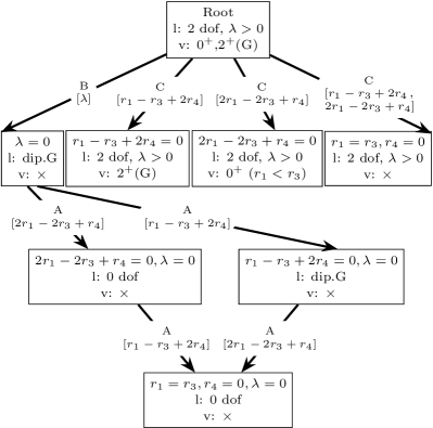
Figure 1: The critical cases of zero-torsion PGT⁺, for which the Lagrangian has the form (56). See the text for details.

IV.2 Zero-curvature PGT⁺

One may impose zero curvature in PGT⁺ (to obtain teleparallel PGT⁺) by setting $A_{AB\mu}=0$ Blagojević (2002), and the corresponding Lagrangian is given by

$$\frac{\mathcal{L}}{b} =\left(\frac{t_{1}}{3}+\frac{t_{2}}{12}\right)\mathcal{T}^{ABC}\mathcal{T}_{ABC}+\left(\!-\frac{t_{1}}{3}+\frac{t_{2}}{6}\right)\mathcal{T}^{ABC}\mathcal{T}_{BCA}$$

$$+\left(\!-\frac{t_{1}}{3}+\frac{2t_{3}}{3}\right)\mathcal{T}\text{}_{B}\text{}_{A}\text{}^{B}\mathcal{T}\text{}_{C}\text{}^{A}\text{}^{C}.$$ (57)

Applying the method described in Sec. III to this case yields the results presented in results Fig. 2, which uses the same conventions as in Fig. 1. We again compare our results with the literature in Sec. IV.4.

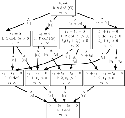
Figure 2: The critical cases of zero-curvature (teleparallel) PGT⁺, for which the Lagrangian has the form (57). See text for details.

IV.3 Full PGT⁺

We now turn our attention back to the general case of full PGT⁺, for which the Lagrangian is given by (49). Starting from the “root” theory, for which no relationship is imposed on the parameters in the Lagrangian, our method outlined in Sec. III systematically identifies 1918 critical cases (excluding the “vanishing” Lagrangian case for which all parameters are zero), which thus cannot be displayed in diagrammatic form such as in Figs 1 and 2. Of these critical cases, we find that 450 can be free of ghosts and tachyons, provided the parameters in each case satisfy some conditions without generating another critical case. The full set of results displayed in an interactive form can be found at: http://www.mrao.cam.ac.uk/projects/gtg/pgt/.

IV.4 Comparison with previous results

We content ourselves here with presenting in Table 1 our results for the root PGT⁺ theory and the small subset of critical cases that have been studied previously in the literature. We also list those critical cases of the torsionless and teleparallel PGT⁺ theories (see Figs. 1 and 2) that have been considered previously in the literature. Overall, we find that our results are indeed consistent with those reported by other authors, apart from a few minor differences that are most likely the result of typographical errors in earlier papers.

Table 1: Conditions for no ghosts or tachyons for the PGT⁺ root theory and a subset of critical cases analyzed previously in the literature. “Massless/massive” denotes the particle content found in the literature, and the parentheses contain the number of degrees of freedom of particles in the massless sector. “Dip. G” means the massless sector contains a dipole ghost. Where our results differ from those in the literature, ours are put in squared brackets. Cells marked with “*” are discussed further in the text, and “-” means the particle content is not mentioned in the cited paper.

#	Paper	Critical Conditions	No-ghost-and-tachyon Conditions	Massless	Massive
1	Sezgin and van Nieuwenhuizen (1980)	$\times$	Ghost (massive)	$2^{+}$ (2)	$0^{-}$,$0^{+}$,$1^{-}$, $1^{+}$,$2^{-}$,$2^{+}$
2	Sezgin and van Nieuwenhuizen (1980)	$t_{1}=t_{2}=t_{3}=r_{1}=r_{2}=r_{3}=r_{4}=r_{5}=0$	$\lambda>0$	$2^{+}$ (2)	$\times$
3	Sezgin and van Nieuwenhuizen (1980)	$t_{1}=-t_{2}=-t_{3}=-\lambda$, $r_{1}=r_{2}=r_{3}=r_{4}=r_{5}=0$	$\lambda>0$	$2^{+}$ (2)	$\times$
4	Sezgin and van Nieuwenhuizen (1980)	$t_{1}=-t_{2}=-t_{3}=-\lambda$, $r_{1}=r_{3}=r_{4}=r_{5}=0$	$\lambda>0,r_{2}<0$	$2^{+}$ (2)	$0^{-}$
5	Sezgin and van Nieuwenhuizen (1980)	$t_{1}=-t_{2},r_{1}=r_{3}$, $r_{4}=r_{2}=0$	$\lambda>0,r_{1}>0[<0]$, $r_{1}+r_{5}>0[<0]$, $t_{1}>0,t_{3}(t_{1}+t_{3})>0$	$2^{+}$ (2)	$1^{-}$, $2^{-}$
6	Sezgin and van Nieuwenhuizen (1980)	$t_{1}=-t_{2},r_{1}=r_{3}$, $r_{4}=r_{2}=0$, torsionless	$\lambda>0$	$2^{+}$ (2)	$\times$
7	Sezgin and van Nieuwenhuizen (1980)	$t_{1}=-t_{3}=-\lambda,r_{1}=0$, $r_{4}=-r_{5}$	$t_{2}>\lambda>0,r_{2}<0$, $2r_{3}+r_{5}>0$	$2^{+}$ (2)	$0^{-}$, $1^{+}$
8	Sezgin and van Nieuwenhuizen (1980)	$t_{1}=-t_{3}=-\lambda,r_{1}=0$, $r_{4}=-r_{5},r_{2}=0$	$2r_{3}+r_{5}>0,\lambda>0$, $t_{2}(t_{2}-\lambda)>0$	$2^{+}$ (2)	$1^{+}$
9	Sezgin and van Nieuwenhuizen (1980)	$t_{1}=-t_{3}=-\lambda,r_{1}=0$, $r_{4}=-r_{5},r_{2}=0$, torsionless	Ghost	-	-
10	Sezgin and van Nieuwenhuizen (1980)	$r_{1}=0,2r_{3}=r_{4}=-r_{5}$	$\lambda>0,r_{2}<0,r_{3}>0,t_{2}>0$, $t_{3}\left(\lambda-t_{3}\right)<0$	$2^{+}$ (2)	$0^{-}$, $0^{+}$
11	Sezgin and van Nieuwenhuizen (1980); Stelle (1978)	$r_{1}=0,2r_{3}=r_{4}=-r_{5}$, torsionless	$\lambda>0,r_{3}>0$	- [(2)]	- $[0^{+}]$
12	Sezgin (1981)	(1)-(12)*	*	$2^{+}$ (2)	*
13	Sezgin (1981)	$t_{1}=t_{2}=t_{3}=0,r_{1}=r_{3}$, $r_{4}=0,2r_{3}+r_{5}=0$	$\lambda>0,r_{1}>0$ $[\lambda>0]$*	$2^{+}$,$1^{-}$* (4) [(2)]	$\times$
14	Kuhfuss and Nitsch (1986)	$t_{1}=t_{2}=t_{3}=0,r_{1}=r_{3}$, $r_{4}=0,2r_{3}+r_{5}=0$	$\lambda>0$*	$2^{+}$ (2)	$\times$
15	Kuhfuss and Nitsch (1986)	$t_{1}=-t_{3}$, teleparallel	$t_{1}+t_{2}>0,t_{1}+\lambda>0$*	$2^{+}$,$0^{+}$ (3)	$\times$
16	Lord and Sinha (1988)	$t_{1}=-t_{3}$, teleparallel	$t_{1}+\lambda>0$	$2^{+}$ (2) $[(3)]$	$\times$
17	Battiti and Tollek (1985)	$r_{4}=-(r_{1}/2)+r_{3}/2,t_{3}=0$	$r_{1}+r_{3}+2r_{5}<0$, $\lambda>0$ (massless)	$2^{+}$,$1$ (4)	-
18	Battiti and Tollek (1985)	$r_{2}=0,t_{2}=0$	$2r_{3}+r_{5}>0,\lambda>0$ (massless)	$2^{+}$,$1$ (4)	-
19	Battiti and Tollek (1985)	$t_{2}=t_{3}=r_{1}-r_{3}+2r_{4}=r_{2}=0$	$2r_{3}+r_{5}>0$, $r_{1}+r_{3}+2r_{5}<0$, $\lambda>0$ (massless)	$2^{+}$,$1$,$1$ (6)	-
20	Stelle (1978)	torsionless	Ghost (massive $2^{+}$)	$2^{+}$ (2)	$0^{+}$,$2^{+}$
21	Biswas et al. (2013); Stelle (1978)	$r_{1}-r_{3}+2r_{4}=0$, torsionless	Ghost (massive $2^{+}$)	$2^{+}$ (2)	$2^{+}$
22	Riegert (1984)	$r_{1}-r_{3}+2r_{4}=\lambda=0$, torsionless	Ghost (massless)	$2^{+}$,$1$,$2^{+}$ (dip. G)*	$\times$

Some of the cases listed in Table 1 are worthy of further discussion, as follows:

• Case 1: This is the “root” PGT⁺ theory, in which no critical condition holds. We find the massless no-ghost condition $\lambda>0$, which agrees with Sezgin and van Nieuwenhuizen (1980). In the massive case, we find the no-tachyon condition in each spin-parity sector to be:

  $$0^{-} :-\frac{t_{2}}{r_{2}}>0$$

  $$0^{+} :\frac{t_{3}\lambda}{2\left(r_{1}-r_{3}+2r_{4}\right)\left(t_{3}-\lambda\right)}>0$$

  $$1^{-} :-\frac{3t_{1}t_{3}}{2\left(r_{1}+r_{4}+r_{5}\right)\left(t_{1}+t_{3}\right)}>0$$

  $$1^{+} :-\frac{3t_{1}t_{2}}{2\left(2r_{3}+r_{5}\right)\left(t_{1}+t_{2}\right)}>0$$

  $$2^{-} :-\frac{t_{1}}{2r_{1}}>0$$

  $$2^{+} :-\frac{t_{1}\lambda}{2\left(2r_{1}-2r_{3}+r_{4}\right)\left(t_{1}+\lambda\right)}>0,$$ (58)

  and the no-ghost condition in each sector is:

  $$0^{-} :-\frac{1}{r_{2}}>0$$

  $$0^{+} :\frac{-r_{1}t_{3}+r_{3}t_{3}-2r_{4}t_{3}-t_{3}\lambda+\lambda^{2}}{2\left(r_{1}-r_{3}+2r_{4}\right)\lambda\left(-t_{3}+\lambda\right)}>0$$

  $$1^{-} :-\frac{3\left(t_{1}^{2}+2t_{3}^{2}\right)}{2\left(r_{1}+r_{4}+r_{5}\right)\left(t_{1}+t_{3}\right){}^{2}}>0$$

  $$1^{+} :\frac{3\left(t_{1}^{2}+2t_{2}^{2}\right)}{2\left(2r_{3}+r_{5}\right)\left(t_{1}+t_{2}\right){}^{2}}>0$$

  $$2^{-} :-\frac{1}{r_{1}}>0$$

  $$2^{+} :\frac{-2r_{1}t_{1}+2r_{3}t_{1}-r_{4}t_{1}+t_{1}\lambda+\lambda^{2}}{\left(2r_{1}-2r_{3}+r_{4}\right)\lambda\left(t_{1}+\lambda\right)}>0.$$ (59)

  These conditions are again equivalent to those in Sezgin and van Nieuwenhuizen (1980), as expected, and cannot be satisfied simultaneously. Hence, the theory contains a massive ghost, as is well known.

• Case 1: This is Einstein–Cartan theory, and our results are consistent with the literature.

• Case 1: Our conditions $\lambda>0,r_{1}<0,r_{1}+r_{5}<0,t_{1}>0,t_{3}(t_{1}+t_{3})>0$ differ from the conditions $\lambda>0,r_{1}>0,r_{1}+r_{5}>0,t_{1}>0,t_{3}(t_{1}+t_{3})>0$ found in Sezgin and van Nieuwenhuizen (1980) in that two of the inequalities have the opposite sign. We believe these are typos in Sezgin and van Nieuwenhuizen (1980).

• Case 1: This torsionless theory corresponds to that in node 4 of row 2 in Fig. 1. We obtain the condition $\lambda>0$, with only 2 massless degrees of freedom, but Sezgin and van Nieuwenhuizen (1980) also set $2t_{3}-t_{1}=3\lambda,r_{5}=0$. These additional conditions neither cause the theory to become a critical case nor contradict the other conditions, so adding them has no effect on the particle content. Sezgin and van Nieuwenhuizen (1980) finds that the action reduces to the Einstein action, which is consistent with our result.

• Case 1: We find that the critical cases that contain three coefficient equations and only type C critical conditions are precisely the 12 cases listed in Table I of Sezgin (1981), and we obtained the same particle content for each theory.

• Case 1: Our no-ghost conditions and massless particle content are different from those found in Sezgin (1981). However, Kuhfuss and Nitsch (1986) studied the same theory and obtained the same conditions and particle content as ours. Moreover, our result that there is no massless propagating tordion in this theory is also found in Blagojević and Vasilić (1987). We notice that, compared to our analysis, some terms in Eq. (8) in Sezgin (1981) have different signs, which we believe to be typos.

• Case 1 and 1: We find that there is an overall sign difference between our linearized Lagrangian and that in Kuhfuss and Nitsch (1986), so the conditions also have an overall sign difference. We assume that this is a minor error either in their calculation or our conversion of it to our notation. We have thus added an overall minus sign to their conditions.

• Case 1: This theory was also studied in Lord and Sinha (1988) (along with Case 1), who found only a spin-2 massless mode with the condition $t_{1}+\lambda>0$. However, they studied only the spin-2 particles, so our results are consistent.

• Case 1: We believe that the condition $\alpha-\gamma_{3}=0$ quoted in Battiti and Tollek (1985) contains a typo and should instead read $\alpha-\gamma_{3}\neq 0$, which is equivalent to $t_{1}=0\to t_{1}\neq 0$ in our notation, thus yielding our result.

• Case 1: This is conformal gravity. Riegert (1984) showed it has a normal spin-2, a normal spin-1, and a ghost spin-2 mode, all massless. We find there is no massive mode, and there must be dipole ghost(s) in the massless sector. Our method can determine the existence of ghosts, but not the degrees of freedom in the massless sector if there are dipole ghost(s). Nonetheless, the results are consistent.

IV.5 Source constraints

As mentioned previously, if the parameters in the PGT⁺ Lagrangian (49) satisfy some specific conditions (type A critical cases), then the resulting theory may possess extra gauge invariances beyond the Poincaré symmetry assumed in its construction. For example, for Case 1 in Table 1, it is noted in Sezgin (1981); Kuhfuss and Nitsch (1986) that the theory is additionally invariant under the gauge transformation

$$\delta A_{ABC} =\partial_{A}\Lambda_{BC}-\partial_{B}\Lambda_{AC}+\partial_{C}\theta_{AB},$$ (60)

where $\partial^{B}\Lambda_{AB}=0$, $\theta_{AB}=\partial_{A}V_{B}-\partial_{B}V_{A}$, $\partial^{A}V_{A}=0$ and $\Lambda$ and $V$ are arbitrary (see also Blagojević and Vasilić (1987)), and has the additional source constraints

$$\partial^{B}\tau_{ABC} =0,\qquad\partial^{C}\tau_{ABC}=0,$$ (61)

beyond the standard ones $\partial^{B}\sigma_{AB}=0$ and $\sigma_{[AB]}+\partial^{C}\tau_{ABC}=0$ arising from the Poincaré symmetry. Here, $\sigma_{AB}$ and $\tau_{ABC}$ are the source currents of the $f_{AB}$ (graviton) and $A_{ABC}$ (tordion) gravitational fields, respectively.

Our approach also found the same source constraints for this theory, although not directly as tensor equations, but instead in component form for $k$ aligned with the $z$-direction. Indeed, we found there are 310 different sets of source constraints among the root PGT⁺ theory and its 1918 critical cases. We are not able to convert all of them automatically into their corresponding tensor equations, but it is possible to make such a conversion in some cases. This is performed by first suggesting possible tensor equations from the patterns present in the component equations, then converting the possible tensor equations into component forms, and finally comparing whether they are equivalent. In LABEL:tab:someSC, we present the results for all the sets of sources constraints that we were able to convert into tensor form. We find that the same set of source constraints may hold for more than one critical case, so in the table we list only the case having the simplest critical conditions. It is worth noting that the first case listed is the root PGT⁺ theory, for which we recover the two well-known source constraints arising from the Poincaré symmetry alone. We also note that, aside from the root theory, the numbering of cases in the table is not related to that used in table 1.

Table 2: Source constraints for the root PGT⁺ theory and those critical cases for which the constraints could be found in tensor form. Note that there may be more than one critical case sharing the same source constraints, so we list only the case having the simplest critical conditions. The numbering of cases is not related to that used in Table 1.

#	Critical Conditions	Source constraints
1	$\times$	$k\text{}^{B}\sigma\text{}_{AB}=\sigma\text{}_{AB}-\sigma\text{}_{BA}+2ik\text{}^{C}\tau\text{}_{ABC}=0$
2	$r_{1}-r_{3}=r_{4}=\lambda=0$	$i\sigma\text{}_{AB}+i\sigma\text{}_{BA}-2k\text{}^{C}\tau\text{}_{CAB}-2k\text{}^{C}\tau\text{}_{CBA}=i\sigma\text{}_{AB}-i\sigma\text{}_{BA}-2k\text{}^{C}\tau\text{}_{ABC}=0$
3	$r_{1}/2-r_{3}/2+r_{4}=r_{1}/2+r_{3}/2+r_{5}=t_{3}=0$	$k\text{}^{B}\sigma\text{}_{AB}=\sigma\text{}_{AB}-\sigma\text{}_{BA}+2ik\text{}^{C}\tau\text{}_{ABC}=g\text{}^{BC}\tau\text{}_{ACB}=0$
4	$r_{1}/2-r_{3}/2+r_{4}=r_{1}/2+r_{3}/2+r_{5}=t_{1}=t_{3}=0$	$k\text{}^{B}\sigma\text{}_{AB}=\sigma\text{}_{AB}-\sigma\text{}_{BA}+2ik\text{}^{C}\tau\text{}_{ABC}=k\text{}^{B}\sigma\text{}_{BA}=g\text{}^{BC}\tau\text{}_{ACB}=0$
5	$r_{1}=r_{3}=r_{4}=r_{5}=t_{1}=t_{3}=0$	$k\text{}^{B}\sigma\text{}_{AB}=\sigma\text{}_{AB}-\sigma\text{}_{BA}-2ik\text{}^{C}\tau\text{}_{CBA}=\tau\text{}_{ACB}+\tau\text{}_{BCA}=0$
6	$r_{1}=r_{3}=r_{4}=r_{5}=t_{1}=t_{2}=t_{3}=0$	$k\text{}^{B}\sigma\text{}_{AB}=\sigma\text{}_{AB}-\sigma\text{}_{BA}=k\text{}^{C}\tau\text{}_{CBA}=\tau\text{}_{ACB}+\tau\text{}_{BCA}=0$
7	$r_{1}=r_{3}=r_{4}=r_{5}=t_{1}=t_{2}=t_{3}=\lambda=0$	$\sigma\text{}_{AB}=k\text{}^{C}\tau\text{}_{CBA}=\tau\text{}_{ACB}+\tau\text{}_{BCA}=0$
8	$r_{1}=r_{2}=r_{3}=r_{4}=r_{5}=t_{1}=t_{2}=t_{3}=0$	$k\text{}^{B}\sigma\text{}_{AB}=\sigma\text{}_{AB}-\sigma\text{}_{BA}=\tau\text{}_{BCA}=0$
9	$r_{1}=r_{3}=r_{4}=r_{5}=t_{1}=t_{3}=\lambda=0$	$\sigma\text{}_{AB}-ik\text{}^{C}\tau\text{}_{CBA}=\tau\text{}_{ACB}+\tau\text{}_{BCA}=0$
10	$r_{1}/3-r_{3}=r_{1}/3+r_{4}=2r_{1}/3+r_{5}=t_{1}=t_{3}=0$	$k\text{}^{B}\sigma\text{}_{AB}=\sigma\text{}_{AB}-\sigma\text{}_{BA}+ik\text{}^{C}\tau\text{}_{CAB}-ik\text{}^{C}\tau\text{}_{CBA}=g\text{}^{BC}\tau\text{}_{ACB}=2k\text{}^{C}\tau\text{}_{ABC}-k\text{}^{C}\tau\text{}_{CAB}+k\text{}^{C}\tau\text{}_{CBA}=0$
11	$r_{1}/3-r_{3}=r_{1}/3+r_{4}=2r_{1}/3+r_{5}=t_{1}=t_{2}=t_{3}=0$	$k\text{}^{B}\sigma\text{}_{AB}=\sigma\text{}_{AB}-\sigma\text{}_{BA}=g\text{}^{BC}\tau\text{}_{ACB}=k\text{}^{C}\tau\text{}_{CAB}-k\text{}^{C}\tau\text{}_{CBA}=k\text{}^{C}\tau\text{}_{ABC}=0$
12	$r_{2}=r_{1}/3-r_{3}=r_{1}/3+r_{4}=2r_{1}/3+r_{5}=t_{1}=t_{2}=t_{3}=0$	$k\text{}^{B}\sigma\text{}_{AB}=\sigma\text{}_{AB}-\sigma\text{}_{BA}=g\text{}^{BC}\tau\text{}_{ACB}=k\text{}^{C}\tau\text{}_{CAB}-k\text{}^{C}\tau\text{}_{CBA}=\tau\text{}_{ABC}-\tau\text{}_{ACB}+\tau\text{}_{BCA}=0$
13	$r_{2}=r_{1}/3-r_{3}=r_{1}/3+r_{4}=2r_{1}/3+r_{5}=t_{1}=t_{2}=t_{3}=\lambda=0$	$\sigma\text{}_{AB}=g\text{}^{BC}\tau\text{}_{ACB}=k\text{}^{C}\tau\text{}_{CAB}-k\text{}^{C}\tau\text{}_{CBA}=\tau\text{}_{ABC}-\tau\text{}_{ACB}+\tau\text{}_{BCA}=0$
14	$r_{1}/3-r_{3}=r_{1}/3+r_{4}=2r_{1}/3+r_{5}=t_{1}=t_{2}=t_{3}=\lambda=0$	$\sigma\text{}_{AB}=g\text{}^{BC}\tau\text{}_{ACB}=k\text{}^{C}\tau\text{}_{CAB}-k\text{}^{C}\tau\text{}_{CBA}=k\text{}^{C}\tau\text{}_{ABC}=0$
15	$r_{1}/3-r_{3}=r_{1}/3+r_{4}=2r_{1}/3+r_{5}=t_{1}=t_{3}=\lambda=0$	$\sigma\text{}_{AB}+ik\text{}^{C}\tau\text{}_{ABC}=g\text{}^{BC}\tau\text{}_{ACB}=2i\sigma\text{}_{AB}-k\text{}^{C}\tau\text{}_{CAB}+k\text{}^{C}\tau\text{}_{CBA}=0$
16	$r_{1}-r_{3}=r_{4}=r_{1}+r_{5}=t_{1}=t_{2}=t_{3}=\lambda=0$	$\sigma\text{}_{AB}=g\text{}^{BC}\tau\text{}_{ACB}=k\text{}^{C}\tau\text{}_{CAB}+k\text{}^{C}\tau\text{}_{CBA}=k\text{}^{C}\tau\text{}_{ABC}=0$
17	$r_{1}-r_{3}=r_{4}=r_{1}+r_{5}=t_{1}=t_{3}=0$	$k\text{}^{B}\sigma\text{}_{AB}=\sigma\text{}_{AB}-\sigma\text{}_{BA}+2ik\text{}^{C}\tau\text{}_{ABC}=g\text{}^{BC}\tau\text{}_{ACB}=k\text{}^{C}\tau\text{}_{CAB}+k\text{}^{C}\tau\text{}_{CBA}=0$
18	$r_{1}-r_{3}=r_{4}=r_{1}+r_{5}=t_{1}=t_{3}=\lambda=0$	$\sigma\text{}_{AB}+ik\text{}^{C}\tau\text{}_{ABC}=g\text{}^{BC}\tau\text{}_{ACB}=k\text{}^{C}\tau\text{}_{CAB}+k\text{}^{C}\tau\text{}_{CBA}=0$
19	$r_{1}-r_{3}=r_{4}=r_{1}+r_{5}=t_{1}=t_{2}=t_{3}=0$	$k\text{}^{B}\sigma\text{}_{AB}=\sigma\text{}_{AB}-\sigma\text{}_{BA}=g\text{}^{BC}\tau\text{}_{ACB}=k\text{}^{C}\tau\text{}_{CAB}+k\text{}^{C}\tau\text{}_{CBA}=k\text{}^{C}\tau\text{}_{ABC}=0$
20	$r_{1}/2-r_{3}/2+r_{4}=r_{1}/2+r_{3}/2+r_{5}=t_{1}=t_{2}=t_{3}=0$	$k\text{}^{B}\sigma\text{}_{AB}=\sigma\text{}_{AB}-\sigma\text{}_{BA}=g\text{}^{BC}\tau\text{}_{ACB}=k\text{}^{C}\tau\text{}_{ABC}=0$
21	$r_{2}=r_{1}-r_{3}=r_{4}=2r_{1}+r_{5}=t_{1}=t_{2}=t_{3}=\lambda=0$	$\sigma\text{}_{AB}=k\text{}^{C}\tau\text{}_{CBA}=\tau\text{}_{ABC}-\tau\text{}_{ACB}+\tau\text{}_{BCA}=0$
22	$r_{1}/2-r_{3}/2+r_{4}=r_{1}/2+r_{3}/2+r_{5}=t_{1}=t_{2}=t_{3}=\lambda=0$	$\sigma\text{}_{AB}=g\text{}^{BC}\tau\text{}_{ACB}=k\text{}^{C}\tau\text{}_{ABC}=0$
23	$r_{1}-r_{3}=r_{4}=2r_{1}+r_{5}=t_{1}=t_{2}=t_{3}=\lambda=0$	$\sigma\text{}_{AB}=k\text{}^{C}\tau\text{}_{CBA}=k\text{}^{C}\tau\text{}_{ABC}=0$
24	$r_{1}/2-r_{3}/2+r_{4}=r_{1}/2+r_{3}/2+r_{5}=t_{1}=t_{3}=\lambda=0$	$k\text{}^{B}\sigma\text{}_{AB}=g\text{}^{BC}\tau\text{}_{ACB}=i\sigma\text{}_{AB}-k\text{}^{C}\tau\text{}_{ABC}=0$
25	$r_{1}-r_{3}=r_{4}=2r_{1}+r_{5}=t_{1}=t_{3}=\lambda=0$	$\sigma\text{}_{AB}-ik\text{}^{C}\tau\text{}_{CBA}=2\sigma\text{}_{AB}+ik\text{}^{C}\tau\text{}_{ABC}+ik\text{}^{C}\tau\text{}_{CAB}=0$
26	$r_{1}-r_{3}=r_{4}=r_{1}+r_{5}=t_{3}=\lambda=0$	$g\text{}^{BC}\tau\text{}_{ACB}=i\sigma\text{}_{AB}+i\sigma\text{}_{BA}-2k\text{}^{C}\tau\text{}_{CAB}-2k\text{}^{C}\tau\text{}_{CBA}=i\sigma\text{}_{AB}-i\sigma\text{}_{BA}-2k\text{}^{C}\tau\text{}_{ABC}=0$
27	$r_{1}-r_{3}=r_{4}=t_{1}=t_{2}=t_{3}=\lambda=0$	$\sigma\text{}_{AB}=k\text{}^{C}\tau\text{}_{CAB}+k\text{}^{C}\tau\text{}_{CBA}=k\text{}^{C}\tau\text{}_{ABC}=0$
28	$r_{1}=r_{3}=r_{4}=r_{5}=t_{2}=t_{3}=\lambda=0$	$\sigma\text{}_{AB}+2ik\text{}^{C}\tau\text{}_{CBA}=\sigma\text{}_{AB}+2ik\text{}^{C}\tau\text{}_{ABC}+2ik\text{}^{C}\tau\text{}_{CAB}=g\text{}^{BC}\tau\text{}_{ACB}=0$
29	$r_{1}-r_{3}=r_{4}=t_{1}=t_{3}=\lambda=0$	$k\text{}^{C}\tau\text{}_{CAB}+k\text{}^{C}\tau\text{}_{CBA}=i\sigma\text{}_{AB}-k\text{}^{C}\tau\text{}_{ABC}=0$
30	$r_{1}=r_{2}=r_{3}=r_{4}=r_{5}=t_{2}=t_{3}=\lambda=0$	$\sigma\text{}_{AB}+2ik\text{}^{C}\tau\text{}_{CBA}=g\text{}^{BC}\tau\text{}_{ACB}=\tau\text{}_{ABC}-\tau\text{}_{ACB}+\tau\text{}_{BCA}=0$
31	$r_{2}=r_{1}-r_{3}=r_{4}=2r_{1}+r_{5}=t_{2}=\lambda=0$	$\sigma\text{}_{AB}+2ik\text{}^{C}\tau\text{}_{CBA}=\tau\text{}_{ABC}-\tau\text{}_{ACB}+\tau\text{}_{BCA}=0$
32	$r_{1}-r_{3}=r_{4}=2r_{1}+r_{5}=t_{2}=\lambda=0$	$\sigma\text{}_{AB}+2ik\text{}^{C}\tau\text{}_{CBA}=\sigma\text{}_{AB}+2ik\text{}^{C}\tau\text{}_{ABC}+2ik\text{}^{C}\tau\text{}_{CAB}=0$
33	$r_{2}=r_{1}/3-r_{3}=r_{1}/3+r_{4}=2r_{1}/3+r_{5}=t_{2}=t_{3}=0$	$k\text{}^{B}\sigma\text{}_{AB}=\sigma\text{}_{AB}-\sigma\text{}_{BA}-2ik\text{}^{C}\tau\text{}_{CAB}+2ik\text{}^{C}\tau\text{}_{CBA}=g\text{}^{BC}\tau\text{}_{ACB}=\tau\text{}_{ABC}-\tau\text{}_{ACB}+\tau\text{}_{BCA}=0$
34	$r_{1}/3-r_{3}=r_{1}/3+r_{4}=2r_{1}/3+r_{5}=t_{2}=t_{3}=0$	$k\text{}^{B}\sigma\text{}_{AB}=\sigma\text{}_{AB}-\sigma\text{}_{BA}-2ik\text{}^{C}\tau\text{}_{CAB}+2ik\text{}^{C}\tau\text{}_{CBA}=\sigma\text{}_{AB}-\sigma\text{}_{BA}+2ik\text{}^{C}\tau\text{}_{ABC}=g\text{}^{BC}\tau\text{}_{ACB}=0$
35	$r_{1}-r_{3}=r_{4}=t_{1}=t_{3}=0$	$k\text{}^{B}\sigma\text{}_{AB}=\sigma\text{}_{AB}-\sigma\text{}_{BA}+2ik\text{}^{C}\tau\text{}_{ABC}=k\text{}^{C}\tau\text{}_{CAB}+k\text{}^{C}\tau\text{}_{CBA}=0$
36	$r_{1}-r_{3}=r_{4}=2r_{1}+r_{5}=t_{1}=t_{3}=0$	$k\text{}^{B}\sigma\text{}_{AB}=\sigma\text{}_{AB}-\sigma\text{}_{BA}-2ik\text{}^{C}\tau\text{}_{CBA}=\sigma\text{}_{AB}-\sigma\text{}_{BA}+ik\text{}^{C}\tau\text{}_{ABC}+ik\text{}^{C}\tau\text{}_{CAB}=0$
37	$r_{1}-r_{3}=r_{4}=2r_{1}+r_{5}=t_{1}=t_{2}=t_{3}=0$	$k\text{}^{B}\sigma\text{}_{AB}=\sigma\text{}_{AB}-\sigma\text{}_{BA}=k\text{}^{C}\tau\text{}_{CBA}=k\text{}^{C}\tau\text{}_{ABC}=0$
38	$r_{2}=r_{1}-r_{3}=r_{4}=2r_{1}+r_{5}=t_{1}=t_{2}=t_{3}=0$	$k\text{}^{B}\sigma\text{}_{AB}=\sigma\text{}_{AB}-\sigma\text{}_{BA}=k\text{}^{C}\tau\text{}_{CBA}=\tau\text{}_{ABC}-\tau\text{}_{ACB}+\tau\text{}_{BCA}=0$
39	$r_{1}-r_{3}=r_{4}=t_{1}=t_{2}=t_{3}=0$	$k\text{}^{B}\sigma\text{}_{AB}=\sigma\text{}_{AB}-\sigma\text{}_{BA}=k\text{}^{C}\tau\text{}_{CAB}+k\text{}^{C}\tau\text{}_{CBA}=k\text{}^{C}\tau\text{}_{ABC}=0$
40	$r_{2}=2r_{3}+r_{5}=t_{1}=t_{2}=t_{3}=\lambda=0$	$\sigma\text{}_{AB}=\tau\text{}_{ABC}-\tau\text{}_{ACB}+\tau\text{}_{BCA}=k\text{}^{C}\tau\text{}_{CAB}-k\text{}^{C}\tau\text{}_{CBA}=0$
41	$t_{1}=t_{3}=0$	$k\text{}^{B}\sigma\text{}_{AB}=\sigma\text{}_{AB}-\sigma\text{}_{BA}+2ik\text{}^{C}\tau\text{}_{ABC}=k\text{}^{B}\sigma\text{}_{BA}=0$
42	$2r_{3}+r_{5}=t_{1}=t_{2}=t_{3}=\lambda=0$	$\sigma\text{}_{AB}=k\text{}^{C}\tau\text{}_{CAB}-k\text{}^{C}\tau\text{}_{CBA}=k\text{}^{C}\tau\text{}_{ABC}=0$
43	$r_{2}=2r_{3}+r_{5}=t_{1}=t_{2}=t_{3}=0$	$k\text{}^{B}\sigma\text{}_{AB}=\sigma\text{}_{AB}-\sigma\text{}_{BA}=\tau\text{}_{ABC}-\tau\text{}_{ACB}+\tau\text{}_{BCA}=k\text{}^{C}\tau\text{}_{CAB}-k\text{}^{C}\tau\text{}_{CBA}=0$
44	$2r_{3}+r_{5}=t_{1}=t_{3}=\lambda=0$	$3i\sigma\text{}_{AB}-k\text{}^{C}\tau\text{}_{ABC}-k\text{}^{C}\tau\text{}_{CAB}+k\text{}^{C}\tau\text{}_{CBA}=2i\sigma\text{}_{AB}-k\text{}^{C}\tau\text{}_{CAB}+k\text{}^{C}\tau\text{}_{CBA}=0$
45	$2r_{3}+r_{5}=t_{1}=t_{3}=0$	$k\text{}^{B}\sigma\text{}_{AB}=\sigma\text{}_{AB}-\sigma\text{}_{BA}+ik\text{}^{C}\tau\text{}_{CAB}-ik\text{}^{C}\tau\text{}_{CBA}=\sigma\text{}_{AB}-\sigma\text{}_{BA}+2ik\text{}^{C}\tau\text{}_{ABC}=0$
46	$2r_{3}+r_{5}=t_{1}=t_{2}=t_{3}=0$	$k\text{}^{B}\sigma\text{}_{AB}=\sigma\text{}_{AB}-\sigma\text{}_{BA}=k\text{}^{C}\tau\text{}_{CAB}-k\text{}^{C}\tau\text{}_{CBA}=k\text{}^{C}\tau\text{}_{ABC}=0$
47	$t_{1}=t_{2}=t_{3}=0$	$k\text{}^{B}\sigma\text{}_{AB}=\sigma\text{}_{AB}-\sigma\text{}_{BA}=k\text{}^{C}\tau\text{}_{ABC}=0$
48	$t_{1}=t_{2}=t_{3}=\lambda=0$	$\sigma\text{}_{AB}=k\text{}^{C}\tau\text{}_{ABC}=0$
49	$t_{1}=t_{3}=\lambda=0$	$k\text{}^{B}\sigma\text{}_{AB}=i\sigma\text{}_{AB}-k\text{}^{C}\tau\text{}_{ABC}=0$
50	$r_{2}=2r_{3}+r_{5}=t_{2}=0$	$k\text{}^{B}\sigma\text{}_{AB}=\sigma\text{}_{AB}-\sigma\text{}_{BA}-2ik\text{}^{C}\tau\text{}_{CAB}+2ik\text{}^{C}\tau\text{}_{CBA}=\tau\text{}_{ABC}-\tau\text{}_{ACB}+\tau\text{}_{BCA}=0$
51	$2r_{3}+r_{5}=t_{2}=0$	$k\text{}^{B}\sigma\text{}_{AB}=\sigma\text{}_{AB}-\sigma\text{}_{BA}-2ik\text{}^{C}\tau\text{}_{CAB}+2ik\text{}^{C}\tau\text{}_{CBA}=i\sigma\text{}_{AB}-i\sigma\text{}_{BA}-2k\text{}^{C}\tau\text{}_{ABC}=0$

IV.6 Power-counting renormalizability

Table 3: PC renormalizable critical cases that are ghost and tachyon free and have only massless propagating modes. “Additional condition” are the conditions that prevent the theory becoming a different critical case. The column “$b$ sectors” describes the elements in the $b^{-1}$-matrix of each spin-parity sector in the sequence $(0^{-},0^{+},1^{-},1^{+},2^{-},2^{+})$. Here and in Table 4 it is notated as $\varphi^{n}_{v}$ or $\varphi^{n}_{l}$, where $\varphi$ is the field, $-n$ is the power of $k$ in the element in the $b^{-1}$-matrix, $v$ means massive mode, and $l$ means massless mode.

No.	Critical condition	Additional condition	No-ghost-and-tachyon condition	Massless mode d.o.f.	$b$ sectors
1	$r_{3}=r_{1},r_{2}=r_{4}=$ $t_{1}=t_{2}=t_{3}=\lambda=0$	$r_{1}\neq 0,r_{1}+r_{5}\neq 0$, $2r_{1}+r_{5}\neq 0$	$r_{1}\left(r_{1}+r_{5}\right)\left(2r_{1}+r_{5}\right)<0$	2	$(\times,\times,A_{l}^{2},A_{l}^{2},A_{l}^{2},\times)$
2	$r_{4}=-2r_{1}+2r_{3},r_{2}=$ $t_{1}=t_{2}=t_{3}=\lambda=0$	$r_{3}\neq 0,2r_{3}+r_{5}\neq 0$, $r_{3}+2r_{5}\neq 0,r_{2}\neq 0$	$r_{1}\left(r_{1}-2r_{3}-r_{5}\right)\left(2r_{3}+r_{5}\right)>0$	2	$(\times,A_{l}^{2},A_{l}^{2},A_{l}^{2},A_{l}^{2},\times)$
3	$r_{4}=r_{3}/2,r_{1}=r_{2}=$ $t_{1}=t_{2}=t_{3}=\lambda=0$	$r_{3}\neq 0,2r_{3}+r_{5}\neq 0$, $r_{3}+2r_{5}\neq 0$	$r_{3}\left(2r_{3}+r_{5}\right)\left(r_{3}+2r_{5}\right)<0$	2	$(\times,\times,A_{l}^{2},A_{l}^{2},\times,A_{l}^{2})$
4	$r_{4}=r_{3}/2,r_{1}=$ $t_{1}=t_{2}=t_{3}=\lambda=0$	$r_{3}\neq 0,2r_{3}+r_{5}\neq 0$, $r_{3}+2r_{5}\neq 0,r_{2}\neq 0$	$r_{3}\left(2r_{3}+r_{5}\right)\left(r_{3}+2r_{5}\right)<0$	2	$(A_{l}^{2},\times,A_{l}^{2},A_{l}^{2},\times,A_{l}^{2})$

Table 4: PC renormalizable critical cases that are ghost and tachyon free and have only massive propagating modes. The “$|$” notation denotes the different form of the elements of the $b^{-1}$-matrices in different choices of gauge fixing. The other columns are the same as in Table 3. Note that while there are some $A^{0}$, $s^{2}_{l}$ or $a^{2}_{l}$ in the $b^{-1}$-matrices, the $A^{0}$ terms are not propagating. The $s^{2}_{l}$ or $a^{2}_{l}$ terms may lead to PC nonrenormalizability, but after applying the source constraints and summing all terms from all spin-parity sectors, none of the theories below has a massless propagating mode. Hence, these terms do not affect PC renormalizability.

No.	Critical condition	Additional condition	No-ghost-and-tachyon condition	Massive mode	$b$ sectors
5	$r_{1}=r_{3}=r_{4}=$ $r_{5}=t_{1}=\lambda=0$	$r_{2}\neq 0,t_{2}\neq 0,t_{3}\neq 0$	$t_{2}>0,r_{2}<0$	$0^{-}$	$(A_{v}^{2},A^{0}|s^{2}_{l},A^{0}|s^{2}_{l}|a^{2}_{l},A^{0}|a^{2}_{l},$ $\times,\times)$
6	$r_{1}=r_{3}=r_{4}=$ $r_{5}=t_{1}=t_{3}=\lambda=0$	$r_{2}\neq 0,t_{2}\neq 0$	$t_{2}>0,r_{2}<0$	$0^{-}$	$(A_{v}^{2},\times,\times,A^{0}|a^{2}_{l},\times,\times)$
7	$r_{3}=r_{1},r_{5}=-2r_{1}$, $r_{4}=t_{1}=t_{3}=\lambda=0$	$r_{1}\neq 0,r_{2}\neq 0,t_{2}\neq 0$	$t_{2}>0,r_{2}<0$	$0^{-}$	$(A_{v}^{2},A^{0},\times,A^{0}|a^{2}_{l},\times,\times)$
8	$r_{4}=2r_{3},r_{5}=-2r_{3}$, $r_{1}=t_{1}=t_{3}=\lambda=0$	$r_{2}\neq 0,r_{3}\neq 0,t_{2}\neq 0$	$t_{2}>0,r_{2}<0$	$0^{-}$	$(A_{v}^{2},\times,A_{l}^{2},A^{0},A_{l}^{2},\times)$
9	$r_{4}=r_{3}/2,r_{5}=-2r_{3}$, $r_{1}=t_{1}=t_{3}=\lambda=0$	$r_{2}\neq 0,r_{3}\neq 0,t_{2}\neq 0$	$t_{2}>0,r_{2}<0$	$0^{-}$	$(A_{v}^{2},\times,A_{l}^{2},A^{0}|a^{2}_{l},\times,A_{l}^{2})$
10	$r_{4}=2r_{3}-2r_{1},r_{5}=-2r_{3}$, $t_{1}=t_{3}=\lambda=0$	$r_{1}\neq 0,r_{2}\neq 0$, $r_{1}-r_{3}\neq 0,t_{2}\neq 0$	$t_{2}>0,r_{2}<0$	$0^{-}$	$(A_{v}^{2},A_{l}^{2},A_{l}^{2},A^{0}|a^{2}_{l},A_{l}^{2},\times)$

In addition to possessing no ghosts or tachyons, a healthy physical theory should also be renormalizable. The first step in assessing whether this is possible is to determine whether the theory is power-counting (PC) renormalizable.

Even this condition can be quite difficult to establish in the general case in which the propagator for the theory contains terms that mix different fields, which is the case for PGT⁺. Nonetheless, in the decomposition of the propagator using SPOs, there are some critical cases for which the mixing terms in the $b$-matrices vanish. In these cases, the physical meaning is much clearer. We therefore focus only on the PGT⁺ critical cases that satisfy this property.

In such cases, one can determine the behavior of the saturated propagator of the $f$ (graviton) and $A$ (tordion) fields when $k^{2}\rightarrow\infty$ by studying the corresponding diagonal elements in the $b$-matrices. If one requires PC renormalizability, the propagator of the graviton should go as $k^{-4}$ and that of the tordion should go as $k^{-2}$ when $k^{2}\rightarrow\infty$ Sezgin and van Nieuwenhuizen (1980). We found 10 PC renormalizable critical cases without ghosts and tachyons, of which four have only massless propagating particles (see table 3) and the remaining six have only a massive propagating mode (see Table 4).

It is possible to use different gauge fixing so that sometimes a graviton mode is transformed to a tordion mode and vice-versa. We find in these PGT⁺ cases, however, gauge fixing does not affect renormalizability. The four cases with only massless modes in Table 3 all contain 2 massless degrees of freedom. There is no way to fix the gauge in these cases without fixing all the graviton degrees of freedom, so they contain only tordions. Nonetheless, we note that the inverse $b$-matrices for cases 3 and 4 have elements in the $2^{+}$ sector, and it might therefore be of interest to investigate their phenomenology further. The six cases in Table 4 all propagate only a massive $0^{-}$ tordion mode and no massless mode, so they are of limited physical interest.

We also investigated the PGT⁺ theories with either zero torsion or zero curvature, discussed in Secs. IV.1 and IV.2 respectively, but found that no cases are both unitary and PC renormalizable.

V Discussion and Conclusions

We have presented a systematic method for obtaining the no-ghost-and-tachyon conditions for all critical cases of a parity-preserving gauge theory of gravity. We have implemented the method as a computer program and examined the critical cases of PGT⁺, as well as of torsionless PGT⁺ and teleparallel PGT⁺. In comparing our results with the literature for the (small) subset of critical cases that have been analyzed previously, we find that they are consistent, apart from a few minor differences that most probably arise from typographical errors in previous works.

Our method does, however, have the shortcoming that it does not yield the spins or parities of the massless particles, but only their total number of degrees of freedom (when there is no dipole ghost). Moreover, in the presence of a dipole ghost, our method can determine only that the dipole ghost exists, but does not yield the number of degrees of freedom.

Although not a shortcoming of our method per se, it is also difficult to classify the results obtained. In particular, care must be taken since, for a given ghost and tachyon free critical case, it is not guaranteed that all of its child critical cases do not contain ghosts or tachyons. Furthermore, in general, a theory has multiple child critical theories, and it also has multiple parent theories, so it is difficult to divide the theories into some categories without cutting lots of relations between parent and child theories. Our interactive interface available at http://www.mrao.cam.ac.uk/projects/gtg/pgt/ is intended to assist in navigating this space of theories.

An alternative method to that presented here is the Hamiltonian approach, which has recently been used to study the particle spectrum of parity-violating PGT by Blagojević and Cvetković Blagojević and Cvetković (2018). Their results can be straightforwardly reduced to PGT⁺ by setting all the $\bar{a}$ and $\bar{b}$ to zero in their paper. This will not cause any new “critical parameters” to vanish. By comparing their “critical parameters” with our “critical conditions,” we find that our type C critical conditions are identical to their critical parameters. These critical parameters are second class constraints Blagojević and Nikolić (1983); Nikolić (1984), so they do not lead to additional gauge invariance, which is consistent with our definition of type C critical cases. As for the type A critical conditions, we believe that they correspond to first class if-constraints because first class constraints represent additional gauge invariance. In Blagojevic’s book Blagojević (2002), the critical parameters for the most general teleparallel PGT⁺ are listed, and found to be first class. Our method found 4 type A conditions from the theory, which is the same as Blagojevic. This is consistent with our supposition. As for the type B critical cases, however, Blagojević and Cvetković (2018) does not mention its consequences (massive particle becomes massless), but only requires the mass squares to be positive. Blagojević and Vasilić Blagojević and Vasilić (1987) studied what happens when massive modes becomes massless. In particular, they claim that if any massive tordion becomes massless, there will be extra gauge invariance. However, in their analysis they always include other critical condition(s) in addition to setting the mass to zero to make the theory healthy, so they are not purely applying type B conditions. It is possible that we combine some type B conditions with some other conditions to get a type A condition and extra gauge invariance appears, so their conclusion does not conflict with ours.

In the context of PGT⁺, it may be of interest to investigate further the theories listed in Table 3, which are both unitary and power-counting renormalizable, and possess only massless propagating particles. Although these theories contain no graviton, only tordions, they may provide some insights into the construction of a self-consistent quantum theory of long-range gravitational interactions. In particular, cases 3 and 4 might be of interest, since they may possess particles in the $2^{+}$ sector. Indeed, it is worth noting that in the absence of torsion the action for both of these cases reduces to that of conformal gravity, which is PC renormalizable but not unitary, as discussed in Case 1 in Sec. IV.4.

Finally, although we demonstrated our method only for PGT⁺ in this paper, it may be applied to more complex theories such as Weyl gauge theory (WGT) Bregman (1973); *Charap1974; *Kasuya1975 or extended Weyl gauge theory (eWGT) Lasenby and Hobson (2016). It is also applicable to conventional metric theories such as $\mathcal{R}^{2}$ theories. We plan to explore its application to such theories in future work.

Appendix A SPIN PROJECTION OPERATORS FOR PGT⁺

The block matrices $\mathsf{P}(J^{P})$ containing the spin projection operators for PGT⁺ used in this paper are as follows (see Sec. II for details):

$$\mathsf{P}\left(0^{-}\right)=\bordermatrix{~{}&A_{ABC}\cr A^{*}_{IJK}&\frac{2}{3}\Theta\text{}_{I}\text{}_{C}\Theta\text{}_{J}\text{}_{A}\Theta\text{}_{K}\text{}_{B}+\frac{1}{3}\Theta\text{}_{I}\text{}_{A}\Theta\text{}_{J}\text{}_{B}\Theta\text{}_{K}\text{}_{C}\cr},$$ (62)

$$\mathsf{P}\left(0^{+}\right)=\bordermatrix{~{}&A_{ABC}&s_{AB}&s_{AB}\cr A^{*}_{IJK}&\frac{2}{3}\Theta\text{}_{C}\text{}_{B}\Theta\text{}_{K}\text{}_{J}\Omega\text{}_{I}\text{}_{A}&\frac{\sqrt{2}}{3}\tilde{k}\text{}_{J}\Theta\text{}_{A}\text{}_{B}\Theta\text{}_{K}\text{}_{I}&\sqrt{\frac{2}{3}}\tilde{k}\text{}_{J}\Theta\text{}_{K}\text{}_{I}\Omega\text{}_{B}\text{}_{A}\cr s^{*}_{IJ}&\frac{\sqrt{2}}{3}\tilde{k}\text{}_{B}\Theta\text{}_{C}\text{}_{A}\Theta\text{}_{I}\text{}_{J}&\frac{1}{3}\Theta\text{}_{A}\text{}_{B}\Theta\text{}_{I}\text{}_{J}&\frac{1}{\sqrt{3}}\Theta\text{}_{I}\text{}_{J}\Omega\text{}_{A}\text{}_{B}\cr s^{*}_{IJ}&\sqrt{\frac{2}{3}}\tilde{k}\text{}_{B}\Theta\text{}_{C}\text{}_{A}\Omega\text{}_{J}\text{}_{I}&\frac{1}{\sqrt{3}}\Theta\text{}_{A}\text{}_{B}\Omega\text{}_{I}\text{}_{J}&\Omega\text{}_{A}\text{}_{B}\Omega\text{}_{I}\text{}_{J}\cr},$$ (63)

$$\mathsf{P}\left(1^{-}\right)=\bordermatrix{~{}&A_{ABC}&A_{ABC}&s_{AB}&a_{AB}\cr A^{*}_{IJK}&\Theta\text{}_{C}\text{}_{B}\Theta\text{}_{I}\text{}_{A}\Theta\text{}_{K}\text{}_{J}&\sqrt{2}\Theta\text{}_{I}\text{}_{A}\Theta\text{}_{K}\text{}_{J}\Omega\text{}_{C}\text{}_{B}&\sqrt{2}\tilde{k}\text{}_{B}\Theta\text{}_{I}\text{}_{A}\Theta\text{}_{K}\text{}_{J}&\sqrt{2}\tilde{k}\text{}_{B}\Theta\text{}_{I}\text{}_{A}\Theta\text{}_{K}\text{}_{J}\cr A^{*}_{IJK}&\sqrt{2}\Theta\text{}_{A}\text{}_{I}\Theta\text{}_{C}\text{}_{B}\Omega\text{}_{K}\text{}_{J}&2\Theta\text{}_{I}\text{}_{A}\Omega\text{}_{C}\text{}_{B}\Omega\text{}_{K}\text{}_{J}&2\tilde{k}\text{}_{J}\Theta\text{}_{I}\text{}_{A}\Omega\text{}_{K}\text{}_{B}&2\tilde{k}\text{}_{J}\Theta\text{}_{I}\text{}_{A}\Omega\text{}_{K}\text{}_{B}\cr s^{*}_{IJ}&\sqrt{2}\tilde{k}\text{}_{J}\Theta\text{}_{A}\text{}_{I}\Theta\text{}_{C}\text{}_{B}&2\tilde{k}\text{}_{B}\Theta\text{}_{A}\text{}_{I}\Omega\text{}_{C}\text{}_{J}&2\Theta\text{}_{I}\text{}_{A}\Omega\text{}_{J}\text{}_{B}&2\Theta\text{}_{I}\text{}_{A}\Omega\text{}_{J}\text{}_{B}\cr a^{*}_{IJ}&\sqrt{2}\tilde{k}\text{}_{J}\Theta\text{}_{A}\text{}_{I}\Theta\text{}_{C}\text{}_{B}&2\tilde{k}\text{}_{B}\Theta\text{}_{I}\text{}_{A}\Omega\text{}_{C}\text{}_{J}&2\Theta\text{}_{I}\text{}_{A}\Omega\text{}_{J}\text{}_{B}&2\Theta\text{}_{I}\text{}_{A}\Omega\text{}_{J}\text{}_{B}\cr},$$ (64)

$$\mathsf{P}\left(1^{+}\right)=\bordermatrix{~{}&A_{ABC}&A_{ABC}&a_{AB}\cr A^{*}_{IJK}&\Theta\text{}_{I}\text{}_{C}\Theta\text{}_{K}\text{}_{B}\Omega\text{}_{J}\text{}_{A}+\Theta\text{}_{I}\text{}_{A}\Theta\text{}_{K}\text{}_{C}\Omega\text{}_{J}\text{}_{B}&-\sqrt{2}\Theta\text{}_{J}\text{}_{A}\Theta\text{}_{K}\text{}_{B}\Omega\text{}_{I}\text{}_{C}&\sqrt{2}\tilde{k}\text{}_{J}\Theta\text{}_{I}\text{}_{A}\Theta\text{}_{K}\text{}_{B}\cr A^{*}_{IJK}&-\sqrt{2}\Theta\text{}_{B}\text{}_{I}\Theta\text{}_{C}\text{}_{J}\Omega\text{}_{A}\text{}_{K}&\Theta\text{}_{I}\text{}_{A}\Theta\text{}_{J}\text{}_{B}\Omega\text{}_{K}\text{}_{C}&\tilde{k}\text{}_{K}\Theta\text{}_{I}\text{}_{A}\Theta\text{}_{J}\text{}_{B}\cr a^{*}_{IJ}&\sqrt{2}\tilde{k}\text{}_{B}\Theta\text{}_{A}\text{}_{I}\Theta\text{}_{C}\text{}_{J}&\tilde{k}\text{}_{C}\Theta\text{}_{A}\text{}_{I}\Theta\text{}_{B}\text{}_{J}&\Theta\text{}_{A}\text{}_{I}\Theta\text{}_{B}\text{}_{J}\cr},$$ (65)

$$\mathsf{P}\left(2^{-}\right)=\bordermatrix{~{}&A_{ABC}\cr A^{*}_{IJK}&\frac{2}{3}\Theta\text{}_{I}\text{}_{C}\Theta\text{}_{J}\text{}_{B}\Theta\text{}_{K}\text{}_{A}+\frac{2}{3}\Theta\text{}_{I}\text{}_{A}\Theta\text{}_{J}\text{}_{B}\Theta\text{}_{K}\text{}_{C}-\Theta\text{}_{C}\text{}_{B}\Theta\text{}_{I}\text{}_{A}\Theta\text{}_{K}\text{}_{J}\cr},$$ (66)

$$\mathsf{P}\left(2^{+}\right)=\bordermatrix{~{}&A_{ABC}&s_{AB}\cr A^{*}_{IJK}&-\frac{2}{3}\Theta\text{}_{C}\text{}_{B}\Theta\text{}_{K}\text{}_{J}\Omega\text{}_{I}\text{}_{A}+\Theta\text{}_{I}\text{}_{C}\Theta\text{}_{K}\text{}_{A}\Omega\text{}_{J}\text{}_{B}+\Theta\text{}_{I}\text{}_{A}\Theta\text{}_{K}\text{}_{C}\Omega\text{}_{J}\text{}_{B}&\sqrt{2}\tilde{k}\text{}_{J}\left(\Theta\text{}_{I}\text{}_{A}\Theta\text{}_{K}\text{}_{B}-\frac{1}{3}\Theta\text{}_{A}\text{}_{B}\Theta\text{}_{K}\text{}_{I}\right)\cr s^{*}_{IJ}&\sqrt{2}\tilde{k}\text{}_{B}\left(\Theta\text{}_{C}\text{}_{J}\Theta\text{}_{I}\text{}_{A}-\frac{1}{3}\Theta\text{}_{C}\text{}_{A}\Theta\text{}_{I}\text{}_{J}\right)&-\frac{1}{3}\Theta\text{}_{A}\text{}_{B}\Theta\text{}_{I}\text{}_{J}+\Theta\text{}_{I}\text{}_{A}\Theta\text{}_{J}\text{}_{B}\cr},$$ (67)

where $\tilde{k}\text{}_{A}=k\text{}_{A}/\sqrt{k^{2}}$, $\Omega^{AB}=k^{A}k^{B}/k^{2}$, and $\Theta^{AB}=\eta^{AB}-k^{A}k^{B}/k^{2}$. The operators are adapted from Karananas (2015). The fields have some symmetry properties: the $A_{ABC}$ field is antisymmetric in $AB$, the $a_{AB}$ field is antisymmetric in $AB$, and the $s_{AB}$ field is symmetric in $AB$. Note that the spin projection operators satisfy the symmetry properties implicitly. For example, although $P_{33}(1^{-})=P^{(ss)}_{11}(1^{-})$ is notated as $2\Theta_{IA}\Omega_{JB}$ above, its correctly symmetrized form is $\left(\Theta_{IA}\Omega_{JB}+\Theta_{IB}\Omega_{JA}+\Theta_{JA}\Omega_{IB}+\Theta_{JB}\Omega_{IA}\right)/2$. We have verified that the above set of spin projection operators satisfies (7) and (8).