Device-independent characterization of quantum instruments
Abstract
Among certification techniques, those based on the violation of Bell inequalities are appealing because they do not require assumptions on the underlying Hilbert space dimension and on the accuracy of calibration methods. Such device-independent techniques have been proposed to certify the quality of entangled states, unitary operations, projective measurements following von Neumann’s model and rank-one positive-operator-valued measures (POVM). Here, we show that they can be extended to the characterization of quantum instruments with post-measurement states that are not fully determined by the Kraus operators but also depend on input states. We provide concrete certification recipes that are robust to noise.
Introduction
Experiments using either NV centers [1], photon pair sources [2, 3] or neutral atoms [4] have recently been used to test Bell inequalities [5] in a very convincing way. The observed Bell inequality violations have brought new and fascinating insights about nature by showing that some correlations cannot be explained by locally causal models. These experiments also revolutionize branches of applied physics like randomness generation [6, 7, 8, 9, 10, 11, 12]
by making it device-independent, i.e. the randomness guarantees hold without assumptions on the underlying Hilbert space dimension and on the accuracy of calibration methods.
The possibility of randomness generation from Bell inequalities is clear when one realizes that the only situation allowing for a maximal quantum violation of the simplest Bell inequality [13], within the quantum formalism, consists in using complementary Pauli measurements on a maximally-entangled two-qubit state [14, 15]. This means that the violation of a Bell inequality can certify quantum states and von Neumann measurements directly, without resorting to tomography. Mayers and Yao were among the very first ones to highlight the usefulness of Bell tests as characterization methods, a technique that they called self-testing [16]. Self-testing has been applied to many entangled states [16, 17, 18, 15, 19], projective measurements [16, 20, 21, 22, 23, 24, 25, 26], and unitary operations [27].
Efforts are being devoted to characterise measurements not captured by the usual von Neumann model. Refs. [28, 29] for example, showed how to characterise rank-one POVMs that are not composed of orthogonal projection. Less is known for measurements whose post-measurement state is not fully determined by the Kraus operator associated with the measurement result, but also depends on the input state. In this case, the measurement statistics and the post-measurement states have to be considered together in order to verify that a measurement achieves the ideal trade-off between disturbance and information gain. Such quantum instruments [30], sometimes called weak measurements [31], can be more efficient in practice than projective or rank-one measurements e.g. for generating randomness. Whereas randomness generation based on projective measurements requires at least as many maximally-entangled states as the number of certified random bits, an arbitrary number of random bits can in principle be extracted from a single maximally-entangled state by applying successive quantum instruments which do not break entanglement [32, 33, 34, 35]. The certification of such measurements is thus not only of fundamental interest but could be used in practice to characterise the potential of an actual quantum instrument for producing large amounts of device-independent randomness with a single entangled state.
In this manuscript, we provide a recipe to certify quantum instruments that are neither projective measurements nor rank-one POVMs, i.e. we certify the states conditioned on each outcome as well as the probability of each outcome.
We also derive a new class of Bell inequalities suitable for the robust self-testing of partially-entangled two-qubit states. Our final recipe is realistically robust to experimental noise.
Device-independent certification of quantum instruments
We consider an unknown instrument, that we denote and our goal is to show that it behaves as an ideal instrument in a device-independent way. We start by clarifying the formulation, then describe the proposed recipe before discussing the results.
Formulation
Consider an ideal noise-free quantum instrument with outcomes operating on a single system of dimension . It is represented by a collection of Kraus operators satisfying the completeness relation Each Kraus operator defines a completely positive map .
Given a state the probability to observe the outcome is given by the Born rule and the normalized post-measurement state for this outcome is . Note that the dimension of is not necessarily the same than the one of To illustrate our method, we consider in this work measurements operating on qubits and returning qubits, cf. Eq. (3).
Von Neumann measurements and rank-one POVMs correspond to the specific case where are proportional to projectors onto pure states , that is .
In this case, the post-measurement state corresponding to the outcome is independently of the pre-measured state of the system.
Performing such a measurement on a physical system can extract full information about its state but also disturbs it maximally, e.g. it breaks all entanglement the system might have with the rest of the world.
Quantum instruments that are neither Von Neumann measurements nor rank-one POVMs introduce less disturbance in the system at the price of extracting less information [36]. This has the benefit of preserving interesting and useful features such as entanglement while nevertheless revealing information about the system. As an example, for the Kraus operators
| (1) | ||||
| (2) |
are associated to quantum instruments which tend to be projective in the limit and the identity in the limit when . Such an instrument is sufficient to implement the scheme proposed in [33, 34, 35] to produce more randomness than possible with von Neumann measurements.
Whether the considered measurement is a von Neumann measurement or not, it can be fully characterised by the map
| (3) | ||||
where we have introduced a register indicating the outcome. In comparison to the map generated by a single Kraus operator , the map is trace-preserving by construction, hence defines a quantum channel. We note that every set of Kraus operators uniquely defines a map through Eq. (3), and any map of this form uniquely defines the post-measurement states, and hence corresponds to a quantum instrument. We illustrate our method by showing how to certify a quantum instrument of the form given in Eq. (3) with the Kraus operators written in Eqs. (1) and (2).
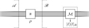
An actual - possibly noisy - measurement (see Fig. 1) acting on a Hilbert space can be described by the following map
| (4) | ||||
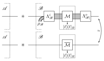
where are the completely positive maps associated to the outcomes . In general, these maps may not be expressed in terms of a single Kraus operator, but as a combination of several ones, i.e. , with . In order to show that a measurement described by acts like a target measurement , it is sufficient to identify a subspace of on which the action of is similar to the one of . Moreover, a map is fully described by its action on one half of a maximally-entangled state, a result known as the Choi-Jamiolkowski isomorphism [37, 38]. Therefore, the equivalence between the considered measurement and the target one is obtained by showing that there exist completely positive trace-preserving maps
| (5) |
and
| (6) | ||||
such that the composition of these maps with the actual measurement is identical to the reference measurement, that is
| (7) |
The injection map and the output map identify subspaces and subsystems in which the measurement acts as the reference measurement see Fig. 2. Note that
the output map does not depend on the measurement output, cf discussion below.
Also note that since all possible outcomes appear in the definition of the maps and – the corresponding Choi states include a description of the labels – equality (7) guarantees at the same time that the outcome states are as expected and that each outcome appears with the desired probability.
Recipe
The aim of this section is to show how the quantity (8) can be lower bounded in the setup presented in Fig. 3. In addition to the source producing the bipartite state and the measurement to be characterised, each party has a measurement box. The box of party has two inputs and while the one of party has four inputs For each measurement input, a binary outcome is obtained called for and for with The measurement can be applied by party before the measurement input is chosen. Although there is no assumption about the Hilbert space dimension and on the proper calibration of the measurement devices, can be characterised in two steps: Step I identifies the quality of the state produced by the source while step II is used to characterise the states after each outcome of the measurement to be certified. The certifications associated to steps I and II are then combined to bound as defined in Eq. (8)
Let us first focus on step I. In this step, the measurement settings and are chosen freely and applied directly on the state produced by the source so that party and can estimate the Clauser, Horne, Shimony, and Holt (CHSH) value [13]
| (9) |
Here, is the expectation value of measurements and . The CHSH value allows one to bound the fidelity of with a maximally-entangled two-qubit state. In particular, the results of Ref. [41] show that there exist local extraction maps and such that
| (10) | ||||
where . Whenever the formula (10) certifies that the source produces up to local maps, these maps being explicitly defined from the quantum description of the measurement inputs and In this case, the same maps can be used to show that ’s settings correspond to the Pauli measurements and while ’s settings correspond to 111Mathematically this means, for example for Bob’s first measurement , that there exists maps and such that Eq. (7) holds with and . Here, can be obtained from through Proposition 4 of [27] (in that work the roles of Alice and Bob are exchanged)..
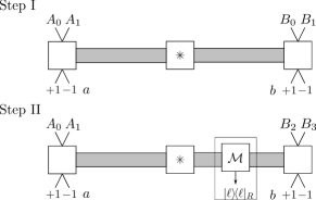
In step II, party applies Let us first consider the state conditioned on the outcome ,
which is characterized using and In particular, parties and are interested in the Bell inequality
| (11) |
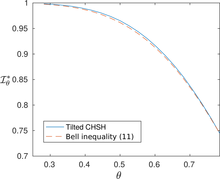
with , whose maximal quantum value is one by construction. We derived this Bell inequality using the variational method presented in [27, 42] to self-test partially-entangled two-qubit pure states in a particularly robust manner. Note that for , Ineq. (11) is the re-normalized CHSH inequality. However, we emphasize that Ineq. (11) is not equivalent to the tilted-CHSH inequality of Refs. [43, 44] but was carefully constructed for the demands of self-testing presented here. The knowledge of allows one to bound the fidelity of the conditional state , that is, to guarantee the existence of local maps and such that
| (12) | |||
Here, is a cutoff parameter corresponding to the violation for which the fidelity matches the square of the largest Schmidt coefficient of . Fig. 4 shows the critical value for both this inequality and the tilted CHSH inequality, as calculated in the Appendix. The previous bound shows that whenever reaches its maximal quantum value the state conditioned on the outcome corresponds to the state up to local maps, these maps being explicitly defined from the quantum description of the measurements performed by and respectively. The same maps can also be used to show that when ’s settings correspond to the Pauli measurements and while ’s inputs correspond to .
The post-measurement state corresponding to the outcome can be characterized with the same measurement boxes and , as well as the same local extraction maps and , see Appendix. Moreover, by including the classical output of the measurement in a global state including a register, as mentioned before, the overall post-measurement state can be written in a compact form
| (13) |
with the post-measurement state associated to outcome , and the probability of this outcome. As the certificates for the two branches and are obtained with the same isometries, they can be combined into a single certificate for . In particular, using the orthogonality of the register states, we have
| (14) |
Taking into account the fact that the fidelity cannot decrease under completely-positive trace-preserving maps and using the triangle inequality we can prove that the fidelity of the state before and after the measurement can be combined to bound the fidelity of the measurement itself, that is,
| (15) |
(see Proposition 5 of [27]). Whenever and for both output states, this bound guarantees that In noisy scenarios, the fidelity that can be certified is shown in Fig. 5.

Note that in case where the fidelity of the state before the measurement cannot be assessed, the quality of the measurement cannot be certified. Indeed, if the source produces the state , and the measurement simply reads out the auxiliary system, then all post-measurement statistics are reproduced. Hence, it is necessary to be able to estimate the quality of the pre-measurement state to give a certificate for the proper functioning of the measurement itself.
Discussion
So far our exposition was focused on the particular example of Kraus operators given by Eq. (1) and (2). Nevertheless, the reader might have noticed that only the tests used to bound the fidelity of the initial state and of the post-measurement states are specific to this example. Consider now a general quantum instrument and assume that one can obtain certificates for the state produced by the source as in Eq. (10) and for all the post-measurement states as in Eq. (12). If the extraction maps on Alice’s side are the same for all certificates, straightforward application of Eqs. (14) and (15) provides a self-testing of the whole instrument. In summary, our approach applies straightforwardly to quantum instruments with an arbitrary number of classical outcomes, including qubit measurements with more than two Kraus operators and measurements on larger-dimensional systems, as well as multipartite instruments.
Note also that we focused on a formulation where the extraction maps in Eq. (6) act trivially on the classical measurement output , that is the extraction maps applied on the quantum output is independent of the measurement result . We believe that this corresponds to the spirit of self-testing in which states and channels are certified up to passive transformations. Nevertheless, a formulation where the extraction maps acting on the post-measurement quantum state depend on the measurement outputs is also possible. In this case it is sufficient to certify the initial and all post-measurement states independently in order to obtain a certificate for the whole instrument. Our derivation then holds as long as Alice’s maps are the same.
Conclusion
We provided a family of Bell inequalities that can be used to self-test non-maximally-entangled two-qubit states with a greater resistance to noise than known Bell inequalities. These results allowed us to derive robust bounds that can be used in practice to certify the quality of qubits measurements beyond the von Neumann model and rank-one POVMs.
This takes essentially three steps. In the first step, the CHSH test is performed without the measurement to evaluate the quantity In the second step, Bell tests are performed after the measurement to be certified is applied on the system, so as to evaluate the values and (see appendix) for each classical output of the instrument. In the third step, the fidelity of the actual measurement is deduced from fidelities of the state before the measurement and of the post-measurement states using the formula given in Eq. (15).
The robustness of our certification techniques together with the flexibility of our recipe make us confident that self-testing of quantum instruments could soon be demonstrated experimentally. For a more theoretical perspective, our results could be naturally extended to self-test only one Kraus operator within a family. This could be obtained by generalizing the ’heralded’ fidelity defined in [26] to the current setting.
References
- [1] B. Hensen, H. Bernien, A. E. Dréau, A. Reiserer, N. Kalb, M. S. Blok, J. Ruitenberg, R. F. L. Vermeulen, R. N. Schouten, C. Abellán, W. Amaya, V. Pruneri, M. W. Mitchell, M. Markham, D. J. Twitchen, D. Elkouss, S. Wehner, T. H. Taminiau, R. Hanson, Loophole-free Bell inequality violation using electron spins separated by 1.3 kilometres, Nature 526, 682 (2015).
- [2] L. K. Shalm, E. Meyer-Scott, B. G. Christensen, P. Bierhorst, M. A. Wayne, M. J. Stevens, T. Gerrits, S. Glancy, D. R. Hamel, M. S. Allman, K. J. Coakley, S. D. Dyer, C. Hodge, A. E. Lita, V. B. Verma, C. Lambrocco, E. Tortorici, A. L. Migdall, Y. Zhang, D. R. Kumor, W. H. Farr, F. Marsili, M. D. Shaw, J. A. Stern, C. Abellán, W. Amaya, V. Pruneri, T. Jennewein, M. W. Mitchell, P. G. Kwiat, J. C. Bienfang, R. P. Mirin, E. Knill, S. W. Nam, Strong Loophole-Free Test of Local Realism, Phys. Rev. Lett. 115, 250402 (2015).
- [3] M. Giustina, M. A. M. Versteegh, S. Wengerowsky, J. Handsteiner, A. Hochrainer, K. Phelan, F. Steinlechner, J. Kofler, J-Å. Larsson, C. Abellán, W. Amaya, V. Pruneri, M. W. Mitchell, J. Beyer, T. Gerrits, A. E. Lita, L. K. Shalm, S. W. Nam, T. Scheidl, R. Ursin, B. Wittmann, A. Zeilinger, Significant-Loophole-Free Test of Bell’s Theorem with Entangled Photons, Phys. Rev. Lett. 115, 250401 (2015).
- [4] W. Rosenfeld, D. Burchardt, R. Garthoff, K. Redeker, N. Ortegel, M. Rau, H. Weinfurter, Event-Ready Bell Test Using Entangled Atoms Simultaneously Closing Detection and Locality Loopholes, Phys. Rev. Lett. 119, 010402 (2017).
- [5] J.S. Bell, On the Einstein Podolsky Rosen paradox, Physics 1, 195 (1964).
- [6] R. Colbeck, Quantum And Relativistic Protocols For Secure Multi-Party Computation, Ph.D. thesis, (2009).
- [7] S. Pironio, A. Acín, S. Massar, A. Boyer de la Giroday, D. N. Matsukevich, P. Maunz, S. Olmschenk, D. Hayes, L. Luo, T. A. Manning, C. Monroe, Random numbers certified by Bell’s theorem, Nature 464, 1021 (2010).
- [8] B. G. Christensen, K. T. McCusker, J. B. Altepeter, B. Calkins, T. Gerrits, A. E. Lita, A. Miller, L. K. Shalm, Y. Zhang, S. W. Nam, N. Brunner, C. C. W. Lim, N. Gisin, and P. G. Kwiat, Detection-Loophole-Free Test of Quantum Nonlocality, and Applications, Phys. Rev. Lett. 111, 130406 (2013).
- [9] Y. Liu, X. Yuan, M-H. Li, W. Zhang, Q. Zhao, J. Zhong, Y. Cao, Y-H. Li, L-K. Chen, H. Li, T. Peng, Y-A. Chen, C-Z. Peng, S-C. Shi, Z. Wang, L. You, X. Ma, J. Fan, Q. Zhang, J-W. Pan, High-Speed Device-Independent Quantum Random Number Generation without a Detection Loophole, Phys. Rev. Lett. 120, 010503 (2018).
- [10] Y. Liu, Q. Zhao, M-H. Li, J-Y. Guan, Y. Zhang, B. Bai, W. Zhang, W-Z. Liu, C. Wu, X. Yuan, H. Li, W. J. Munro, Z. Wang, L. You, J. Zhang, X. Ma, J. Fan, Q. Zhang, J-W. Pan, Device-independent quantum random-number generation, Nature 562, 548 (2018).
- [11] P. Bierhorst, E. Knill, S. Glancy, Y. Zhang, A. Mink, S. Jordan, A. Rommal, Y-K. Liu, B. Christensen, S. W. Nam, M. J. Stevens, L. K. Shalm, Experimentally Generated Randomness Certified by the Impossibility of Superluminal Signals, Nature 556, 223 (2018).
- [12] L. Shen, J. Lee, L. P. Thinh, J-D. Bancal, A. Cerè, A. Lamas-Linares, A. Lita, T. Gerrits, S. W. Nam, V. Scarani, C. Kurtsiefer Randomness Extraction from Bell Violation with Continuous Parametric Down-Conversion, Phys. Rev. Lett. 121, 150402 (2018).
- [13] J. F. Clauser, M. A. Horne, A. Shimony, R.A. Holt, Proposed Experiment to Test Local Hidden-Variable Theories, Phys. Rev. Lett. 23, 880 (1969).
- [14] S. Popescu, D. Rohrlich, Which states violate Bell’s inequality maximally?, Phys. Lett. A 169, 411 (1992).
- [15] M. McKague, T. H. Yang, V. Scarani, Robust self-testing of the singlet, J. Phys. A: Math. Theor. 45, 455304 (2012).
- [16] D. Mayers, A. Yao, Quantum Cryptography with Imperfect Apparatus, Proceedings of the 39th IEEE Conference on Foundations of Computer Science, 1998, page 503, see also Self testing quantum apparatus, Quant. Inf. Comput. 4, 273 (2004).
- [17] M. McKague, Interactive Proofs for BQP via Self-Tested Graph States, Theory of Computing, 12, 3 (2016).
- [18] A. Coladangelo, K.T. Goh, V. Scarani, All Pure Bipartite Entangled States can be Self-Tested, Nat. Comm. 8, 15485 (2017).
- [19] X. Wu, Y. Cai, T. H. Yang, H. Nguyen Le, J-D. Bancal, V. Scarani, Robust self-testing of the three-qubit W state, Phys. Rev. A 90, 042339 (2014).
- [20] J-D. Bancal, M. Navascués, V. Scarani, T. Vértesi, T. H. Yang, Physical characterization of quantum devices from nonlocal correlations, Phys. Rev. A 91, 022115 (2015).
- [21] S-L. Chen, C. Budroni, Y-C. Liang, Y-N. Chen, Natural Framework for Device-Independent Quantification of Quantum Steerability, Measurement Incompatibility, and Self-Testing, Phys. Rev. Lett. 116, 240401 (2016).
- [22] D. Cavalcanti, P. Skrzypczyk, Quantitative relations between measurement incompatibility, quantum steering, and nonlocality, Phys. Rev. A 93, 052112 (2016).
- [23] J. Kaniewski, Self-testing of binary observables based on commutation, Phys. Rev. A 95, 062323 (2017).
- [24] J. Bowles, I. Šupić, D. Cavalcanti, A. Acín, Self-testing of Pauli observables for device-independent entanglement certification, Phys. Rev. A 98, 042336 (2018).
- [25] M-O. Renou, J. Kaniewski, N. Brunner, Self-Testing Entangled Measurements in Quantum Networks, Phys. Rev. Lett. 121, 250507 (2018).
- [26] J-D. Bancal, N. Sangouard, P. Sekatski, Noise-Resistant Device-Independent Certification of Bell State Measurements, Phys. Rev. Lett. 121, 250506 (2018).
- [27] P. Sekatski, J-D. Bancal, S. Wagner, N. Sangouard, Certifying the Building Blocks of Quantum Computers from Bell’s Theorem, Phys. Rev. Lett. 121, 180505 (2018).
- [28] E. S. Gómez, S. Gómez, P. González, G. Cañas, J. F. Barra, A. Delgado, G. B. Xavier, A. Cabello, M. Kleinmann, T. Vértesi, G. Lima, Device-Independent Certification of a Nonprojective Qubit Measurement, Phys. Rev. Lett. 117, 260401 (2016).
- [29] M. Smania, P. Mironowicz, M. Nawareg, M. Pawłowski, A. Cabello, M. Bourennane, Experimental certification of an informationally complete quantum measurement in a device-independent protocol, Optica 7,123-128 (2020).
- [30] E. B. Davies, J. T. Lewis, An operational approach to quantum probability, Comm. Math. Phys. 17, 239 (1970).
- [31] J. A. Gross, C. M. Caves, G. J. Milburn, J. Combes, Qubit models of weak continuous measurements: markovian conditional and open-system dynamics, Quantum Sci. Technol. 3, 024005 (2018).
- [32] R. Silva, N. Gisin, Y. Guryanova, S. Popescu, Multiple Observers Can Share the Nonlocality of Half of an Entangled Pair by Using Optimal Weak Measurements, Phys. Rev. Lett. 114, 250401 (2015).
- [33] F. J. Curchod, M. Johansson, R. Augusiak, M. J. Hoban, P. Wittek, A. Acín Unbounded randomness certification using sequences of measurements, Phys. Rev. A 95, 020102 (2017).
- [34] F. J. Curchod, M. Johansson, R. Augusiak, M. J. Hoban, P. Wittek, A. Acín, A Single Entangled System Is an Unbounded Source of Nonlocal Correlations and of Certified Random Numbers, 12 Conference on the Theory of Quantum Computation, Communication and Cryptography (TQC 2017), Leibniz International Proceedings in Informatics (LIPIcs) 73, 1:1 (2018).
- [35] B. Coyle, M.J. Hoban, E. Kashefi, One-Sided Device-Independent Certification of Unbounded Random Numbers, EPTCS 273, 14 (2018).
- [36] K. Banaszek, I. Devetak, Fidelity trade-off for finite ensembles of identically prepared qubits, Phys. Rev. A 64, 052307 (2001).
- [37] M-D. Choi, Completely positive linear maps on complex matrices, Linear Algebra Appl., 10, 285 (1975).
- [38] A. Jamiołkowski, Linear transformations which preserve trace and positive semidefiniteness of operators, Rep. Math. Phys. 3, 275 (1972).
- [39] M. Raginsky, A fidelity measure for quantum channels, Phys. Lett. A 290, 11 (2001).
- [40] V. P. Belavkin, G. M. D’Ariano, M. Raginsky, Operational distance and fidelity for quantum channels, J. Math. Phys. 46, 062106 (2005).
- [41] J. Kaniewski, Analytic and Nearly Optimal Self-Testing Bounds for the Clauser-Horne-Shimony-Holt and Mermin Inequalities, Phys. Rev. Lett. 117, 070402 (2016).
- [42] P. Sekatski et al., in preparation.
- [43] A. Acín, S. Massar, S. Pironio, Randomness versus Nonlocality and Entanglement, Phys. Rev. Lett, 108, 100402 (2012).
- [44] C. Bamps, S. Pironio, Sum-of-squares decompositions for a family of Clauser-Horne-Shimony-Holt-like inequalities and their application to self-testing, Phys. Rev. A 91, 052111 (2015).
- [45] T. Coopmans, J. Kaniewski, C. Schaffner, Robust self-testing of two-qubit states, Phys. Rev. A 99, 052123 (2019).
Appendix A Appendix
In the supplemental material we will prove the inequality in Eq. (12) of the main text. To do so we have to lower bound the fidelity of an unknown state with respect to
| (16) |
as a function of the expected value of the following Bell expression evaluated on the state
| (17) |
where . Here and in the rest of the appendix we use the short notation and . The Bell expression Eq. (17) has a quantum bound of , achieved by measuring precisely the two-qubit state with the observables
| (18) | ||||||
| (19) |
We find that the local bound of Eq. (17) achieved by the deterministic local strategy is given by
| (20) |
This value is to be compared with the local bound of the well-known (normalized) tilted-CHSH
| (21) |
with , also known to attain the quantum bound of for the partially entangled state of Eq. (16) and well-chosen measurement settings, see Ref. [43, 44] of the main text. We find that the local bound of Eq. (20) is always higher than the local bound of the tilted-CHSH , meaning that the violation of the tilted-CHSH inequality is more robust to white noise than the violation of our new Bell inequality. Nevertheless, our later studies will show that the new Bell operator allows for a more noise-tolerant state certification. The reason for this counter-intuitive result is the following: comparing the observed violation to the local bound only provides information on the distance between the target state (in our case ) and deterministic strategies, given by parallel measurement setting with and product states with and . In self-testing, on the other hand, we need to bound the distance of the target state to arbitrary states for arbitrary measurement settings. It is then crucial that the violation worsens drastically when departing from the perfect settings.
A.1 Fidelity Bounds
To derive lower bounds on the state fidelity from a Bell violation we use the tools presented in Ref. [27] of the main text. There, it is shown that such a global lower bound can be obtained by solving a two-qubit problem. More precisely, the state fidelity can be bounded by minimizing the quantity
| (22) |
with , over all possible two-qubit states and all possible qubit observables (with eigenvalues ) that are compatible with the value of the Bell operator. Here,
| (23) |
are the local extraction channels that can depend on the local observable with for and with for . The first step, therefore, is to fix these extraction channels.
Before we do so, let us fix some notation for the local observables. Any qubit observable with eigenvalues and can be written as with . Furthermore, without loss of generality, we can set the local bases such that
| (24) | ||||
| (25) |
where , . Hence, in the minimization the pairs of observable , and , as well as the extraction channels and only depend on a single parameter and respectively.
A.2 Extraction Channels
The extraction channels we will use are adapted versions of the dephasing channels from Ref. [41] of the main text. Note that since any local map can be seen as an isometry acting on the state plus the auxiliary degrees of freedom, these maps can also be understood as defining local isometries of particular interest. On Alice’s side, the observables are maximally dephased if they are parallel or anti-parallel, and unchanged if they are orthogonal. More precisely, for being half the angle between Alice’s observables in Eq. (24) the dephasing acts according to
| (26) |
where , and if and if . Here and from now on, is the short notation of .
On Bob’s side, the observables are also maximally dephased if they are parallel or anti-parallel, but here they are unchanged if half the angle between them equals , where for the new inequality and for the tilted-CHSH one. For denoting half the angle between Bob’s observables in Eq. (25) the dephasing channel on Bob’s side is
| (27) |
where
| (28) | ||||
| (29) | ||||
| (30) |
For the observables of Bob, the dephasing happens in the direction if and if . Again, we introduced the simplified notation .
Using these extraction channels and applying the numerical method presented Ref. [27] of the main text, we find the values of such that the convex bound
| (31) |
holds for our new inequality, as well as for the tilted-CHSH one (using then instead of ). Here is the observed Bell violation and is the non-trivial cutoff corresponding to the violation for which the fidelity matches the square of the largest Schmidt coefficient of . This means that is the relevant quantity for comparing the self-testing performance of Bell operators in device-independent tasks. Figure 4 in the main text depicts for both the tilted-CHSH and the new inequality.
A.3 Extension to the other state
We have just shown how the observed violation of a Bell inequalities gives a bound on the overlap of the state with the target state
| (32) |
upon applying the extraction maps and . We will now show the violation of another inequality , related to by a mere relabeling of some of the inputs and outputs, bounds the overlap of a state with the other target state
| (33) |
The proof follows the line of Ref. [26] from the main text. Before we start, note that the two target states are related via . In the ideal case this transformation corresponds to a permutation of the outputs of and the exchange of and . We will now show that this observation also holds in the non-ideal case.
Let us first have a closer look at Eq. (31). As it holds for any state , it can be expressed as the expectation value of the operator
| (34) |
where is the Bell operator obtained by choosing the settings (24), (25) in the Bell expression (17). Here we used the fact that the maps are self-adjoint and and . This operator inequality holds for all measurement angles and .
Now consider a new Bell expression corresponding to an operator , obtained by exchanging the outputs of and exchanging the role of the measurements and in the previous expression. The operator can be obtained by applying the rotation :
| (35) |
as illustrated in Figure 6.
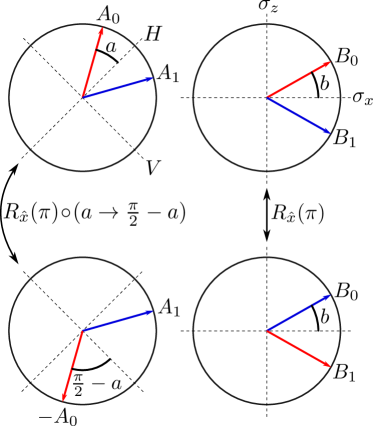
Since Eq. (34) holds for all angles, it also holds for . Then we act with and from the left and right respectively. We arrive at
| (36) | ||||
The rotation on Bob’s side commutes with the extraction channel . This is easily verified by reminding ourselves that and therefore .
On Alice’s side, we realize that . Therefore . By also recalling that , we find that .
Combining everything and using , Eq. (36) is equivalent to
| (37) |
which implies that with the same extraction channels and observables, and a new Bell test , one can device-independently self-test the second output state .
