Global symmetry (0-symmetry) acts on the whole space while higher $k$-symmetry acts on all the codimension-$k$ closed subspaces. The usual condensed matter lattice theories do not include dynamical electromagnetic (EM) field and do not have higher symmetries (unless we engineer fine-tuned toy models). However, for gapped systems, (anomalous) higher symmetries can emerge from the usual condensed matter theories at low energies (usually in a spontaneously broken form). We pointed out that the emergent spontaneously broken higher symmetries are nothing but a kind of topological orders. Thus the study of emergent spontaneously broken higher symmetries is a study of topological order. The emergent (anomalous) higher symmetries can be used to constrain possible phase transitions and possible phases induced by certain types of excitations in topological orders. (Anomalous) higher symmetry can also emerge in gapless systems if the gapless excitations contain gapless gauge fields. In particular, EM condensed matter systems that include the dynamical EM field have an emergent anomalous $U(1)$-1-symmetry below the energy gap of the magnetic monopoles. So EM condensed matter systems can realize some physical phenomena of anomalous higher symmetry. In particular, any gapped liquid phase of an EM condensed matter system (induced by arbitrary fluctuations and condensations of electric charges and photons) must have a non-trivial bosonic topological order.

Emergent (anomalous) higher symmetries from topological orders
and from dynamical electromagnetic field in condensed matter systems

I Introduction

A global symmetry acts on the whole space, and a local symmetry acts on all the points (i.e. all the sub manifolds of 0-dimension). A higher symmetry, such as a $k$-symmetry, acts on all the closed sub manifolds of codimension $k$. Thus a global symmetry is a 0-symmetry. A lattice Hamiltonian system has a $k$-symmetry, if the Hamiltonian is invariant under certain unitary transformations defined on all the closed codimension-$k$ subspaces.

Higher symmetry had been studied before in lattice systems, where exactly soluble lattice Hamiltonians commuting with closed string and/or closed membrane operators were constructedKitaev (2003); Wen (2003a); Levin and Wen (2003); Yoshida (2011); Bombín (2014) to realize topological ordersWen (1989); Wen and Niu (1990); Wen (1990). A direct relation between higher symmetries and topological orders was pointed out in LABEL:NOc0605316,NOc0702377, under the name low-dimensional gauge-like symmetries.

The term higher form symmetry was first introduced in LABEL:GW14125148, where it was stressed that higher symmetry can be viewed as a generalization of the global symmetry (i.e. 0-symmetry) and many results and intuitions for global symmetry can be extended to higher symmetry. For a Lagrangian field theory in $(d+1)$-dimensional spacetime, a 0-symmetry is generated by constant fields (closed $0$-forms) in spacetime, such as $\varphi\to\varphi+c$, while a $k$-symmetry is generated by closed $k$-forms in spacetime. From the field theory definition of the $k$-symmetry generated by a closed $k$-form $\alpha_{k}$, it appears that we require the field theory to have a $k$-form field $a_{k}$ so that the $k$-symmetry transformation can be written as $a_{k}\to a_{k}+\alpha_{k}$. However, from the lattice point of view, a $k$-symmetry does not require a $k$-form field.

The emergence of higher symmetry from lattice model without higher symmetry was also studied before in 2005Hastings and Wen (2005), under the name of emergent gauge symmetry. A topological robustness of emergent higher symmetry against any local perturbation was discovered. Such a topological robustness was used to show the topological robustness of a Goldstone-like theorem for spontaneous broken continuous higher symmetry: the gapless $U(1)$ gauge bosons from spontaneous breaking of $U(1)$ higher symmetry remain to be gapless even after we explicitly break the higher symmetry by arbitrary perturbations. The result of LABEL:HW0541 also suggests that every topological order containing Abelian gauge theory has emergent higher symmetry.

Recently, higher symmetry and higher anomaly, as well as the related higher symmetry protected trivial (SPT) orders and higher gauge theories, became an active topic in field theory.Baez and Schreiber (2007); Girelli et al. (2008); Baez and Huerta (2011); Kapustin and Thorngren (2013); Gaiotto et al. (2015); Sharpe (2015); Thorngren and von Keyserlingk (2015); Bullivant et al. (2017a); Costa de Almeida et al. (2017); Tachikawa (2017); Parzygnat (2018); Delcamp and Tiwari (2018); Lake (2018); Cordova et al. (2018); Hofman and Iqbal (2019); Bouzid and Tahiri (2018); Benini et al. (2018); Nikolaus and Waldorf (2018); Zhu et al. (2018); Harlow and Ooguri (2018); Wan and Wang (2018a, b); Guo et al. (2018); Wan and Wang (2018c) LABEL:TK151102929,BM170200868,KR180505367 discussed higher symmetry and higher anomaly in lattice systems. LABEL:TK151102929 studied higher SPT phases and higher anomaly in-flow. LABEL:BM170200868 discussed how to construct a lattice Hamiltonian of a higher gauge theory. LABEL:KR180505367 obtained a Lieb-Schultz-Mattis type theorem from higher anomalies.

In this paper, we will concentrate on applications of higher symmetry to condensed matter systems, by studying the lattice aspect of higher symmetry, higher anomaly, and how higher symmetry in field theory can emerge from lattice models without higher symmetry. The following is a summary of the results:

1. The usual condensed matter theories (which do not include the dynamical electromagnetic field) do not have higher symmetries. However, higher symmetries can emerge in usual gapped condensed matter theories in a spontaneously broken form, at energies below the energy gap. In fact, the spontaneously broken finite higher symmetry is nothing but a special kind of topological orders (see Section IV).

2. If certain topological excitations in topological orders have very large energy gap $\Delta_{\text{top}}$, while other topological excitations have small gaps of order $\Delta\ll\Delta_{\text{top}}$, we may have emergent higher symmetry or emergent anomalous higher symmetry at energies below $\Delta_{\text{top}}$. Note that such an emergent (anomalous) higher symmetry can appear at energies above $\Delta$, and is smaller than the emergent higher symmetry below $\Delta$. Thus emergent (anomalous) higher symmetry in a topological order is characterized by a set ${\cal C}_{\text{a}}$ of low energy allowed topological excitations. The set is closed under the fusion and braiding of the topological excitations (see Section IV).

3. For bosonic 2+1D Abelian topological orders, the emergent higher symmetry characterized by ${\cal C}_{\text{a}}$ is anomaly free iff the topological excitations in ${\cal C}_{\text{t}}$ are bosons with trivial mutual statistics. Here ${\cal C}_{\text{t}}$ is the set of topological excitations that have trivial mutual statistics with all the topological excitations in ${\cal C}_{\text{a}}$ (see Section IV).

4. The emergent (anomalous) higher symmetry will constrain the possible phase transitions and phases induced by the low energy topological excitations (see Section VI). In particular, for a topological order with emergent anomalous higher symmetry characterized by ${\cal C}_{\text{a}}$, the topological order cannot change into a trivial phase with no topological order no matter how we condense the topological excitations in ${\cal C}_{\text{a}}$.

5. Anomalous higher symmetries can be realized at boundary of higher symmetry protected topological states in one higher dimension protected by the corresponding anomaly-free higher symmetry.

6. We find a spacetime lattice regularization of 3+1D $U^{\kappa}(1)$ gauge theory with $2\pi$-quantized topological term

   $$\ \ \ Z=\int D[a_{I}] \hskip 1.0pt\mathrm{e}^{\hskip 1.0pt\mathrm{i}\hskip 1.0pt\int_{M^{4}}\frac{K_{IJ}}{4\pi}f_{I}f_{J}-\int_{M^{4}}\frac{|f_{I}|^{2}}{g}},$$ (1)

   where $f_{I}=\hskip 1.0pt\mathrm{d}a_{I}$ is the field-strength 2-form of the $U(1)$ gauge field $a_{I}$. We show that the lattice model is a local bosonic model with a $Z_{k_{1}}\times Z_{k_{2}}\times\cdots$-1-symmetry which is determined by the even integer matrix $K$, where $k_{I}$ are the diagonal elements of the Smith normal form of $K$. The lattice model (VI.4) is exactly soluble on closed spacetime in $g\to\infty$ limit, and realizes a higher SPT phase (see Section VI.4).

7. The Abelian higher symmetry and the non-Abelian 0-symmetry can have a non-trivial mix described by a higher group.Kapustin and Thorngren (2013); Cordova et al. (2018) In this paper, we discuss a general way to construct lattice models with a combined 0-symmetry, 1-symmetry, etc (see Section VIII).

8. We systematically construct lattice bosonic models that realize higher SPT phases with higher symmetry described by higher group ${\cal B}(G,\Pi_{2},\cdots)$ in any dimension.Thorngren and von Keyserlingk (2015) Our construction suggests a (many-to-one) classification of $(d+1)$D bosonic higher SPT phases in terms of the cohomology of an extended higher group: $H^{d+1}[{\cal B}(G\leftthreetimes SO_{\infty},\Pi_{2},\cdots),\mathbb{R}/\mathbb{Z}]$ (see Section IX.3). Using fermion worldline decoration, we also systematically construct lattice fermionic models that realize higher SPT phases with higher symmetry ${\cal B}(G_{f},\Pi_{2},\cdots)$ in any dimension (see Section IX.4).

9. The condensed matter theories that include the dynamical electromagnetic (EM) field (which will be called the EM condensed matter theories) can be viewed as local bosonic theories with an anomalous $U(1)$-1-symmetry, since the magnetic monopoles can be ignored at low energies. Such an anomaly comes from the property that all fermions carry odd electric charges and all bosons carry even electric charges. Using the anomalous $U(1)$-1-symmetry, we show that any gapped liquid phaseZeng and Wen (2015); Swingle and McGreevy (2016) of any EM condensed matter system must have a non-trivial bosonic topological order (see Section XI).

Exactly soluble models have been constructed to realize various topological orders Kitaev (2003); Wen (2003a); Levin and Wen (2003); Yoshida (2011); Bombín (2014). The toy model Hamiltonian commute with closed string and/or membrane operators, and thus has higher symmetries. However, the real condensed matter systems (after ignoring the dynamical electromagnetic field) do not have higher symmetries. In this paper we pointed out the topologically ordered phases and the states near the topologically ordered phases has emergent higher symmetries bellow the energy gap of some topological excitations. Thus if those topological excitations remain to be gapped, we can use the emergent higher symmetries to study the low energy dynamics and phase transition of the topologically ordered phases.

II Notations and conventions

In part of this paper, we will use extensively the notion of cochain, cocycle, and coboundary, as well as their higher cup product $\underset{{\scriptscriptstyle k}}{\smile}$ and Steenrod square $\mathbb{Sq}^{k}$. A brief introduction can be found in Appendix A. We will abbreviate the cup product $a\smile b$ as $ab$ by dropping $\smile$. We will use $\overset{\scriptscriptstyle n}{=}$ to mean equal up to a multiple of $n$, and use $\overset{\scriptscriptstyle\hskip 1.0pt\mathrm{d}}{=}$ to mean equal up to $\hskip 1.0pt\mathrm{d}f$ (i.e. up to a coboundary). We will use $\langle l,m\rangle$ to denote the greatest common divisor of $l$ and $m$ ($\langle 0,m\rangle\equiv m$). We will also use $\lfloor x\rceil$ to denote the integer that is closest to $x$. (If two integers have the same distance to $x$, we will choose the smaller one, eg $\lfloor\frac{1}{2}\rceil=0$.)

In this paper, we will deal with many $\mathbb{Z}_{n}$-value quantities. We will denote them as, for example, $a^{\mathbb{Z}_{n}}$. However, we will always lift the $\mathbb{Z}_{n}$-value to $\mathbb{Z}$-value, so the value of $a^{\mathbb{Z}_{n}}$ has a range from $-\lfloor\frac{N}{2}\rceil$ to $\lfloor\frac{N}{2}\rceil$. In this case, even the expression like $a^{\mathbb{Z}_{n}}+a^{\mathbb{Z}_{m}}$ makes sense.

We introduced a symbol $\leftthreetimes$ to construct fiber bundle $X$ from the fiber $F$ and the base space $B$:

$$pt\to F\to X=F\leftthreetimes B\to B\to pt.$$ (2)

We will also use $\leftthreetimes$ to construct group extension of $H$ by $N$ Morandi (1997):

$$1\to N\to N\leftthreetimes_{e_{2},\alpha}H\to H\to 1.$$ (3)

Here $e_{2}\in H^{2}[H;Z(N)]$, $Z(N)$ is the center of $N$, and $\alpha:H\to\text{Aut}(N)$ is a non-trivial action of $H$ on $Z(N)$. Thus $e_{2}$ and $\alpha$ characterize different group extensions.

We will use $K(\Pi_{1},\Pi_{2},\cdots,\Pi_{n})$ to denote a connected topological space with homotopy group $\pi_{i}(K(\Pi_{1},\Pi_{2},\cdots,\Pi_{n}))=\Pi_{i}$ for $1\leq i\leq n$, and $\pi_{i}(K(\Pi_{1},\Pi_{2},\cdots,\Pi_{n}))=0$ for $i>n$. If only one of the homotopy groups, say $\Pi_{d}$, is non-trivial, then $K(\Pi_{1},\Pi_{2},\cdots,\Pi_{n})$ is the Eilenberg-MacLane space, which is denoted as $K(\Pi_{d},d)$. If only two of the homotopy groups, say $\Pi_{d}$, $\Pi_{d^{\prime}}$, is non-trivial, then we denote the space as $K(\Pi_{d},d;\Pi_{d^{\prime}},d^{\prime})$, etc. We will use ${\cal B}(\Pi_{1};\Pi_{2};\cdots;\Pi_{n})$, ${\cal B}(\Pi_{d},d)$, and ${\cal B}(\Pi_{d},d;\Pi_{d^{\prime}},d^{\prime})$ to denote the simplicial sets with only one vertex satisfying Kan conditions that describe a special triangulation of $K(\Pi_{1},\Pi_{2},\cdots,\Pi_{n})$, $K(\Pi_{d},d)$, and $K(\Pi_{d},d;\Pi_{d^{\prime}},d^{\prime})$ respectively. Since simplicial sets satisfying Kan conditions are viewed as higher groupoids in higher category theory, the simplicial sets ${\cal B}(\Pi_{1};\Pi_{2};\cdots;\Pi_{n})$, ${\cal B}(\Pi_{d},d)$, and ${\cal B}(\Pi_{d},d;\Pi_{d^{\prime}},d^{\prime})$, with only one vertex (unit), can be viewed as higher groups. In this paper, higher groups are treated therefore as this sort of special simplicial sets, as in LABEL:ZW180809394.

III Symmetry and higher symmetry on lattice

The notion of phase and phase transition play a major role in condensed matter physics in our attempts to understand properties of various materials. However, to mathematically define the concepts of quantum phase and quantum phase transition at zero temperature, we need to first introduce the notion Hamiltonian class. The notions of phase and phase transition can only be defined relative to a Hamiltonian class. (For example, the notion of phase is not a property of a single Hamiltonian.)

For example, we can define a Hamiltonian class as a set of local Hamiltonians for bosons on lattice. Relative to such a Hamiltonian class, we can define the notion bosonic topological orders.Wen (1989); Wen and Niu (1990) Such a precise definition of bosonic topological orders allows us to classify them in 1 spatial dimensionFannes et al. (1992); Verstraete et al. (2005) where there is no non-trivial bosonic topological orders, as well as in 2 spatial dimensionsWen (1990); Kitaev (2006); Rowell et al. (2009); Wen (2015a); Lan et al. (2016) and in 3 spatial dimensionsLan et al. (2018); Lan and Wen (2019), where very rich bosonic topological orders exist.

We may define another Hamiltonian class as a set of local Hamiltonians for fermions on lattice. Relative to such a Hamiltonian class, we can define the notion fermionic topological orders.Gu et al. (2015) There is only one non-trivial fermionic topological order in 1 spatial dimension – the 1+1D topological $p$-wave superconductor.Kitaev (2001); Levitov et al. (2001) The fermionic topological orders in 2 spatial dimensions are classified in LABEL:LW150704673, and a proposal to classify fermionic topological orders in 3 spatial dimensions is given in LABEL:LW180108530.

We can also introduce a Hamiltonian class as a set of local Hamiltonians $H$ on lattice with an on-site symmetryChen et al. (2013); Wen (2013) described by a group $G$:

$$HW_{g}=W_{g}H,\ \ \ W_{g}=\prod_{i}W_{g}(i),\ \ \ g\in G,$$ (4)

where $W_{g}(i)$ is a representation of the symmetry group $G$ acting on the local Hilbert space on site-$i$. Relative to such a Hamiltonian class, we can define the notion of spontaneous symmetry breaking orders, symmetry protected topological (SPT) ordersGu and Wen (2009); Chen et al. (2011a) (also known as symmetry protected trivial ordersWen (2015b, 2017a)), and symmetry enriched topological (SET) orders.Chen et al. (2010); Lu and Vishwanath (2013); Chang et al. (2015); Ye (2018) The classification of spontaneous symmetry breaking orders is given by a pair of groups $G_{\text{grnd}}\subset G$, where $G_{\text{grnd}}$ is the symmetry group of the ground state (the unbroken symmetry group). The classification of SPT and SET orders are given in LABEL:CGW1107,SPC1139,CGL1314,CY14126589,LW160205946,LW170404221,LW180108530,KT170108264,WG170310937,WG181100536, via group cohomology theory, cobordism theory, and (higher) category theory.

The on-site symmetry $G$ is also called global symmetry. However, a global symmetry in field theory or in lattice theory may not be an on-site symmetry $G$. In this case, we sayWen (2013); Kapustin and Thorngren (2014) the global symmetry to have a t’ Hooft anomaly.’t Hooft (1980) We will also call the on-site symmetry $G$ as an on-site 0-symmetry, where the symmetry transformation acts on codimension-0 space or spacetime.Gaiotto et al. (2015); Lake (2018)

Now, we are ready to define higher symmetry on lattice, by introducing a Hamiltonian class as a set of local Hamiltonians $H$ on a triangulation of $d$-dimensional space (which is a more precise definition of lattice) that satisfy

$$HW_{a}(C^{d-k})=W_{a}(C^{d-k})H,$$ (5)

for any $d-k$-dimensional (i.e. codimension-$k$) closed subcomplex $C^{d-k}$ of the triangulated $d$-dimensional space. Here $W_{a}(C^{d-k})$ is an operator that acts on the degrees of freedom on the closed subcomplex $C^{d_{k}}$ with the following “on-site” property

$$W_{a}=\prod_{i\in C^{d-k}}W_{a}(i).$$ (6)

The operator $W_{a}(C^{d-k})$ labeled by $a$ satisfy a so called pointed fusion rule

$$W_{a}(C^{d-k})W_{b}(C^{d-k})=W_{c}(C^{d-k}),$$ (7)

and they commute with each other

$$[W_{a}(C^{d-k}),W_{b}(\tilde{C}^{d-k})]=0.$$ (8)

Such a pointed fusion rule makes the index set $\{a\}$ into an Abelain group $\Pi$. The Hamiltonian class defined above is referred as having an on-site $k$-symmetry since the symmetry acts on codimension-$k$ subcomplex of the space.Gaiotto et al. (2015); Lake (2018)

IV An example of anomaly-free (on-site) $Z_{2}$-1-symmetry

IV.1 The 3+1D bosonic lattice model

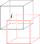
Figure 1: ( Color online) A cubic lattice (black) and its dual cubic lattice (red). The index $\bm{i}$ labels the faces of the cubic lattice and the links of the dual cubic lattice.

The simplest on-site 1-symmetry is a $Z_{2}$-1-symmetry. Let us consider a qubit model on a 3-dimensional cubic lattice (see Fig. 1), where the qubits live on the square faces of the cubic lattice. We choose the closed subcomplex $C^{2}$ to the closed 2-dimensional surfaces formed by the square faces of the cubic lattice. The generator of the $Z_{2}$-1-symmetry is given by

$$W(C^{2})=\prod_{\bm{i}\in C^{2}}\sigma^{z}_{\bm{i}}$$ (9)

where $\bm{i}$ labels the square faces of the cubic lattice. We can check that $W(C^{2})$’s all commute with each other and their pointed fusion is described by a $Z_{2}$ group. So we say $W(C^{2})$ generates an on-site $Z_{2}$ 1-symmetry.

A Hamiltonian with the above $Z_{2}$ 1-symmetry is given byKitaev (2003); Wen (2003a); Levin and Wen (2003)

$$H =-U_{1}\sum_{\langle\bm{i}\bm{j}\bm{k}\bm{l}\rangle}\sigma^{x}_{\bm{i}}\sigma^{x}_{\bm{j}}\sigma^{x}_{\bm{k}}\sigma^{x}_{\bm{l}}$$ (10)

$$\ \ \ \ -U_{2}\sum_{\langle\bm{i}\bm{j}\bm{k}\bm{l}\bm{m}\bm{n}\rangle}\sigma^{z}_{\bm{i}}\sigma^{z}_{\bm{j}}\sigma^{z}_{\bm{k}}\sigma^{z}_{\bm{l}}\sigma^{z}_{\bm{m}}\sigma^{z}_{\bm{n}}-B\sum_{\langle\bm{i}\rangle}\sigma^{z}_{\bm{i}},$$

where $\sum_{\langle\bm{i}\rangle}$ sums over all the square faces, $\sum_{\langle\bm{i}\bm{j}\bm{k}\bm{L}\bm{m}\bm{n}\rangle}$ sums over all cubes, and $\sum_{\langle\bm{i}\bm{j}\bm{k}\bm{l}\rangle}$ sums over all squares formed by the links in the dual cubic lattice. (We note that $\bm{I}$’s also label the links of the dual cubic lattice. See Fig. 1)

When $|B|\ll|U_{1}|,|U_{2}|$, the Hamiltonian (10) has a topologically ordered ground state. The topological order is described by a $Z_{2}$ gauge theory. A pair of $Z_{2}$-charge $e$ is created by an open string operator

$$S_{\text{str}}(\tilde{C}^{1})=\prod_{\bm{i}\in\text{ string }\tilde{C}^{1}}\sigma^{x}_{\bm{i}},$$ (11)

where the string is formed by the links of the dual cubic lattice. Note that the open string creation operators break the $Z_{2}$-1-symmetry. Thus we cannot even include the short open string operators in the Hamiltonian. This implies that in the presence of the $Z_{2}$-1-symmetry, the $Z_{2}$-charge is not mobile. A $Z_{2}$-flux loop $s$ is created by an open membrane operator bounded by the loop:

$$M_{\text{memb}}(C^{2})=\prod_{\bm{i}\in\text{ membrane }C^{2}}\sigma^{z}_{\bm{i}},$$ (12)

where the membrane is formed by the square faces of the original cubic lattice. The $Z_{2}$-1-symmetry allow the Hamiltonian to have such a open membrane operator. Thus the $Z_{2}$-flux loop $s$ is mobile even in the presence of the $Z_{2}$-1-symmetry.

We also note that the closed membrane operator happen to be the generator (9) of the $Z_{2}$-1-symmetry. Thus we say that the $Z_{2}$-1-symmetry is generated by the topological excitations of the $Z_{2}$-flux loops.

IV.2 $Z_{2}$-1-symmetry and unbreakable strings

In this subsection, we discuss a meaning of 1-symmetry in our lattice model eqn. (10). Let $|\uparrow\rangle$, $|\downarrow\rangle$ be the eigenstates of $\sigma^{z}$. We view $\otimes_{\bm{i}}|\uparrow\rangle_{\bm{i}}$ as a reference state. We create a closed-string state by changing $|\uparrow\rangle_{\bm{i}}$ to $|\downarrow\rangle_{\bm{i}}$ for $\bm{i}$ on closed strings. Here strings are formed by links of the dual cubic lattice.

Because of the $Z_{2}$-1-symmetry, the ground state of eqn. (10) is a superposition of closed strings (assuming $U_{2},B>0$). When $B=0$, the ground state is an equal weight superposition of all closed strings, and spontaneously break the $Z_{2}$-1-symmetry (on space with non-trivial first homotopy group $\pi_{1}$). When $B\to+\infty$, the ground state has no strings and does not break the $Z_{2}$-1-symmetry.

From this example, we see that the physical meaning of the $Z_{2}$-1-symmetry is the appearance of unbreakable strings. Even when we force a string breaking, the $Z_{2}$-1-symmetry requires that the end of the string (i.e. the $Z_{2}$-charge) cannot move and have no dynamics.

To summarize, the $Z_{2}$-1-symmetry is generated by the $Z_{2}$-flux-line excitations. Such a $Z_{2}$-1-symmetry forbid the excitations that have non-trivial mutual statistics with the $Z_{2}$-flux lines, such as the $Z_{2}$-charge excitations. This can be achieved by including the $Z_{2}$-1-symmetry generator (9) in the Hamiltonian with a large coefficient (the $U_{2}$ term in eqn. (10)), which gives the $Z_{2}$-charge a large energy gap.

IV.3 Emergence of generic higher symmetry in topological orders

The above physical understanding of $Z_{2}$-1-symmetry can also be generalized:

If a topological order contains a topological excitation $\eta$ of unit quantum dimension, then the topological order can have an emergent higher symmetry generated by $\eta$ below an energy gap $\Lambda$, if all the topological excitations with non-trivial mutual statistics respect to any combination of $\eta$ have a large gap beyond $\Lambda$.

We note that the emergent higher symmetry allows the topological excitations with trivial mutual statistics respect to $\eta$ to have a small gap, or even become gapless and drive a phase transition via their condensation. The emergent higher symmetry will be present through the phase transition.

To understand the above result in more details, let us consider a dimension-$n$ topological excitation in a topological order. We assume that the topological excitation can be created by a dimension-$n+1$ operator $W_{1}(C^{n+1})$ at its boundary $\partial C^{n+1}$. Here $W_{1}(C^{n+1})$ is a operator acts on the $(n+1)$-dimensional subcomplex $C^{n+1}$ in the space (not spacetime). If the quantum dimension of the topological excitation is 1, then $W_{1}(C^{n+1})$ on a closed subcomplex $C^{n+1}$ generates a $Z_{N}$ fusion

$$W_{a}(C^{n+1})W_{b}(C^{n+1})=W_{a+b}(C^{n+1}),\ \ \ W_{N}(C^{n+1})=1,$$ (13)

for a certain integer $N$. Now, we require the lattice Hamiltonians to commute with $W_{1}(C^{n+1})$ for all closed $C^{n+1}$. This way we obtain a Hamiltonian system that has a $Z_{n}$ $D-n-2$-symmetry where $D$ is the spacetime dimension. If a Hamiltonian with such a higher symmetry realizes the above topological order, then all the topological excitations with non-trivial mutual statistics with the $n$-dimensional topological excitation are not mobile. We can even make those topological excitations to have a large gap by adding the $W_{a}(C^{n+1})$ terms to the Hamiltonian with a large coefficient. Only topological excitations having trivial mutual statistics with the $n$-dimensional topological excitation are allowed to appear at low energies and to have non-trivial dynamics.

We stress that, in our construction, the higher symmetry is a property of the pair: the topological order plus the allowed low energy topological excitations: the higher symmetry is generated from the topological excitations of unit quantum dimension that have trivial mutual statistics with the allowed low energy topological excitations. Even in the same topological order, allowing different types of topological excitations to appear at low energy will leads to different (anomalous) higher symmetries. Later, we will present several examples of this phenomenon.

For the 3+1D $Z_{2}$ topological order discussed above, if we only allow the $Z_{2}$-flux line excitations at low energies (i.e. the $Z_{2}$-charges associated with the string ends all have very high energies), then we will have the $Z_{2}$ 1-symmetry at low energies, generated by the $Z_{2}$-flux lines. Later we will show that if we only have the $Z_{2}$-charge excitations at low energies, we will have a $Z_{2}$-2-symmetry at low energies (see eqn. (62)), generated by the $Z_{2}$-charge excitations. If we only allow the trivial excitations at low energies, then we will have the $Z_{2}$-1-symmetry generated by the $Z_{2}$-flux lines, and the $Z_{2}$-2-symmetry, generated by the $Z_{2}$-charge excitations. If we allow both $Z_{2}$-flux and $Z_{2}$-charge excitations at low energies, we will explicitly break the $Z_{2}$-1-symmetry and the $Z_{2}$-2-symmetry at low energies. In fact, there are no topological excitations that have trivial mutual statistics with both $Z_{2}$-flux and $Z_{2}$-charge excitations, and there is no higher symmetry.

We like to remark that the above $Z_{2}$-1-symmetry and $Z_{2}$-2-symmetry have mixed anomaly between them (see Section LABEL:). A system with both of those higher symmetries cannot realize a trivial topological order.

IV.4 Generalized higher symmetry

In the above, we have constructed a higher symmetry from one topological excitation of unit quantum dimension. Certainly, we can construct more general higher symmetry from several topological excitations of unit quantum dimension. We can even construct something from a topological excitations with higher quantum dimensions. We call the “something” generalized higher symmetry (see LABEL:KLTW):

A topological order can have an emergent generalized higher symmetry generated by a topological excitation $\eta$, if all the topological excitations with non-trivial mutual statistics respect to any combination of $\eta$ have a large gap.

Since a topological order, by definition, always has a finite energy gap, at energies much below the energy gap, the topological order always has an emergent generalized higher symmetry, and such a generalized higher symmetry is spontaneously broken. If the topological order contains excitations with unit quantum dimension, then, part of the generalized higher symmetry can be viewed as the higher symmetry. If certain topological excitations have a large gap and other topological excitations have a small gap, then below the large gap, the topological order may have an emergent generalized higher symmetry, which may be smaller then the emergent generalized higher symmetry below the small gap.

IV.5 Spontaneous higher symmetry breaking and topological order

When $|B|\gg|U_{1}|,|U_{2}|$, the ground state of the Hamiltonian (10) is a product state without topological order. When $|B|\ll|U_{1}|,|U_{2}|$, the ground state has a non-trivial topological order. The small $|B|$ topologically ordered phase and the large $|B|$ trivial phase can also be distinguished by spontaneous 1-symmetry breaking. The $Z_{2}$-1-symmetry is generated by $W(C^{2})$ in eqn. (9).

On space $S^{1}\times S^{1}\times S^{1}$, the large $|B|$ trivial phase has an unique ground state, which is is invariant under all the $Z_{2}$-1-symmetry transformations. The $Z_{2}$-1-symmetry is not broken. While the topologically ordered phase for small $|B|$ has 8 ground states on space $S^{1}\times S^{1}\times S^{1}$. Some the $Z_{2}$-1-symmetry transformations act non-trivially in the 8-dimensional ground state subspace, i.e. are not propotional to an identity operator. Thus, the $Z_{2}$-1-symmetry is spontaneously broken.

The spontaneous 1-symmetry broken state is nothing but a topologically ordered state. Since the 1-symmetry is not spontaneously broken in the large $|B|$ trivial product state, the transition from the trivial product state to the topologically ordered state can be viewed as a spontaneous breaking of the 1-symmetry. This result is general:

A spontaneous higher symmetry broken state always corresponds to a topologically ordered state.

Here we have assumed that the higher symmetry is finite. The spontaneous breaking of continuous higher symmetry is discussed in LABEL:GW14125148,L180207747, and give rise to gapless states. However, even though the spontaneous breaking of continuous higher symmetry produce gapless excitations, the gaplessness of the excitations do not need higher symmetry. Even after we explicitly break the higher symmetry, the gapless excitations remain gapless (see Section VII).Hastings and Wen (2005) This is very different from the gapless excitations from the spontaneous breaking of continuous 0-symmetry.

We also like to point out that a topologically ordered state can be more general and may not correspond to a spontaneous higher symmetry broken state. For example, we can break the higher symmetry explicitly. Even without higher symmetry, we can still have topologically order. Even though, some topological orders, such as $Z_{2}$-gauge theory, can be viewed as spontaneous higher symmetry broken states. Some other topological orders, such as $S_{3}$-gauge theory, cannot be viewed as spontaneous higher symmetry broken states, since spontaneous 1-symmetry broken states only give rise to Abelian gauge theory.

IV.6 The usefulness of higher symmetry in condensed matter

We see that some topological orders can be understood as spontaneous higher symmetry breaking in the systems with higher symmetry. But the usual condensed matter theories on lattice never have higher symmetry. (Here by “usual condensed matter theories” we mean the theories that do not include the dynamical electromagnetic fields.) So it appears that this way to understand topological order may not be very useful. Also, this way to understand topological order misses a key feature of topological order: topological order is robust against any local perturbation that can break all the symmetries and higher symmetries.

However, the notion of higher symmetry and their spontaneous breaking can still be useful in condensed matter in the following sense: A gapped liquid stateZeng and Wen (2015); Swingle and McGreevy (2016) may have many emergent symmetries and higher symmetries at low energies. If some of the emergent higher symmetries are spontaneously broken, then the corresponding gapped liquid state has topological orders. This allows us to use spontaneously broken emergent higher symmetry to characterize a subclass of topological orders.

The higher symmetries in low energy effective field theory may come from lattice model with exact higher symmetry, or may emerge from a lattice model that has no higher symmetry. Therefore, even though the usual condensed matter theories on lattice do not have higher symmetry, low energy effective theories with higher symmetries can still be used to describe condensed matter systems, since higher symmetry can be emergent.

Later, we will see that if we include the dynamical electromagnetic (EM) fields in condensed matter theories, the resulting EM condensed matter theories will have an approximate $U(1)$-1-symmetry if we ignore the magnetic monopoles. (The appearance of magnetic monopoles in condensed matter energy scale will break the $U(1)$ higher symmetry.) In this sense, $U(1)$-1-symmetry is useful for real condensed matter systems.

The notion of higher symmetry can also be useful for condensed matter in another way. We can construct toy models with higher symmetries, and make the ground states spontaneous break the higher symmetry. This way, we construct toy models that realize some topological orders. There are already many different ways to construct exactly soluble models to systematically realize topological orders, SPT orders, and SET orders.Kitaev (2003); Levin and Wen (2005); Gu et al. (2015); Walker and Wang (2012); Chen et al. (2013); Bhardwaj et al. (2017); Williamson and Wang (2017); Zhu et al. (2018); Wang and Gu (2018) But it does not hurt to have one more construction. In this paper, we will construct some simple toy models with higher symmetry that realize some topological orders, SET orders, and SPT orders.

Last, higher symmetry can also be used to constrain possible phase transitions and possible phases.Kobayashi et al. (2018) In certain topological orders, if we only allow a certain type of topological excitations at low energies, the topological orders plus the topological excitations may have an emergent (anomalous) higher symmetry. Then any phase transition induced by this particular type of topological excitations must preserve the anomaly of the higher symmetry. This puts constraint on possible phase transitions and possible resulting phases.

V An example of anomalous $Z_{2}$-1-symmetry

V.1 The 2+1D bosonic lattice model

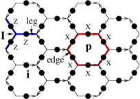
Figure 2: ( Color online) A qubit model, where qubits live on the links of a honeycomb lattice. $\bm{I}$ labels the vertices and $\bm{i}$ labels the links (the qubits) of the honeycomb lattice.

In this section, we are going discuss another simple lattice that have several $Z_{2}$-1-symmetries and one of them is an anomalous $Z_{2}$-1-symmetry. In this model the qubits live on the links of a honeycomb lattice (see Fig. 2), with a Hamiltonian:Kitaev (2003)

$$H =-U\sum_{\bm{I}}Q_{\bm{I}}-g\sum_{\bm{p}}F_{\bm{p}},$$

$$Q_{\bm{I}} =\prod_{\text{legs of }\bm{I}}\sigma^{z}_{\bm{i}},$$

$$F_{\bm{p}} =\prod_{\text{edges of }\bm{p}}\sigma^{x}_{\bm{i}},$$ (14)

where $\sum_{\bm{I}}$ sum over the vertices and where $\sum_{\bm{p}}$ sum over the hexagons of the honeycomb lattice (see Fig. 2). Notice that $H$ is a sum of commuting operators $[F_{\bm{p}},F_{\bm{p}^{\prime}}]=0$, $[Q_{\bm{I}},Q_{\bm{I}^{\prime}}]=0$, $[F_{\bm{p}},Q_{\bm{I}}]=0$, and $F_{\bm{p}}^{2}=Q_{\bm{I}}^{2}=1$ Thus the ground state $|\Psi_{\text{grnd}}\rangle$ is given by $F_{\bm{p}}|\Psi_{\text{grnd}}\rangle=Q_{\bm{I}}|\Psi_{\text{grnd}}\rangle=|\Psi_{\text{grnd}}\rangle$

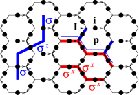
Figure 3: ( Color online) The string operators.

There are two types of topological excitations above the ground state with $Q_{\bm{I}}=F_{\bm{p}}=1$: $e$-type with $Q_{\bm{I}}=-1$ and $m$-type with $F_{\bm{p}}=-1$. Those excitations cannot be created individually. They can only be created in pairs by string operators.

We have type-$e$ string operator $W_{e}(C_{1})=\prod_{\bm{i}\in C_{1}}\sigma^{x}_{\bm{i}}$ where the string $C_{1}$ is formed by the links of the honeycomb lattice (see Fig. 3). An open $e$-string operator creates two $e$-type topological excitations at its ends. We also have type-$m$ string operator $W_{m}(\tilde{C}_{1})=\prod_{\bm{i}\in\tilde{C}_{1}}\sigma^{z}_{\bm{i}}$ where the string $\tilde{C}_{1}$ is formed by the links of dual of the honeycomb lattice (see Fig. 3). An open $m$-string operator creates two $m$-type topological excitations at its ends.

We can also fuse the $e$-string and $m$-string operators together to form a type-$f$ string operator $W_{f}(C_{1}\prod\tilde{C}_{1})=\prod_{\bm{i}\in_{1}C_{1}}\sigma^{x}_{\bm{i}}\prod_{\bm{i}\in\tilde{C}_{1}}\sigma^{z}_{\bm{i}}$ where the string $C_{1}$ in the lattice and the string $\tilde{C}_{1}$ in the dual lattice closely follow each other (see Fig. 3). An open $f$-string operator creates two $f$-type topological excitations at its ends. It turns out that $e$ and $m$ are bosons, and $f$ is a fermion. They all have a $\pi$ mutual statistics respect to each other.

We find that $H$ in eqn. (V.1) commutes with the above three types of string operators if the strings are closed:

$$[H,W^{\text{closed}}_{e}]=[H,W^{\text{closed}}_{m}]=[H,W^{\text{closed}}_{f}]=0.$$ (15)

Therefore, our lattice model has two $Z_{2}$-1-symmetries since

$$W_{e}^{2}=W_{m}^{2}=W_{f}^{2}=1,\ \ \ W_{e}W_{m}=W_{f}.$$ (16)

On a torus, the model (V.1) has four degenerate ground states, and the closed string operators $W^{\text{closed}}_{e}$, $W^{\text{closed}}_{m}$, and $W^{\text{closed}}_{f}$ act non-tivially in the ground state subspace when the closed strings are not contractible. Thus the ground state on eqn. (V.1) spontaneously breaks the two $Z_{2}$-1-symmetries, and has a $Z_{2}$ topological order.

Now we consider the following model with $U\gg g,J$

$$H =-U\sum_{\bm{I}}Q_{\bm{I}}-g\sum_{\bm{p}}F_{\bm{p}}-J\sum_{\bm{i}}\sigma^{z}_{\bm{i}},$$

$$Q_{\bm{I}} =\prod_{\bm{i}\in\bm{I}}\sigma^{z}_{\bm{i}},\ \ \ F_{\bm{p}}=\prod_{\bm{i}\in\bm{p}}\sigma^{x}_{\bm{i}}$$ (17)

As we go from $g\gg J$ to $g\ll J$ the ground state undergoes a phase transition that change the $Z_{2}$ topological order to trivial product state, driven by $m$ particle condensation. This is because that the $J$-term is the hopping for $m$ and can drive the $m$ excitations to have a negative energy.

The above Hamiltonian and the transition has the $Z_{2}^{m}$-1-symmetry generated by the closed $m$-strings $W_{m}(\tilde{C}_{1})=\prod_{\bm{i}\in\tilde{C}_{1}}\sigma^{z}_{\bm{i}}$, but does not have the $Z_{2}^{e}$-1-symmetry generated by the closed $e$-strings $W_{e}(C_{1})=\prod_{\bm{i}\in C_{1}}\sigma^{x}_{\bm{i}}$ and the $Z_{2}^{f}$-1-symmetry generated by the closed $f$-strings $W_{f}(C_{1}\prod\tilde{C}_{1})$.

The end of $W_{m}$ (the 1-symmetry generator) is the $m$ particle. The low energy allowed excitations of the above Hamiltoniam are the particles with trivial mutual statistics with the $m$ particle. Thus the low energy allowed excitations include the $m$ particles, but not include the $e$ particles and the $f$ particles (the fermions).

To summerize, the $Z_{2}$ topological order in 2+1D has three type of topological excitations:
1. the $Z_{2}$-charge $e$ – boson
2. the $Z_{2}$-flux $m$ – boson
3. the charge-flux bound state $f=m\otimes e$ – fermion
The three particles have mutual $\pi$ statistics respect to each other. Below the minimal gap of the three particles $\Delta_{e},\Delta_{m},\Delta_{f}$, we have three $Z_{2}$-1-symmetries generated by closed string operators $W_{e}(C_{1})$, $W_{m}(\tilde{C}_{1})$, and $W_{f}(C_{1}\otimes\tilde{C}_{1})$.

If $\Delta_{m}\ll\Delta_{e},\Delta_{f}$, then below $\Delta_{e},\Delta_{f}$ (but may be above $\Delta_{m}$), we have a $Z_{2}$-1-symmetry generated by closed string operators $W_{m}(\tilde{C}_{1})$, but not the ones from $W_{e}(C_{1})$ and $W_{f}(C_{1}\otimes\tilde{C}_{1})$. The low energy allowed particles are ${\cal C}_{a}=\{m\}$. The 1-symmetry is generated by string operators for the particles ${\cal C}_{\text{t}}=\{m\}$. If we reduce $\Delta_{m}$ to make it negative, we will induce a Bose-condensation of the $Z_{2}$-flux and a $Z_{2}^{m}$-1-symmetric confinement transition: the $Z_{2}$ topological order is changed the trivial product state.

If $\Delta_{f}\ll\Delta_{e},\Delta_{m}$, then below $\Delta_{e},\Delta_{m}$ (but may be above $\Delta_{f}$), we have a $Z_{2}$-1-symmetry generated by closed string operators $W_{f}(C_{1}\otimes\tilde{C}_{1})$, but not the ones from $W_{e}(C_{1})$ and $W_{m}(\tilde{C}_{1})$. The low energy allowed particles is ${\cal C}_{a}=\{f\}$, and the 1-symmetry is generated by string operators for the particles ${\cal C}_{\text{t}}=\{f\}$.

If we reduce $\Delta_{f}$ to make it negative, can we still induce confinement transition to change the $Z_{2}$ topological order to a trivial product state with no topological order? Since $f$ is a fermion, it cannot Bose-condense. But it can condense into some other topologically ordered state. Can the new topological order cancel the parent $Z_{2}$ topological order to produce a trivial phase without topological order?

The condensation of $f$ is a $Z_{2}^{f}$-1-symmetric phase transition. We will show later that the $Z_{2}^{f}$-1-symmetry is anomalous, and the $Z_{2}^{f}$-1-symmetric phase transition cannot induce a trivial product state.

V.2 On-site/non-on-site higher symmetry

To understand the anomalous higher symmetry, let us first review the connection between non-on-site symmetry and anomalous symmetry.Wen (2013) An on-site symmetry (on-site 0-symmetry) of group $G$ is generated by a transformation of the following form:

$$U(g)=\prod_{i}U_{i}(g),\ \ \ U(g)U(h)=\prod_{i}U_{i}(gh)=U(gh),$$ (18)

where $g,h\in G$, $i$ label the lattice site and $U_{i}(g)$ only acts on the degrees of freedom on site-$i$. The on-site symmetry can be gauged to get a local $G^{\otimes N_{\text{site}}}$ symmetry

$$U(\{g_{i}\}) =\prod_{i}U_{i}(g_{i}),$$

$$U(\{g_{i}\})U(\{h_{i}\}) =\prod_{i}U_{i}(g_{i}h_{i})=U(\{g_{i}h_{i}\}).$$ (19)

An on-site symmetry is also called anomaly-free symmetry.

Roughly speaking, an non-on-site symmetry of group $G$ does have the product form

$$U(g)\neq[\prod_{i}U_{i}(g)],\ \ \ \ U(g)U(h)=U(gh).$$ (20)

It cannot be gauged to get a $G^{\otimes N_{\text{site}}}$ symmetry:

$$U(\{g_{i}\}) =\prod_{i}U_{i,i+1}(g_{i}),$$

$$U(\{g_{i}\})U(\{h_{i}\}) \neq U(\{g_{i}h_{i}\}).$$ (21)

An non-on-site symmetry is also called anomalous symmetry. For a more accurate discussion of non-on-site and anomalous symmetry, see LABEL:W1313.

Similarly, an on-site $k$-symmetry of an Abelian group $\Pi$ in $d$-dimensional space is given by

$$U(C_{d-k},g) =\prod_{i\in C_{d-k}}U_{i}(g),$$

$$U(g)U(h) =\prod_{i\in C_{d-k}}U_{i}(gh)=U(gh),\ g\in\Pi_{2}.$$ (22)

Here we stress that we have assumed that the space is a complex (a lattice) and there are independent degrees of freedom living on the $(d-k)$-cells of the complex. The operator $U_{i}(g)$ only acts on the degrees of freedom on the $(d-k)$-cell labeled by $i$. $C_{d-k}$ is a collection of $(d-k)$-cells and $\prod_{i\in C_{d-k}}$ is a product over all the $(d-k)$-cells in $C_{d-k}$.

The on-site $(d-1)$-symmetry can be gauged

$$U(C_{d-k},\{g_{i}\})=\prod_{i\in C_{d-k}}U_{i}(g_{i}),$$ (23)

$$U(C_{d-k},\{g_{i}\})U(C_{d-k},\{h_{i}\})=U(C_{d-k},\{g_{i}h_{i}\}).$$

An on-site higher symmetry is also called anomaly-free higher symmetry.

Non-on-site $(d-1)$-symmetry for a group $\Pi$

$$U(C_{d-k},g)\neq\prod_{i\in C_{d-k}}U_{i}(g),$$

$$U(C_{d-k},g)U(C_{d-k},h)=U(C_{d-k},gh),\ \ \ \ g\in\Pi.$$ (24)

The non-on-site higher symmetry cannot be gauged

$$U(C_{d-k},\{g_{i}\})U(C_{d-k},\{h_{i}\})\neq U(C_{d-k},\{g_{i}h_{i}\}).$$ (25)

A non-on-site higher symmetry is called anomalous higher symmetry, if we cannot make it on-site via some local unitary operations.Chen et al. (2010) More precisely

A higher symmetry (which may be generated by operators in several different dimensions) is anomaly-free if it allows a symmetric ground state with trivial topological order. A higher symmetry is anomalous if it does not allow a symmetric ground state with trivial topological order.

For example, the $Z_{2}$-1-symmetry generated by $W_{e}(C_{1})=\prod_{i\in C_{1}}\sigma^{x}_{i}$ are on-site and anomaly-free. We note that the open string operator $W_{e}(C_{1})$ creates two bosons at its ends.

Also, the $Z_{2}$-1-symmetry generated by $W_{m}(\tilde{C}_{1})=\prod_{j\in\tilde{C}_{1}}\sigma^{z}_{j}$ are on-site and anomaly-free. Again the open string operator $W_{m}(\tilde{C}_{1})$ creates two bosons at its ends.

The $Z_{2}$-1-symmetry generated by $W_{f}(C_{1}\otimes\tilde{C}_{1})=\prod_{i\in C_{1}}\sigma^{x}_{i}\prod_{j\in\tilde{C}_{1}}\sigma^{z}_{j}$ is not on-site and maybe anomalous. But how to determine if a higher symmetry is anomaly-free or anomalous? Later, we will show that an 1-symmetry generated by a string operator $W(C_{1})$ is anomaly-free if and only if the end of the string is a boson. So the $Z_{2}$-1-symmetry generated by $W_{f}(C_{1}\otimes\tilde{C}_{1})=\prod_{i\in C_{1}}\sigma^{x}_{i}\prod_{j\in\tilde{C}_{1}}\sigma^{z}_{j}$ is anomalous, since the end of string $W_{f}(C_{1}\otimes\tilde{C}_{1})$ is a fermion. In fact, one can show that the open string operators $W_{f}(C_{1}\otimes\tilde{C}_{1})$ satisfy the so-called fermion-hopping algebra, which make the string end to be a fermion. The string operators satisfying fermion-hopping algebra cannot be made into on-site operators.

The $Z_{2}\times Z_{2}$-1-symmetry generated by $W_{e}(C_{1})=\prod_{i\in C_{1}}\sigma^{x}_{i}$ and by $W_{m}(\tilde{C}_{1})=\otimes_{j\in\tilde{C}_{1}}\sigma^{z}_{j}$ is also anomalous. This is because it contains the $Z_{2}$-1-symmetry generated by $W_{f}(C_{1}\otimes\tilde{C}_{1})=\prod_{i\in C_{1}}\sigma^{x}_{i}\prod_{j\in\tilde{C}_{1}}\sigma^{z}_{j}$ which is anomalous. We also note that the end of string $W_{e}(C_{1})$ and the end of string $W_{m}(\tilde{C}_{1})$ have a non-trivial mutual statistics between them, which implies a mixed anomaly between the two $Z_{2}$-1-symmetries.

If we have a higher symmetry of generated by operators in several dimensions defined on the same spacial complex, $U(C_{d-k_{1}},g_{1})$, $U(C_{d-k_{2}},g_{2})$, $\cdots$ and if all those operators are on-site, then the higher symmetry a anomaly-free. We note that since all the operators are defined on the same spacial complex the higher symmetry generators with different dimensions act on different degrees of freedoms living on cells of different dimensions. So the higher symmetry generators with different dimensions always commute with each other. If some higher symmetry generators are defined on a complex while other higher symmetry generators are defined on the dual complex, then the higher symmetry generators may not commute and may be anomalous.

Table 1: The higher category theory is actually a theory of pointlike, stringlike, $\cdots$, excitations in physics.Kong and Wen (2014) This table lists the corresponding concepts in mathematics and in physics.

Concepts in higher category	Concepts in physics
Unitary $D$-category ${\cal M}$	Topological excitations with their braiding fusion properties in a topologically ordered state in $D$-spacetime dimension
Objects (0-morphisms)	The ground states
Simple 1-morphisms	The codimension-1 topological excitations
Simple $D-2$-morphisms	The stringlike topological excitations
Simple $D-1$-morphisms	The pointlike topological excitations
Composite morphisms	The topological excitations with accidental degeneracy
The collection of simple $D-1$-morphisms, simple $D-2$-morphisms, etc	Topological excitations
Trivial morphisms	The excitations that can be created by local operators (non-topological excitations)

More generally, the boundary of higher symmetry generators can produce pointlike, stringlike, $\cdots$, topological excitations. We can use a higher category ${\cal C}_{\text{t}}$ with one object to describe their fusion and braiding (see Table 1). In fact the higher category ${\cal C}_{\text{t}}$ characterizes the higher symmetry completely. We like to conjecture that

The higher symmetry is anomaly-free if and only if all the morphisms in ${\cal C}_{\text{t}}$ have a unit quantum dimension, and have no phase factor under exchange, braiding and fusion.

Here the statement “have no phase factor under exchange, braiding and fusion” need a more precise definition. For pointlike excitations in 2-dimensional space and higher, “no phase factor under exchange and braiding” means that the pointlike excitations are all bosons with trivial mutual statistics. If the fusion of some excitations is described by a pointed fusion category, the “no phase factor under fusion” means the $F$-symbol of the fusion category is equal to 1. For more details, see LABEL:KLTW.

VI Simple lattice examples that realize higher symmetry protected topological phases

One way to show a higher symmetry in a system is anomalous is to show that the symmetric system can be regarded as a boundary of higher symmetry protected topological (hSPT) state in one-higher dimension, using the relation between anomaly and SPT state in one-higher dimension.Wen (2013) In this section, we will describe some examples of hSPT states. Using those examples, we will show that a higher symmetry generated by several types of closed string operator is anomaly-free only if the ends of string are bosons with trivial mutual statistics with each others.

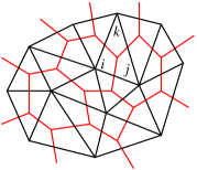
Figure 4: (Color online) The black lines describe a 2-dimensional spacetime complex ${\cal M}^{2}$. The red lines describe the dual complex $\tilde{{\cal M}}^{2}$.

To construct lattice models with 0-symmetries and higher symmetries, it is more convenient to do so in the spacetime Lagrangian formalism. We construct a spacetime lattice by first triangulating a $D$-dimensional spacetime manifold $M^{D}$. (In this paper, we will use $D$ to denote spacetime dimensions and $d$ to denote space dimensions.) So a spacetime lattice is a $D$-complex ${\cal M}^{D}$ with vertices labeled by $i$, links labeled by $ij$, triangles labeled by $ijk$, etc(see Fig. 4). The $D$-complex ${\cal M}^{D}$ also has a dual complex denoted as $\tilde{{\cal M}}^{D}$. The vertices of ${\cal M}^{D}$ correspond to the $D$-cells in $\tilde{{\cal M}}^{D}$, The links of ${\cal M}^{D}$ correspond to the $(D-1)$-cells in $\tilde{{\cal M}}^{D}$, etc

Our spacetime lattice model may have a field living on the vertices, $g_{i}$. Such a field is called a 0-cochain. The model may also have a field living on the links, $a_{ij}$. Such a field is called a 1-cochain, etc. To construct spacetime lattice models, in particular, the topological spacetime lattice models,Kapustin and Thorngren (2013); Thorngren and von Keyserlingk (2015); Wen (2017b); Lan et al. (2018) we will use extensively the mathematical formalism of cochains, coboundaries, and cocycles (see Appendix A). The relation between the spacetime path integral approach and the Hamiltonian approach is discussed in Appendix B.

VI.1 A 3+1D model to realize a pure $Z_{n}$-1-SPT phase

VI.1.1 The bulk theory and the boundary theory

In this section, we will consider a 3+1D bosonic model on a spacetime complex ${\cal M}^{4}$, with $\mathbb{Z}_{n}$-valued dynamic field $a^{\mathbb{Z}_{n}}_{ij}$ on the links $ij$ of the complex ${\cal M}^{4}$. We also have a $\mathbb{Z}_{n}$-valued non-dynamical background field $\hat{B}^{\mathbb{Z}_{n}}_{ijk}$ on the triangles $ijk$ of the complex ${\cal M}^{4}$. The path integral of our bosonic model is given by

$$Z =\sum_{\{a^{\mathbb{Z}_{n}}\}}\hskip 1.0pt\mathrm{e}^{2\pi\hskip 1.0pt\mathrm{i}\hskip 1.0pt\int_{{\cal M}^{4}}\frac{k}{n}\mathbb{Sq}^{2}(\hat{B}^{\mathbb{Z}_{n}}+\hskip 1.0pt\mathrm{d}a^{\mathbb{Z}_{n}})},$$ (26)

$$(k,n)=(\text{integer},\text{integer}),$$

where $\sum_{\{a^{\mathbb{Z}_{n}}\}}$ sums over $\mathbb{Z}_{n}$-valued 1-cochains $a^{\mathbb{Z}_{n}}$, and $\hat{B}^{\mathbb{Z}_{n}}$ is a $\mathbb{Z}_{n}$-valued 2-cocycle

$$\hskip 1.0pt\mathrm{d}\hat{B}^{\mathbb{Z}_{n}}\overset{\scriptscriptstyle n}{=}0.$$ (27)

Also $\mathbb{Sq}^{2}$ is the generalized Steenrod square defined by eqn. (202). We will show that the above model realizes a $Z_{n}$-1-SPT phase.

Since $\hat{B}^{\mathbb{Z}_{n}}$ and $a^{\mathbb{Z}_{n}}$ are $\mathbb{Z}_{n}$-valued, we require the action amplitude $\hskip 1.0pt\mathrm{e}^{2\pi\hskip 1.0pt\mathrm{i}\hskip 1.0pt\int_{{\cal M}^{4}}\frac{k}{n}(\hat{B}^{\mathbb{Z}_{n}}+\hskip 1.0pt\mathrm{d}a^{\mathbb{Z}_{n}})^{2}}$ to be invariant under the transformation

$$\hat{B}^{\mathbb{Z}_{n}}\to\hat{B}^{\mathbb{Z}_{n}}+nb^{\mathbb{Z}},\ \ \ \ a^{\mathbb{Z}_{n}}\to a^{\mathbb{Z}_{n}}+nu^{\mathbb{Z}},$$ (28)

where $b^{\mathbb{Z}}$ and $u^{\mathbb{Z}}$ are any $\mathbb{Z}$ valued 2-cochain and 1-cochain. (To do the addition $a^{\mathbb{Z}_{n}}+nu^{\mathbb{Z}}$, we have lifted the $\mathbb{Z}_{n}$-value of $a^{\mathbb{Z}_{n}}$ to $\mathbb{Z}$.) From eqn. (A), we see that

$$\ \ \ \ \mathbb{Sq}^{2}(nb^{\mathbb{Z}}+\hat{B}^{\mathbb{Z}_{n}})=n^{2}\mathbb{Sq}^{2}(b^{\mathbb{Z}})+\mathbb{Sq}^{2}(\hat{B}^{\mathbb{Z}_{n}})+2nb^{\mathbb{Z}}\hat{B}^{\mathbb{Z}_{n}}$$

$$+n\hskip 1.0pt\mathrm{d}\hat{B}^{\mathbb{Z}_{n}}\underset{{\scriptscriptstyle 2}}{\smile}\hskip 1.0pt\mathrm{d}b^{\mathbb{Z}}-n\hskip 1.0pt\mathrm{d}(\hat{B}^{\mathbb{Z}_{n}}\underset{{\scriptscriptstyle 1}}{\smile}b^{\mathbb{Z}})-n\hskip 1.0pt\mathrm{d}(\hskip 1.0pt\mathrm{d}\hat{B}^{\mathbb{Z}_{n}}\underset{{\scriptscriptstyle 2}}{\smile}b^{\mathbb{Z}})$$

$$\overset{\scriptscriptstyle n}{=}\mathbb{Sq}^{2}(\hat{B}^{\mathbb{Z}_{n}}).$$ (29)

We see that the action amplitude $\hskip 1.0pt\mathrm{e}^{2\pi\hskip 1.0pt\mathrm{i}\hskip 1.0pt\int_{{\cal M}^{4}}\frac{k}{n}(\hat{B}^{\mathbb{Z}_{n}}+\hskip 1.0pt\mathrm{d}a^{\mathbb{Z}_{n}})^{2}}$ is indeed invariant under eqn. (28) even when ${\cal M}^{4}$ has a boundary. The above result implies that the model has a $Z_{n}$-1-symmetry generated by

$$a^{\mathbb{Z}_{n}}\to a^{\mathbb{Z}_{n}}+\alpha^{\mathbb{Z}_{n}},\ \ \ \hskip 1.0pt\mathrm{d}\alpha^{\mathbb{Z}_{n}}\overset{\scriptscriptstyle n}{=}0,$$ (30)

even when ${\cal M}^{4}$ has a boundary.

In eqn. (26), $\hat{B}^{\mathbb{Z}_{n}}$ is the $\mathbb{Z}_{n}$ background 2-connection to describe the twist of the $Z_{n}$-1-symmetry. The model has a $Z_{n}$ gauge symmetry:

$$a^{\mathbb{Z}_{n}}\to a^{\mathbb{Z}_{n}}+\hat{a}^{\mathbb{Z}_{n}},\ \ \ \ \ \hat{B}^{\mathbb{Z}_{n}}\to\hat{B}^{\mathbb{Z}_{n}}-\hskip 1.0pt\mathrm{d}\hat{a}^{\mathbb{Z}_{n}}.$$ (31)

Using eqn. (207) we find that

$$\ \ \ \ \mathbb{Sq}^{2}(\hat{B}^{\mathbb{Z}_{n}}+\hskip 1.0pt\mathrm{d}a^{\mathbb{Z}_{n}})$$ (32)

$$=\mathbb{Sq}^{2}\hat{B}^{\mathbb{Z}_{n}}+2\hat{B}^{\mathbb{Z}_{n}}\hskip 1.0pt\mathrm{d}\hat{a}^{\mathbb{Z}_{n}}+\hskip 1.0pt\mathrm{d}[\mathbb{Sq}^{2}\hat{a}^{\mathbb{Z}_{n}}-\hskip 1.0pt\mathrm{d}\hat{a}^{\mathbb{Z}_{n}}\underset{{\scriptscriptstyle 1}}{\smile}\hat{B}^{\mathbb{Z}_{n}}]$$

$$\overset{\scriptscriptstyle 2n}{=}\mathbb{Sq}^{2}\hat{B}^{\mathbb{Z}_{n}}+\hskip 1.0pt\mathrm{d}[\hat{a}^{\mathbb{Z}_{n}}\hskip 1.0pt\mathrm{d}\hat{a}^{\mathbb{Z}_{n}}-\hskip 1.0pt\mathrm{d}\hat{a}^{\mathbb{Z}_{n}}\underset{{\scriptscriptstyle 1}}{\smile}\hat{B}^{\mathbb{Z}_{n}}+\hat{B}^{\mathbb{Z}_{n}}\hat{a}^{\mathbb{Z}_{n}}]$$

Therefore

$$\hskip 1.0pt\mathrm{e}^{2\pi\hskip 1.0pt\mathrm{i}\hskip 1.0pt\int_{{\cal M}^{4}}\frac{k}{n}\mathbb{Sq}^{2}(\hat{B}^{\mathbb{Z}_{n}}+\hskip 1.0pt\mathrm{d}a^{\mathbb{Z}_{n}})}=\hskip 1.0pt\mathrm{e}^{2\pi\hskip 1.0pt\mathrm{i}\hskip 1.0pt\int_{{\cal M}^{4}}\frac{k}{n}\mathbb{Sq}^{2}(\hat{B}^{\mathbb{Z}_{n}})}$$ (33)

for closed spacetime ${\cal M}^{4}$. The model is exactly soluble and gapped for closed spacetime ${\cal M}^{4}$.

Eqn. (26) has no topological order since on closed spacetime and for $\hat{B}^{\mathbb{Z}_{n}}=0$

$$Z =\sum_{\{a^{\mathbb{Z}_{n}}\}}\hskip 1.0pt\mathrm{e}^{2\pi\hskip 1.0pt\mathrm{i}\hskip 1.0pt\int_{{\cal M}^{4}}\frac{k}{n}(\hskip 1.0pt\mathrm{d}a^{\mathbb{Z}_{n}})^{2}}=\sum_{\{a^{\mathbb{Z}_{n}}\}}1=n^{N_{l}},$$ (34)

where $N_{l}$ is the number of links in the spacetime complex ${\cal M}^{4}$. $n^{N_{l}}$ is the so called the volume term that is linear in the spacetime volume. The topological partition function $Z^{\text{top}}$ is given via

$$Z=\hskip 1.0pt\mathrm{e}^{-\epsilon V}Z^{\text{top}}$$ (35)

where $V$ is the spacetime volume. (For a detailed discussion of the non-universal volume term and the universal topological terms, see LABEL:KW1458,WW180109938.) After removing the volume term, the topological partition function of the above model is $Z^{\text{top}}({\cal M}^{4})=1$ for all closed 4-complex ${\cal M}^{4}$. Thus the above model has no topological order. After we turn on the flat $Z_{n}$ 2-connection $\hat{B}^{\mathbb{Z}_{n}}$, the topological partition function of the model (26) is

$$Z^{\text{top}}({\cal M}^{4},\hat{B}^{\mathbb{Z}_{n}})=\hskip 1.0pt\mathrm{e}^{2\pi\hskip 1.0pt\mathrm{i}\hskip 1.0pt\int_{{\cal M}^{4}}\frac{k}{n}(\hat{B}^{\mathbb{Z}_{n}})^{2}},\ \ \ \hskip 1.0pt\mathrm{d}\hat{B}^{\mathbb{Z}_{n}}\overset{\scriptscriptstyle n}{=}0.$$ (36)

The above 1-SPT invariant looks different for different $k$ mod $n$. But are they really different? If we gauge the $Z_{n}$-1-symmetry, we turn the above $Z_{n}$-1-SPT phase into a topological ordered phase described by a pure $Z_{n}$ 2-gauge theory:Zhu et al. (2018)

$$Z =\sum_{\{\hskip 1.0pt\mathrm{d}b^{\mathbb{Z}_{n}}\overset{\scriptscriptstyle n}{=}0\}}\hskip 1.0pt\mathrm{e}^{2\pi\hskip 1.0pt\mathrm{i}\hskip 1.0pt\int_{{\cal M}^{4}}\frac{k}{n}(\hat{b}^{\mathbb{Z}_{n}})^{2}}.$$ (37)

It turns out that the same topological order is also described by a $Z_{\langle 2k,n\rangle}$ gauge theory. The $Z_{\langle 2k,n\rangle}$ gauge theory has emergent fermions iff $2kn/\langle 2k,n\rangle^{2}=\text{odd}$. So the 1-SPT invariant is really different at least when the pairs $[\langle 2k,n\rangle,\text{mod}(2kn/\langle 2k,n\rangle^{2},2)]$ are different.

In LABEL:ZW180809394, it was shown that $H^{4}({\cal B}(Z_{n},2);\mathbb{R}/\mathbb{Z})=\mathbb{Z}_{n}$ for $n=\text{odd}$, and $H^{4}({\cal B}(Z_{n},2);\mathbb{R}/\mathbb{Z})=\mathbb{Z}_{2n}$ for $n=\text{even}$. Thus the above 1-SPT invariant is non-tirivial. There are (at least) $n$ distinct $Z_{n}$-1-SPT phases labeled by $k=0,\cdots,n-1$.

To see the physical properties of the $Z_{n}$-1-SPT phase, we consider its 2+1D boundary state described by

$$Z({\cal B}^{3}) =\sum_{\{a^{\mathbb{Z}_{n}}\}}\hskip 1.0pt\mathrm{e}^{2\pi\hskip 1.0pt\mathrm{i}\hskip 1.0pt\int_{{\cal B}^{3}}\frac{k}{n}a^{\mathbb{Z}_{n}}\hskip 1.0pt\mathrm{d}a^{\mathbb{Z}_{n}}}$$ (38)

where we have set the background 2-connection $\hat{B}^{\mathbb{Z}_{n}}=0$. The boundary theory also has the $Z_{n}$-1-symmetry which is generated by eqn. (30). We like to point out that the action amplitude $\hskip 1.0pt\mathrm{e}^{2\pi\hskip 1.0pt\mathrm{i}\hskip 1.0pt\int_{{\cal B}^{3}}\frac{k}{n}a^{\mathbb{Z}_{n}}\hskip 1.0pt\mathrm{d}a^{\mathbb{Z}_{n}}}$ for spacetime with boundary $\partial{\cal B}^{3}\neq 0$ is actually not invariant under the $Z_{n}$-1-symmetry transformation. Only the action amplitude for closed spacetime $\partial{\cal B}^{3}=0$ has the $Z_{n}$-1-symmetry. This indecates that the $Z_{n}$-1-symmetry in the 2+1D model eqn. (38) is anomalous.

The 2+1D model is not exactly soluble. To have a soluble model, we restrict $a^{\mathbb{Z}_{n}}$ to be cocycles and obtain

$$Z({\cal B}^{3}) =\hskip-13.00005pt\sum_{\{\hskip 1.0pt\mathrm{d}a^{\mathbb{Z}_{n}}\overset{\scriptscriptstyle n}{=}0\}}\hskip-13.00005pt\hskip 1.0pt\mathrm{e}^{2\pi\hskip 1.0pt\mathrm{i}\hskip 1.0pt\int_{{\cal B}^{3}}\frac{k}{n}a^{\mathbb{Z}_{n}}\hskip 1.0pt\mathrm{d}a^{\mathbb{Z}_{n}}}=\sum_{\{\hskip 1.0pt\mathrm{d}a^{\mathbb{Z}_{n}}\overset{\scriptscriptstyle n}{=}0\}}1.$$ (39)

The above model actually describes a 2+1D untwisted $Z_{n}$ gauge theory.

In the presence of the $Z_{n}$-flux described by 2-coboundary $\hskip 1.0pt\mathrm{d}\hat{a}^{\mathbb{Z}_{n}}$ and the $Z_{n}$ charge described by worldline $C^{1}$, the above path integral is modified. The new one is obtained by adding the term $\hskip 1.0pt\mathrm{e}^{\frac{2\pi}{n}\hskip 1.0pt\mathrm{i}\hskip 1.0pt\int_{C^{1}}a^{\mathbb{Z}_{n}}}$ and then replacing $a^{\mathbb{Z}_{n}}$ by $a^{\mathbb{Z}_{n}}+\hat{a}^{\mathbb{Z}_{n}}$. We find

$$Z({\cal B}^{3}) =\hskip-15.00002pt\sum_{\{\hskip 1.0pt\mathrm{d}a^{\mathbb{Z}_{n}}\overset{\scriptscriptstyle n}{=}0\}}\hskip-13.00005pt\hskip 1.0pt\mathrm{e}^{2k\pi\hskip 1.0pt\mathrm{i}\hskip 1.0pt\int_{{\cal B}^{3}}a^{\mathbb{Z}_{n}}\beta_{n}a^{\mathbb{Z}_{n}}+\frac{2k\pi}{n}\hskip 1.0pt\mathrm{i}\hskip 1.0pt\int_{{\cal B}^{3}}(2a^{\mathbb{Z}_{n}}\hskip 1.0pt\mathrm{d}\hat{a}^{\mathbb{Z}_{n}}+\hat{a}^{\mathbb{Z}_{n}}\hskip 1.0pt\mathrm{d}\hat{a}^{\mathbb{Z}_{n}})}$$

$$\ \ \ \ \ \ \ \ \hskip 1.0pt\mathrm{e}^{\frac{2\pi}{n}\hskip 1.0pt\mathrm{i}\hskip 1.0pt\int_{C^{1}}(a^{\mathbb{Z}_{n}}+\hat{a}^{\mathbb{Z}_{n}})}.$$ (40)

Let $\tilde{c}_{2}$ be the Poincaré dual of the cycle $C^{1}$ which is a 2-cocycle on the dual complex $\tilde{{\cal B}}^{3}$. The above can be rewritten as

$$Z({\cal B}^{3}) =\hskip-15.00002pt\sum_{\{\hskip 1.0pt\mathrm{d}a^{\mathbb{Z}_{n}}\overset{\scriptscriptstyle n}{=}0\}}\hskip-13.00005pt\hskip 1.0pt\mathrm{e}^{+2\pi\hskip 1.0pt\mathrm{i}\hskip 1.0pt\int_{{\cal B}^{3}}\frac{2k}{n}a^{\mathbb{Z}_{n}}\hskip 1.0pt\mathrm{d}\hat{a}^{\mathbb{Z}_{n}}+\frac{k}{n}\hat{a}^{\mathbb{Z}_{n}}\hskip 1.0pt\mathrm{d}\hat{a}^{\mathbb{Z}_{n}}+\frac{1}{n}\tilde{c}_{2}(a^{\mathbb{Z}_{n}}+\hat{a}^{\mathbb{Z}_{n}})}.$$ (41)

Now let us consider a bound state of $m_{f}$ $Z_{n}$-flux quanta and $m_{c}$ unit of $Z_{n}$ charges. Let 2-cocycle $\hskip 1.0pt\mathrm{d}\hat{a}$ be the Poincaré dual of the worldline of such a bound state. The path integral in presence of such a bound state is obtained by setting $\hskip 1.0pt\mathrm{d}\hat{a}^{\mathbb{Z}_{n}}=m_{f}\hskip 1.0pt\mathrm{d}\hat{a}$ and $\tilde{c}_{2}=m_{c}\hskip 1.0pt\mathrm{d}\hat{\tilde{a}}$. We get

$$Z({\cal B}^{3}) =\hskip-15.00002pt\sum_{\{\hskip 1.0pt\mathrm{d}a^{\mathbb{Z}_{n}}\overset{\scriptscriptstyle n}{=}0\}}\hskip-13.00005pt\hskip 1.0pt\mathrm{e}^{2\pi\hskip 1.0pt\mathrm{i}\hskip 1.0pt\int_{{\cal B}^{3}}\frac{2k}{n}a^{\mathbb{Z}_{n}}\hskip 1.0pt\mathrm{d}\hat{a}+\frac{m_{c}}{n}a^{\mathbb{Z}_{n}}\hskip 1.0pt\mathrm{d}\hat{\tilde{a}}+\frac{km_{f}^{2}}{n}\hat{a}\hskip 1.0pt\mathrm{d}\hat{a}+\frac{m_{c}m_{f}}{n}\hat{a}\hskip 1.0pt\mathrm{d}\hat{\tilde{a}}}.$$ (42)

This suggests that the statistics of the bound state is given by $\theta=2\pi(\frac{km_{f}^{2}}{n}+\frac{m_{c}m_{f}}{n})=\pi\bm{m}^{\top}K^{-1}\bm{m}$, where

$$K=\begin{pmatrix}-2kn&n\\ n&0\\ \end{pmatrix},K^{-1}=\begin{pmatrix}0&\frac{1}{n}\\ \frac{1}{n}&\frac{2k}{n}\\ \end{pmatrix},\bm{m}=\begin{pmatrix}m_{c}\\ m_{f}\\ \end{pmatrix}.$$ (43)

The above statistics can be reproduced by a $U(1)\times U(1)$ Chern-Simons (CS) theory. Thus the 2+1D bosonic model (VI.1.1) can be described by $U(1)\times U(1)$ CS theory

$${\cal L}=\pi K_{IJ}a_{I}\hskip 1.0pt\mathrm{d}a_{J}+\cdots,$$ (44)

where $a_{I}$’s are 1-forms and $a_{I}\hskip 1.0pt\mathrm{d}a_{J}=a_{I}\wedge\hskip 1.0pt\mathrm{d}a_{J}$ is a wedge product of differential forms. The $\cdots$ term makes $a_{I}$ to have a small curvature

$$\hskip 1.0pt\mathrm{d}a_{I}\approx 0$$ (45)

We can choose a new basis to rewrite eqn. (44) as

$${\cal L}=\pi K^{\prime}_{IJ}a^{\prime}_{I}\hskip 1.0pt\mathrm{d}a^{\prime}_{J}+\cdots,$$ (46)

where

$$K^{\prime} =\begin{pmatrix}0&n\\ n&0\\ \end{pmatrix}=W^{\top}KW,\ \ \ W=\begin{pmatrix}1&0\\ k&1\\ \end{pmatrix}$$ (47)

Thus, the CS theory eqn. (44) always describes the same $Z_{n}$ gauge theory eqn. (46) regardless the value of $k$. In the new bases, the excitations are labled by

$$\bm{m}^{\prime}=(W^{\top})^{-1}\bm{m}\ \text{ or }\ \begin{pmatrix}m_{1}^{\prime}\\ m_{2}^{\prime}\\ \end{pmatrix}=\begin{pmatrix}1&-k\\ 0&1\\ \end{pmatrix}\begin{pmatrix}m_{c}\\ m_{f}\\ \end{pmatrix}.$$ (48)

The 2+1D bosonic model (VI.1.1) without the $C^{1}$ term has a $Z_{n}$-1-symmetry (30). The model (VI.1.1) can be described by a $U(1)\times U(1)$ CS theory (44) or (46). The low energy allowed excitations are described by $\bm{m}_{\text{a}}^{\top}=(0,1)$, or $\bm{m}_{\text{a}}^{\prime\top}=(-k,1)$ in the new basis. Thus the $Z_{n}$-1-symmetry is generated by the excitation $\bm{m}^{\prime\top}_{\text{t}}=(k,1)$ which has a trivial mutual statistics with $\bm{m}_{\text{a}}^{\prime}$. However, such a $Z_{n}$-1-symmetry is anomalous (or non-on-site) when $k\neq 0$ mod $n$, since the 2+1D theory is a boundary of the 3+1D hSPT phase. We cannot gauge it to obtain a $Z_{n}$ 2-gauge theory. This is an example of emergent anomalous $Z_{n}$-1-symmetry in a topologically ordered state.

We note that the the excitation $\bm{m}^{\prime\top}_{\text{t}}=(k,1)$ has a statistics $\theta=2\pi\frac{k}{n}$, which is not bosonic when $k\neq 0$ mod $n$. Thus, the $Z_{n}$-1-symmetry (30) is anomalous when the associated excitation is not a boson.

VI.1.2 A conjecture to detect anomalous 1-symmetry

In fact, the above discussions can be generalized to obtain emergent (anomalous) 1-symmetry in a $U^{\kappa}(1)$ CS theory (44) described by a general $K$-matrix.Blok and Wen (1990); Fröhlich and Kerler (1991); Wen and Zee (1992) (For a more general discussion, see LABEL:BH180309336.) For a 2+1D bosonic topological order descried by even $K$-matrix, an emergent higher symmetry is described by a set of low energy allowd topological excitations ${\cal C}_{\text{a}}=\{\bm{m}_{\text{a}}\}$ which form a lattice. All other non-trivial topological excitations not in the ${\cal C}_{\text{a}}$ have very high energies above $\Lambda$. Then the $K$ topological order plus the low energy allowd topological excitations ${\cal C}_{\text{a}}$ has an emergent higher symmetry below the energy $\Lambda$. The emergent higher symmetry is generated by the topological excitations in ${\cal C}_{\text{t}}=\{\bm{m}_{\text{t}}\}$, which is formed by $\bm{m}_{\text{t}}$’s that satisfy

$$\bm{m}_{\text{a}}K^{-1}\bm{m}_{\text{t}}=\text{integer},\ \ \ \forall\bm{m}_{\text{a}}\in{\cal C}_{\text{a}},$$ (49)

(i.e. $\bm{m}_{\text{t}}$ has a trivial mutual statistics with all low energy allowed excitations $\bm{m}_{\text{a}}$ in ${\cal C}_{\text{a}}$). Note that ${\cal C}_{\text{t}}$ is also a lattice. We see that

an emergent higher symmetry in a topological order can be fully characterized by a subset ${\cal C}_{\text{a}}$ of low energy allowed topological excitations, which is closed under fusion and braiding.

If we include those allowed low energy topological excitations, the action amplitude will become

$$\hskip 1.0pt\mathrm{e}^{\hskip 1.0pt\mathrm{i}\hskip 1.0pt\pi\int_{{\cal B}^{3}}K_{IJ}a_{I}\hskip 1.0pt\mathrm{d}a_{J}}\hskip 1.0pt\mathrm{e}^{\hskip 1.0pt\mathrm{i}\hskip 1.0pt2\pi\int_{C^{1}}\bm{m}_{\text{a}}^{\top}\bm{a}}$$ (50)

where $C^{1}$ is the worldline of the $\bm{m}_{\text{a}}$ excitation. The above action amplitude actually describes a boundary of a 3+1D hSPT phase described by eqn. (VI.4) with a 1-symmetry (see eqn. (VI.4)). In Section VI.4, we show that such an 1-symmetry happen to be the one described by the lattice ${\cal C}_{\text{t}}$ introduced above. Also in Section VI.4, we will show that the 3+1D hSPT order is trivial iff $\pi\bm{m}_{\text{t}}^{\top}K^{-1}\bm{m}_{\text{t}}=2\pi\times\text{integer},\ \ \forall\bm{m}_{\text{t}},\bm{m}_{\text{t}}^{\prime}\in{\cal C}_{\text{t}}$. Therefore,

for the higher symmetry characterized by low energy allowed topological excitations ${\cal C}_{\text{a}}$ in a 2+1D Abelian topological order, the higher symmetry is anormaly free iff ${\cal C}_{\text{t}}$ contains only bosons with tivial mutual statistics among them. (Here ${\cal C}_{\text{t}}$ is formed by the topological excitations, that have trivial mutual statistics with all the topological excitations in ${\cal C}_{\text{a}}$).

For a more general and detailed discussion, see LABEL:BH180309336 and LABEL:KLTW.

VI.1.3 Higher anomaly and phase transition

In above, we see that the emergent (anomalous) higher symmetry is not a property of a topologically ordered state. It is a property of a pair: a topologically ordered state plus its allowed low energy topological excitations.

For example, a 2+1D untwisted $Z_{n}$-gauge theory has a $Z_{n}$-1-symmetry if we only allow $Z_{n}$-flux and their fluctuations, and do not allow, for example, any $Z_{n}$-charge and its fluctuations. Such a $Z_{n}$-1-symmetry

$$a^{\mathbb{Z}_{n}}\to a^{\mathbb{Z}_{n}}+\alpha^{\mathbb{Z}_{n}},\ \ \ \hskip 1.0pt\mathrm{d}\alpha^{\mathbb{Z}_{n}}\overset{\scriptscriptstyle n}{=}0.$$ (51)

is anomaly free (i.e. on-site and gaugable).

Now let us start with the deconfined phase of the 2+1D untwisted $Z_{n}$-gauge theory described by

$$Z({\cal B}^{3}) =\sum_{\{\hskip 1.0pt\mathrm{d}a^{\mathbb{Z}_{n}}\overset{\scriptscriptstyle n}{=}0\}}1.$$ (52)

The deconfined phase has an anomaly-free $Z_{n}$-1-symmetry (51). We then increase the fluctuations of the $Z_{n}$-flux to drive a phase transition to the confined phase. The confined phase is described by

$$Z({\cal B}^{3}) =\sum_{\{a^{\mathbb{Z}_{n}}\}}1,$$ (53)

which is a product state. The product phase also has an anomaly-free $Z_{n}$ 1-symmetry (51), which is the same as the deconfined phase. Thus the phase transition from the $Z_{n}$-gauge deconfined phase to the confined phase (the product state) is an allowed phase transition. Such a phase transition is induced by the boson condensation of the $Z_{n}$-flux quanta.

As a second example, let us consider the same 2+1D untwisted $Z_{n}$-gauge theory described by the mutual CS theory (46), but with different allowed topological excitations: the bound states of unit $Z_{n}$-flux and $-k$ $Z_{n}$-charges $\bm{m}_{\text{a}}^{\prime\top}=(-k,1)$. In this case, the system has a different $Z_{n}$-1-symmetry. When $k\neq 0$, the $Z_{n}$-1-symmetry (51) is anomalous (i.e. non-on-site and not gaugable). This means that if we want increase the fluctuations of the $\bm{m}_{\text{a}}^{\prime\top}=(-k,1)$ excitations to induce a phase transition, we get a phase described by eqn. (38). We cannot reach a product state described by eqn. (53) which has a different anomaly-free $Z_{n}$-1-symmetry. This result is expected. When $k\neq 0$, the $\bm{m}_{\text{a}}^{\prime\top}=(-k,1)$ excitation has a statistics $\theta=-\frac{2k}{n}\pi$. The anyons cannot condense directly. However, anyon-pairs or other proper clusters of anyons may condense to drive a phase transition. Previously, we believe that those condensations lead to topologically ordered phases, but we are not totally sure.

The result from this paper provides a proof for the above general belief, by understanding it from a point of view of the anomaly matching of the $Z_{n}$ 1-symmetry. But why do we need to match the anomaly of the $Z_{n}$-1-symmetry? This is because the theories with different anomalies of higher symmetry are boundaries of different hSPT states in one higher dimension. No matter how we change the boundary interaction, we cannot change the hSPT order in one higher dimension. Hence we cannot change the higher anomaly, unless we explicitly break the higher symmetry on the boundary. Thus for $k\neq 0\text{ mod }n$

no matter how we condense the $\bm{m}_{\text{a}}^{\prime\top}=(-k,1)$ excitation in a 2+1D $Z_{n}$-gauge theory (i.e. the CS theory (46)), we can never get the trivial confined phase with no topological order.

On the other hand, if we allow the fluctuations of the bound states of several different combinations of $Z_{n}$-flux and $Z_{n}$-charges, then we may be able to induce the trivial confined phase with no topological order. In this case, the $Z_{n}$-1-symmetry is explicitly broken and the anomaly matching of the $Z_{n}$-1-symmetry is invalidated.

In general

no matter how we condense the low energy allowed topological excitation that form ${\cal C}_{\text{a}}$, we can never get the trivial confined phase with no topological order, if the higher symmetry characterize by ${\cal C}_{\text{a}}$ is anomalous (i.e. if ${\cal C}_{\text{t}}$ obtained from ${\cal C}_{\text{a}}$ are not formed by boson with trivial mutual statistics).

VI.2 A $D$-dimensional model to realize a $Z_{2}$ $k$-SPT phase

VI.2.1 The bulk theory and the boundary theory

In the above, we have constructed models to realize $Z_{n}$-1-SPT phases in 3+1D. Here we will construct models to realize pure $Z_{2}$ $k$-SPT phases in any dimension:

$$Z({\cal M}^{D}) =\sum_{\{a^{\mathbb{Z}_{n}}_{k}\}}\hskip 1.0pt\mathrm{e}^{m\pi\hskip 1.0pt\mathrm{i}\hskip 1.0pt\int_{{\cal M}^{D}}\mathbb{Sq}^{D-k-1}(\hat{B}^{\mathbb{Z}_{2}}_{k+1}+\hskip 1.0pt\mathrm{d}a^{\mathbb{Z}_{2}}_{k})},$$ (54)

where $\hskip 1.0pt\mathrm{d}\hat{B}^{\mathbb{Z}_{2}}_{k+1}\overset{\scriptscriptstyle 2}{=}0$, $m=0,1$. The theory is well defined even for ${\cal M}^{D}$ with boundary, since

$$\mathbb{Sq}^{D-k-1}(\hat{B}^{\mathbb{Z}_{2}}_{k+1}+2c_{k+1})\overset{\scriptscriptstyle 2}{=}\mathbb{Sq}^{D-k-1}\hat{B}^{\mathbb{Z}_{2}}_{k+1}$$ (55)

where we have used eqn. (A). So the model has a $Z_{2}$ $k$-symmetry

$$a^{\mathbb{Z}_{2}}_{k}\to a^{\mathbb{Z}_{2}}_{k}+\alpha^{\mathbb{Z}_{2}}_{k},\ \ \ \hskip 1.0pt\mathrm{d}\alpha^{\mathbb{Z}_{2}}_{k}\overset{\scriptscriptstyle 2}{=}0.$$ (56)

even when ${\cal M}^{D}$ has a boundary. We can also show that

$$\mathbb{Sq}^{D-k-1}(\hat{B}^{\mathbb{Z}_{2}}_{k+1}+\hskip 1.0pt\mathrm{d}a^{\mathbb{Z}_{2}}_{k})\overset{\scriptscriptstyle 2,\hskip 1.0pt\mathrm{d}}{=}\mathbb{Sq}^{D-k-1}\hat{B}^{\mathbb{Z}_{2}}_{k+1},$$ (57)

using eqn. (207). Thus, the hSPT phase is characterized by hSPT invariant

$$Z^{\text{top}}({\cal M}^{D},\hat{B}^{\mathbb{Z}_{2}}_{k+1}) =\hskip 1.0pt\mathrm{e}^{m\pi\hskip 1.0pt\mathrm{i}\hskip 1.0pt\int_{{\cal M}^{D}}\mathbb{Sq}^{D-k-1}\hat{B}^{\mathbb{Z}_{2}}_{k+1}}.$$ (58)

for closed ${\cal M}^{D}$.

One boundary of the above hSPT state is described by (after setting $\hat{B}_{k+1}^{\mathbb{Z}_{2}}=0$)

$$Z({\cal B}^{D_{b}}) =\sum_{\{a^{\mathbb{Z}_{2}}_{k}\}}\hskip 1.0pt\mathrm{e}^{m\pi\hskip 1.0pt\mathrm{i}\hskip 1.0pt\int_{{\cal B}^{D_{b}}}\mathbb{Sq}^{D_{b}-k}a^{\mathbb{Z}_{2}}_{k}},$$ (59)

where $D_{b}=D-1$ is the spacetime dimension of the boundary. But such a boundary theory is not exactly soluble. An exactly soluble boundary is described by

$$Z({\cal B}^{D_{b}}) =\hskip-10.00002pt\sum_{\{\hskip 1.0pt\mathrm{d}a^{\mathbb{Z}_{2}}_{k}\overset{\scriptscriptstyle 2}{=}0\}}\hskip-10.00002pt\hskip 1.0pt\mathrm{e}^{m\pi\hskip 1.0pt\mathrm{i}\hskip 1.0pt\int_{{\cal B}^{D_{b}}}\mathbb{Sq}^{D_{b}-k}a^{\mathbb{Z}_{2}}_{k}}$$ (60)

which describes a $Z_{2}$ $k$-gauge theory twisted by the topological term $\hskip 1.0pt\mathrm{e}^{m\pi\hskip 1.0pt\mathrm{i}\hskip 1.0pt\int_{{\cal B}^{D_{b}}}\mathbb{Sq}^{D_{b}-k}a^{\mathbb{Z}_{2}}_{k}}$. In the presence of the higher $Z_{2}$-flux, the path integral becomes (after replacing $a^{\mathbb{Z}_{2}}_{k}$ by $a^{\mathbb{Z}_{2}}_{k}+\hat{a}^{\mathbb{Z}_{2}}_{k}$)

$$Z({\cal B}^{D_{b}}) =\hskip-10.00002pt\sum_{\{\hskip 1.0pt\mathrm{d}a^{\mathbb{Z}_{2}}_{k}\overset{\scriptscriptstyle 2}{=}0\}}\hskip-10.00002pt\hskip 1.0pt\mathrm{e}^{m\pi\hskip 1.0pt\mathrm{i}\hskip 1.0pt\int_{{\cal B}^{D_{b}}}\mathbb{Sq}^{D_{b}-k}(\hat{a}^{\mathbb{Z}_{2}}_{k}+a^{\mathbb{Z}_{2}}_{k})}$$ (61)

$$=\hskip-10.00002pt\sum_{\{\hskip 1.0pt\mathrm{d}a^{\mathbb{Z}_{2}}_{k}\overset{\scriptscriptstyle 2}{=}0\}}\hskip-10.00002pt\hskip 1.0pt\mathrm{e}^{m\pi\hskip 1.0pt\mathrm{i}\hskip 1.0pt\int_{{\cal B}^{D_{b}}}\mathbb{Sq}^{D_{b}-k}\hat{a}^{\mathbb{Z}_{2}}_{k}+\mathbb{Sq}^{D_{b}-k}a^{\mathbb{Z}_{2}}_{k}},$$

where $\hskip 1.0pt\mathrm{d}\hat{a}^{\mathbb{Z}_{2}}_{k}$ describes the higher $Z_{2}$-flux on the boundary. The above model has a $Z_{2}$ $k$-symmetry (56). The $Z_{2}$ $k$-symmetry is anomalous for $m=1$ and anomaly-free for $m=0$.

VI.2.2 Higher anomaly and phase transition

Now consider topologically ordered state in $D_{b}$ spacetime dimension described by the deconfined phase of the $Z_{2}$ $k$-gauge theory (60). We allow only the fluctuations of the higher $Z_{2}$-flux, and try to use them to drive a phase transition. Such a system has the $Z_{2}$ $k$-symmetry (56). Using the anomaly matching condition, we find that the phase transition can nerve produce the confined phase with topological order, when $m=1$. On the other hand, when $m=0$, the tirivial confined phase can be reach by the phase transition.

We like to stress that here we only ask can we obtain the product state from the deconfined phase of the $Z_{2}$ $k$-gauge theory (60) by the fluctuations of the higher $Z_{2}$-flux only. We find that we cannot obtain the product state from the deconfined phase when $m=1$. However, if we include both fluctuations of the higher $Z_{2}$-charge and the higher $Z_{2}$-flux, then we can always obtain the product state from the deconfined phase regardless the value of $m$.

As an application of the above result, let us consider the case with $D_{b}=4$ and $k=2$. The deconfined phase of the 3+1D $Z_{2}$ $2$-gauge theory is described by (with the $Z_{2}$ 2-flux)

$$Z({\cal B}^{4}) =\hskip-10.00002pt\sum_{\{\hskip 1.0pt\mathrm{d}b^{\mathbb{Z}_{2}}\overset{\scriptscriptstyle 2}{=}0\}}\hskip-10.00002pt\hskip 1.0pt\mathrm{e}^{m\pi\hskip 1.0pt\mathrm{i}\hskip 1.0pt\int_{{\cal B}^{4}}\mathbb{Sq}^{2}(\hat{b}^{\mathbb{Z}_{2}}+b^{\mathbb{Z}_{2}})},$$ (62)

where $\hskip 1.0pt\mathrm{d}\hat{b}^{\mathbb{Z}_{2}}$ is a fixed 3-coboundary describing the $Z_{2}$ 2-flux and $b^{\mathbb{Z}_{2}}$ is a dynamical 2-cochain.

It is well known that a $Z_{2}$ 2-gauge theory in 3+1D is dual to a $Z_{2}$ gauge theory (see for example LABEL:W161201418). The so called $Z_{2}$ 2-flux in the $Z_{2}$ 2-gauge theory correspond to the $Z_{2}$-charge in the $Z_{2}$ gauge theory. In fact, the 3-coboundary $\hskip 1.0pt\mathrm{d}\bar{b}^{\mathbb{Z}_{2}}$ is the Poincaré dual of the worldline of the $Z_{2}$-charge in 3+1D spacetime. When $m=0$, eqn. (62) corresponds to a untwisted $Z_{2}$ gauge theory where the $Z_{2}$ charge is a boson and the $Z_{2}$ $2$-symmetry is anomaly-free. When $m=1$, eqn. (62) corresponds to a twisted $Z_{2}$ gauge theory where the $Z_{2}$ charge is a fermionLevin and Wen (2003) and the $Z_{2}$ $2$-symmetry is anomalous. The result in this section implies that

any $Z_{2}$ charge fluctuation and condensations in the 3+1D bosonic topological order described by a twisted $Z_{2}$ gauge theory (62) cannot induce the trivial gapped phase with no topological order.

In contrast, the $Z_{2}$-charge fluctuations and condensations in the untwisted $Z_{2}$ gauge theory can induce the trivial product state. Also, the $Z_{2}$-charge and $Z_{2}$-flux fluctuations and condensations in the twisted $Z_{2}$ gauge theory can induce the trivial product state. The $Z_{2}$-flux fluctuations breaks the $Z_{2}$-2-symmetry and invalidate the anomaly matching of the $Z_{2}$-2-symmetry.

VI.3 A $D$-dimensional model to realize a $Z_{n}$ $k$-SPT phase

We can also construct models to realize more general pure $Z_{n}$ hSPT phases. For $D-k=\text{even}$, the following model realizes a $Z_{n}$ $k$-SPT phase.

$$Z =\sum_{\{a^{\mathbb{Z}_{n}}_{k}\}}\hskip 1.0pt\mathrm{e}^{2\pi\hskip 1.0pt\mathrm{i}\hskip 1.0pt\int_{{\cal M}^{D}}\frac{m}{n}\mathbb{Sq}^{D-k-1}(\hat{B}^{\mathbb{Z}_{n}}_{k+1}+\hskip 1.0pt\mathrm{d}a^{\mathbb{Z}_{n}}_{k})},$$ (63)

The theory is well defined when $\hskip 1.0pt\mathrm{d}\hat{B}^{\mathbb{Z}_{n}}_{k+1}\overset{\scriptscriptstyle n}{=}0$, since

$$\mathbb{Sq}^{D-k-1}(\hat{B}^{\mathbb{Z}_{n}}_{k+1}+nc_{k+1})\overset{\scriptscriptstyle n}{=}\mathbb{Sq}^{D-k-1}\hat{B}^{\mathbb{Z}_{n}}_{k+1}$$ (64)

where we have used eqn. (A). We can also show that

$$\mathbb{Sq}^{D-k-1}(\hat{B}^{\mathbb{Z}_{n}}_{k+1}+\hskip 1.0pt\mathrm{d}a^{\mathbb{Z}_{n}}_{k})\overset{\scriptscriptstyle n,\hskip 1.0pt\mathrm{d}}{=}\mathbb{Sq}^{D-k-1}\hat{B}^{\mathbb{Z}_{n}}_{k+1},$$ (65)

using eqn. (207) and $D-k-1=\text{odd}$. The model has a $Z_{n}$ $k$-symmetry

$$a^{\mathbb{Z}_{n}}_{k}\to a^{\mathbb{Z}_{n}}_{k}+\alpha^{\mathbb{Z}_{n}}_{k},\ \ \ \hskip 1.0pt\mathrm{d}\alpha^{\mathbb{Z}_{n}}_{k}\overset{\scriptscriptstyle n}{=}0.$$ (66)

and $Z_{n}$ $(k+1)$-gauge symmetry

$$\hat{B}_{k+1}^{\mathbb{Z}_{n}}\to\hat{B}_{k+1}^{\mathbb{Z}_{n}}+\hskip 1.0pt\mathrm{d}a^{\mathbb{Z}_{n}}_{k}.$$ (67)

The $Z_{n}$ $k$-symmetry is anomaly free since it can be gauged.

Such a hSPT phase is characterized by hSPT invariant

$$Z^{\text{top}}({\cal M}^{D},\hat{B}^{\mathbb{Z}_{n}}_{k+1}) =\hskip 1.0pt\mathrm{e}^{2\pi\hskip 1.0pt\mathrm{i}\hskip 1.0pt\int_{{\cal M}^{D}}\frac{m}{n}\mathbb{Sq}^{D-k-1}\hat{B}^{\mathbb{Z}_{n}}_{k+1}},$$ (68)

The hSPT state can have a boundary described by

$$Z =\sum_{\{a^{\mathbb{Z}_{n}}_{k}\}}\hskip 1.0pt\mathrm{e}^{2\pi\hskip 1.0pt\mathrm{i}\hskip 1.0pt\int_{{\cal B}^{D-1}}\frac{m}{n}\mathbb{Sq}^{D-k-1}(a^{\mathbb{Z}_{n}}_{k})},$$ (69)

after setting $\hat{B}^{\mathbb{Z}_{n}}_{k+1}=0$. The boundary theory (69) also has the $Z_{n}$ $k$-symmetry (66) when ${\cal B}^{D-1}$ has no boundary. This can be shown by using eqn. (207).

We may choose $D=6$ and $k=2$

$$Z =\sum_{\{a^{\mathbb{Z}_{n}}_{2}\}}\hskip 1.0pt\mathrm{e}^{2\pi\hskip 1.0pt\mathrm{i}\hskip 1.0pt\int_{{\cal M}^{4}}\frac{m}{n}\mathbb{Sq}^{3}(\hat{B}^{\mathbb{Z}_{n}}_{3}+\hskip 1.0pt\mathrm{d}a^{\mathbb{Z}_{n}}_{2})}.$$ (70)

The model has a $Z_{n}$-2-symmetry

$$a^{\mathbb{Z}_{n}}_{2}\to a^{\mathbb{Z}_{n}}_{2}+\alpha^{\mathbb{Z}_{n}}_{2},\ \ \ \hskip 1.0pt\mathrm{d}\alpha^{\mathbb{Z}_{n}}_{2}\overset{\scriptscriptstyle n}{=}0,$$ (71)

and realizes a $Z_{n}$-2-SPT phase. A $Z_{n}$-2-symmetric boundary of such a 2-SPT phase is described by (after setting $\hat{B}^{\mathbb{Z}_{n}}_{3}=0$):

$$Z({\cal B}^{5}) =\hskip-13.00005pt\sum_{\{\hskip 1.0pt\mathrm{d}a^{\mathbb{Z}_{n}}_{2}\overset{\scriptscriptstyle n}{=}0\}}\hskip-13.00005pt\hskip 1.0pt\mathrm{e}^{2\pi\hskip 1.0pt\mathrm{i}\hskip 1.0pt\int_{{\cal B}^{5}}\frac{m}{n}\mathbb{Sq}^{3}(a^{\mathbb{Z}_{n}}_{2})}=\hskip-13.00005pt\sum_{\{\hskip 1.0pt\mathrm{d}a^{\mathbb{Z}_{n}}_{2}\overset{\scriptscriptstyle n}{=}0\}}\hskip-13.00005pt\hskip 1.0pt\mathrm{e}^{2\pi\hskip 1.0pt\mathrm{i}\hskip 1.0pt\int_{{\cal B}^{5}}\frac{m}{n}a^{\mathbb{Z}_{n}}_{2}\hskip 1.0pt\mathrm{d}a^{\mathbb{Z}_{n}}_{2}}.$$ (72)

The $Z_{n}$-2-symmetry on ${\cal B}^{5}$ is anomalous when $m\neq 0$ mod $n$. The model can not reach to trivial gapped phase with no topological order even if we allow fluctuations with $\hskip 1.0pt\mathrm{d}a^{\mathbb{Z}_{n}}_{2}\neq 0$, but do not allow the fluctuations of the charges of $Z_{n}$ 2-gauge theory (which are closed strings).

VI.4 A 3+1D $U^{\kappa}(1)$ bosonic model to realize a $Z_{k_{1}}\times Z_{k_{2}}\times...$-1-SPT phase

In this section, we will use a 3+1D $U^{\kappa}(1)$ “gauge theory” in the confined phase to realize some hSPT phase. Our model is a bosonic model defined on a triangulated spacetime (with vertices labeled by $i,j,\cdots$. On each link $ij$, we have bosonic degrees of freedom described by $(a^{\mathbb{R}/\mathbb{Z}}_{I})_{ij}\in(-\frac{1}{2},\frac{1}{2}]$, $I=1,\cdots,\kappa$. To write down the path integral of the bosonic model, we start with 2+1D $U^{\kappa}(1)$ Chern-Simons theory on spacetime lattice ${\cal B}^{3}$:DeMarco and Wen (2019)

$$Z= \int D[a^{\mathbb{R}/\mathbb{Z}}_{I}]\hskip 1.0pt\mathrm{e}^{\hskip 1.0pt\mathrm{i}\hskip 1.0pt2\pi\int_{{\cal B}^{3}}\sum_{I<J}k_{IJ}\hskip 1.0pt\mathrm{d}\big{(}a^{\mathbb{R}/\mathbb{Z}}_{I}(a^{\mathbb{R}/\mathbb{Z}}_{J}-\lfloor a^{\mathbb{R}/\mathbb{Z}}_{J}\rceil)\big{)}}$$

$$\hskip 1.0pt\mathrm{e}^{\hskip 1.0pt\mathrm{i}\hskip 1.0pt2\pi\int_{{\cal B}^{3}}\sum_{I\leq J}k_{IJ}a^{\mathbb{R}/\mathbb{Z}}_{I}(\hskip 1.0pt\mathrm{d}a^{\mathbb{R}/\mathbb{Z}}_{J}-\lfloor\hskip 1.0pt\mathrm{d}a^{\mathbb{R}/\mathbb{Z}}_{J}\rceil)-\lfloor\hskip 1.0pt\mathrm{d}a^{\mathbb{R}/\mathbb{Z}}_{I}\rceil a^{\mathbb{R}/\mathbb{Z}}_{J}}$$

$$\hskip 1.0pt\mathrm{e}^{-\int_{{\cal B}^{3}}\sum_{I}\frac{|\hskip 1.0pt\mathrm{d}a^{\mathbb{R}/\mathbb{Z}}_{I}-\lfloor\hskip 1.0pt\mathrm{d}a^{\mathbb{R}/\mathbb{Z}}_{I}\rceil|^{2}}{g_{3}}}$$ (73)

where $a^{\mathbb{R}/\mathbb{Z}}_{I}$ is a ${\mathbb{R}/\mathbb{Z}}$-valued 1-cochain, $\int D[a^{\mathbb{R}/\mathbb{Z}}_{I}]=\prod_{ij,I}\int_{\-\frac{1}{2}}^{\frac{1}{2}}\hskip 1.0pt\mathrm{d}(a^{\mathbb{R}/\mathbb{Z}}_{I})_{ij}$, and $k_{IJ}$ integers integers. Since $a^{\mathbb{R}/\mathbb{Z}}_{I}$ is ${\mathbb{R}/\mathbb{Z}}$-valued, we require eqn. (VI.4) to have the following gauge symmetry

$$a^{\mathbb{R}/\mathbb{Z}}_{I}\to a^{\mathbb{R}/\mathbb{Z}}_{I}+u_{I}^{\mathbb{Z}}$$ (74)

for any $\mathbb{Z}$-valued 1-cochain $u_{I}^{\mathbb{Z}}$. Eq. (VI.4) satisfies this condition even for ${\cal B}^{3}$ with boundary, as shown in LABEL:DW.

The path integral of the 3+1D bosonic model (for spacetime ${\cal M}^{4}$ with or without boundary) is obtained from eqn. (VI.4) by taking a derivative and setting $g_{3}=\infty$:

$$\ \ \ \ \hskip 1.0pt\mathrm{e}^{\hskip 1.0pt\mathrm{i}\hskip 1.0pt2\pi\int_{{\cal M}^{4}}k_{IJ}\hskip 1.0pt\mathrm{d}\big{[}a^{\mathbb{R}/\mathbb{Z}}_{I}(\hskip 1.0pt\mathrm{d}a^{\mathbb{R}/\mathbb{Z}}_{J}-\lfloor\hskip 1.0pt\mathrm{d}a^{\mathbb{R}/\mathbb{Z}}_{J}\rceil)-\lfloor\hskip 1.0pt\mathrm{d}a^{\mathbb{R}/\mathbb{Z}}_{I}\rceil a^{\mathbb{R}/\mathbb{Z}}_{J}\big{]}}$$

$$=\hskip 1.0pt\mathrm{e}^{\hskip 1.0pt\mathrm{i}\hskip 1.0pt2\pi\int_{{\cal M}^{4}}k_{IJ}(\hskip 1.0pt\mathrm{d}a^{\mathbb{R}/\mathbb{Z}}_{I}-\lfloor\hskip 1.0pt\mathrm{d}a^{\mathbb{R}/\mathbb{Z}}_{I}\rceil)(\hskip 1.0pt\mathrm{d}a^{\mathbb{R}/\mathbb{Z}}_{J}-\lfloor\hskip 1.0pt\mathrm{d}a^{\mathbb{R}/\mathbb{Z}}_{J}\rceil)}$$ (75)

We obtain a 3+1D bosonic model on spacetime lattice

$$Z= \int D[a^{\mathbb{R}/\mathbb{Z}}_{I}]\hskip 1.0pt\mathrm{e}^{-\int_{{\cal M}^{4}}\sum_{I}\frac{|\hskip 1.0pt\mathrm{d}a^{\mathbb{R}/\mathbb{Z}}_{I}-\lfloor\hskip 1.0pt\mathrm{d}a^{\mathbb{R}/\mathbb{Z}}_{I}\rceil|^{2}}{g}}$$ (76)

$$\hskip 1.0pt\mathrm{e}^{\hskip 1.0pt\mathrm{i}\hskip 1.0pt2\pi\int_{{\cal M}^{4}}\sum_{I\leq J}k_{IJ}(\hskip 1.0pt\mathrm{d}a^{\mathbb{R}/\mathbb{Z}}_{I}-\lfloor\hskip 1.0pt\mathrm{d}a^{\mathbb{R}/\mathbb{Z}}_{I}\rceil)(\hskip 1.0pt\mathrm{d}a^{\mathbb{R}/\mathbb{Z}}_{J}-\lfloor\hskip 1.0pt\mathrm{d}a^{\mathbb{R}/\mathbb{Z}}_{J}\rceil)}.$$

In the above, we have included an extra term $\hskip 1.0pt\mathrm{e}^{-\sum_{I}\int_{{\cal M}^{4}}\frac{|\hskip 1.0pt\mathrm{d}a^{\mathbb{R}/\mathbb{Z}}_{I}-\lfloor\hskip 1.0pt\mathrm{d}a^{\mathbb{R}/\mathbb{Z}}_{I}\rceil|^{2}}{g}}$. Without such a term, eqn. (76) reduces to eqn. (VI.4) when ${\cal M}^{4}$ has a boundary ${\cal B}^{3}=\partial{\cal M}^{4}$.

When ${\cal M}^{4}$ has no boundary, by its construction from eqn. (VI.4), eqn. (76) can be simplified to

$$Z({\cal M}^{4}) =\int D[a^{\mathbb{R}/\mathbb{Z}}_{I}]\hskip 1.0pt\mathrm{e}^{-\int_{{\cal M}^{4}}\frac{|\hskip 1.0pt\mathrm{d}a^{\mathbb{R}/\mathbb{Z}}_{I}-\lfloor\hskip 1.0pt\mathrm{d}a^{\mathbb{R}/\mathbb{Z}}_{I}\rceil|^{2}}{g}},$$ (77)

We find that when $g\sim 0$, $\hskip 1.0pt\mathrm{d}a^{\mathbb{R}/\mathbb{Z}}_{I}$ fluctuate weakly and the above model describes the deconfined phase of the $U^{\kappa}(1)$ gauge theory. In this case, the model is gapless. In this limit, $\hskip 1.0pt\mathrm{d}a^{\mathbb{R}/\mathbb{Z}}_{I}\sim 0$ or $\lfloor\hskip 1.0pt\mathrm{d}a^{\mathbb{R}/\mathbb{Z}}_{I}\rceil=0$, and we can reduces eqn. (76) to a familiar $U^{\kappa}(1)$ gauge theory with $2\pi$ quantized topological terms $2\pi\int_{{\cal M}^{4}}\sum_{I\leq J}k_{IJ}\hskip 1.0pt\mathrm{d}a^{\mathbb{R}/\mathbb{Z}}_{I}\hskip 1.0pt\mathrm{d}a^{\mathbb{R}/\mathbb{Z}}_{J}$ and the Maxwell terms $\int_{{\cal M}^{4}}\frac{|\hskip 1.0pt\mathrm{d}a^{\mathbb{R}/\mathbb{Z}}_{I}|^{2}}{g}$:

$$Z=\int D[a^{\mathbb{R}/\mathbb{Z}}_{I}] \hskip 1.0pt\mathrm{e}^{\hskip 1.0pt\mathrm{i}\hskip 1.0pt2\pi\int_{{\cal M}^{4}}\sum_{I\leq J}k_{IJ}\hskip 1.0pt\mathrm{d}a^{\mathbb{R}/\mathbb{Z}}_{I}\hskip 1.0pt\mathrm{d}a^{\mathbb{R}/\mathbb{Z}}_{J}-\int_{{\cal M}^{4}}\frac{|\hskip 1.0pt\mathrm{d}a^{\mathbb{R}/\mathbb{Z}}_{I}|^{2}}{g}}.$$ (78)

In particular, when $\kappa=1$, the above becomes

$$Z=\int D[a] \hskip 1.0pt\mathrm{e}^{\hskip 1.0pt\mathrm{i}\hskip 1.0pt2\pi k\int_{{\cal M}^{4}}\hskip 1.0pt\mathrm{d}a\hskip 1.0pt\mathrm{d}a-\int_{{\cal M}^{4}}\frac{|\hskip 1.0pt\mathrm{d}a|^{2}}{g}},$$ (79)

where $k=k_{11}$ is an integer.

When $g\sim\infty$, $\hskip 1.0pt\mathrm{d}a^{\mathbb{R}/\mathbb{Z}}_{I}$ fluctuate strongly and the above model describes the confined phase of the $U^{\kappa}(1)$ gauge theory. The model is fully gapped. For any closed ${\cal M}^{4}$ and when $g=\infty$, the partition function $Z({\cal M}^{4})=\int D[a^{\mathbb{R}/\mathbb{Z}}_{I}]=1$ since $\int_{-\frac{1}{2}}^{\frac{1}{2}}\hskip 1.0pt\mathrm{d}(a^{\mathbb{R}/\mathbb{Z}}_{I})_{ij}=1$. Thus the topological partition function $Z^{\text{top}}({\cal M}^{4})=1$ is trivial for any closed ${\cal M}^{4}$. This implies that the $g=\infty$ confined phase is a gapped phase with trivial topological order.

Regardless the value of $g$, let us include low energy allowed excitations described by charges of the $U^{\kappa}(1)$ gauge field. The values of the charges are encoded in integer vectors $\bm{m}_{\text{a}}$. In the $U(1)$ confined phase, the so-called low energy allowed excitations becomes the particle-hole fluctuations for the charges in ${\cal C}_{\text{a}}$. Since the set of allowed excitations is closed under the fusion, the allowed integer vectors $\bm{m}_{\text{a}}$ form a lattice ${\cal C}_{\text{a}}$. We like to point out that ${\cal C}_{\text{a}}$ includes the column vector of the $K$ matrix, which is given by

$$K_{II}=2k_{II},\ \ \ \ \ \ K_{IJ}=K_{JI}=k_{IJ},\ \ I<J.$$ (80)

To see this point, we note that for closed ${\cal M}^{4}$

$$\ \ \ \ \hskip 1.0pt\mathrm{e}^{\hskip 1.0pt\mathrm{i}\hskip 1.0pt2\pi\int_{{\cal M}^{4}}\sum_{I\leq J}k_{IJ}(\hskip 1.0pt\mathrm{d}a^{\mathbb{R}/\mathbb{Z}}_{I}-\lfloor\hskip 1.0pt\mathrm{d}a^{\mathbb{R}/\mathbb{Z}}_{I}\rceil)(\hskip 1.0pt\mathrm{d}a^{\mathbb{R}/\mathbb{Z}}_{J}-\lfloor\hskip 1.0pt\mathrm{d}a^{\mathbb{R}/\mathbb{Z}}_{J}\rceil)}$$

$$=\hskip 1.0pt\mathrm{e}^{-\hskip 1.0pt\mathrm{i}\hskip 1.0pt2\pi\int_{{\cal M}^{4}}\sum_{I,J}K_{IJ}a^{\mathbb{R}/\mathbb{Z}}_{I}\hskip 1.0pt\mathrm{d}\lfloor\hskip 1.0pt\mathrm{d}a^{\mathbb{R}/\mathbb{Z}}_{J}\rceil},$$ (81)

where $\hskip 1.0pt\mathrm{d}\lfloor\hskip 1.0pt\mathrm{d}a^{\mathbb{R}/\mathbb{Z}}_{J}\rceil$ can be viewed as the Poincaré dual of the worldline of the $U(1)$ monoples. This implies that the effect of the topological term $\hskip 1.0pt\mathrm{e}^{\hskip 1.0pt\mathrm{i}\hskip 1.0pt2\pi\int_{{\cal M}^{4}}\sum_{I\leq J}k_{IJ}(\hskip 1.0pt\mathrm{d}a^{\mathbb{R}/\mathbb{Z}}_{I}-\lfloor\hskip 1.0pt\mathrm{d}a^{\mathbb{R}/\mathbb{Z}}_{I}\rceil)(\hskip 1.0pt\mathrm{d}a^{\mathbb{R}/\mathbb{Z}}_{J}-\lfloor\hskip 1.0pt\mathrm{d}a^{\mathbb{R}/\mathbb{Z}}_{J}\rceil)}$ is bind $U(1)$ monopoles with the $U(1)$ charges. In particular, the monopole of the $I^{\theta}$ $U(1)$ field carries the $J^{\theta}$ $U(1)$ charge $K_{IJ}$. For large $g$, the monopoles described by $\hskip 1.0pt\mathrm{d}\lfloor\hskip 1.0pt\mathrm{d}a^{\mathbb{R}/\mathbb{Z}}_{I}\rceil$ are low energy allowed excitations. Those monopole excitations carry charges given by the column vector of the $K$ matrix. So the column vectors of the $K$ matrix are the charges for the allowed low energy excitations.

Let $\bm{m}_{\text{a}}^{\mu}$, $\mu=1,2,\cdots,\kappa$ be a basis of the ${\cal C}_{\text{a}}$ lattice, and let $M_{a}$ is a square matrix whose columns are $\bm{m}_{\text{a}}^{\mu}$ vectors. If we do not have any extra low energy allowed charge excitation, $M_{a}$ will be given by $K$. In this case, our $U^{\kappa}(1)$ model has maximal 1-symmetry. Using Smith normal form, we can always choose a basis such are that the square matrix $M_{a}$ is diagonal, i.e.

$$(\bm{m}_{\text{a}}^{\mu})_{I}=k_{I}\delta_{\mu I}.$$ (82)

The allowed charge excitations can be included in the path integral via the Wilson-loop $C^{1}$

$$Z =\int D[a^{\mathbb{R}/\mathbb{Z}}_{I}]\hskip 1.0pt\mathrm{e}^{-\int_{{\cal M}^{4}}\sum_{I}\frac{|\hskip 1.0pt\mathrm{d}a^{\mathbb{R}/\mathbb{Z}}_{I}-\lfloor\hskip 1.0pt\mathrm{d}a^{\mathbb{R}/\mathbb{Z}}_{I}\rceil|^{2}}{g}}\hskip 1.0pt\mathrm{e}^{\hskip 1.0pt\mathrm{i}\hskip 1.0pt2\pi\int_{C^{1}}\bm{m}_{\text{a}}^{\top}\bm{a}}$$

$$\hskip 1.0pt\mathrm{e}^{\hskip 1.0pt\mathrm{i}\hskip 1.0pt2\pi\int_{{\cal M}^{4}}\sum_{I\leq J}k_{IJ}(\hskip 1.0pt\mathrm{d}a^{\mathbb{R}/\mathbb{Z}}_{I}-\lfloor\hskip 1.0pt\mathrm{d}a^{\mathbb{R}/\mathbb{Z}}_{I}\rceil)(\hskip 1.0pt\mathrm{d}a^{\mathbb{R}/\mathbb{Z}}_{J}-\lfloor\hskip 1.0pt\mathrm{d}a^{\mathbb{R}/\mathbb{Z}}_{J}\rceil)}$$ (83)

Such a model has 1-symmetries generated by

$$a^{\mathbb{R}/\mathbb{Z}}_{I}\to a^{\mathbb{R}/\mathbb{Z}}_{I}+s_{I}\alpha^{\mathbb{Z}}$$ (84)

for ${\cal M}^{4}$ with or without boundary. Here, $\alpha^{\mathbb{Z}}$ are arbitary $\mathbb{Z}$-valued 1-cocycles, and $\bm{s}=(s_{1},s_{2},\cdots)^{\top}$ is an arbitrary rational vector that satisfies

$$\bm{s}^{\top}\bm{m}_{\text{a}}\overset{\scriptscriptstyle 1}{=}0,\ \ \ \forall\bm{m}_{\text{a}}\in{\cal C}_{\text{a}}.$$ (85)

or

$$M_{a}^{\top}\bm{s}\overset{\scriptscriptstyle 1}{=}0.$$ (86)

The above choices of $\bm{s}$ ensure the invariance of $\hskip 1.0pt\mathrm{e}^{\hskip 1.0pt\mathrm{i}\hskip 1.0pt2\pi\int_{C^{1}}\bm{m}_{\text{a}}^{\top}\bm{a}}$.

The above implies that $K\bm{s}\overset{\scriptscriptstyle 1}{=}0$ since ${\cal C}_{\text{a}}$ contains the columns of $K$. It is more convenient to introduce integer vectors

$$\bm{m}_{\text{t}}=K\bm{s}$$ (87)

to describe the 1-symmetries. $\bm{m}_{\text{t}}$’s satisfy

$$M_{a}^{\top}K^{-1}\bm{m}_{\text{t}}\overset{\scriptscriptstyle 1}{=}0.$$ (88)

In fact, the integer vectors $\bm{m}_{\text{t}}$ satisfying the above conditions form a lattice ${\cal C}_{\text{t}}$. Let $\bm{m}_{\text{t}}^{\mu}$ be a basis of the lattice ${\cal C}_{\text{t}}$. The 1-symmetry is characterized by this ${\cal C}_{\text{t}}$ lattice. For the special basis eqn. (82), $\bm{m}_{\text{t}}^{\mu}$ and $\bm{s}^{\mu}=K^{-1}\bm{m}_{\text{t}}^{\mu}$ are given by

$$(\bm{m}_{\text{t}}^{\mu})_{I}=\frac{K_{I\mu}}{k_{\mu}}\in\mathbb{Z},\ \ \ (\bm{s}^{\mu})_{I}=\frac{\delta_{I\mu}}{k_{\mu}},$$ (89)

where $\mu$ is not summed.

The above 1-symmetry is a $Z_{k_{1}}\times Z_{k_{2}}\times\cdots$-1-symmetry, with $k_{I}$ given by eqn. (82). Such a 1-symmetry is defined on the spacetime lattice with or without boundary, and are expected to be anomaly-free. Thus for large $g$, the gapped state described by eqn. (VI.4) is a state with 1-symmetry but no topological order. In the following, we will try to determine the hSPT order in such a gapped state.

To do so, let us gauge the 1-symmetries by replacing $\hskip 1.0pt\mathrm{d}a^{\mathbb{R}/\mathbb{Z}}_{I}$ with

$$b_{I}\equiv\hskip 1.0pt\mathrm{d}a^{\mathbb{R}/\mathbb{Z}}_{I}-s_{I}^{\mu}\hat{B}^{\mathbb{Z}}_{\mu},$$ (90)

where $\bm{s}^{\mu}=K^{-1}\bm{m}_{\text{t}}^{\mu}$ and $\hat{B}^{\mathbb{Z}}_{\mu}$ are $\mathbb{Z}$-valued 2-cocycles:

$$Z=\int D[a^{\mathbb{R}/\mathbb{Z}}_{I}] \hskip 1.0pt\mathrm{e}^{\hskip 1.0pt\mathrm{i}\hskip 1.0pt2\pi\int_{{\cal M}^{4}}\sum_{I\leq J}k_{IJ}(b_{I}-\lfloor b_{I}\rceil)(b_{J}-\lfloor b_{J}\rceil)}$$

$$\hskip 1.0pt\mathrm{e}^{\hskip 1.0pt\mathrm{i}\hskip 1.0pt2\pi\int_{C^{1}}\bm{m}_{\text{a}}^{\top}\bm{a}}\hskip 1.0pt\mathrm{e}^{-\int_{{\cal M}^{4}}\frac{|b_{I}-\lfloor b_{I}\rceil|^{2}}{g}}.$$ (91)

In the above, we have replaced $\hskip 1.0pt\mathrm{e}^{\hskip 1.0pt\mathrm{i}\hskip 1.0pt2\pi\int_{C^{1}}\bm{m}_{\text{a}}^{\top}\bm{a}}$ by $\hskip 1.0pt\mathrm{e}^{\hskip 1.0pt\mathrm{i}\hskip 1.0pt2\pi\int_{D^{2}}(\bm{m}_{\text{a}}^{\top}\hskip 1.0pt\mathrm{d}\bm{a}-\bm{m}_{\text{a}}^{\top}\bm{s}^{\mu}\hat{B}^{\mathbb{Z}}_{\mu})}=\hskip 1.0pt\mathrm{e}^{\hskip 1.0pt\mathrm{i}\hskip 1.0pt2\pi(\int_{C^{1}}\bm{m}_{\text{a}}^{\top}\bm{a}-\int_{D^{2}}\bm{m}_{\text{a}}^{\top}\bm{s}^{\mu}\hat{B}^{\mathbb{Z}}_{\mu})}$ where $\partial D^{2}=C^{1}$. Since $\bm{m}_{\text{a}}^{\top}\bm{s}^{\mu}$ are integers, $\hskip 1.0pt\mathrm{e}^{\hskip 1.0pt\mathrm{i}\hskip 1.0pt2\pi(\int_{C^{1}}\bm{m}_{\text{a}}^{\top}\bm{a}-\int_{D^{2}}\bm{m}_{\text{a}}^{\top}\bm{s}^{\mu}\hat{B}^{\mathbb{Z}}_{\mu})}=\hskip 1.0pt\mathrm{e}^{\hskip 1.0pt\mathrm{i}\hskip 1.0pt2\pi\int_{C^{1}}\bm{m}_{\text{a}}^{\top}\bm{a}}$, and $\hskip 1.0pt\mathrm{e}^{\hskip 1.0pt\mathrm{i}\hskip 1.0pt2\pi\int_{C^{1}}\bm{m}_{\text{a}}^{\top}\bm{a}}$ is unchanged under the gauging of the 1-symmetry. Note that the 1-symmetries are discrete symmetries, and can be probed by flat 2-gauge connections.

The 2-gauged $U^{\kappa}(1)$ theory (VI.4) still have the 1-symmetries (84) for ${\cal M}^{4}$ with or without boundary. In fact, it has the following 2-gauge symmetries that include the 1-symmetries:

$$a^{\mathbb{R}/\mathbb{Z}}_{I}\to a^{\mathbb{R}/\mathbb{Z}}_{I}+s_{I}^{\mu}u^{\mathbb{Z}}_{\mu},\ \ \ \ \hat{B}^{\mathbb{Z}}_{\mu}\to\hat{B}^{\mathbb{Z}}_{\mu}+\hskip 1.0pt\mathrm{d}u^{\mathbb{Z}}_{\mu}$$ (92)

for ${\cal M}^{4}$ with or without boundary. Here $u^{\mathbb{Z}}_{\mu}$ are arbitrary $\mathbb{Z}$-valued 1-cochains. This is because $b_{I}=\hskip 1.0pt\mathrm{d}a^{\mathbb{R}/\mathbb{Z}}_{I}-s_{I}^{\mu}\hat{B}^{\mathbb{Z}}_{\mu}$ is invariant under the 2-gauge transformation (92). We also note that the 2-gauged theory (VI.4) has the gauge symmetry eqn. (74) for ${\cal M}^{4}$ with or without boundary.

When ${\cal M}^{4}$ has no boundary and $g=\infty$, eqn. (VI.4) can be rewritten as

$$Z=\int D[a^{\mathbb{R}/\mathbb{Z}}_{I}] \hskip 1.0pt\mathrm{e}^{\hskip 1.0pt\mathrm{i}\hskip 1.0pt\pi\int_{{\cal M}^{4}}K_{IJ}(\hskip 1.0pt\mathrm{d}a^{\mathbb{R}/\mathbb{Z}}_{I}-s_{I}^{\mu}\hat{B}^{\mathbb{Z}}_{\mu})(\hskip 1.0pt\mathrm{d}a^{\mathbb{R}/\mathbb{Z}}_{J}-s_{J}^{\mu}\hat{B}^{\mathbb{Z}}_{\mu})}$$

$$\hskip 1.0pt\mathrm{e}^{\hskip 1.0pt\mathrm{i}\hskip 1.0pt2\pi\int_{C^{1}}\bm{m}_{\text{a}}^{\top}\bm{a}}.$$ (93)

Without the charged excitations described by $\bm{m}_{\text{a}}$, the partition function becomes

$$Z({\cal M}^{4},\hat{B}^{\mathbb{Z}}_{\mu}) =Z^{\text{top}}({\cal M}^{4},\hat{B}^{\mathbb{Z}}_{\mu})=\hskip 1.0pt\mathrm{e}^{\hskip 1.0pt\mathrm{i}\hskip 1.0pt\pi\int_{{\cal M}^{4}}(\bm{s}^{\nu})^{\top}K\bm{s}^{\mu}\hat{B}^{\mathbb{Z}}_{\mu}\hat{B}^{\mathbb{Z}}_{\nu}}$$

$$=\hskip 1.0pt\mathrm{e}^{\hskip 1.0pt\mathrm{i}\hskip 1.0pt\pi\int_{{\cal M}^{4}}(\bm{m}_{\text{t}}^{\nu})^{\top}K^{-1}\bm{m}_{\text{t}}^{\mu}\hat{B}^{\mathbb{Z}}_{\mu}\hat{B}^{\mathbb{Z}}_{\nu}}$$ (94)

where $\bm{m}_{\text{t}}^{\mu}\in{\cal C}_{\text{t}}$. We see that if ${\cal C}_{\text{t}}$ satisfies

$$\bm{m}_{\text{t}}^{\top}K^{-1}\bm{m}_{\text{t}}^{\prime}\overset{\scriptscriptstyle 2}{=}0,\ \ \ \forall\bm{m}_{\text{t}},\bm{m}_{\text{t}}^{\prime}\in{\cal C}_{\text{t}}$$ (95)

then the hSPT invariant $\hskip 1.0pt\mathrm{e}^{\hskip 1.0pt\mathrm{i}\hskip 1.0pt\pi\int_{{\cal M}^{4}}(\bm{m}_{\text{t}}^{\nu})^{\top}K^{-1}\bm{m}_{\text{t}}^{\mu}\hat{B}^{\mathbb{Z}}_{\mu}\hat{B}^{\mathbb{Z}}_{\nu}}=1$ and is trivial. The confined phase of our $U^{\kappa}(1)$ model is a trivial hSPT phase protected by the 1-symmetry characterized by ${\cal C}_{\text{t}}$. Otherwise, the confined phase of our $U^{\kappa}(1)$ model is a non-trivial hSPT phase.

To summarize, for our $U^{\kappa}(1)$ model with low energy allowed charges in ${\cal C}_{\text{a}}$ (VI.4), the 1-symmetry is characterized by a lattice

$${\cal C}_{\text{t}}=\{\bm{m}_{\text{t}}|\bm{m}_{\text{t}}^{\top}K^{-1}\bm{m}_{\text{a}}\overset{\scriptscriptstyle 1}{=}0\ \forall\bm{m}_{\text{a}}\in{\cal C}_{\text{a}}\},$$ (96)

which is a $Z_{k_{1}}\times Z_{k_{2}}\times\cdots$-1-symmetry. The confined phase of our $U^{\kappa}(1)$ model can be a non-trivial hSPT phase protected by the 1-symmetry ${\cal C}_{\text{t}}$. The confined phase is a trivial hSPT phase iff ${\cal C}_{\text{t}}$ satisfies eqn. (95). This supports our conjecture in Section VI.1.2.

We like to remark that for ${\cal M}^{4}$ without boundary, our model reduces to eqn. (77). Such a model have a $U^{\kappa}(1)$-1-symmetry generated by shifting $a^{\mathbb{R}/\mathbb{Z}}_{I}$ by $\mathbb{R}$-valued cocycles. However, the $U^{\kappa}(1)$ 1-symmetry is broken for the model with boundary and with the charge excitations, i.e. eqn. (VI.4) does not have the $U^{\kappa}(1)$-1-symmetry. However, the model (VI.4) has an anomaly-free discrete 1-symmetry generated by a subset of the $U^{\kappa}(1)$ 1-transformations, i.e. eqn. (84). The model (VI.4) realizes a hSPT phase for such an anomaly-free discrete and finite 1-symmetry. The finite 1-symmetry is a $Z_{k_{1}}\times Z_{k_{2}}\times\cdots$-1-symmetry where $k_{I}$ is given in eqn. (82).

VI.5 A model to realize a hSPT phase with a $U(1)$ $k$-symmetry

In this section, we consider a model to realize a hSPT phase with a continuous $U(1)$ $k$-symmetry:

$$Z({\cal M}^{D})=\sum_{\{a_{k}^{\mathbb{R}/\mathbb{Z}}\}}\hskip 1.0pt\mathrm{e}^{\pi\hskip 1.0pt\mathrm{i}\hskip 1.0pt\int_{{\cal M}^{D}}\mathbb{Sq}^{D-k-2}\hskip 1.0pt\mathrm{d}\lfloor\hskip 1.0pt\mathrm{d}a_{k}^{\mathbb{R}/\mathbb{Z}}\rceil},$$ (97)

where $a^{\mathbb{R}/\mathbb{Z}}$ is a $\mathbb{R}/\mathbb{Z}$-valued $k$-cochain. Since $a_{k}^{\mathbb{R}/\mathbb{Z}}$ is $\mathbb{R}/\mathbb{Z}$-valued, the theory must also have the following gauge symmetry, even for ${\cal M}^{D}$ that has a boundary

$$a_{k}^{\mathbb{R}/\mathbb{Z}} \to a_{k}^{\mathbb{R}/\mathbb{Z}}+u_{k}^{\mathbb{Z}},$$ (98)

where $u_{k}^{\mathbb{Z}}$ is an arbitrary $\mathbb{Z}$-valued $k$-cochain. We find that eqn. (97) indeed has such a gauge symmetry.

The above theory has the following $U(1)$ $k$-symmetry, even when ${\cal M}^{D}$ has a boundary

$$a_{k}^{\mathbb{R}/\mathbb{Z}} \to a_{k}^{\mathbb{R}/\mathbb{Z}}+\alpha^{\mathbb{R}/\mathbb{Z}}_{k},\ \ \ \hskip 1.0pt\mathrm{d}\alpha_{k}^{\mathbb{R}/\mathbb{Z}}\overset{\scriptscriptstyle 1}{=}0$$ (99)

where $\alpha_{k}^{\mathbb{R}/\mathbb{Z}}$ is an arbitrary $\mathbb{R}/\mathbb{Z}$-valued $k$-cocycle. This implies that the model (97) has an anomaly-free $U(1)$ $k$-symmetry.

Using eqn. (204), we can show that when ${\cal M}^{D}$ is closed

$$\hskip 1.0pt\mathrm{e}^{\pi\hskip 1.0pt\mathrm{i}\hskip 1.0pt\int_{{\cal M}^{D}}\mathbb{Sq}^{D-k-2}\hskip 1.0pt\mathrm{d}\lfloor\hskip 1.0pt\mathrm{d}a_{k}^{\mathbb{R}/\mathbb{Z}}\rceil}=1,\ \ \ \partial{\cal M}^{D}=0.$$ (100)

Therefore, the corresponding topological partition function $Z^{\text{top}}({\cal M}^{D})=1$ for any closed ${\cal M}^{D}$. The model (97) describes a phase with trivial topological order.

Here we would like to mention that when $D-k-2=\text{odd}$ or when $D-k-2\geq k+2$, we have (see (203))

$$\mathbb{Sq}^{D-k-2}\hskip 1.0pt\mathrm{d}\lfloor\hskip 1.0pt\mathrm{d}a_{k}^{\mathbb{R}/\mathbb{Z}}\rceil=\hskip 1.0pt\mathrm{d}\mathbb{Sq}^{D-k-2}\lfloor\hskip 1.0pt\mathrm{d}a_{k}^{\mathbb{R}/\mathbb{Z}}\rceil,$$ (101)

and

$$\hskip 1.0pt\mathrm{e}^{\theta\hskip 1.0pt\mathrm{i}\hskip 1.0pt\int_{{\cal M}^{D}}\mathbb{Sq}^{D-k-2}\hskip 1.0pt\mathrm{d}\lfloor\hskip 1.0pt\mathrm{d}a_{k}^{\mathbb{R}/\mathbb{Z}}\rceil}=1,\ \ \ \partial{\cal M}^{D}=0,$$ (102)

for any $\theta$. Thus in this case, we can tune $\pi$ in eqn. (97) continuously to $0$ without encounter phase transitions. We see that when $D-k-2=\text{odd}$ or $D-k-2\geq k+2$, eqn. (97) describes a trivial hSPT phases.

When $D-k-2=0$

$$\mathbb{Sq}^{0}\hskip 1.0pt\mathrm{d}\lfloor\hskip 1.0pt\mathrm{d}a_{k}^{\mathbb{R}/\mathbb{Z}}\rceil\overset{\scriptscriptstyle 2}{=}\hskip 1.0pt\mathrm{d}\lfloor\hskip 1.0pt\mathrm{d}a_{k}^{\mathbb{R}/\mathbb{Z}}\rceil.$$ (103)

In this case

$$\hskip 1.0pt\mathrm{e}^{\pi\hskip 1.0pt\mathrm{i}\hskip 1.0pt\int_{{\cal M}^{D}}\mathbb{Sq}^{0}\hskip 1.0pt\mathrm{d}\lfloor\hskip 1.0pt\mathrm{d}a_{k}^{\mathbb{R}/\mathbb{Z}}\rceil}=\hskip 1.0pt\mathrm{e}^{\pi\hskip 1.0pt\mathrm{i}\hskip 1.0pt\int_{{\cal M}^{D}}\hskip 1.0pt\mathrm{d}\lfloor\hskip 1.0pt\mathrm{d}a_{k}^{\mathbb{R}/\mathbb{Z}}\rceil}$$ (104)

even when $\partial{\cal M}^{D}\neq 0$. When $\partial{\cal M}^{D}=0$, $\hskip 1.0pt\mathrm{e}^{\theta\hskip 1.0pt\mathrm{i}\hskip 1.0pt\int_{{\cal M}^{D}}\hskip 1.0pt\mathrm{d}\lfloor\hskip 1.0pt\mathrm{d}a_{k}^{\mathbb{R}/\mathbb{Z}}\rceil}=1$ for any $\theta$. So we can tune $\pi$ to $0$ without phase transitions. We see that when $D-k-2=0$, eqn. (97) also describes a trivial hSPT phase.

When $D-k-2=\text{even}$ and $0<D-k-2<k+2$,

$$\ \ \ \ \mathbb{Sq}^{D-k-2}\hskip 1.0pt\mathrm{d}\lfloor\hskip 1.0pt\mathrm{d}a_{k}^{\mathbb{R}/\mathbb{Z}}\rceil$$ (105)

$$=\hskip 1.0pt\mathrm{d}\mathbb{Sq}^{D-k-2}\lfloor\hskip 1.0pt\mathrm{d}a_{k}^{\mathbb{R}/\mathbb{Z}}\rceil-2(-)^{k+1}\mathbb{Sq}^{D-k-1}\lfloor\hskip 1.0pt\mathrm{d}a_{k}^{\mathbb{R}/\mathbb{Z}}\rceil.$$

Therefore

$$\hskip 1.0pt\mathrm{e}^{\theta\hskip 1.0pt\mathrm{i}\hskip 1.0pt\int_{{\cal M}^{D}}\mathbb{Sq}^{D-k-2}\hskip 1.0pt\mathrm{d}\lfloor\hskip 1.0pt\mathrm{d}a_{k}^{\mathbb{R}/\mathbb{Z}}\rceil} =\hskip 1.0pt\mathrm{e}^{-2\theta\hskip 1.0pt\mathrm{i}\hskip 1.0pt\int_{{\cal M}^{D}}(-)^{k+1}\mathbb{Sq}^{D-k-2}\lfloor\hskip 1.0pt\mathrm{d}a_{k}^{\mathbb{R}/\mathbb{Z}}\rceil},$$

$$\partial{\cal M}^{D}=0.$$ (106)

Since $\mathbb{Sq}^{D-k-2}\lfloor\hskip 1.0pt\mathrm{d}a_{k}^{\mathbb{R}/\mathbb{Z}}\rceil$ is not a coboundary in general, the action amplitude is $\hskip 1.0pt\mathrm{e}^{\theta\hskip 1.0pt\mathrm{i}\hskip 1.0pt\int_{{\cal M}^{D}}\mathbb{Sq}^{D-k-2}\hskip 1.0pt\mathrm{d}\lfloor\hskip 1.0pt\mathrm{d}a_{k}^{\mathbb{R}/\mathbb{Z}}\rceil}=1$ only when $\theta=0,\pi$. For other $\theta$ the action amplitude has a non-trivial phase, and the model may be gapless. In this case, $\theta=0$ and $\theta=\pi$ may correspond to two different hSPT phases.

To see if the model (97) for $D-k-2=\text{even}$ and $0<D-k-2<k+2$ describes a phase with a non-trivial hSPT order or not, we gauge the $U(1)$ $k$-symmetry to obtain

$$Z=\hskip-5.0pt\sum_{\{a_{k}^{\mathbb{R}/\mathbb{Z}}\}}\hskip-5.0pt\hskip 1.0pt\mathrm{e}^{\pi\hskip 1.0pt\mathrm{i}\hskip 1.0pt\int_{{\cal M}^{D}}\mathbb{Sq}^{D-k-2}\big{(}\hskip 1.0pt\mathrm{d}\lfloor\hskip 1.0pt\mathrm{d}a_{k}^{\mathbb{R}/\mathbb{Z}}+\hat{B}_{k+1}^{\mathbb{R}/\mathbb{Z}}\rceil\big{)}}.$$ (107)

where the $\mathbb{R}/\mathbb{Z}$ valued 2-cochain $\hat{B}_{k+1}^{\mathbb{R}/\mathbb{Z}}$ is the background 2-connection for the twisted $U(1)$-1-symmetry. Since $\hat{B}_{k+1}^{\mathbb{R}/\mathbb{Z}}$ is $\mathbb{R}/\mathbb{Z}$-valued, the action amplitude should have the following gauge symmetry, even for ${\cal M}^{D}$ that has a boundary,

$$\hat{B}_{k+1}^{\mathbb{R}/\mathbb{Z}}\to\hat{B}_{k+1}^{\mathbb{R}/\mathbb{Z}}+u_{k+1}^{\mathbb{Z}}$$ (108)

where $u_{k+1}^{\mathbb{Z}}$ is an arbitrary $\mathbb{Z}$-valued $(k+1)$-cochain. But the above the action amplitude does not have this gauge symmetry. This problem can be fixed by including an additional term which vanishes when $\hat{B}_{k+1}^{\mathbb{R}/\mathbb{Z}}=0$:

$$Z=\hskip-5.0pt\sum_{\{a_{k}^{\mathbb{R}/\mathbb{Z}}\}}\hskip-5.0pt\hskip 1.0pt\mathrm{e}^{\pi\hskip 1.0pt\mathrm{i}\hskip 1.0pt\int_{{\cal M}^{D}}\mathbb{Sq}^{D-k-2}\big{(}\hskip 1.0pt\mathrm{d}\lfloor\hskip 1.0pt\mathrm{d}a_{k}^{\mathbb{R}/\mathbb{Z}}+\hat{B}_{k+1}^{\mathbb{R}/\mathbb{Z}}\rceil-\lfloor\hskip 1.0pt\mathrm{d}(\hskip 1.0pt\mathrm{d}a_{k}^{\mathbb{R}/\mathbb{Z}}+\hat{B}_{k+1}^{\mathbb{R}/\mathbb{Z}})\rceil\big{)}}.$$ (109)

Such a theory has the following 2-gauge symmetry, even when ${\cal M}^{D}$ has a boundary

$$a_{k}^{\mathbb{R}/\mathbb{Z}} \to a_{k}^{\mathbb{R}/\mathbb{Z}}+u_{k}^{\mathbb{R}/\mathbb{Z}}$$

$$\hat{B}_{k+1}^{\mathbb{R}/\mathbb{Z}} \to\hat{B}_{k+1}^{\mathbb{R}/\mathbb{Z}}-\hskip 1.0pt\mathrm{d}u_{k}^{\mathbb{R}/\mathbb{Z}}$$ (110)

where $u_{k}^{\mathbb{R}/\mathbb{Z}}$ is an arbitrary $\mathbb{R}/\mathbb{Z}$-valued $k$-cochain.

Using eqn. (207), we can show that, for closed ${\cal M}^{D}$,

$$\ \ \ \ \hskip 1.0pt\mathrm{e}^{\pi\hskip 1.0pt\mathrm{i}\hskip 1.0pt\int_{{\cal M}^{D}}\mathbb{Sq}^{D-k-2}\big{(}\hskip 1.0pt\mathrm{d}\lfloor\hskip 1.0pt\mathrm{d}a_{k}^{\mathbb{R}/\mathbb{Z}}+\hat{B}_{k+1}^{\mathbb{R}/\mathbb{Z}}\rceil-\lfloor\hskip 1.0pt\mathrm{d}(\hskip 1.0pt\mathrm{d}a_{k}^{\mathbb{R}/\mathbb{Z}}+\hat{B}_{k+1}^{\mathbb{R}/\mathbb{Z}})\rceil\big{)}}$$

$$=\hskip 1.0pt\mathrm{e}^{\pi\hskip 1.0pt\mathrm{i}\hskip 1.0pt\int_{{\cal M}^{D}}\mathbb{Sq}^{D-k-2}\lfloor\hskip 1.0pt\mathrm{d}\hat{B}_{k+1}^{\mathbb{R}/\mathbb{Z}}\rceil}.$$ (111)

Therefore, the corresponding topological partition function of the gauged model is given by

$$Z^{\text{top}}({\cal M}^{D},\hat{B}_{k+1}^{\mathbb{R}/\mathbb{Z}})=\hskip 1.0pt\mathrm{e}^{\pi\hskip 1.0pt\mathrm{i}\hskip 1.0pt\int_{{\cal M}^{D}}\mathbb{Sq}^{D-k-2}\lfloor\hskip 1.0pt\mathrm{d}\hat{B}_{k+1}^{\mathbb{R}/\mathbb{Z}}\rceil}$$ (112)

for any closed ${\cal M}^{D}$. This non-trivial hSPT invariant implies that the model (97) or (109) describes a phase with a non-trivial hSPT order, when $D-k-2=\text{even}$ and $0<D-k-2<k+2$ or when $D-k=\text{even}$ and $k+3\leq D\leq 2k+3$.

When $k=1$, we have a model to realize a non-trivial 4+1D $U(1)$-1-SPT phase

$$Z({\cal M}^{5})=\sum_{\{a^{\mathbb{R}/\mathbb{Z}}\}}\hskip 1.0pt\mathrm{e}^{\pi\hskip 1.0pt\mathrm{i}\hskip 1.0pt\int_{{\cal M}^{5}}\mathbb{Sq}^{2}\hskip 1.0pt\mathrm{d}\lfloor\hskip 1.0pt\mathrm{d}a^{\mathbb{R}/\mathbb{Z}}\rceil}.$$ (113)

When $k=2$, we have a model to realize a non-trivial 5+1D $U(1)$-2-SPT phase

$$Z({\cal M}^{6})=\sum_{\{b^{\mathbb{R}/\mathbb{Z}}\}}\hskip 1.0pt\mathrm{e}^{\pi\hskip 1.0pt\mathrm{i}\hskip 1.0pt\int_{{\cal M}^{6}}\mathbb{Sq}^{2}\hskip 1.0pt\mathrm{d}\lfloor\hskip 1.0pt\mathrm{d}b^{\mathbb{R}/\mathbb{Z}}\rceil}.$$ (114)

It turns out that the 4+1D hSPT phase described by eqn. (113) is very important for condensed matter. This is because all the EM condensed matter systems with dynamical EM fields must be a boundary of such a 4+1D hSPT phase (see Section XI).

VII The topological robustness of emergent higher symmetry

VII.1 Translation invariant systems

The lattice model (10) has an exact $Z_{2}$-1-symmetry generate by the membrane operator (12), since the $Z_{2}$ charges are not mobile. We can make the $Z_{2}$ charges mobile and break the $Z_{2}$-1-symmetry by adding the term

$$\delta H=-J\sum_{\langle\bm{i}\rangle}\sigma^{x}_{\bm{i}}.$$ (115)

However when $U_{2}$ is very large, the $Z_{2}$ charges have a large energy gap of order $|U_{2}|$. The $Z_{2}$ charges do not even appear at low energies. In this case, we expect an emergence of $Z_{2}$-1-symmetry at low energies even when $\delta H\neq 0$.

Indeed, it was shown in LABEL:HW0541 that even though membrane operator (12) does not commute with the perturbed Hamiltonian $H+\delta H$, we can define fattened membrane operators

$$M_{\text{fat-memb}}=U_{\text{LU}}\Big{(}\prod_{\bm{i}\in\text{closed membrane}}\sigma^{z}_{\bm{i}}\Big{)}U_{\text{LU}}^{\dagger},$$ (116)

where $U_{\text{LU}}$ is the local unitary operator defined in LABEL:CGW1038. We can choose $U_{\text{LU}}$ such that the low energy eigenstates are also the eigenstates of the fattened membrane operators. This indicates an emergence of $Z_{2}$-1-symmetry at low energies.

LABEL:HW0541 shows that such fattened membrane operators can be found for any local perturbation $\delta H$ that can break any symmetries and higher symmetries. Thus the emergence of $Z_{2}$-1-symmetry at low energies is robust against any local perturbation. This represents a topological robustness of emergent of higher symmetry. In general, we believe the emergence of higher symmetry to be always topological, reflecting the topological robustness of topological orders.

In fact $U_{\text{LU}}$ can be constructed using adiabatic evolution:Hastings and Wen (2005)

$$U_{\text{LU}}=T[\hskip 1.0pt\mathrm{e}^{-\hskip 1.0pt\mathrm{i}\hskip 1.0pt\int_{0}^{1}\hskip 1.0pt\mathrm{d}tH(t)}],\ \ \ H(t)\equiv H+t\delta H.$$ (117)

The degenerate ground states $|\psi^{\prime}_{\alpha}\rangle$ of $H+\delta H$ can be obtained from the degenerate ground states $|\psi_{\alpha}\rangle$ of $H$:

$$|\psi^{\prime}_{\alpha}\rangle=U_{\text{LU}}|\psi_{\alpha}\rangle.$$ (118)

We see that fattened membrane operators $M_{\text{fat-memb}}$ acts within the ground state subspace of $H+\delta H$, and generates the low energy emergent $Z_{2}$-1-symmetry.

We like to remark that the generators of higher symmetry discussed in this paper (regardless on-site or not) are always finite-depth local quantum circuits. The fattened generators of higher symmetry are also finite-depth local quantum circuits. It is known that string operator that create a pair of non-Abelian anyons are not finite-depth local quantum circuits.Beckman et al. (2002); Shi (2018) The topological excitations associated with the string operators that generate higher symmetry are always Abelian anyons. However, it is not proven that string operators that generate Abelian anyons are always finite-depth local quantum circuits. We like to remark that string operators (linear-depth local quantum circuits) that generate non-Abelian anyons correspond to generalized higher symmetry, which is always anomalous.Kong et al. (2019)

VII.2 Emergent higher symmetry and many-body localization

The lattice model (10) has an exact $Z_{2}$-1-symmetry for systems of any size and at any energy. In the presence of a small perturbation $\delta H$, the model has an emergent $Z_{2}$-1-symmetry for large systems at low energies. Since the essence of $Z_{2}$-1-symmetry is that the pointlike topological excitations are not mobile, we can use many-body localization to realize a stronger emergent $Z_{2}$-1-symmetry for large systems at any energy.Huse et al. (2013); Bauer and Nayak (2013); Chandran et al. (2014)

We first consider the model

$$H =-\sum_{\langle\bm{i}\bm{j}\bm{k}\bm{l}\rangle}U_{1}(\langle\bm{i}\bm{j}\bm{k}\bm{l}\rangle)\sigma^{x}_{\bm{i}}\sigma^{x}_{\bm{j}}\sigma^{x}_{\bm{k}}\sigma^{x}_{\bm{l}}$$ (119)

$$\ \ \ \ -\sum_{\langle\bm{i}\bm{j}\bm{k}\bm{l}\bm{m}\bm{n}\rangle}U_{2}(\langle\bm{i}\bm{j}\bm{k}\bm{l}\bm{m}\bm{n}\rangle)\sigma^{z}_{\bm{i}}\sigma^{z}_{\bm{j}}\sigma^{z}_{\bm{k}}\sigma^{z}_{\bm{l}}\sigma^{z}_{\bm{m}}\sigma^{z}_{\bm{n}}$$

where $U_{1}(\langle\bm{i}\bm{j}\bm{k}\bm{l}\rangle)$ and $U_{2}(\langle\bm{i}\bm{j}\bm{k}\bm{l}\bm{m}\bm{n}\rangle)$ strongly random positive numbers. The random $U_{1}(\langle\bm{i}\bm{j}\bm{k}\bm{l}\rangle)$ make the $Z_{2}$-flux-loop $s$ to have a random tension. The random $U_{2}(\langle\bm{i}\bm{j}\bm{K}\bm{l}\bm{m}\bm{n}\rangle)$ make the $Z_{2}$-charge $e$ to have a random energy. In such a model, there is no $Z_{2}$-flux-loop hopping term nor $Z_{2}$-charge hopping term. The $Z_{2}$-flux-loop $s$ cannot change its shape and the $Z_{2}$-charge $e$ cannot move around. As a result, eqn. (119) has a $Z_{2}$-1-symmetry generated by (see eqn. (9))

$$W(C^{2})=\prod_{\bm{i}\in C^{2}}\sigma^{z}_{\bm{i}}$$ (120)

and a $Z_{2}$-2-symmetry generated by

$$W(\tilde{C}^{1})=\prod_{\bm{i}\in\tilde{C}^{1}}\sigma^{x}_{\bm{i}}$$ (121)

where $\tilde{C}^{1}$ is a closed string formed by the links of the dual cubic lattice.

After we add a small perturbation $\delta H$, due to the strong randomness of the energies of the $Z_{2}$-charge and the $Z_{2}$-flux, many-body localization may happen, and the $Z_{2}$-charge and the $Z_{2}$-flux are still not mobile. In this case, there are emergent $Z_{2}$-1-symmetry and $Z_{2}$-2-symmetry for large systems at any energy.

VII.3 Continuous higher symmetry and gapless cases

Next, we briefly discuss continuous higher symmetry and gapless cases. The emergence of 3+1D gapless $U(1)$ gauge theory is also accompanied with an emergence of $U(1)$-1-symmetries, if the $U(1)$-charges and the $U(1)$-monopoles have a large energy gap. It was shown that the emergence of such higher symmetries to be topological.Hastings and Wen (2005) The topological robustness of the emergent $U(1)$-1-symmetries (which was called the local $U(1)$ gauge symmetries in LABEL:HW0541) is used to show the topological robustness of the gapless $U(1)$ gauge theory:

There are no local perturbations that can open an energy gap for the gapless $U(1)$ gauge bosons.Hastings and Wen (2005)

VIII Generic higher symmetry in spacetime lattice models

In this section, we will construct lattice model with a combined 0-symmetry and 1-symmetry. The mixture of the 0-symmetry and 1-symmetry can be quite non-trivial. We also like to include background gauge field and higher gauge field that describe the spacetime twist of the 0-symmetry and 1-symmetry. But before describing the mixture of the 0-symmetry and 1-symmetry, we will first review a particular construction of spacetime lattice models with global on-site symmetry $G$ (i.e. 0-symmetry). This particular construction can be generalized to obtain lattice model with a combined 0-symmetry and 1-symmetry.

VIII.1 Models with 0-symmetry and 0-symmetry twist

To describe a 0-symmetry described by a finite group $G$, we consider a spacetime lattice model with a field $g_{i}$ living on vertices. The 0-symmetry lives on the closed $D$-subcomplex of the dual spacetime complex $\tilde{{\cal M}}^{D}$ (i.e. the dual of the vertices of ${\cal M}^{D}$), which generate the following transformation

$$g_{i}\to gg_{i},\ \ \ g\in G.$$ (122)

The 0-symmetry invariant lattice model

$$Z=\sum_{\{g_{i}\}}\hskip 1.0pt\mathrm{e}^{-\int_{{\cal M}^{D}}L(g_{i})}$$ (123)

satisfies

$$L(g_{i})=L(hg_{i}),\ \ \ h\in G.$$ (124)

The Lagrangian $L(g_{i})$ (a $D$-cochain) can be “gauged” to obtain $L(g_{i},\hat{A}_{ij})$ with a non-dynamical flat gauge connection $\hat{A}_{ij}\in G$:

$$\hat{A}_{ij}\hat{A}_{jk}=\hat{A}_{ik}.$$ (125)

$\hat{A}_{ij}$ is also called the symmetry twist. The “gauged” Lagrangian has a 1-gauge symmetry

$$L(g_{i},\hat{A}_{ij})=L(h_{i}g_{i},h_{i}\hat{A}_{ij}h_{j}^{-1}),\ \ \ h_{i}\in G.$$ (126)

In the following, we will choose the value of the $g_{i}$ field to be the symmetry group $G$. Using the above symmetry, we can rewrite

$$L(g_{i},\hat{A}_{ij})=L(1,g_{i}^{-1}\hat{A}_{ij}g_{j})=L(A_{ij}),$$ (127)

where $A_{ij}$ is the effective field

$$A_{ij}=g_{i}^{-1}\hat{A}_{ij}g_{j}.$$ (128)

The partition function now can be written as

$$Z=\sum_{\{g_{i}\}}\hskip 1.0pt\mathrm{e}^{-\int_{{\cal M}^{D}}L(A_{ij})},\ \ A_{ij}=g_{i}^{-1}\hat{A}_{ij}g_{j}.$$ (129)

We remark that eqn. (129) describes a $G$ symmetric system in a background of twisted 0-symmetry. The twisted 0-symmetry is described by a connection $\hat{A}_{ij}$. We may also view the connection $\hat{A}_{ij}$ as a probe of the $G$ 0-symmetry.

We also like to remark that the effective field $A_{ij}$ in eqn. (129) describes a flat connection

$$A_{ij}A_{jk}=A_{ik}.$$ (130)

The summation $\sum_{\{g_{i}\}}$ sums over all gauge equivalent configuration that correspond to the same flat $G$-bundle. In fact, we can view $g_{i}$ as the gauge transformation, and thus $\sum_{\{g_{i}\}}$ sums over all gauge transformations.

Last, we note that $L(A_{ij})$ can be viewed as a Lagrangian of a lattice gauge theory (i.e. 1-gauge theory). Here we construct a lattice theory with a 0-symmetry twist by starting with a Lagrangian for lattice 1-gauge theory, and doing the path integral by only summing over the 1-gauge configurations within one gauge equivalent class. We will use the similar approach to construct lattice model with higher symmetry, with a higher symmetry twist.

VIII.2 Models with a combined 0-symmetry and 1-symmetry and their twist

To construct a model with a combined 0-symmetry and 1-symmetry, we include an extra bosonic field $a_{ij}$ living on the links $ij$. The value of $a_{ij}$ is taken from an Abelian group $\Pi_{2}$. We start with the Lagrangian in terms of the effective fields $A_{ij}$ and $B_{ijk}$. Here $B_{ijk}$ is a $\Pi_{2}$-valued 2-cochain field living on the triangles $ijk$. The 1-cochain field $A_{ij}$ is flat as before (see eqn. (130)). The 2-cochain field $B_{ijk}$ may not be flat

$$\hskip 1.0pt\mathrm{d}B=n_{3}(A),$$ (131)

To understand $n_{3}(A)$, we note that, as explained in LABEL:ZW180809394, the field $A$ on the links satisfying (130) define a map ${\cal M}^{D}\xrightarrow{\phi}{\cal B}G$ (or more precisely a homomorphism of simplicial complexes). Then $n_{3}(A)$ is given by $n_{3}(A)=\phi^{*}\bar{n}_{3}$, where $\bar{n}_{3}\in H^{3}({\cal B}G,\Pi_{2})$. Note that $\bar{n}_{3}$ is a cocycle on the classifying space ${\cal B}G$, while $n_{3}(A)$ lives on ${\cal M}^{D}$. Thus $n_{3}(A)$ is the pullback of $\bar{n}_{3}$ on ${\cal B}G$ by the homomorphism $\phi$. We see that the map $\phi$ must satisfy a property that the pullback of $\bar{n}_{3}$ is a coboundary on ${\cal M}^{D}$. (For details, see LABEL:ZW180809394,LW180901112.)

The higher gauge transformations are generated by $g_{i},a_{ij}$:

$$A_{ij} \to g_{i}^{-1}A_{ij}g_{j},$$

$$B_{ijk} \to B_{ijk}+a_{ij}+a_{jk}-a_{ik}+\xi_{ijk}(A_{ij},g_{i}),$$ (132)

where $\xi_{ijk}(A_{ij},g_{i})$ is given by

$$\hskip 1.0pt\mathrm{d}\xi(A_{ij},g_{i})=n_{3}(g_{i}^{-1}A_{ij}g_{j})-n_{3}(A_{ij}).$$ (133)

Here eqn. (VIII.2) is called a 2-gauge transformation.

Let $L(A_{ij},B_{ijk})$ be a $D$-cochain that depends on $A$ and $B$. Then summing over all the 2-gauge transformations (VIII.2)

$$Z=\sum_{\{g_{i},a_{ij}\}}\hskip 1.0pt\mathrm{e}^{-\int_{{\cal M}^{D}}L(A_{ij},B_{ijk})}$$ (134)

will give us a bosonic model with a non-trivially combined 0-symmetry and 1-symmetry. Here

$$A_{ij} =g_{i}^{-1}\hat{A}_{ij}g_{j},$$

$$B_{ijk} =\hat{B}_{ijk}+a_{ij}+a_{jk}-a_{ik}+\xi_{ijk}(\hat{A}_{ij},g_{i}),$$ (135)

$g_{i},a_{ij}$ are dynamical fields, and $\hat{A}_{ij},\hat{B}_{ijk}$ are non-dynamical background 2-gauge connections satisfying

$$\hat{A}_{ij}\hat{A}_{jk}=\hat{A}_{ik},\ \ \ \hskip 1.0pt\mathrm{d}\hat{B}=n_{3}(\hat{A}).$$ (136)

Note that here $L(A_{ij},B_{ijk})$ can be any function of $A_{ij},B_{ijk}$. In particular, it does not has to be invariant under the higher gauge transformation (VIII.2). The model eqn. (134) has a combined global 0-symmetry and 1-symmetry when $\hat{A}_{ij}=1$ and $\hat{B}_{ijk}=0$. The combined 0-symmetry and 1-symmetry is generated by

$$g_{i}\to gg_{i},\ a_{ij}\to a_{ij}+\alpha_{ij};\ \ g\in G,\ \alpha_{ij}\in\Pi_{2},\ \hskip 1.0pt\mathrm{d}\alpha=0.$$ (137)

(Note that $\xi_{ijk}(\hat{A}_{ij}=1,g_{i})=\xi_{ijk}(\hat{A}_{ij}=1,gg_{i})$.) In particular, the global 1-symmetry transformation changes the 1-cochain field $a$ by a cocycle. (We can view the 1-cochain field $a$ as a field on $(D-1)$-cells of the dual complex $\tilde{{\cal M}}^{D}$. The global 1-symmetry transformation changes the 1-cochain field $a$ by a constant on the $(D-1)$-cells of a closed the $(D-1)$-dimensional (or codimension-1) complex in the dual complex $\tilde{{\cal M}}^{D}$.

We point out that eqn. (134) describes a system with 0-symmetry and 1-symmetry on a background of twisted 0-symmetry and 1-symmetry. The twisted 0-symmetry is described by the 1-connection $\hat{A}_{ij}\in G$. The twisted 1-symmetry is described by the 2-connection $\hat{B}_{ijk}\in\Pi_{2}$, which is a $\Pi_{2}$-valued 2-cochain satisfying $\hskip 1.0pt\mathrm{d}\hat{B}=n_{3}(\hat{A})$.

We like to remark that in our above construction of lattice models, we started with a lattice 2-gauge theory. However, in our construction, the 2-gauge invariant field strength is a non-dynamical background field. The pure 2-gauge transformations are our dynamical fields. Such a lattice model has a combined global 0-symmetry and 1-symmetry. We point out that the above construction can also be used to construct lattice models with a combined global 0-symmetry, 1-symmetry, and 2-symmetry, by starting with 3-gauge theories. In general, lattice models with higher symmetry can be constructed by starting from lattice higher gauge theories,Zhu et al. (2018) where the higher field strength corresponds to fixed higher symmetry twist, and the dynamical fields come from the higher gauge transformations.

IX Lattice models that realize higher SPT phases – systematic constructions

IX.1 Models realizing bosonic SPT phases

After constructing models with on-site 0-symmetry eqn. (129), we can choose $L(A)$ to be a $2\pi\hskip 1.0pt\mathrm{i}\hskip 1.0pt\mathbb{R}/\mathbb{Z}$-valued cocycle

$$Z(\hat{A})=\sum_{\{g_{i}\}}\hskip 1.0pt\mathrm{e}^{2\pi\hskip 1.0pt\mathrm{i}\hskip 1.0pt\int_{{\cal M}^{D}}\omega_{D}(A_{ij})},\ \ A_{ij}=g_{i}^{-1}\hat{A}_{ij}g_{j},$$ (138)

where $\omega_{D}(A_{ij})=\phi^{*}\bar{\omega}_{D}$, $\bar{\omega}_{D}$ is a cocycle $\bar{\omega}_{D}\in H^{D}({\cal B}G,\mathbb{R}/\mathbb{Z})$ and ${\cal B}G$ is the classifying space of $G$. Note that $\bar{\omega}_{D}$ lives on ${\cal B}G$, while $\omega_{D}(A_{ij})$ lives on ${\cal M}^{D}$. Thus $\omega_{D}(A_{ij})$ is the pullback of $\bar{\omega}_{D}$ by the map ${\cal M}^{D}\xrightarrow{\phi}{\cal B}G$ determined by the 1-cochain field $A_{ij}$: $\omega_{D}(A_{ij})=\phi^{*}\bar{\omega}_{D}$. The above exactly soluble model realizes a bosonic $G$-SPT state characterized by cocycle $\bar{\omega}_{D}\in H^{D}({\cal B}G,\mathbb{R}/\mathbb{Z})$. For more details and a more precise description of the above model and the notations, see, for examples, LABEL:W161201418 and LABEL:ZW180809394.

IX.2 Models realizing bosonic higher SPT phases

We have seen that using $\bar{\omega}_{D}\in H^{D}({\cal B}G,\mathbb{R}/\mathbb{Z})$, we construct exactly soluble bosonic models that realize SPT phases protected by symmetry $G$. Similarly, using $\bar{\omega}_{D}\in H^{D}[{\cal B}(G,\Pi_{2});\mathbb{R}/\mathbb{Z}]$, we construct exactly soluble bosonic models that realize hSPT phases protected by a combined 0-symmetry and 1-symmetry described by ${\cal B}(G,\Pi_{2})$.

Starting with the model (134) with a combined 0-symmetry and 1-symmetry, we can choose $L(A,B)$ to obtain an exactly soluble model

$$Z =\sum_{\{g_{i},a_{ij}\}}\hskip 1.0pt\mathrm{e}^{2\pi\hskip 1.0pt\mathrm{i}\hskip 1.0pt\int_{{\cal M}^{D}}\omega_{D}(A,B)},$$

$$A_{ij} =g_{i}^{-1}\hat{A}_{ij}g_{j},$$

$$B_{ijk} =\hat{B}_{ijk}+a_{ij}+a_{jk}-a_{ik}+\xi_{ijk}(\hat{A},g),$$ (139)

where the dynamical field on vertices is $g_{i}\in G$ and the dynamical field on links is $a_{\ij}\in\Pi_{2}$. Here $\omega_{D}(A,B)=\phi^{*}\bar{\omega}_{D}$, $\bar{\omega}_{D}\in H^{D}({\cal B}(G,\Pi_{2}),\mathbb{R}/\mathbb{Z})$ and ${\cal B}(G,\Pi_{2})$ is the classifying space of a 2-group.Zhu et al. (2018) We call $\bar{\omega}_{D}$ a 2-group cocycle. Also $\phi$ is the map ${\cal M}^{D}\xrightarrow{\phi}{\cal B}(G,\Pi_{2})$ as determined by the fields $A_{ij},B_{ijk}$. In fact, the homomorphism $\phi$ and the fields $A,B$ on ${\cal M}^{D}$ are directly related in the following way

$$A=\phi^{*}\bar{A},\ \ \ \ B=\phi^{*}\bar{B}$$ (140)

where $\bar{A}$ is the $G$-valued cannonical 1-cochain on ${\cal B}(G,\Pi_{2})$ and $\bar{B}$ is the $\Pi_{2}$-valued cannonical 2-cochain on ${\cal B}(G,\Pi_{2})$. For more details, see, for example, LABEL:ZW180809394.

The model (134) realizes a hSPT phase with a higher symmetry described by 2-group ${\cal B}(G,\Pi_{2})$.Thorngren and von Keyserlingk (2015) The hSPT phases are systematically constructed via $\mathbb{R}/\mathbb{Z}$-valued $D$-cocycles $\omega_{D}$ on the classifying space ${\cal B}(G,\Pi_{2})$.

For more general higher group ${\cal B}(G,\Pi_{2},\Pi_{3},\cdots)$, we note that higher group admits a special one-vertex triangulation. The resulting complex is a simplicial set (see for example LABEL:ZW180809394). We will use the same symbol ${\cal B}(G,\Pi_{2},\Pi_{3},\cdots)$ to denote such a simplicial set. Using the simplicial set, an exactly soluble local bosonic model that realize a higher gauge theory with gauge group ${\cal B}(G,\Pi_{2},\Pi_{3},\cdots)$ can be constructedZhu et al. (2018)

$$Z({\cal M}^{D}) =\sum_{\phi}\hskip 1.0pt\mathrm{e}^{2\pi\hskip 1.0pt\mathrm{i}\hskip 1.0pt\int_{{\cal M}^{D}}\phi^{*}\bar{\omega}_{D}},$$ (141)

where $\sum_{\phi}$ sums over all the simplicial-complex homomorphisms ${\cal M}^{D}\xrightarrow{\phi}{\cal B}(G,\Pi_{2},\Pi_{3},\cdots)$. Here $\bar{\omega}_{D}$ is a $\mathbb{R}/\mathbb{Z}$ valued $D$-cocycle on ${\cal B}(G,\Pi_{2},\Pi_{3},\cdots)$:

$$\bar{\omega}_{D}\in H^{D}[{\cal B}(G,\Pi_{2},\Pi_{3},\cdots);\mathbb{R}/\mathbb{Z}],$$ (142)

and $\phi^{*}\bar{\omega}_{D}$ is the pullback of the cocycle on ${\cal B}(G,\Pi_{2},\Pi_{3},\cdots)$ to ${\cal M}^{D}$. We note that the model (141) realizes a topologically ordered phase described by a higher gauge theory (which is not a hSPT phase).

To obtain a model that realizes a hSPT phase with trivial topological order, we note that the simplicial-complex homomorphisms ${\cal M}^{D}\xrightarrow{\phi}{\cal B}(G,\Pi_{2},\Pi_{3},\cdots)$ can be divied into many different homopoty classes. Each class correspond to gauge equivalent configurations. So we can label the homopoty classes as $[\phi]$, which are formed by all the configurations that are homotopic to $\phi$. We may also label the homopoty classes as $[A,B,\cdots]$ where $A,B,\cdots$ are the higher gauge connections, and $[A,B,\cdots]$ are formed by all the configurations that are gauge equivalent (i.e. homotopic) to $A,B,\cdots$. $[\phi]$ and $[A,B,\cdots]$ are just two notations for the same thing.

Now we generate the gauge equivalent configurations in the class $[A,B,\cdots]$ by gauge transformations $g_{,}a_{ij},\cdots$

$$A^{g},B^{a,g},\cdots\in[A,B,\cdots].$$ (143)

We may also rewrite the above as

$$\phi^{g,a,\cdots}\in[\phi],$$ (144)

where $\phi^{g,a}$ is the homomorphism obtained from $\phi$ by 2-gauge transformation $g,a$ (see eqn. (VIII.2)). We note that the number of gauge transformations $g,a,\cdots$ and the number of configurations in $[\phi]$ may not be the same, since some different gauge transformations may give rise to the same homomorphism $\phi^{g,a,\cdots}=\phi^{g^{\prime},a^{\prime},\cdots}$.

With the above notation, we can write down the local bosonic model that realize a hSPT phase

$$Z({\cal M}^{D},\hat{\phi}) =\sum_{g,a,\cdots}\hskip 1.0pt\mathrm{e}^{2\pi\hskip 1.0pt\mathrm{i}\hskip 1.0pt\int_{{\cal M}^{D}}\hat{\phi}^{*;g,a,\cdots}\bar{\omega}_{D}}.$$ (145)

Comparing to the higher gauge theory eqn. (141) here we just change the dynamics of the field $\phi$ by restricting it to a homotopy class $[\hat{\phi}]$. We note that $\phi$ in each homotopy class $[\phi]$ give rise to the same $\hskip 1.0pt\mathrm{e}^{2\pi\hskip 1.0pt\mathrm{i}\hskip 1.0pt\int_{{\cal M}^{D}}\phi^{*}\bar{\omega}_{D}}$ for closed ${\cal M}^{D}$. Thus

$$Z({\cal M}^{D},\hat{\phi}) =\big{(}|G|^{N_{v}}|\Pi_{2}|^{N_{l}}|\Pi_{3}|^{N_{t}}\cdots\big{)}\hskip 1.0pt\mathrm{e}^{2\pi\hskip 1.0pt\mathrm{i}\hskip 1.0pt\int_{{\cal M}^{D}}\hat{\phi}^{*}\bar{\omega}_{D}},$$ (146)

where $N_{v}$, $N_{l}$, $N_{t}$, $\cdots$ are the numbers of vertices, links, triangles, $\cdots$, in the spacetime complex ${\cal M}^{D}$. We see that the topological partition function is given by

$$Z^{\text{top}}({\cal M}^{D},\hat{\phi}) =\hskip 1.0pt\mathrm{e}^{2\pi\hskip 1.0pt\mathrm{i}\hskip 1.0pt\int_{{\cal M}^{D}}\hat{\phi}^{*}\bar{\omega}_{D}},$$ (147)

which is the hSPT invariant charactering the hSPT phase.

IX.3 More general bosonic hSPT phases

The bosonic model eqn. (145) does not realize all possible bosonic hSPT phases. To obtain more general bosonic hSPT phases protected by higher symmetry described by higher group ${\cal B}(G,\Pi_{2},\cdots)$, we can replace the symmetry group $G$ by $G^{SO}$, as proposed in LABEL:W1477 and LABEL:LW180901112:

$$G_{SO}=G\leftthreetimes SO_{\infty}.$$ (148)

We arrive at the following local bosonic model

$$Z({\cal M}^{D},\hat{\phi}_{GSO}) =\sum_{g^{G_{SO}},a^{\Pi_{2}}}\hskip 1.0pt\mathrm{e}^{2\pi\hskip 1.0pt\mathrm{i}\hskip 1.0pt\int_{{\cal M}^{D}}\hat{\phi}_{GSO}^{*;g^{G_{SO}},a^{\Pi_{2}}}\bar{\omega}_{D}^{GSO}},$$ (149)

where $\bar{\omega}_{D}^{GSO}\in H^{D}[{\cal B}(G_{SO},\Pi_{2},\cdots);\mathbb{R}/\mathbb{Z})$, $\hat{\phi}_{GSO}$ is a simplicial-complex homomorphism ${\cal M}^{D}\xrightarrow{\hat{\phi}_{GSO}}{\cal B}(G_{SO},\Pi_{2},\cdots)$, and $\sum_{g^{G_{SO}},a^{\Pi_{2}}}$ sums over all the gauge transformations described by $g^{G_{SO}},a^{\Pi_{2}},\cdots$. Also, $\hat{\phi}_{GSO}^{g^{G_{SO}},a^{\Pi_{2}}}$ is the homomorphism obtained from the $\hat{\phi}_{GSO}$ by gauge transformation $g^{G_{SO}},a^{\Pi_{2}},\cdots$. We stress that here $\hat{\phi}_{GSO}$ is not an arbitrary homomorpism from ${\cal M}^{D}$ to ${\cal B}(G_{SO},\Pi_{2},\cdots)$. We note that a homomorpism $\hat{\phi}_{GSO}$ give rise to a $G_{SO}$ gauge configuration $\hat{A}^{GSO}=\hat{\phi}^{*}_{GSO}\bar{A}^{GSO}$ on ${\cal M}^{D}$, where $\bar{A}^{GSO}$ is the canonical 1-cochain on ${\cal B}(G_{SO},\Pi_{2},\cdots)$. Since $\hat{A}^{GSO}_{ij}\in G_{SO}$, we can use the natural projection $G_{SO}\xrightarrow{\pi}SO_{\infty}$ to obtain $\hat{A}^{SO}_{ij}=\pi(\hat{A}^{GSO}_{ij})\in SO_{\infty}$. We require $\hat{A}^{SO}_{ij}$ to be the connection of the tangent bundle of ${\cal M}^{D}$. The resulting model (149) realizes more general bosonic hSPT phases.

In the presence of time-reversal symmetry, the symmetry group is given by $G=G_{0}\leftthreetimes Z_{2}^{T}$, where $Z_{2}^{T}$ is the time-reversal symmetry group. In this case we replace $G$ by $G_{O}$, as proposed in LABEL:W1477 and LABEL:LW180901112:

$$G_{O}=G\leftthreetimes SO_{\infty}=G_{0}\leftthreetimes Z_{2}^{T}\leftthreetimes SO_{\infty}=G_{0}\leftthreetimes O_{\infty}$$ (150)

since $O_{\infty}=Z_{2}^{T}\leftthreetimes SO_{\infty}$. We obtain the following local bosonic model

$$Z({\cal M}^{D},\hat{\phi}_{GO}) =\sum_{g^{G_{O}},a^{\Pi_{2}}}\hskip 1.0pt\mathrm{e}^{2\pi\hskip 1.0pt\mathrm{i}\hskip 1.0pt\int_{{\cal M}^{D}}\hat{\phi}_{GO}^{*;g^{G_{O}},a^{\Pi_{2}}}\bar{\omega}_{D}^{GO}},$$ (151)

where $\bar{\omega}_{D}^{GO}\in H^{D}[{\cal B}(G_{O},\Pi_{2},\cdots);\mathbb{R}/\mathbb{Z})$, $\hat{\phi}_{GO}$ is a simplicial-complex homomorphism ${\cal M}^{D}\xrightarrow{\hat{f}_{GO}}{\cal B}(G_{O},\Pi_{2},\cdots)$, and $\sum_{g^{G_{O}},a^{\Pi_{2}}}$ sums over all the higher gauge transformations of the higher group ${\cal B}(G_{O},\Pi_{2},\cdots)$. Again, $\hat{\phi}_{GSO}$ is not an arbitrary homomorphism from ${\cal M}^{D}$ to ${\cal B}(G_{SO},\Pi_{2},\cdots)$. We require $\hat{A}^{O}_{ij}=\pi(\hat{A}^{GO}_{ij})\in O_{\infty}$ to be the connection of the tangent bundle of ${\cal M}^{D}$, where $\hat{A}^{GO}=\hat{\phi}^{*}_{GO}\bar{A}^{GO}$. The resulting model (151) realizes more general bosonic hSPT phases.

IX.4 Fermionic hSPT phases

With the above general construction of bosonic models to realize bosonic hSPT phases, we can use higher dimensional bosonizationWen (2017b); Kapustin and Thorngren (2017) to obtain fermionic models to realize fermionic hSPT phases. Such a construction is closely related to the fermion worldline decorationLan et al. (2018), and does not produce all possible fermionic hSPT phases.

Without time reversal symmetry, we consider the following bosonized local fermion model

$$Z({\cal M}^{D},\hat{\phi}_{GfSO}) =\hskip-10.00002pt\sum_{g^{G_{fSO}},a^{\Pi_{2}}}\hskip-10.00002pt\hskip 1.0pt\mathrm{e}^{2\pi\hskip 1.0pt\mathrm{i}\hskip 1.0pt\int_{{\cal M}^{D}}\hat{\phi}_{GfSO}^{*;g^{G_{fSO}},a^{\Pi_{2}}}\bar{\nu}_{D}^{GfSO}}\times$$

$$\hskip 1.0pt\mathrm{e}^{2\pi\hskip 1.0pt\mathrm{i}\hskip 1.0pt\int_{{\cal N}^{D+1}}\hat{\phi}_{SO}^{*;g^{G_{fSO}},a^{\Pi_{2}}}\bar{\omega}_{D+1}^{SO}}.$$ (152)

The model is build using the following data

1. A fermion higher symmetry described by higher group ${\cal B}(G_{fSO},\Pi_{2},\cdots)$, where

   $$G_{fSO}=G_{f}\leftthreetimes SO_{\infty}$$ (153)

   and $G_{f}=Z_{2}^{f}\leftthreetimes G_{b}$ is the fermion 0-symmetry group. The higher group ${\cal B}(G_{fSO},\Pi_{2},\cdots)$ has the canonical $G_{fSO}$-valued 1-cochain $\bar{A}^{GfSO}$, the canonical $\Pi_{2}$-valued 2-cochain $\bar{B}^{GfSO}$ that satisfy $\hskip 1.0pt\mathrm{d}\bar{B}^{GfSO}=\bar{n}_{3}(\bar{A}^{GfSO})$, etc (see LABEL:ZW180809394 and LABEL:LW180901112).

2. A higher group ${\cal B}_{f}(G_{fSO},1;Z_{2},D-1)$ with the canonical $SO_{\infty}$-valued 1-cochain $\bar{A}^{SO}$, the canonical $\mathbb{Z}_{2}$-valued $(D-1)$-cochain $\bar{f}_{D-1}$ that satisfy $\hskip 1.0pt\mathrm{d}\bar{f}_{D-1}\overset{\scriptscriptstyle 2}{=}0$ (see LABEL:ZW180809394 and LABEL:LW180901112).

3. A ${\mathbb{R}/\mathbb{Z}}$-valued $(D+1)$-cocycle

   $$\bar{\omega}_{D+1}^{SO}\overset{\scriptscriptstyle 1}{=}\frac{1}{2}\text{Sq}^{2}\bar{f}_{D-1}+\frac{1}{2}\bar{f}_{D-1}\bar{\rm w}_{2}(\bar{A}^{SO})$$ (154)

   on the higher group ${\cal B}_{f}(SO_{\infty},1;Z_{2},D-1)$.

4. A trivialization homomorphisms $\varphi:{\cal B}(G_{fSO},\Pi_{2}.\cdots)\to{\cal B}_{f}(SO_{\infty},1;Z_{2},D-1)$.

5. A choice of trivialization, i.e. a ${\mathbb{R}/\mathbb{Z}}$-valued $D$-cochain on ${\cal B}(G_{fSO},\Pi_{2}.\cdots)$ that satisfies

   $$-\hskip 1.0pt\mathrm{d}\bar{\nu}_{D}^{GfSO}\overset{\scriptscriptstyle 1}{=}\varphi^{*}\bar{\omega}_{D+1}^{SO}.$$ (155)

The above data, in fact, gives us a partial classification of fermionic hSPT phases without time reversal symmetry.

Now let us explain the compact notation eqn. (IX.4) that describes the model

1. The model is defined on a spacetime complex ${\cal M}^{D}$.

2. The model has a higher symmetry described by a higher group ${\cal B}(G_{fSO},\Pi_{2},\cdots)$. However, there is a twist of the higher symmetry described by the background higher connection on ${\cal M}^{D}$. Such a background higher connection is encoded in $\hat{\phi}^{GfSO}$, which is a simplicial-complex homomorphism ${\cal M}^{D}\xrightarrow{\hat{\phi}^{GfSO}}{\cal B}(G_{fSO},\Pi_{2},\cdots)$. $\hat{\phi}_{GfSO}$ is not an arbitrary homomorphism. We require $\hat{A}^{SO}_{ij}=\pi(\hat{A}^{GfSO}_{ij})\in SO_{\infty}$ to be the connection of the tangent bundle of ${\cal M}^{D}$, where $\hat{A}^{GfSO}=\hat{\phi}^{*}_{GfSO}\bar{A}^{GfSO}$ and $\pi$ is the natural projection $G_{fSO}\xrightarrow{\pi}SO_{\infty}$.

3. $\sum_{g^{G_{fSO}},a^{\Pi_{2}},\cdots}$ is a summation of all the higher gauge transformations described by $g^{G_{fSO}},a^{\Pi_{2}},\cdots$ (see eqn. (VIII.2)). Here $g^{G_{fSO}}$ lives on the vertices of ${\cal M}^{D}$: $g^{G_{fSO}}_{i}\in G_{fSO}$, $a^{\Pi_{2}}$ lives on the links of ${\cal M}^{D}$: $a^{G_{fSO}}_{ij}\in\Pi_{2}$, etc. $g^{G_{fSO}},a^{\Pi_{2}},\cdots$ are the dynamical fields in our model.

4. $\hat{\phi}_{GfSO}^{g^{G_{fSO}},a^{\Pi_{2}}}$ is the higher connection obtained from the background higher connection $\hat{\phi}_{GfSO}$ via the higher gauge transformation $g^{G_{fSO}},a^{\Pi_{2}},\cdots$.

5. ${\cal N}^{D+1}$ is a $(D+1)$-dimensional complex whose boundary is ${\cal M}^{D}$: $\partial{\cal N}^{D+1}={\cal M}^{D}$.

6. $\hat{\phi}_{SO}^{g^{G_{fSO}},a^{\Pi_{2}}}$ is a simplicial-complex homomorphism ${\cal N}^{D+1}\xrightarrow{\hat{\phi}_{SO}^{g^{G_{fSO}},a^{\Pi_{2}}}}{\cal B}_{f}(SO_{\infty},1;\mathbb{Z}_{2},D-1)$. When restricted to the boundary ${\cal M}^{D}=\partial{\cal N}^{D+1}$, it satisfies $\hat{\phi}_{SO}^{g^{G_{fSO}},a^{\Pi_{2}}}=\varphi\hat{\phi}_{GfSO}^{g^{G_{fSO}},a^{\Pi_{2}}}$:

The resulting model (IX.4) realizes fermionic hSPT phases without time reversal symmetry.

When we have only the usual global symmetry, i.e. when ${\cal B}(G_{fSO},\Pi_{2},\cdots)={\cal B}G_{fSO}$, the above model (IX.4) reduces to the one descussed in LABEL:LW180901112, which realizes fermionic SPT phases. When $\bar{\omega}_{D+1}^{SO}=0$, the model (IX.4) reduces to eqn. (149) which realizes bosonic hSPT phases.

To include time reversal symmetry, we simply replace $SO_{\infty}$ by $O_{\infty}$ in the above construction. However, now $\bar{\omega}_{D+1}^{O}$ has two choices: If the fermions are Kramers singlet, we have

$$\bar{\omega}_{D+1}^{SO}\overset{\scriptscriptstyle 1}{=}\frac{1}{2}\text{Sq}^{2}\bar{f}_{D-1}+\frac{1}{2}\bar{f}_{D-1}\bar{\rm w}_{2}(\bar{A}^{O})$$ (156)

If the fermions are Kramers doublets, we have

$$\bar{\omega}_{D+1}^{SO}\overset{\scriptscriptstyle 1}{=}\frac{1}{2}\text{Sq}^{2}\bar{f}_{D-1}+\frac{1}{2}\bar{f}_{D-1}[\bar{\rm w}_{2}(\bar{A}^{O})+\bar{\rm w}_{1}^{2}(\bar{A}^{O})]$$ (157)

IX.5 The usefulness of hSPT phases

But hSPT phases do not exist in natural condensed matter systems. This is because, similar to the usual SPT phase, a hSPT phase requires a higher symmetry. Without higher symmetry, we simply do not have distinct hSPT phases. But in the usual condensed matter systems, we do not have higher symmetry. In the EM condensed matter systems with dynamical electromagnetic field, we either have gapless photon modes or have non-trivial topological orders (where the higher symmetry is spontaneously broken due to the superconductivity in the EM condensed matter systems). This is why we do not have hSPT phases in natural condensed matter systems. (But we may construct fine-tuned toy models experimentally to realize higher symmetries and hSPT phases.)

However, understanding the hSPT phases is still important in condensed matter. This is because the emergent higher symmetries in topological orders may be anomalous, which has physical consequences. We need to understand hSPT phases in order to understand the anomalous higher symmetry via the boundary of hSPT states.Wen (2013); Thorngren and von Keyserlingk (2015) In the following, we will study a few simple hSPT phases. In particular, we will give examples of topological orders with emergent (anomalous) higher symmetries.

X Lattice models that realize topological orders with higher symmetry

X.1 The first type of constructions

We have constructed models to realize a hSPT phase with a combined 0-symmetry and 1-symmetry, where we have summed over all 1-cochains $a_{ij}$ in (134). To realize a topologically ordered phase with a combined 0-symmetry and 1-symmetry, we can change the dynamics of the $a_{ij}$ field, by instead summing over only all 1-cocycles $a_{ij}$ that satisfy $\hskip 1.0pt\mathrm{d}a=0$:

$$Z =\sum_{\{g_{i},\hskip 1.0pt\mathrm{d}a=0\}}\hskip 1.0pt\mathrm{e}^{2\pi\hskip 1.0pt\mathrm{i}\hskip 1.0pt\int_{{\cal M}^{D}}\omega_{D}(A,B)},$$

$$A_{ij} =g_{i}^{-1}\hat{A}_{ij}g_{j},\ \ \ B=\hat{B}+\hskip 1.0pt\mathrm{d}a+\xi(\hat{A},g),$$ (158)

Since $a_{ij}\in\Pi_{2}$ (i.e. $a$ is a $\Pi_{2}$-valued 1-cocycle), the above model realizes a topologically ordered state described by Abelian gauge theory with $\Pi_{2}$ gauge group. The model also has a combined 0-symmetry and 1-symmetry. In particular, the 1-symmetry is generated by shifting $a$ by $\Pi_{2}$-valued 1-cocycles.

The flux of the $\Pi_{2}$ gauge theory is described by a $D-2$-cycle $\tilde{F}_{D-2}$ in the dual spacetime complex $\tilde{{\cal M}}^{D}$. The charge of the $\Pi_{2}$ gauge theory is described by a $1$-cycle $C^{1}$ (the worldline of the charge) in the spacetime complex ${\cal M}^{D}$. In the presence of the flux and charge, the path integral becomes

$$Z =\sum_{\{g_{i},\hskip 1.0pt\mathrm{d}a=*\tilde{F}_{D-2}\}}\hskip 1.0pt\mathrm{e}^{2\pi\hskip 1.0pt\mathrm{i}\hskip 1.0pt\int_{{\cal M}^{D}}\omega_{D}(A,B)+2\pi\hskip 1.0pt\mathrm{i}\hskip 1.0pt\int_{C^{1}}a},$$

$$A_{ij} =g_{i}^{-1}\hat{A}_{ij}g_{j},\ \ \ B=\hat{B}+\hskip 1.0pt\mathrm{d}a+\xi(\hat{A},g),$$ (159)

where $*\tilde{F}_{D-2}$ is a two cocycle – the Poincaré dual of $D-2$ cycle $\tilde{F}_{D-2}$.

We note that the gauge charges are not mobile in the exactly soluble model eqn. (X.1). To make the gauge charges mobile, we need to add terms like $\hskip 1.0pt\mathrm{e}^{-\lambda\int_{I_{1}}a}$ where $I_{1}$ is a 1-chain in the spacetime complex ${\cal M}^{D}$. Shifting $a$ by a cocycle will change $\hskip 1.0pt\mathrm{e}^{-\lambda\int_{I_{1}}a}$. So the term $\hskip 1.0pt\mathrm{e}^{-\lambda\int_{I_{1}}a}$ will break the 1-symmetry. The term $\hskip 1.0pt\mathrm{e}^{2\pi\hskip 1.0pt\mathrm{i}\hskip 1.0pt\int_{C^{1}}a}$ will also break the 1-symmetry if $C^{1}$ is not a 1-boundary. Thus if we only allow the gauge flux, the $\Pi_{2}$-gauge theory (X.1) (without the $C^{1}$ term) will have a combined 0-symmetry and 1-symmetry.

We like to stress that the above 1-symmetry can be emergent in the weak coupling phase of the gauge theory. As long as the gauge flux to be the only low energy excitations, we will have the emergent 1-symmetry in the in the weak coupling gauge theory, and we will have a combined 0-symmetry and 1-symmetry at low energies.

X.2 The second type of constructions

In the second type of constructions, we start with a model that realize a hSPT state with no topological order (see eqn. (IX.2))

$$Z =\sum_{\{g_{i},a_{ij}\}}\hskip 1.0pt\mathrm{e}^{2\pi\hskip 1.0pt\mathrm{i}\hskip 1.0pt\int_{{\cal M}^{D}}\omega_{D}(A,B)},$$

$$A_{ij} =g_{i}^{-1}\hat{A}_{ij}g_{j},$$

$$B_{ijk} =\hat{B}_{ijk}+a_{ij}+a_{jk}-a_{ik}+\xi_{ijk}(\hat{A},g),$$ (160)

where $\hat{A}_{ij},g_{i}$ belong to a group $G$ and $\hat{B}_{ijk},a_{ij}$ belong to an Abelian group $\Pi_{2}$. Also $\omega_{D}$ is a $\mathbb{R}/\mathbb{Z}$-valued 2-group cocycle. We note that the above model is construct by starting with a fixed background 2-connection described by $\hat{A}_{ij}$ and $\hat{B}_{ijk}$, and then include the “pure” 2-gauge transformations described by $g_{i}$ and $a_{ij}$ as dynamical fields.

To obtain a model that realizes a topological order, we can partially gauge the 2-group. This way, we obtain a combined 1-gauge and a 2-gauge theory with a combined 0-symmetry and 1-symmetry. To do so, we assume $G=G^{g}\leftthreetimes G^{s}$ and $\Pi_{2}=\Pi_{2}^{g}\leftthreetimes\Pi_{2}^{s}$. $G^{s}$ will be our 0-symmetry group and $G^{g}$ the gauge group of the 1-gauge theory. We label the group elements of $G$ by a pair

$$g=(g^{g},g^{s}),\ \ \ g^{g}\in G^{g},\ g^{s}\in G^{s},\ g_{i}\in G.$$ (161)

So we can denote the effective field $A_{ij}$ as a pair $A_{ij}=(A_{ij}^{g},A_{ij}^{s})$. We have

$$A_{ij} =(g^{g}_{i},g^{s}_{i})^{-1}(a_{ij}^{g},\hat{A}_{ij}^{s})(g^{g}_{j},g^{s}_{j})=g_{i}^{-1}(a_{ij}^{g},\hat{A}_{ij}^{s})g_{j},$$

$$g_{i}^{g},a_{ij}^{g}\in G^{g},\ g_{i}^{s},\hat{A}_{ij}^{s}\in G^{s},\ g_{i}\in G.$$ (162)

Here $\hat{A}_{ij}^{s}$ is the flat connection describing the $G^{s}$ symmetry twist. $a_{ij}^{g}$ is the dynamical gauge field satisfying

$$a_{ij}^{g}a_{jk}^{g}=a_{ik}^{g},$$ (163)

so that $a_{ij}^{g}$ describes the deconfined phase of the $G^{g}$ 1-gauge theory. $g_{i}\in G$ is a dynamical scalar field carrying both symmetry charge and gauge charge.

Similarly, we denote the elements in $\Pi_{2}$ with a pair

$$h=(h^{g},h^{s}),\ \ \ h^{g}\in\Pi_{2}^{g},\ h^{s}\in\Pi_{2}^{s},\ h\in\Pi_{2}.$$ (164)

So we can write the effective dynamical field $B$ as

$$B_{ijk} =(b_{ijk}^{g},\hat{B}_{ijk}^{s})+a_{ij}+a_{jk}-a_{ik}+\xi_{ijk}[(a_{ij}^{g},\hat{A}_{ij}^{s}),g_{i}],$$ (165)

Here $\hat{B}_{ijk}^{s}\in\Pi_{2}^{s}$ is the background 2-connection describing the 1-symmetry twist of $\Pi_{2}^{s}$. $b_{ijk}^{g}\in\Pi_{2}^{g}$ is the dynamical 2-gauge field of $\Pi_{2}^{g}$, that satisfy

$$\hskip 1.0pt\mathrm{d}(b^{g},\hat{B}^{s})=n_{3}[(a^{g},\hat{A}^{s})].$$ (166)

$a_{ij}\in\Pi_{2}$ is a dynamical 1-cochain field.

Now, we can write down our partially gauged hSPT model:

$$Z =\sum_{\{g_{i},a_{ij},a_{ij}^{g},b_{ijk}^{g}\}}\hskip 1.0pt\mathrm{e}^{2\pi\hskip 1.0pt\mathrm{i}\hskip 1.0pt\int_{{\cal M}^{D}}\omega_{D}(A,B)},$$ (167)

where the 1-cochain effective field $A$ and the 2-cochain effective field $B$ are given by eqn. (X.2) and eqn. (165). The dynamical fields $g_{i}\in G$ and $a_{ij}\in\Pi_{2}$ can fluctuate arbitrarily. The dynamical fields $a^{g}\in G^{g}$ and $b^{g}\in\Pi_{2}^{g}$ cannot fluctuate arbitrarily and should satisfy the conditions eqn. (163) and eqn. (166), so that they describe deconfined phase of a 2-gauge theory.

We see that partially gauging is simply making part of the background connections dynamical

$$\hat{A}_{ij} =(\hat{A}^{g}_{ij},\hat{A}^{s}_{ij})\to(a^{g}_{ij},\hat{A}^{s}_{ij}),$$

$$\hat{B}_{ijk} =(\hat{B}^{g}_{ijk},\hat{B}^{s}_{ijk})\to(b^{g}_{ijk},\hat{B}^{s}_{ijk}).$$ (168)

plus “pure” 2-gauge fluctuations described by dynamical fields $g_{i}$ and $a_{ij}$. We note that, in our construction, the combined 1-gauge and 2-gauge theory plus its combined 0-symmetry and 1-symmetry together is described a 2-group ${\cal B}(G,\Pi_{2})$ and a 2-group cocycle $\omega_{D}$.

More generally, we may consider a simplicial-complex homomorphis $\varphi$ between two higher groups

$${\cal B}(G,\Pi_{2},\Pi_{3},\cdots)\xrightarrow{\varphi}{\cal B}(G^{s},\Pi_{2}^{s},\Pi_{3}^{s},\cdots).$$ (169)

We assume $\varphi$ to be surjective. Then using a $\mathbb{R}/\mathbb{Z}$-valued cocycle $\bar{\omega}_{D}$ on ${\cal B}(G,\Pi_{2},\Pi_{3},\cdots)$, we can construct the following local bosonic model (see Section IX.2)

$$Z({\cal M}^{D},\hat{\phi}^{s}) =\sum_{\{g,a,\cdots\}}\sum_{\{\phi|{\varphi\phi=\hat{\phi}^{s}}\}}\hskip 1.0pt\mathrm{e}^{2\pi\hskip 1.0pt\mathrm{i}\hskip 1.0pt\int_{{\cal M}^{D}}\phi^{*;g,a,\cdots}\bar{\omega}_{D}}.$$ (170)

The above model realize a topological order with a higher symmetry described by the higher group ${\cal B}(G^{s},\Pi_{2}^{s},\Pi_{3}^{s},\cdots)$. Here $\phi$ is a complex homomorphism from ${\cal M}^{D}$ to ${\cal B}(G,\Pi_{2},\Pi_{3},\cdots)$ and $\hat{\phi}^{s}$ is a fixed simplicial-complex homomorphism from ${\cal M}^{D}$ to ${\cal B}(G^{s},\Pi_{2}^{s},\Pi_{3}^{s},\cdots)$:

$\hat{\phi}^{s}$ is the background connection that describes the higher symmetry twist on ${\cal M}^{D}$. The summation $\sum_{\{\phi|{\varphi\phi=\hat{\phi}^{s}}\}}$ sums over all the homomorphisms $\phi$ such that $\varphi\phi=\hat{\phi}^{s}$. The summation $\sum_{\{g,a,\cdots\}}$ sums over all the higher gauge transformations of the higher group ${\cal B}(G,\Pi_{2},\Pi_{3},\cdots)$.

XI EM condensed matter systems and their higher symmetry

In our theoretical descriptions of condensed matter systems, we usually ignore the dynamical electromagnetic (EM) field. Those usual condensed matter theories in general do not have higher symmetries. However, more accurate theoretical descriptions of condensed matter systems should contain the dynamical EM field. In this section, we point out that those EM condensed matter theories with dynamical EM field actually have an anomalous higher symmetry if we ignore the magnetic monopoles.

The reason is very simple. A dynamical $U(1)$ gauge theory in 3+1D does not have higher symmetry if the mobile $U(1)$ charges and $U(1)$ monopoles appear in the interested energy scales (which are about 1eV for condensed matter physics). However, for the dynamical $U(1)$ EM gauge theory in condensed matter, although the mobile $U(1)$ charges appear at energy scales of 1eV (the energy gap of an insulator), the $U(1)$ monopoles can appear only beyond 100GeV. So the dynamical $U(1)$ EM gauge theory in condensed matter can be viewed as a dynamical $U(1)$ gauge theory without mobile $U(1)$ monopoles. Such a dynamical U(1) gauge theory has a higher symmetry.Gaiotto et al. (2015)

Using the general picture of higher symmetry and its relation to topological excitations developed in Section VI.1.1, we see that the emergent higher symmetry in the EM condensed matter systems is characterized by low energy allowed EM charge excitations. It is generated by the topological excitations with trivial mutual statistics with the EM charge excitations. In other words, the higher symmetry is generated by the electric charged charge excitations. This appearance of higher symmetry in condensed matter systems has been noticed in some recent papers.Grozdanov et al. (2017); Glorioso and Son (2018)

To see the higher symmetry in EM condensed matter systems more explicitly, let us consider a dynamical $U(1)$ gauge lattice gauge theory described by a lattice rotor model where the rotor angles correspond to the gauge connection of the dual $\tilde{U}(1)$ gauge field:Motrunich and Senthil (2002); Wen (2003b); Levin and Wen (2006)

$$H =U\sum_{\tilde{\bm{i}}}\Big{(}\sum_{\tilde{\bm{j}}\text{ next to }\tilde{\bm{i}}}\tilde{L}_{\tilde{\bm{i}}\tilde{\bm{j}}}\Big{)}^{2}+g\sum_{\langle\tilde{\bm{i}}\tilde{\bm{j}}\rangle}\tilde{L}_{\tilde{\bm{i}}\tilde{\bm{j}}}$$

$$\ \ \ \ -J\sum_{\langle\tilde{\bm{i}}\tilde{\bm{j}}\tilde{\bm{k}}\tilde{\bm{l}}\rangle}\Big{(}\tilde{L}_{\tilde{\bm{i}}\tilde{\bm{j}}}^{+}\tilde{L}_{\tilde{\bm{j}}\tilde{\bm{k}}}^{+}\tilde{L}_{\tilde{\bm{k}}\tilde{\bm{l}}}^{+}\tilde{L}_{\tilde{\bm{l}}\tilde{\bm{i}}}^{+}+h.c.\Big{)}$$ (171)

where $\tilde{\bm{i}},\tilde{\bm{j}},\tilde{\bm{k}},\tilde{\bm{l}}$ label the sites of a dual cubic lattice $\tilde{{\cal M}}^{3}$, and $\tilde{L}_{\bm{i}\tilde{\bm{j}}}=-\hskip 1.0pt\mathrm{i}\hskip 1.0pt\partial_{\tilde{\theta}_{\tilde{\bm{i}}\tilde{\bm{j}}}}$ is the angular momentum of the rotor $\tilde{\theta}_{\tilde{\bm{i}}\tilde{\bm{j}}}=-\tilde{\theta}_{\tilde{\bm{j}}\tilde{\bm{i}}}$ living on the link $\tilde{\bm{i}}\tilde{\bm{j}}$. Also $\tilde{L}^{\pm}_{\tilde{\bm{i}}\tilde{\bm{j}}}=\hskip 1.0pt\mathrm{e}^{\pm\hskip 1.0pt\mathrm{i}\hskip 1.0pt\tilde{\theta}_{\tilde{\bm{i}}\tilde{\bm{j}}}}$. The summation $\sum_{\langle\bm{i}\tilde{\bm{j}}\tilde{\bm{k}}\tilde{\bm{l}}\rangle}$ sums over all the square faces $\langle\tilde{\bm{i}}\tilde{\bm{j}}\tilde{\bm{k}}\tilde{\bm{l}}\rangle$ of the cubic lattice. The charge of the dual $\tilde{U}(1)$ corresponds to the monopole of the EM $U(1)$. The monopole of the dual $\tilde{U}(1)$ corresponds to the charge of the EM $U(1)$.

The higher symmetry is given by

$$W_{C^{2}}=\hskip 1.0pt\mathrm{e}^{\hskip 1.0pt\mathrm{i}\hskip 1.0pt\varphi\sum_{\langle\tilde{\bm{i}}\tilde{\bm{j}}\rangle\in C^{2}}\tilde{L}_{\tilde{\bm{i}}\tilde{\bm{j}}}}.$$ (172)

Where $C^{2}$ is a closed surface formed by the square faces the cubic lattice ${\cal M}^{3}$. Since ${\cal M}^{3}$ and $\tilde{{\cal M}}^{3}$ are dual to each other, the links $\langle\tilde{\bm{i}}\tilde{\bm{j}}\rangle$ in the dual lattice $\tilde{{\cal M}}^{3}$ correspond to the square faces of the lattice ${\cal M}^{3}$. Since $C^{2}$ has a codimension-1 in the 3-dimensional space, the higher symmetry is a $\tilde{U}(1)$-1-symmetry. The above $\tilde{U}(1)$ 1-higher symmetry is generated by

$$W_{\tilde{\bm{i}}}=\hskip 1.0pt\mathrm{e}^{\hskip 1.0pt\mathrm{i}\hskip 1.0pt\varphi\sum_{\tilde{\bm{j}}\text{ next to }\tilde{\bm{i}}}\tilde{L}_{\tilde{\bm{i}}\tilde{\bm{j}}}}.$$ (173)

which leaves the above Hamiltonian invariant. $W_{\tilde{\bm{i}}}$ is also called the local gauge symmetry. Thus the $U(1)$-1-symmetry is simply the dual $\tilde{U}(1)$ gauge symmetry. Such an $U(1)$-1-symmetry forbids the term $\sum_{\langle\tilde{\bm{i}}\tilde{\bm{j}}\rangle}L^{+}_{\bm{i}\tilde{\bm{j}}}$ in the Hamiltonian. So the charge of the dual $\tilde{U}(1)$ (i.e. the monopole of the EM $U(1)$) is not mobile.

We can also describe the above dual $\tilde{U}(1)$ gauge theory using path integral of cochain fields on spacetime complex ${\cal M}^{4}$:

$$Z=\sum_{\{\tilde{a}^{\mathbb{R}/\mathbb{Z}},\cdots\}}\hskip 1.0pt\mathrm{e}^{-\int_{{\cal M}^{4}}L(\hskip 1.0pt\mathrm{d}\tilde{a}^{\mathbb{R}/\mathbb{Z}},\cdots)}$$ (174)

where $\sum_{\{\tilde{a}^{\mathbb{R}/\mathbb{Z}},\cdots\}}$ sums over $\mathbb{R}/\mathbb{Z}$-valued 1-cochains $\tilde{a}^{\mathbb{R}/\mathbb{Z}}$ on spacetime dual complex $\tilde{{\cal M}}^{4}$, and possibly some other EM neutral bosonic fields represented by $\cdots$. Since $\tilde{a}^{\mathbb{R}/\mathbb{Z}}$ is $\mathbb{R}/\mathbb{Z}$-valued, $L(\hskip 1.0pt\mathrm{d}\tilde{a}^{\mathbb{R}/\mathbb{Z}},\cdots)$ is invariant under

$$\tilde{a}^{\mathbb{R}/\mathbb{Z}}\to\tilde{a}^{\mathbb{R}/\mathbb{Z}}+\tilde{\alpha}^{\mathbb{Z}},$$ (175)

where $\tilde{\alpha}^{\mathbb{Z}}$ is any $\mathbb{Z}$-valued 1-cochain. The model has a $\tilde{U}(1)$ 1-symmetry, which is generated by shifting $\tilde{a}^{\mathbb{R}/\mathbb{Z}}$ by $\mathbb{R}/\mathbb{Z}$-valued 1-cocycles $\tilde{\alpha}$:

$$\tilde{a}^{\mathbb{R}/\mathbb{Z}}\to\tilde{a}^{\mathbb{R}/\mathbb{Z}}+\tilde{\alpha}^{\mathbb{R}/\mathbb{Z}},\ \ \ \ \hskip 1.0pt\mathrm{d}\tilde{\alpha}^{\mathbb{R}/\mathbb{Z}}=0.$$ (176)

When $L(\hskip 1.0pt\mathrm{d}\tilde{a}^{\mathbb{R}/\mathbb{Z}},\cdots)$ restricts the fluctuations to be $\hskip 1.0pt\mathrm{d}\tilde{a}^{\mathbb{R}/\mathbb{Z}}\approx\text{integer cochain}$, then $\tilde{a}^{\mathbb{R}/\mathbb{Z}}$ will describe a $\tilde{U}(1)$ gauge field (the EM field) in semiclassical limit.

We note that $\hskip 1.0pt\mathrm{d}\lfloor\hskip 1.0pt\mathrm{d}\tilde{a}^{\mathbb{R}/\mathbb{Z}}\rceil$ is a $\mathbb{Z}$-valued 3-coboundary that corresponds to the Poincaré dual of the wordlines of monopoles of the $\tilde{U}(1)$ gauge field. The monopoles of the $\tilde{U}(1)$ gauge field is the electric charges. So the Poincaré dual of $\hskip 1.0pt\mathrm{d}\lfloor\hskip 1.0pt\mathrm{d}\tilde{a}^{\mathbb{R}/\mathbb{Z}}\rceil$ is the world line of the electric charges. We also note that $\hskip 1.0pt\mathrm{d}\lfloor\hskip 1.0pt\mathrm{d}\tilde{a}^{\mathbb{R}/\mathbb{Z}}\rceil$ is invariant under eqn. (175), and is thus physical.

Now we see that if $L(\hskip 1.0pt\mathrm{d}\tilde{a}^{\mathbb{R}/\mathbb{Z}},\cdots)$ further restricts the fluctuations to be $\hskip 1.0pt\mathrm{d}\tilde{a}^{\mathbb{R}/\mathbb{Z}}\approx 0$, in this case $\tilde{a}^{\mathbb{R}/\mathbb{Z}}$ will describes a deconfined phase of $\tilde{U}(1)$ gauge field $\tilde{a}^{\mathbb{R}/\mathbb{Z}}$, which corresponds to an EM insulator. On the order hand, if $L(\hskip 1.0pt\mathrm{d}\tilde{a}^{\mathbb{R}/\mathbb{Z}},\cdots)$ restricts $\hskip 1.0pt\mathrm{d}\tilde{a}^{\mathbb{R}/\mathbb{Z}}\approx\text{integer cochain}$, and allow strong fluctuations of $\hskip 1.0pt\mathrm{d}\lfloor\hskip 1.0pt\mathrm{d}\tilde{a}^{\mathbb{R}/\mathbb{Z}}\rceil$, the system will be in a metallic or a superconducting phase.

However, in the model (174) worldlines of electric charges, described by $*\hskip 1.0pt\mathrm{d}\lfloor\hskip 1.0pt\mathrm{d}\tilde{a}^{\mathbb{R}/\mathbb{Z}}\rceil$, are bosons. So the model (174) does not describe the EM condensed matter systems, where the odd charges of EM $U(1)$ are always fermions. To make the electric charge worldline $*\hskip 1.0pt\mathrm{d}\lfloor\hskip 1.0pt\mathrm{d}\tilde{a}^{\mathbb{R}/\mathbb{Z}}\rceil$ to describe the worldlines of fermions, we can use the high dimensional bosonization.Wen (2017b); Kapustin and Thorngren (2017) Thus the correct models that describe EM condensed matter systems are given by

$$Z=\sum_{\{\tilde{a}^{\mathbb{R}/\mathbb{Z}},\cdots\}} \hskip 1.0pt\mathrm{e}^{-\int_{{\cal M}^{4}}L(\hskip 1.0pt\mathrm{d}\tilde{a}^{\mathbb{R}/\mathbb{Z}},\cdots)+\pi\hskip 1.0pt\mathrm{i}\hskip 1.0pt\int_{{\cal M}^{4}}\hat{A}^{\mathbb{Z}_{2}}\hskip 1.0pt\mathrm{d}\lfloor\hskip 1.0pt\mathrm{d}\tilde{a}^{\mathbb{R}/\mathbb{Z}}\rceil}$$

$$\hskip 1.0pt\mathrm{e}^{\pi\hskip 1.0pt\mathrm{i}\hskip 1.0pt\int_{{\cal N}^{5}}\mathbb{Sq}^{2}\hskip 1.0pt\mathrm{d}\lfloor\hskip 1.0pt\mathrm{d}\tilde{a}^{\mathbb{R}/\mathbb{Z}}\rceil+{\rm w}_{2}\hskip 1.0pt\mathrm{d}\lfloor\hskip 1.0pt\mathrm{d}\tilde{a}^{\mathbb{R}/\mathbb{Z}}\rceil},$$ (177)

where $\partial{\cal N}^{5}={\cal M}^{4}$, ${\rm w}_{k}$ is the $k^{\text{th}}$ Stiefel-Whitney class of the tangent bundle of ${\cal N}^{5}$, and $\hat{A}^{\mathbb{Z}_{2}}$ is a spin structure

$$\hskip 1.0pt\mathrm{d}\hat{A}^{\mathbb{Z}_{2}}\overset{\scriptscriptstyle 2}{=}{\rm w}_{2}.$$ (178)

The term $\hskip 1.0pt\mathrm{e}^{\pi\hskip 1.0pt\mathrm{i}\hskip 1.0pt\int_{{\cal N}^{5}}\mathbb{Sq}^{2}\hskip 1.0pt\mathrm{d}\lfloor\hskip 1.0pt\mathrm{d}\tilde{a}^{\mathbb{R}/\mathbb{Z}}\rceil}$ makes $*\hskip 1.0pt\mathrm{d}\lfloor\hskip 1.0pt\mathrm{d}\tilde{a}^{\mathbb{R}/\mathbb{Z}}\rceil$ to describe the worldlines of fermions. For details, see LABEL:LW180901112.

We like to remark that even though

$$\hskip 1.0pt\mathrm{e}^{\pi\hskip 1.0pt\mathrm{i}\hskip 1.0pt\int_{{\cal N}^{5}}\mathbb{Sq}^{2}\hskip 1.0pt\mathrm{d}\lfloor\hskip 1.0pt\mathrm{d}\tilde{a}^{\mathbb{R}/\mathbb{Z}}\rceil}=\hskip 1.0pt\mathrm{e}^{\pi\hskip 1.0pt\mathrm{i}\hskip 1.0pt\int_{{\cal M}^{4}}\mathbb{Sq}^{2}\lfloor\hskip 1.0pt\mathrm{d}\tilde{a}^{\mathbb{R}/\mathbb{Z}}\rceil},$$ (179)

the term $\hskip 1.0pt\mathrm{e}^{\pi\hskip 1.0pt\mathrm{i}\hskip 1.0pt\int_{{\cal N}^{5}}\mathbb{Sq}^{2}\hskip 1.0pt\mathrm{d}\lfloor\hskip 1.0pt\mathrm{d}\tilde{a}^{\mathbb{R}/\mathbb{Z}}\rceil}$ cannot come from a local Lagragian on ${\cal M}^{4}$ such as $\hskip 1.0pt\mathrm{e}^{\pi\hskip 1.0pt\mathrm{i}\hskip 1.0pt\int_{{\cal M}^{4}}\mathbb{Sq}^{2}\lfloor\hskip 1.0pt\mathrm{d}\tilde{a}^{\mathbb{R}/\mathbb{Z}}\rceil}$. This is because $\mathbb{Sq}^{2}\lfloor\hskip 1.0pt\mathrm{d}\tilde{a}^{\mathbb{R}/\mathbb{Z}}\rceil$ mod 2 is not invariant under under the gauge transformation (175), and is not allowed in a 3+1D Lagrangian. Thus $\hskip 1.0pt\mathrm{e}^{\pi\hskip 1.0pt\mathrm{i}\hskip 1.0pt\int_{{\cal N}^{5}}\mathbb{Sq}^{2}\hskip 1.0pt\mathrm{d}\lfloor\hskip 1.0pt\mathrm{d}\tilde{a}^{\mathbb{R}/\mathbb{Z}}\rceil}$ is an intrinsic ${\cal N}^{5}$ term like the Wess-Zumino-Witten term.Wess and Zumino (1971); Witten (1983)

The model (XI) still has the $\tilde{U}(1)$-1-symmetry (176). To find out if such a $\tilde{U}(1)$-1-symmetry is anomalous or not, we note that $\hskip 1.0pt\mathrm{e}^{\pi\hskip 1.0pt\mathrm{i}\hskip 1.0pt\int_{{\cal N}^{5}}\mathbb{Sq}^{2}\hskip 1.0pt\mathrm{d}\lfloor\hskip 1.0pt\mathrm{d}\tilde{a}^{\mathbb{R}/\mathbb{Z}}\rceil}$ is the action amplitude (113), describing a 4+1D local bosonic model with the $\tilde{U}(1)$ 1-symmetry (176). A EM condensed matter system eqn. (XI) is always a boundary of such a 4+1D $\tilde{U}(1)$-1-symmetric model. It was shown that the action amplitude (113) describes a non-trivial hSPT phase of $\tilde{U}(1)$ 1-symmetry. Thus the $\tilde{U}(1)$-1-symmetry in the EM condensed matter systems is always anomalous.

Eqn. (XI) describe a generic EM condensed matter system without time reversal symmetry. In the presence of time reversal symmetry, the EM $U(1)$ odd-charged fermions must also be a Kramers doublet. In this case EM condensed matter systems are described byLan et al. (2018)

$$Z=\sum_{\{\tilde{a}^{\mathbb{R}/\mathbb{Z}},\cdots\}} \hskip 1.0pt\mathrm{e}^{-\int_{{\cal M}^{4}}L(\hskip 1.0pt\mathrm{d}\tilde{a}^{\mathbb{R}/\mathbb{Z}},\cdots)+\pi\hskip 1.0pt\mathrm{i}\hskip 1.0pt\int_{{\cal M}^{4}}\hat{A}^{\mathbb{Z}_{2}}\hskip 1.0pt\mathrm{d}\lfloor\hskip 1.0pt\mathrm{d}\tilde{a}^{\mathbb{R}/\mathbb{Z}}\rceil}$$

$$\hskip 1.0pt\mathrm{e}^{\pi\hskip 1.0pt\mathrm{i}\hskip 1.0pt\int_{{\cal N}^{5}}\mathbb{Sq}^{2}\hskip 1.0pt\mathrm{d}\lfloor\hskip 1.0pt\mathrm{d}\tilde{a}^{\mathbb{R}/\mathbb{Z}}\rceil+({\rm w}_{2}+{\rm w}_{1}^{2})\hskip 1.0pt\mathrm{d}\lfloor\hskip 1.0pt\mathrm{d}\tilde{a}^{\mathbb{R}/\mathbb{Z}}\rceil},$$ (180)

where the spin structure $\hat{A}^{\mathbb{Z}_{2}}$ now satisfies

$$\hskip 1.0pt\mathrm{d}\hat{A}^{\mathbb{Z}_{2}}\overset{\scriptscriptstyle 2}{=}{\rm w}_{2}+{\rm w}_{1}^{2}.$$ (181)

Similarly, the $\tilde{U}(1)$-1-symmetry in eqn. (XI) is also anomalous.

We note that the EM condensed matter systems described by eqn. (XI) or eqn. (XI) are actually a bosonic theory, since all the charge neutral excitations are bosons. In fact eqn. (XI) and eqn. (XI) themselves are bosonic theories, which are boundaries of a bosonic theory with trivial topological order. So eqn. (XI) and eqn. (XI) are really 3+1D local bosonic theories.

The anomalous $\tilde{U}(1)$-1-symmetry in eqn. (XI) or eqn. (XI) implies that

all the gapped liquid phasesZeng and Wen (2015); Swingle and McGreevy (2016) of all the EM condensed matter systems must have a bosonic topological orders.

Here “bosonic topological orders” means topological orders in local bosonic systems. The 3+1D bosonic topological orders are classified in LABEL:LW170404221, LABEL:LW180108530, and LABEL:ZW180809394.

We know that any condensation of even-number of electrons can only break the $U(1)$ gauge symmetry down to $Z_{n}$ gauge symmetry ($n=\text{even}\neq 0$). So the induced gapped phases (the supercoducting phases) have non-trivial topological orders described by $Z_{n}$ gauge theory. However, in addition to the boson-condensation of the electron clusters, the electrons may also form a non-trivial topological state. One may wonder whether this extra topological order can cancel the topological order of the $Z_{n}$ gauge theory, and give rise to a trivial product state. Using the higher anomaly, we find that no matter how electric charges fluctuate and condense, their induced gapped liquid phase of EM condensed matter systems must have a non-trivial bosonic topological order.

This work is motivated by the presentations on higher form symmetry and higher anomaly in field theories, in the workshop “Developments in Quantum Field Theory and Condensed Matter Physics” at the Simons Center for Geometry and Physics, Stony Brook University. I would lile to thank Jason Alicea, Liang Kong, Gil Refael, Tian Lan for many helpful discussions. This research is partially supported by NSF Grant No. DMR-1506475 and DMS-1664412.

Appendix A Space-time complex, cochains, and cocycles

In this paper, we consider models defined on a spacetime lattice. A spacetime lattice is a triangulation of the $D$-dimensional spacetime $M^{D}$, which is denoted by ${\cal M}^{D}$. We will also call the triangulation ${\cal M}^{D}$ as a spacetime complex, which is formed by simplices – the vertices, links, triangles, etc. We will use $i,j,\cdots$ to label vertices of the spacetime complex. The links of the complex (the 1-simplices) will be labeled by $(i,j),(j,k),\cdots$. Similarly, the triangles of the complex (the 2-simplices) will be labeled by $(i,j,k),(j,k,l),\cdots$.

In order to define a generic lattice theory on the spacetime complex ${\cal M}^{D}$ using local Lagrangian term on each simplex, it is important to give the vertices of each simplex a local order. A nice local scheme to order the vertices is given by a branching structure.Costantino (2005); Chen et al. (2013, 2012) A branching structure is a choice of orientation of each link in the $d$-dimensional complex so that there is no oriented loop on any triangle (see Fig. 5).

The branching structure induces a local order of the vertices on each simplex. The first vertex of a simplex is the vertex with no incoming links, and the second vertex is the vertex with only one incoming link, etc. So the simplex in Fig. 5a has the following vertex ordering: $0,1,2,3$.

The branching structure also gives the simplex (and its sub-simplices) a canonical orientation. Fig. 5 illustrates two $3$-simplices with opposite canonical orientations compared with the 3-dimension space in which they are embedded. The blue arrows indicate the canonical orientations of the $2$-simplices. The black arrows indicate the canonical orientations of the $1$-simplices.

Given an Abelian group $(\mathbb{M},+)$, an $n$-cochain $f_{n}$ is an assignment of values in $\mathbb{M}$ to each $n$-simplex, for example a value $f_{n;i,j,\cdots,k}\in\mathbb{M}$ is assigned to $n$-simplex $(i,j,\cdots,k)$. So a cochain $f_{n}$ can be viewed as a bosonic field on the spacetime lattice.

$\mathbb{M}$ can also be viewed a $\mathbb{Z}$-module (i.e. a vector space with integer coefficient) that also allows scaling by an integer:

$$x+y =z,\ \ \ \ x*y=z,\ \ \ \ mx=y,$$

$$x,y,z \in\mathbb{M},\ \ \ m\in\mathbb{Z}.$$ (182)

The direct sum of two modules $\mathbb{M}_{1}\oplus\mathbb{M}_{2}$ (as vector spaces) is equal to the direct product of the two modules (as sets):

$$\mathbb{M}_{1}\oplus\mathbb{M}_{2}\stackrel{{\scriptstyle\text{as set}}}{{=}}\mathbb{M}_{1}\times\mathbb{M}_{2}$$ (183)

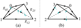
Figure 5: (Color online) Two branched simplices with opposite orientations. (a) A branched simplex with positive orientation and (b) a branched simplex with negative orientation.

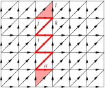
Figure 6: (Color online) A 1-cochain $a$ has a value $1$ on the red links: $a_{ik}=a_{jk}=1$ and a value $0$ on other links: $a_{ij}=a_{kl}=0$. $\hskip 1.0pt\mathrm{d}a$ is non-zero on the shaded triangles: $(\hskip 1.0pt\mathrm{d}a)_{jkl}=a_{jk}+a_{kl}-a_{jl}$. For such 1-cohain, we also have $a\smile a=0$. So when viewed as a $\mathbb{Z}_{2}$-valued cochain, $\beta_{2}a\neq a\smile a$ mod 2.

We like to remark that a simplex $(i,j,\cdots,k)$ can have two different orientations. We can use $(i,j,\cdots,k)$ and $(j,i,\cdots,k)=-(i,j,\cdots,k)$ to denote the same simplex with opposite orientations. The value $f_{n;i,j,\cdots,k}$ assigned to the simplex with opposite orientations should differ by a sign: $f_{n;i,j,\cdots,k}=-f_{n;j,i,\cdots,k}$. So to be more precise $f_{n}$ is a linear map $f_{n}:n\text{-simplex}\to\mathbb{M}$. We can denote the linear map as $\langle f_{n},n\text{-simplex}\rangle$, or

$$\langle f_{n},(i,j,\cdots,k)\rangle=f_{n;i,j,\cdots,k}\in\mathbb{M}.$$ (184)

More generally, a cochain $f_{n}$ is a linear map of $n$-chains:

$$f_{n}:n\text{-chains}\to\mathbb{M},$$ (185)

or (see Fig. 6)

$$\langle f_{n},n\text{-chain}\rangle\in\mathbb{M},$$ (186)

where a chain is a composition of simplices. For example, a 2-chain can be a 2-simplex: $(i,j,k)$, a sum of two 2-simplices: $(i,j,k)+(j,k,l)$, a more general composition of 2-simplices: $(i,j,k)-2(j,k,l)$, etc. The map $f_{n}$ is linear respect to such a composition. For example, if a chain is $m$ copies of a simplex, then its assigned value will be $m$ times that of the simplex. $m=-1$ correspond to an opposite orientation.

We will use $C^{n}({\cal M}^{D};\mathbb{M})$ to denote the set of all $n$-cochains on ${\cal M}^{D}$. $C^{n}({\cal M}^{D};\mathbb{M})$ can also be viewed as a set all $\mathbb{M}$-valued fields (or paths) on ${\cal M}^{D}$. Note that $C^{n}({\cal M}^{D};\mathbb{M})$ is an Abelian group under the $+$-operation.

The total spacetime lattice ${\cal M}^{D}$ correspond to a $D$-chain. We will use the same ${\cal M}^{D}$ to denote it. Viewing $f_{D}$ as a linear map of $D$-chains, we can define an “integral” over ${\cal M}^{D}$:

$$\int_{{\cal M}^{D}}f_{D} \equiv\langle f_{D},{\cal M}^{D}\rangle$$ (187)

$$=\sum_{(i_{0},i_{1},\cdots,i_{D})}s_{i_{0}i_{1}\cdots i_{D}}(f_{D})_{i_{0},i_{1},\cdots,i_{D}}.$$

Here $s_{i_{0}i_{1}\cdots i_{D}}=\pm 1$, such that a $D$-simplex in the $D$-chain ${\cal M}^{D}$ is given by $s_{i_{0}i_{1}\cdots i_{D}}(i_{0},i_{1},\cdots,i_{D})$.

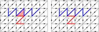
Figure 7: (Color online) A 1-cochain $a$ has a value $1$ on the red links, Another 1-cochain $a^{\prime}$ has a value $1$ on the blue links. On the left, $a\smile a^{\prime}$ is non-zero on the shade triangles: $(a\smile a^{\prime})_{ijl}=a_{ij}a^{\prime}_{jl}=1$. On the right, $a^{\prime}\smile a$ is zero on every triangle. Thus $a\smile a^{\prime}+a^{\prime}\smile a$ is not a coboundary.

We can define a derivative operator $\hskip 1.0pt\mathrm{d}$ acting on an $n$-cochain $f_{n}$, which give us an $(n+1)$-cochain (see Fig. 6):

$$\ \ \ \ \langle\hskip 1.0pt\mathrm{d}f_{n},(i_{0}i_{1}i_{2}\cdots i_{n+1})\rangle$$

$$=\sum_{m=0}^{n+1}(-)^{m}\langle f_{n},(i_{0}i_{1}i_{2}\cdots\hat{i}_{m}\cdots i_{n+1})\rangle$$ (188)

where $i_{0}i_{1}i_{2}\cdots\hat{i}_{m}\cdots i_{n+1}$ is the sequence $i_{0}i_{1}i_{2}\cdots i_{n+1}$ with $i_{m}$ removed, and $i_{0},i_{1},i_{2}\cdots i_{n+1}$ are the ordered vertices of the $(n+1)$-simplex $(i_{0}i_{1}i_{2}\cdots i_{n+1})$.

A cochain $f_{n}\in C^{n}({\cal M}^{D};\mathbb{M})$ is called a cocycle if $\hskip 1.0pt\mathrm{d}f_{n}=0$. The set of cocycles is denoted by $Z^{n}({\cal M}^{D};\mathbb{M})$. A cochain $f_{n}$ is called a coboundary if there exist a cochain $f_{n-1}$ such that $\hskip 1.0pt\mathrm{d}f_{n-1}=f_{n}$. The set of coboundaries is denoted by $B^{n}({\cal M}^{D};\mathbb{M})$. Both $Z^{n}({\cal M}^{D};\mathbb{M})$ and $B^{n}({\cal M}^{D};\mathbb{M})$ are Abelian groups as well. Since $\hskip 1.0pt\mathrm{d}^{2}=0$, a coboundary is always a cocycle: $B^{n}({\cal M}^{D};\mathbb{M})\subset Z^{n}({\cal M}^{D};\mathbb{M})$. We may view two cocycles differ by a coboundary as equivalent. The equivalence classes of cocycles, $[f_{n}]$, form the so called cohomology group denoted by

$$H^{n}({\cal M}^{D};\mathbb{M})=Z^{n}({\cal M}^{D};\mathbb{M})/B^{n}({\cal M}^{D};\mathbb{M}),$$ (189)

$H^{n}({\cal M}^{D};\mathbb{M})$, as a group quotient of $Z^{n}({\cal M}^{D};\mathbb{M})$ by $B^{n}({\cal M}^{D};\mathbb{M})$, is also an Abelian group.

For the $\mathbb{Z}_{N}$-valued cocycle $x_{n}$, $\hskip 1.0pt\mathrm{d}x_{n}\overset{\scriptscriptstyle N}{=}0$. Thus

$$\beta_{N}x_{n}\equiv\frac{1}{N}\hskip 1.0pt\mathrm{d}x_{n}$$ (190)

is a $\mathbb{Z}$-valued cocycle. Here $\beta_{N}$ is Bockstrin homomorphism.

We notice the above definition for cochains still makes sense if we have a non-Abelian group $(G,\cdot)$ instead of an Abelian group $(\mathbb{M},+)$, however the differential $\hskip 1.0pt\mathrm{d}$ defined by eqn. (A) will not satisfy $\hskip 1.0pt\mathrm{d}\circ\hskip 1.0pt\mathrm{d}=1$, except for the first two $\hskip 1.0pt\mathrm{d}$’s. That is, one may still make sense of 0-cocycle and 1-cocycle, but no more further naively by formula eqn. (A). For us, we only use non-Abelian 1-cocycle in this article. Thus it is ok. Non-Abelian cohomology is then thoroughly studied in mathematics motivating concepts such as gerbes to enter.

From two cochains $f_{m}$ and $h_{n}$, we can construct a third cochain $p_{m+n}$ via the cup product (see Fig. 7):

$$p_{m+n} =f_{m}\smile h_{n},$$

$$\langle p_{m+n},(0\to{m+n})\rangle =\langle f_{m},(0\to m)\rangle\times$$

$$\ \ \ \ \langle h_{n},(m\to{m+n})\rangle,$$ (191)

where $i\to j$ is the consecutive sequence from $i$ to $j$:

$$i\to j\equiv i,i+1,\cdots,j-1,j.$$ (192)

Note that the above definition applies to cochains with global.

The cup product has the following property

$$\hskip 1.0pt\mathrm{d}(h_{n}\smile f_{m}) =(\hskip 1.0pt\mathrm{d}h_{n})\smile f_{m}+(-)^{n}h_{n}\smile(\hskip 1.0pt\mathrm{d}f_{m})$$ (193)

for cochains with global or local values. We see that $h_{n}\smile f_{m}$ is a cocycle if both $f_{m}$ and $h_{n}$ are cocycles. If both $f_{m}$ and $h_{n}$ are cocycles, then $f_{m}\smile h_{n}$ is a coboundary if one of $f_{m}$ and $h_{n}$ is a coboundary. So the cup product is also an operation on cohomology groups $\underset{{\scriptscriptstyle}}{\smile}:H^{m}(M^{D};\mathbb{M})\times H^{n}(M^{D};\mathbb{M})\to H^{m+n}(M^{D};\mathbb{M})$. The cup product of two cocycles has the following property (see Fig. 7)

$$f_{m}\smile h_{n} =(-)^{mn}h_{n}\smile f_{m}+\text{coboundary}$$ (194)

We can also define higher cup product $f_{m}\underset{{\scriptscriptstyle k}}{\smile}h_{n}$ which gives rise to a $(m+n-k)$-cochain Steenrod (1947):

$$\ \ \ \ \langle f_{m}\underset{{\scriptscriptstyle k}}{\smile}h_{n},(0,1,\cdots,m+n-k)\rangle$$

$$=\hskip-10.00002pt\sum_{0\leq i_{0}<\cdots<i_{k}\leq n+m-k}\hskip-30.00005pt(-)^{p}\langle f_{m},(0\to i_{0},i_{1}\to i_{2},\cdots)\rangle\times$$

$$\ \ \ \ \ \ \ \ \ \ \ \ \ \ \ \ \ \ \ \ \langle h_{n},(i_{0}\to i_{1},i_{2}\to i_{3},\cdots)\rangle,$$ (195)

and $f_{m}\underset{{\scriptscriptstyle k}}{\smile}h_{n}=0$ for $k<0$ or for $k>m\text{ or }n$. Here $i\to j$ is the sequence $i,i+1,\cdots,j-1,j$, and $p$ is the number of permutations to bring the sequence

$$0\to i_{0},i_{1}\to i_{2},\cdots;i_{0}+1\to i_{1}-1,i_{2}+1\to i_{3}-1,\cdots$$ (196)

to the sequence

$$0\to m+n-k.$$ (197)

For example

$$\langle f_{m}\underset{{\scriptscriptstyle 1}}{\smile}h_{n},(0\to m+n-1)\rangle=\sum_{i=0}^{m-1}(-)^{(m-i)(n+1)}\times$$

$$\langle f_{m},(0\to i,i+n\to m+n-1)\rangle\langle h_{n},(i\to i+n)\rangle.$$ (198)

We can see that $\underset{{\scriptscriptstyle 0}}{\smile}=\smile$. Unlike cup product at $k=0$, the higher cup product of two cocycles may not be a cocycle. For cochains $f_{m},h_{n}$, we have

$$\hskip 1.0pt\mathrm{d}(f_{m}\underset{{\scriptscriptstyle k}}{\smile}h_{n})=\hskip 1.0pt\mathrm{d}f_{m}\underset{{\scriptscriptstyle k}}{\smile}h_{n}+(-)^{m}f_{m}\underset{{\scriptscriptstyle k}}{\smile}\hskip 1.0pt\mathrm{d}h_{n}+$$ (199)

$$\ \ \ (-)^{m+n-k}f_{m}\underset{{\scriptscriptstyle k-1}}{\smile}h_{n}+(-)^{mn+m+n}h_{n}\underset{{\scriptscriptstyle k-1}}{\smile}f_{m}$$

Let $f_{m}$ and $h_{n}$ be cocycles and $c_{l}$ be a chain, from eqn. (199) we can obtain

$$\hskip 1.0pt\mathrm{d}(f_{m}\underset{{\scriptscriptstyle k}}{\smile}h_{n})=(-)^{m+n-k}f_{m}\underset{{\scriptscriptstyle k-1}}{\smile}h_{n}$$

$$\ \ \ \ \ \ \ \ \ \ \ \ \ \ \ \ \ +(-)^{mn+m+n}h_{n}\underset{{\scriptscriptstyle k-1}}{\smile}f_{m},$$

$$\hskip 1.0pt\mathrm{d}(f_{m}\underset{{\scriptscriptstyle k}}{\smile}f_{m})=[(-)^{k}+(-)^{m}]f_{m}\underset{{\scriptscriptstyle k-1}}{\smile}f_{m},$$

$$\hskip 1.0pt\mathrm{d}(c_{l}\underset{{\scriptscriptstyle k-1}}{\smile}c_{l}+c_{l}\underset{{\scriptscriptstyle k}}{\smile}\hskip 1.0pt\mathrm{d}c_{l})=\hskip 1.0pt\mathrm{d}c_{l}\underset{{\scriptscriptstyle k}}{\smile}\hskip 1.0pt\mathrm{d}c_{l}$$

$$\ \ \ -[(-)^{k}-(-)^{l}](c_{l}\underset{{\scriptscriptstyle k-2}}{\smile}c_{l}+c_{l}\underset{{\scriptscriptstyle k-1}}{\smile}\hskip 1.0pt\mathrm{d}c_{l}).$$ (200)

From eqn. (A), we see that, for $\mathbb{Z}_{2}$-valued cocycles $z_{n}$,

$$\text{Sq}^{n-k}(z_{n})\equiv z_{n}\underset{{\scriptscriptstyle k}}{\smile}z_{n}$$ (201)

is always a cocycle. Here Sq is called the Steenrod square. More generally $h_{n}\underset{{\scriptscriptstyle k}}{\smile}h_{n}$ is a cocycle if $n+k=$ odd and $h_{n}$ is a cocycle. Usually, the Steenrod square is defined only for $\mathbb{Z}_{2}$-valued cocycles or cohomology classes. Here, we like to define a generalized Steenrod square for $\mathbb{M}$-valued cochains $c_{n}$:

$$\mathbb{Sq}^{n-k}c_{n}\equiv c_{n}\underset{{\scriptscriptstyle k}}{\smile}c_{n}+c_{n}\underset{{\scriptscriptstyle k+1}}{\smile}\hskip 1.0pt\mathrm{d}c_{n}.$$ (202)

From eqn. (A), we see that

$$\hskip 1.0pt\mathrm{d}\mathbb{Sq}^{k}c_{n} =\hskip 1.0pt\mathrm{d}(c_{n}\underset{{\scriptscriptstyle n-k}}{\smile}c_{n}+c_{n}\underset{{\scriptscriptstyle n-k+1}}{\smile}\hskip 1.0pt\mathrm{d}c_{n})$$ (203)

$$=\mathbb{Sq}^{k}\hskip 1.0pt\mathrm{d}c_{n}+(-)^{n}\begin{cases}0,&k=\text{odd}\\ 2\mathbb{Sq}^{k+1}c_{n}&k=\text{even}\\ \end{cases}.$$

In particular, when $c_{n}$ is a $\mathbb{Z}_{2}$-valued cochain, we have

$$\hskip 1.0pt\mathrm{d}\mathbb{Sq}^{k}c_{n}\overset{\scriptscriptstyle 2}{=}\mathbb{Sq}^{k}\hskip 1.0pt\mathrm{d}c_{n}.$$ (204)

Next, let us consider the action of $\mathbb{Sq}^{k}$ on the sum of two $\mathbb{M}$-valued cochains $c_{n}$ and $c_{n}^{\prime}$:

$$\mathbb{Sq}^{k}(c_{n}+c_{n}^{\prime})=\mathbb{Sq}^{k}c_{n}+\mathbb{Sq}^{k}c_{n}^{\prime}+$$

$$\ \ \ c_{n}\underset{{\scriptscriptstyle n-k}}{\smile}c_{n}^{\prime}+c_{n}^{\prime}\underset{{\scriptscriptstyle n-k}}{\smile}c_{n}+c_{n}\underset{{\scriptscriptstyle n-k+1}}{\smile}\hskip 1.0pt\mathrm{d}c_{n}^{\prime}+c_{n}^{\prime}\underset{{\scriptscriptstyle n-k+1}}{\smile}\hskip 1.0pt\mathrm{d}c_{n}$$

$$=\mathbb{Sq}^{k}c_{n}+\mathbb{Sq}^{k}c_{n}^{\prime}+[1+(-)^{k}]c_{n}\underset{{\scriptscriptstyle n-k}}{\smile}c_{n}^{\prime}$$

$$\ \ \ -(-)^{n-k}[-(-)^{n-k}c_{n}^{\prime}\underset{{\scriptscriptstyle n-k}}{\smile}c_{n}+(-)^{n}c_{n}\underset{{\scriptscriptstyle n-k}}{\smile}c_{n}^{\prime}]$$

$$\ \ \ +c_{n}\underset{{\scriptscriptstyle n-k+1}}{\smile}\hskip 1.0pt\mathrm{d}c_{n}^{\prime}+c_{n}^{\prime}\underset{{\scriptscriptstyle n-k+1}}{\smile}\hskip 1.0pt\mathrm{d}c_{n}$$

$$=\mathbb{Sq}^{k}c_{n}+\mathbb{Sq}^{k}c_{n}^{\prime}+[1+(-)^{k}]c_{n}\underset{{\scriptscriptstyle n-k}}{\smile}c_{n}^{\prime}$$

$$+(-)^{n-k}[\hskip 1.0pt\mathrm{d}c_{n}^{\prime}\underset{{\scriptscriptstyle n-k+1}}{\smile}c_{n}+(-)^{n}c_{n}^{\prime}\underset{{\scriptscriptstyle n-k+1}}{\smile}\hskip 1.0pt\mathrm{d}c_{n}]$$

$$-(-)^{n-k}\hskip 1.0pt\mathrm{d}(c_{n}^{\prime}\underset{{\scriptscriptstyle n-k+1}}{\smile}c_{n})+c_{n}\underset{{\scriptscriptstyle n-k+1}}{\smile}\hskip 1.0pt\mathrm{d}c_{n}^{\prime}+c_{n}^{\prime}\underset{{\scriptscriptstyle n-k+1}}{\smile}\hskip 1.0pt\mathrm{d}c_{n}$$

$$=\mathbb{Sq}^{k}c_{n}+\mathbb{Sq}^{k}c_{n}^{\prime}+[1+(-)^{k}]c_{n}\underset{{\scriptscriptstyle n-k}}{\smile}c_{n}^{\prime}$$

$$\ \ \ +[1+(-)^{k}]c_{n}^{\prime}\underset{{\scriptscriptstyle n-k+1}}{\smile}\hskip 1.0pt\mathrm{d}c_{n}-(-)^{n-k}\hskip 1.0pt\mathrm{d}(c_{n}^{\prime}\underset{{\scriptscriptstyle n-k+1}}{\smile}c_{n})$$

$$\ \ \ -[(-)^{n-k+1}\hskip 1.0pt\mathrm{d}c_{n}^{\prime}\underset{{\scriptscriptstyle n-k+1}}{\smile}c_{n}-c_{n}\underset{{\scriptscriptstyle n-k+1}}{\smile}\hskip 1.0pt\mathrm{d}c_{n}^{\prime}]$$

$$=\mathbb{Sq}^{k}c_{n}+\mathbb{Sq}^{k}c_{n}^{\prime}+[1+(-)^{k}]c_{n}\underset{{\scriptscriptstyle n-k}}{\smile}c_{n}^{\prime}$$

$$\ \ \ +[1+(-)^{k}]c_{n}^{\prime}\underset{{\scriptscriptstyle n-k+1}}{\smile}\hskip 1.0pt\mathrm{d}c_{n}-(-)^{n-k}\hskip 1.0pt\mathrm{d}(c_{n}^{\prime}\underset{{\scriptscriptstyle n-k+1}}{\smile}c_{n})$$

$$\ \ \ -\hskip 1.0pt\mathrm{d}(\hskip 1.0pt\mathrm{d}c_{n}^{\prime}\underset{{\scriptscriptstyle n-k+2}}{\smile}c_{n})+\hskip 1.0pt\mathrm{d}c_{n}^{\prime}\underset{{\scriptscriptstyle n-k+2}}{\smile}\hskip 1.0pt\mathrm{d}c_{n}$$

$$=\mathbb{Sq}^{k}c_{n}+\mathbb{Sq}^{k}c_{n}^{\prime}+\hskip 1.0pt\mathrm{d}c_{n}^{\prime}\underset{{\scriptscriptstyle n-k+2}}{\smile}\hskip 1.0pt\mathrm{d}c_{n}$$

$$\ \ \ +[1+(-)^{k}][c_{n}\underset{{\scriptscriptstyle n-k}}{\smile}c_{n}^{\prime}+c_{n}^{\prime}\underset{{\scriptscriptstyle n-k+1}}{\smile}\hskip 1.0pt\mathrm{d}c_{n}]$$

$$\ \ \ -(-)^{n-k}\hskip 1.0pt\mathrm{d}(c_{n}^{\prime}\underset{{\scriptscriptstyle n-k+1}}{\smile}c_{n})-\hskip 1.0pt\mathrm{d}(\hskip 1.0pt\mathrm{d}c_{n}^{\prime}\underset{{\scriptscriptstyle n-k+2}}{\smile}c_{n}).$$ (205)

We see that, if one of the $c_{n}$ and $c_{n}^{\prime}$ is a cocycle,

$$\mathbb{Sq}^{k}(c_{n}+c_{n}^{\prime})\overset{\scriptscriptstyle 2,\hskip 1.0pt\mathrm{d}}{=}\mathbb{Sq}^{k}c_{n}+\mathbb{Sq}^{k}c_{n}^{\prime}.$$ (206)

We also see that

$$\ \ \ \ \mathbb{Sq}^{k}(c_{n}+\hskip 1.0pt\mathrm{d}f_{n-1})$$ (207)

$$=\mathbb{Sq}^{k}c_{n}+\mathbb{Sq}^{k}\hskip 1.0pt\mathrm{d}f_{n-1}+[1+(-)^{k}]\hskip 1.0pt\mathrm{d}f_{n-1}\underset{{\scriptscriptstyle n-k}}{\smile}c_{n}$$

$$\ \ \ -(-)^{n-k}\hskip 1.0pt\mathrm{d}(c_{n}\underset{{\scriptscriptstyle n-k+1}}{\smile}\hskip 1.0pt\mathrm{d}f_{n-1})-\hskip 1.0pt\mathrm{d}(\hskip 1.0pt\mathrm{d}c_{n}\underset{{\scriptscriptstyle n-k+2}}{\smile}\hskip 1.0pt\mathrm{d}f_{n-1})$$

$$=\mathbb{Sq}^{k}c_{n}+[1+(-)^{k}][\hskip 1.0pt\mathrm{d}f_{n-1}\underset{{\scriptscriptstyle n-k}}{\smile}c_{n}+(-)^{n}\mathbb{Sq}^{k+1}f_{n-1}]$$

$$+\hskip 1.0pt\mathrm{d}[\mathbb{Sq}^{k}f_{n-1}-(-)^{n-k}c_{n}\hskip-5.0pt\underset{{\scriptscriptstyle n-k+1}}{\smile}\hskip-5.0pt\hskip 1.0pt\mathrm{d}f_{n-1}-\hskip 1.0pt\mathrm{d}c_{n}\hskip-5.0pt\underset{{\scriptscriptstyle n-k+2}}{\smile}\hskip-5.0pt\hskip 1.0pt\mathrm{d}f_{n-1}]$$

$$=\mathbb{Sq}^{k}c_{n}+[1+(-)^{k}][c_{n}\underset{{\scriptscriptstyle n-k}}{\smile}\hskip 1.0pt\mathrm{d}f_{n-1}+(-)^{n}\mathbb{Sq}^{k+1}f_{n-1}]$$

$$+\hskip 1.0pt\mathrm{d}[\mathbb{Sq}^{k}f_{n-1}-(-)^{n-k}\hskip 1.0pt\mathrm{d}f_{n-1}\underset{{\scriptscriptstyle n-k+1}}{\smile}c_{n}].$$

Using eqn. (A), we can also obtain the following result if $\hskip 1.0pt\mathrm{d}c_{n}=\text{even}$

$$\ \ \ \ \mathbb{Sq}^{k}(c_{n}+2c_{n}^{\prime})$$

$$\overset{\scriptscriptstyle 4}{=}\mathbb{Sq}^{k}c_{n}+2\hskip 1.0pt\mathrm{d}(c_{n}\underset{{\scriptscriptstyle n-k+1}}{\smile}c_{n}^{\prime})+2\hskip 1.0pt\mathrm{d}c_{n}\underset{{\scriptscriptstyle n-k+1}}{\smile}c_{n}^{\prime}$$

$$\overset{\scriptscriptstyle 4}{=}\mathbb{Sq}^{k}c_{n}+2\hskip 1.0pt\mathrm{d}(c_{n}\underset{{\scriptscriptstyle n-k+1}}{\smile}c_{n}^{\prime})$$ (208)

As another application, we note that, for a $\mathbb{M}$-valued cochain $m_{d}$ and using eqn. (199),

$$\mathbb{Sq}^{1}(m_{d})=m_{d}\underset{{\scriptscriptstyle d-1}}{\smile}m_{d}+m_{d}\underset{{\scriptscriptstyle d}}{\smile}\hskip 1.0pt\mathrm{d}m_{d}$$

$$=\frac{1}{2}(-)^{d}[\hskip 1.0pt\mathrm{d}(m_{d}\underset{{\scriptscriptstyle d}}{\smile}m_{d})-\hskip 1.0pt\mathrm{d}m_{d}\underset{{\scriptscriptstyle d}}{\smile}m_{d}]+\frac{1}{2}m_{d}\underset{{\scriptscriptstyle d}}{\smile}\hskip 1.0pt\mathrm{d}m_{d}$$

$$=(-)^{d}\beta_{2}(m_{d}\underset{{\scriptscriptstyle d}}{\smile}m_{d})-(-)^{d}\beta_{2}m_{d}\underset{{\scriptscriptstyle d}}{\smile}m_{d}+m_{d}\underset{{\scriptscriptstyle d}}{\smile}\beta_{2}m_{d}$$

$$=(-)^{d}\beta_{2}\mathbb{Sq}^{0}m_{d}-2(-)^{d}\beta_{2}m_{d}\underset{{\scriptscriptstyle d+1}}{\smile}\beta_{2}m_{d}$$

$$=(-)^{d}\beta_{2}\mathbb{Sq}^{0}m_{d}-2(-)^{d}\mathbb{Sq}^{0}\beta_{2}m_{d}$$ (209)

This way, we obtain a relation between Steenrod square and Bockstein homomorphism, when $m_{d}$ is a $\mathbb{Z}_{2}$-valued cochain

$$\mathbb{Sq}^{1}(m_{d})\overset{\scriptscriptstyle 2}{=}\beta_{2}m_{d},$$ (210)

where we have used $\mathbb{Sq}^{0}m_{d}=m_{d}$ for $\mathbb{Z}_{2}$-valued cochain.

For a $k$-cochain $a_{k}$, $k=\text{odd}$, we find that

$$\ \ \ \ \mathbb{Sq}^{k}a_{k}=a_{k}a_{k}+a_{k}\underset{{\scriptscriptstyle 1}}{\smile}\hskip 1.0pt\mathrm{d}a_{k}$$ (211)

$$=\frac{1}{2}[\hskip 1.0pt\mathrm{d}a_{k}\underset{{\scriptscriptstyle 1}}{\smile}a_{k}-a_{k}\underset{{\scriptscriptstyle 1}}{\smile}\hskip 1.0pt\mathrm{d}a_{k}-\hskip 1.0pt\mathrm{d}(a_{k}\underset{{\scriptscriptstyle 1}}{\smile}a_{k})]+a_{k}\underset{{\scriptscriptstyle 1}}{\smile}\hskip 1.0pt\mathrm{d}a_{k}$$

$$=\frac{1}{2}[\hskip 1.0pt\mathrm{d}a_{k}\underset{{\scriptscriptstyle 2}}{\smile}\hskip 1.0pt\mathrm{d}a_{k}-\hskip 1.0pt\mathrm{d}(\hskip 1.0pt\mathrm{d}a_{k}\underset{{\scriptscriptstyle 2}}{\smile}a_{k})]-\frac{1}{2}\hskip 1.0pt\mathrm{d}(a_{k}\underset{{\scriptscriptstyle 1}}{\smile}a_{k})$$

$$=\frac{1}{4}\hskip 1.0pt\mathrm{d}(\hskip 1.0pt\mathrm{d}a_{k}\underset{{\scriptscriptstyle 3}}{\smile}\hskip 1.0pt\mathrm{d}a_{k})-\frac{1}{2}\hskip 1.0pt\mathrm{d}(a_{k}\underset{{\scriptscriptstyle 1}}{\smile}a_{k}+\hskip 1.0pt\mathrm{d}a_{k}\underset{{\scriptscriptstyle 2}}{\smile}a_{k})$$

Thus $\mathbb{Sq}^{k}a_{k}$ is always a $\mathbb{Q}$-valued conboundary, when $k$ is odd.

Appendix B Path integral and Hamiltonian

Figure 8: Each time-step of evolution is given by the path integral on a particular form of branched graph. Here is an example in 1+1D.

Consider a spacetime complex of topology $M_{\text{space}}\times I$ where $I=[t,t^{\prime}]$ represents the time dimension and $M_{\text{space}}$ is a closed space complex (see Fig. 8). The spacetime complex $M_{\text{space}}\times I$ has two boundaries: one at time $t$ and another at time $t^{\prime}$. A path integral on the spacetime complex $M_{\text{space}}\times I$ give us an amplitude $Z[\{g_{i}^{\prime},h_{ij}^{\prime},\cdots\},\{g_{i},h_{ij},\cdots\}]$ from a configuration $\{g_{i},h_{ij},\cdots\}$ at $t$ to another configuration $\{g_{i}^{\prime},h_{ij}^{\prime},\cdots\}$ at $t^{\prime}$. Here, $\{g_{i},h_{ij},\cdots\}$ and $\{g_{i}^{\prime},h_{ij}^{\prime},\cdots\}$ are the degrees of freedom on the boundaries (see Fig. 8). We like to interpret $Z[\{g_{i}^{\prime},h_{ij}^{\prime},\cdots\},\{g_{i},h_{ij},\cdots\}]$ as the amplitude of an evolution in imaginary time by a Hamiltonian:

$$\ \ \ \ Z[\{g_{i}^{\prime},h_{ij}^{\prime},\cdots\},\{g_{i},h_{ij},\cdots\}]$$

$$=\langle g_{i}^{\prime},h_{ij}^{\prime},\cdots|\hskip 1.0pt\mathrm{e}^{-(t^{\prime}-t)H}|g_{i},h_{ij},\cdots\rangle.$$ (212)

However, such an interpretation may not be valid since $Z[\{g_{i}^{\prime},h_{ij}^{\prime},\cdots\},\{g_{i},h_{ij},\cdots\}]$ may not give raise to a hermitian matrix.

To have a path integral that give rise to a hermitian matrix $H$, we require the path integral defined on the branched graphs to have a “reflection” property. The imaginary-time path integral (or partition function) has a form

$$Z=\sum_{\{g_{i}\},\{h_{ij}\},\cdots}\hskip 1.0pt\mathrm{e}^{-S(\{g_{i}\},\{h_{ij}\},\cdots)}$$ (213)

where the total action amplitude $\hskip 1.0pt\mathrm{e}^{-S}$ for a configuration $\{g_{i}\},\{h_{ij}\},\cdots$ (or a path) is given by

$$\hskip 1.0pt\mathrm{e}^{-S}=\prod_{(ij\cdots k)}[V_{ij\cdots k}(\{g_{i}\},\{h_{ij}\},\cdots)]^{s_{ij\cdots k}}.$$ (214)

Here $\prod_{(ij\cdots k)}$ is the product over all the $n$-cells $(ij\cdots k)$. Note that the contribution from an $n$-cell $(ij\cdots k)$ is $V_{ij\cdots k}(\{g_{i}\},\{h_{ij}\},\cdots)$ or $V^{*}_{ij\cdots k}(\{g_{i}\},\{h_{ij}\},\cdots)$ depending on the orientation $s_{ij\cdots k}$ of the cell (see Fig. 5).

Such a path integral give rise to the hermitian Hamiltonian evolution. The key is to require that each time-step of evolution is given by branched graphs of the form in Fig. 8. One can show that $Z[\{g_{i}^{\prime},h_{ij}^{\prime},\cdots\},\{g_{i},h_{ij},\cdots\}]$ obtained by summing over all in the internal indices in the branched graphs Fig. 8 has a form

$$\ \ \ \ Z[\{g_{i}^{\prime},h_{ij}^{\prime},\cdots\},\{g_{i},h_{ij},\cdots\}]$$ (215)

$$=\sum_{\{g_{i}^{\prime\prime},h_{ij}^{\prime\prime},\cdots\}}U^{*}[\{g_{i}^{\prime\prime},h_{ij}^{\prime\prime},\cdots\},\{g_{i}^{\prime},h_{ij}^{\prime},\cdots\}]$$

$$\ \ \ \ \ \ \ \ \ \ \ \ \ \ \ \ \ U[\{g_{i}^{\prime\prime},h_{ij}^{\prime\prime},\cdots\},\{g_{i},h_{ij},\cdots\}]$$

and represents a positive-definite hermitian matrix. Thus the path integral of the form (214) always correspond to a Hamiltonian evolution in imaginary time. In fact, the above $Z[\{g_{i}^{\prime},h_{ij}^{\prime},\cdots\},\{g_{i},h_{ij},\cdots\}]$ can be viewed as an imaginary-time evolution $T=\hskip 1.0pt\mathrm{e}^{-\Delta\tau H}$ for a single time step.

References

- Kitaev (2003) A. Y. Kitaev, Ann. Phys. (N.Y.) 303, 2 (2003).
- Wen (2003a) X.-G. Wen, Phys. Rev. Lett. 90, 016803 (2003a), quant-ph/0205004 .
- Levin and Wen (2003) M. Levin and X.-G. Wen, Phys. Rev. B 67, 245316 (2003), cond-mat/0302460 .
- Yoshida (2011) B. Yoshida, Annals of Physics 326, 15 (2011), arXiv:1007.4601 .
- Bombín (2014) H. Bombín, Communications in Mathematical Physics 327, 387 (2014), arXiv:1107.2707 .
- Wen (1989) X. G. Wen, Phys. Rev. B 40, 7387 (1989).
- Wen and Niu (1990) X. G. Wen and Q. Niu, Phys. Rev. B 41, 9377 (1990).
- Wen (1990) X. G. Wen, Int. J. Mod. Phys. B 04, 239 (1990).
- Nussinov and Ortiz (2009a) Z. Nussinov and G. Ortiz, Proceedings of the National Academy of Science 106, 16944 (2009a), arXiv:cond-mat/0605316 .
- Nussinov and Ortiz (2009b) Z. Nussinov and G. Ortiz, Annals of Physics 324, 977 (2009b), arXiv:cond-mat/0702377 .
- Gaiotto et al. (2015) D. Gaiotto, A. Kapustin, N. Seiberg, and B. Willett, Journal of High Energy Physics 2, 172 (2015), arXiv:1412.5148 .
- Hastings and Wen (2005) M. B. Hastings and X.-G. Wen, Phys. Rev. B 72, 045141 (2005), cond-mat/0503554 .
- Baez and Schreiber (2007) J. C. Baez and U. Schreiber, Contemp. Math. 431, AMS, Providence, Rhode Island , 7 (2007), math/0511710 .
- Girelli et al. (2008) F. Girelli, H. Pfeiffer, and E. M. Popescu, Journal of Mathematical Physics 49, 032503 (2008), arXiv:0708.3051 .
- Baez and Huerta (2011) J. C. Baez and J. Huerta, General Relativity and Gravitation 43, 2335 (2011), arXiv:1003.4485 .
- Kapustin and Thorngren (2013) A. Kapustin and R. Thorngren, (2013), arXiv:1309.4721 .
- Sharpe (2015) E. Sharpe, Fortschritte der Physik 63, 659 (2015), arXiv:1508.04770 .
- Thorngren and von Keyserlingk (2015) R. Thorngren and C. von Keyserlingk, (2015), arXiv:1511.02929 .
- Bullivant et al. (2017a) A. Bullivant, M. Calcada, Z. Kádár, P. Martin, and J. F. Martins, Phys. Rev. B95, 155118 (2017a), arXiv:1606.06639 .
- Costa de Almeida et al. (2017) R. Costa de Almeida, J. P. Ibieta-Jimenez, J. Lorca Espiro, and P. Teotonio-Sobrinho, (2017), arXiv:1711.04186 .
- Tachikawa (2017) Y. Tachikawa, (2017), arXiv:1712.09542 .
- Parzygnat (2018) A. J. Parzygnat, Two-dimensional algebra in lattice gauge theory, Ph.D. thesis, Connecticut U. (2018), arXiv:1802.01139 .
- Delcamp and Tiwari (2018) C. Delcamp and A. Tiwari, Journal of High Energy Physics 2018, 49 (2018), arXiv:1802.10104 .
- Lake (2018) E. Lake, (2018), arXiv:1802.07747 .
- Cordova et al. (2018) C. Cordova, T. T. Dumitrescu, and K. Intriligator, (2018), arXiv:1802.04790 .
- Hofman and Iqbal (2019) D. M. Hofman and N. Iqbal, SciPost Phys. 6, 006 (2019), arXiv:1802.09512 .
- Bouzid and Tahiri (2018) B. Bouzid and M. Tahiri, Acta Physica Polonica B 49, 1885 (2018), arXiv:1803.00529 .
- Benini et al. (2018) F. Benini, C. Cordova, and P.-S. Hsin, (2018), arXiv:1803.09336 .
- Nikolaus and Waldorf (2018) T. Nikolaus and K. Waldorf, (2018), arXiv:1804.00677 .
- Zhu et al. (2018) C. Zhu, T. Lan, and X.-G. Wen, (2018), arXiv:1808.09394 .
- Harlow and Ooguri (2018) D. Harlow and H. Ooguri, (2018), arXiv:1810.05338 .
- Wan and Wang (2018a) Z. Wan and J. Wang, (2018a), arXiv:1812.11968 .
- Wan and Wang (2018b) Z. Wan and J. Wang, (2018b), arXiv:1812.11967 .
- Guo et al. (2018) M. Guo, K. Ohmori, P. Putrov, Z. Wan, and J. Wang, (2018), arXiv:1812.11959 .
- Wan and Wang (2018c) Z. Wan and J. Wang, (2018c), arXiv:1812.11955 .
- Bullivant et al. (2017b) A. Bullivant, M. Calcada, Z. Kádár, J. F. Martins, and P. Martin, (2017b), arXiv:1702.00868 .
- Kobayashi et al. (2018) R. Kobayashi, K. Shiozaki, Y. Kikuchi, and S. Ryu, (2018), arXiv:1805.05367 .
- Zeng and Wen (2015) B. Zeng and X.-G. Wen, Phys. Rev. B 91, 125121 (2015), arXiv:1406.5090 .
- Swingle and McGreevy (2016) B. Swingle and J. McGreevy, Phys. Rev. B 93, 045127 (2016), arXiv:1407.8203 .
- Morandi (1997) P. J. Morandi, https://web.nmsu.edu/pamorand/notes/ (1997).
- Fannes et al. (1992) M. Fannes, B. Nachtergaele, and R. F. Werner, Commun. Math. Phys. 144, 443 (1992).
- Verstraete et al. (2005) F. Verstraete, J. I. Cirac, J. I. Latorre, E. Rico, and M. M. Wolf, Phys. Rev. Lett. 94, 140601 (2005), quant-ph/0410227 .
- Kitaev (2006) A. Kitaev, Annals of Physics 321, 2 (2006), cond-mat/0506438 .
- Rowell et al. (2009) E. Rowell, R. Stong, and Z. Wang, Comm. Math. Phys. 292, 343 (2009), arXiv:0712.1377 .
- Wen (2015a) X.-G. Wen, Nat. Sci. Rev. 3, 68 (2015a), arXiv:1506.05768 .
- Lan et al. (2016) T. Lan, L. Kong, and X.-G. Wen, Phys. Rev. B 94, 155113 (2016), arXiv:1507.04673 .
- Lan et al. (2018) T. Lan, L. Kong, and X.-G. Wen, Phys. Rev. X 8, 021074 (2018), arXiv:1704.04221 .
- Lan and Wen (2019) T. Lan and X.-G. Wen, Phys. Rev. X 9, 021005 (2019), arXiv:1801.08530 .
- Gu et al. (2015) Z.-C. Gu, Z. Wang, and X.-G. Wen, Phys. Rev. B 91, 125149 (2015), arXiv:1010.1517 .
- Kitaev (2001) A. Y. Kitaev, Phys.-Usp. 44, 131 (2001), cond-mat/0010440 .
- Levitov et al. (2001) L. S. Levitov, T. P. Orlando, J. B. Majer, and J. E. Mooij, (2001), cond-mat/0108266 .
- Chen et al. (2013) X. Chen, Z.-C. Gu, Z.-X. Liu, and X.-G. Wen, Phys. Rev. B 87, 155114 (2013), arXiv:1106.4772 .
- Wen (2013) X.-G. Wen, Phys. Rev. D 88, 045013 (2013), arXiv:1303.1803 .
- Gu and Wen (2009) Z.-C. Gu and X.-G. Wen, Phys. Rev. B 80, 155131 (2009), arXiv:0903.1069 .
- Chen et al. (2011a) X. Chen, Z.-X. Liu, and X.-G. Wen, Phys. Rev. B 84, 235141 (2011a), arXiv:1106.4752 .
- Wen (2015b) X.-G. Wen, Phys. Rev. B 91, 205101 (2015b), arXiv:1410.8477 .
- Wen (2017a) X.-G. Wen, Rev. Mod. Phys. 89, 041004 (2017a), arXiv:1610.03911 .
- Chen et al. (2010) X. Chen, Z.-C. Gu, and X.-G. Wen, Phys. Rev. B 82, 155138 (2010), arXiv:1004.3835 .
- Lu and Vishwanath (2013) Y.-M. Lu and A. Vishwanath, (2013), arXiv:1302.2634 .
- Chang et al. (2015) L. Chang, M. Cheng, S. X. Cui, Y. Hu, W. Jin, R. Movassagh, P. Naaijkens, Z. Wang, and A. Young, Journal of Physics A: Mathematical and Theoretical 48, 12FT01 (2015), arXiv:1412.6589 .
- Ye (2018) P. Ye, Phys. Rev. B 97, 125127 (2018), arXiv:1610.08645 .
- Chen et al. (2011b) X. Chen, Z.-C. Gu, and X.-G. Wen, Phys. Rev. B 83, 035107 (2011b), arXiv:1008.3745 .
- Schuch et al. (2011) N. Schuch, D. Perez-Garcia, and I. Cirac, Phys. Rev. B 84, 165139 (2011), arXiv:1010.3732 .
- Lan et al. (2017) T. Lan, L. Kong, and X.-G. Wen, Phys. Rev. B 95, 235140 (2017), arXiv:1602.05946 .
- Kapustin and Thorngren (2017) A. Kapustin and R. Thorngren, Journal of High Energy Physics 10, 80 (2017), arXiv:1701.08264 .
- Wang and Gu (2018) Q.-R. Wang and Z.-C. Gu, Phys. Rev. X8, 011055 (2018), arXiv:1703.10937 .
- Wang and Gu (2018) Q.-R. Wang and Z.-C. Gu, (2018), arXiv:1811.00536 .
- Kapustin and Thorngren (2014) A. Kapustin and R. Thorngren, (2014), arXiv:1404.3230 .
- ’t Hooft (1980) G. ’t Hooft, NATO Adv. Study Inst. Ser. B Phys. 59, 135 (1980).
- Kong et al. (2019) L. Kong, T. Lan, Y. Tian, and X.-G. Wen, to appear (2019).
- Levin and Wen (2005) M. A. Levin and X.-G. Wen, Phys. Rev. B 71, 045110 (2005), cond-mat/0404617 .
- Walker and Wang (2012) K. Walker and Z. Wang, Frontiers of Physics 7, 150 (2012), arXiv:1104.2632 .
- Bhardwaj et al. (2017) L. Bhardwaj, D. Gaiotto, and A. Kapustin, Journal of High Energy Physics 2017, 96 (2017), arXiv:1605.01640 .
- Williamson and Wang (2017) D. J. Williamson and Z. Wang, Annals of Physics 377, 311 (2017), arXiv:1606.07144 .
- Kong and Wen (2014) L. Kong and X.-G. Wen, (2014), arXiv:1405.5858 .
- Wen (2017b) X.-G. Wen, Phys. Rev. B 95, 205142 (2017b), arXiv:1612.01418 .
- Lan et al. (2018) T. Lan, C. Zhu, and X.-G. Wen, (2018), arXiv:1809.01112 .
- Wen and Wang (2018) X.-G. Wen and Z. Wang, (2018), arXiv:1801.09938 .
- Blok and Wen (1990) B. Blok and X.-G. Wen, Phys. Rev. B 42, 8145 (1990).
- Fröhlich and Kerler (1991) J. Fröhlich and T. Kerler, Nucl. Phys. B 354, 369 (1991).
- Wen and Zee (1992) X. G. Wen and A. Zee, Phys. Rev. B 46, 2290 (1992).
- DeMarco and Wen (2019) M. DeMarco and X.-G. Wen, to appear (2019).
- Beckman et al. (2002) D. Beckman, D. Gottesman, A. Kitaev, and J. Preskill, Phys. Rev. D 65, 065022 (2002), arXiv:hep-th/0110205 .
- Shi (2018) B. Shi, arXiv e-prints , arXiv:1810.01986 (2018), arXiv:1810.01986 .
- Huse et al. (2013) D. A. Huse, R. Nandkishore, V. Oganesyan, A. Pal, and S. L. Sondhi, Physical Review B 88, 014206 (2013), arXiv:1304.1158 .
- Bauer and Nayak (2013) B. Bauer and C. Nayak, Journal of Statistical Mechanics: Theory and Experiment 2013, 09005 (2013), arXiv:1306.5753 .
- Chandran et al. (2014) A. Chandran, V. Khemani, C. R. Laumann, and S. L. Sondhi, Physical Review B 89, 144201 (2014), arXiv:1310.1096 .
- Grozdanov et al. (2017) S. Grozdanov, D. M. Hofman, and N. Iqbal, Phys. Rev. D 95, 096003 (2017), arXiv:1610.07392 .
- Glorioso and Son (2018) P. Glorioso and D. T. Son, (2018), arXiv:1811.04879 .
- Motrunich and Senthil (2002) O. I. Motrunich and T. Senthil, Phys. Rev. Lett. 89, 277004 (2002).
- Wen (2003b) X.-G. Wen, Phys. Rev. B 68, 115413 (2003b), cond-mat/0210040 .
- Levin and Wen (2006) M. Levin and X.-G. Wen, Phys. Rev. B 73, 035122 (2006), hep-th/0507118 .
- Wess and Zumino (1971) J. Wess and B. Zumino, Phys. Lett. B 37, 95 (1971).
- Witten (1983) E. Witten, Nucl. Phys. B 223, 422 (1983).
- Costantino (2005) F. Costantino, Math. Z. 251, 427 (2005), math/0403014 .
- Chen et al. (2012) X. Chen, Z.-C. Gu, Z.-X. Liu, and X.-G. Wen, Science 338, 1604 (2012), arXiv:1301.0861 .
- Steenrod (1947) N. Steenrod, Annals of Mathematics 48, 290 (1947).