Sum Rate and Fairness Analysis for the MU-MIMO Downlink under PSK Signalling: Interference Suppression vs Exploitation

Abstract

In this paper, we analyze the sum rate performance of multi-user multiple-input multiple-output (MU-MIMO) systems, with a finite constellation phase-shift keying (PSK) input alphabet. We analytically calculate and compare the achievable sum rate in three downlink transmission scenarios: 1) without precoding, 2) with zero forcing (ZF) precoding 3) with closed form constructive interference (CI) precoding technique. In light of this, new analytical expressions for the average sum rate are derived in the three cases, and Monte Carlo simulations are provided throughout to validate the analysis. Furthermore, based on the derived expressions, a power allocation scheme that can ensure fairness among the users is also proposed. The results in this work demonstrate that, the CI strictly outperforms the other two schemes, and the performance gap between the considered schemes increases with increase in the MIMO size. In addition, the CI provides higher fairness and the power allocation algorithm proposed in this paper can achieve maximum fairness index.

I Introduction

The recent decades have witnessed the widespread application of multi-user multiple-input multiple-output (MU-MIMO) communication systems, due to their high spectral efficiency and reliability [1, 2, 3]. However, these potential advantages of MU-MIMO systems are often undermined by strong interference in practical wireless systems [1, 2, 3]. Consequently, considerable amount of researches have focused on reducing/ mitigating the interference in MU-MIMO channels [3, 4, 5].

A number of information theoretic works have studied the sum rate performance of MU-MIMO systems by assuming Gaussian input signals. However, in practical communication systems, signals are generated from finite discrete constellation sets. In light of this, several works have considered MU-MIMO systems for finite alphabet input signals. In [3] optimal linear precoder for MU-MIMO interference channels with finite alphabet inputs was designed. In [5] the design of linear precoders in multi-cell MIMO systems for finite alphabet signals was studied. The authors in [6] considered the capacity of a MIMO fading channel with PSK input alphabet; in this work a downlink transmission without precoding was studied. In [7] the design of optimal precoders which maximize the mutual information of MIMO channels were investigated, by assuming non-Gaussian inputs of finite alphabet. The design of linear transmit precoder for MIMO broadcast channels with finite alphabet input signals was investigated in [8], where an explicit expression for the achievable rate region was derived. The work in [9] proposed low complexity precoding scheme that aimed to maximize the mutual information for MIMO systems with finite alphabet inputs. Linear precoder design that maximizes the average mutual information of MIMO fading channels with finite-alphabet inputs was proposed in [10], in which the statistical channel state information (CSI) was assumed to be known at the transmitter side. In [11], the authors studied a linear precoding for MIMO channels with finite discrete inputs, in which the capacity region for the MU-MIMO has been derived. In [12] a linear precoder design for MU-MIMO transceivers under finite alphabet inputs was proposed, where the optimal transmission strategies in both low and high signal-to-noise ratio (SNR) regions were studied. Although the aforementioned algorithms produced optimal performances, the fact that they have no closed form solutions and their resulting high computational complexity make them inapplicable in practical scenarios.

Recently, constructive interference (CI) precoding technique has been proposed to enhance the performance of downlink MU-MIMO systems [13, 14, 15, 16]. In contrast to the conventional techniques where the knowledge of the interference is used to cancel it, the main idea of the CI is to use the interference to improve the system performance. Specifically, the CI precoding technique exploits interference that can be known to the transmitter to increase the useful signal received power [13, 14, 15, 16]. That is, with the knowledge of the users’ data symbols and CSI, the interference can be classified as constructive and destructive. The interference signal is considered to be constructive to the transmitted signal if it moves the received symbols away from the decision thresholds of the constellation towards the direction of the desired symbol. Accordingly, the transmit precoding can be designed such that the resulting interference is constructive to the desired symbol.

The concept of the CI has been extensively studied in literature. This line of work has been introduced in [13], where the CI precoding scheme for the downlink of PSK-based MIMO systems has been proposed. In this work it was shown that the system performance can be enhanced by exploiting the interference signals. As a result, the effective signal to interference-plus-noise ratio (SINR) can be enhanced without the need to increase the transmitted signal power at the base station (BS). In [14] the concept of CI was used to design an optimization based precoder in the form of pre-scaling for the first time. Thereoff, [15] proposed transmit beamforming schemes for the MU-MIMO down-link that minimize the transmit power for generic PSK signals. In [16, 17] CI precoding scheme was applied in wireless power transfer scenario in order to minimize the transmit power while guaranteeing the energy harvesting and the quality of service (QoS) constraints for PSK messages. Further work in [18] applied the CI concept to massive multi-input multi-output (M-MIMO) systems. Very recently, the authors in [19] derived closed-form precoding expression for CI exploitation in the MU-MIMO down-link. The closed-form precoder in this work has for the first time made the application of CI exploitation practical, and has further paved the way for the development of communication theoretic analyses of the benefits of CI, which is the focus of this work.

Accordingly this paper investigates the sum rate of downlink transmission with finite constellation PSK signalling for interference suppression and interference exploitation techniques. Within this context, three transmission techniques are considered. The first is based on scenarios where the CSI is unknown at the BS, in which we study downlink transmission without precoding. The other two transmission schemes are based on full knowledge of the users’ CSI at the BS. In the second transmission scheme zero forcing (ZF) precoding technique is considered, and in the third scheme closed form CI precoding technique is analyzed for the first time. In this regard, explicit expressions for the average sum rate are derived in each transmission scheme. Then, based on the derived expressions the fairness among the users is also investigated.

For clarity we list the major contributions of this work as:

1. Firstly, new explicit analytical expressions for the average achievable rate upper bound of MU-MIMO with PSK inputs are derived for a) un-precoded transmission, b) ZF precoded transmission and c) CI precoded transmission, considering the channels to be of Rayleigh fading.

2. Based on the above analysis, a power allocation scheme that can provide fairness among the users is proposed.

3. The impact of the main system parameters on the system performance of the considered schemes are examined and investigated.

Results provided in this paper show that CI scheme outperforms the other two schemes, for the same system parameters. Also, it is shown that increasing the SNR and the number of the BS antennas enhances the system performance, whereas the gap between the minimum transmission power required for ZF and CI to achieve same target rate is almost fixed with increasing the distance between the BS and the users. Furthermore, the CI provides higher fairness than ZF and the power allocation algorithm proposed in this paper achieves high fairness index.

Next, Section II describes the system model under consideration. Sections III, IV, and V derive the analytical expressions for the average sum rate in conventional transmission, ZF and CI precoding techniques, respectively. Section VI, considers the users fairness in the three transmission schemes. Numerical and simulation results are presented and discussed in Section VII. Finally, the main conclusions of this work are stated in Section VIII.

Notations: $h$, $\mathbf{h}$, and $\mathbf{H}$ denote a scalar, a vector and a matrix, respectively. $(\cdot)^{H}$, $(\cdot)^{T}$ and $\textrm{diag}\left(.\right)$ denote conjugate transposition, transposition and diagonal of a matrix, respectively. $\mathcal{E}\left[.\right]$ denotes average operation. $\left[\mathbf{h}\right]_{k}$ denotes the $k^{th}$ element in $\mathbf{h}$ , $\left|.\right|$ denotes the absolute value, , and $\left\|.\right\|^{2}$ denotes the second norm. $\mathbb{C}^{K\times N}$ represents an K ×N matrix, and $\mathbf{I}$ denotes the identity matrix.

II System Model

Consider a downlink MU-MIMO system, consisting of a BS equipped with $N$ antennas communicating with $K$ single antenna users, where $N\geq K$. All the channels are modeled as independent identically distributed (i.i.d) Rayleigh fading channels. The channel matrix between the BS and the $K$ users is denoted by $\mathbf{H}\in\mathbb{C}^{K\times N}$, which can be represented as $\mathbf{H}=\mathbf{D}^{1/2}\mathbf{H}_{1}$where $\mathbf{H}_{1}\in\mathbb{C}^{K\times N}$ contains i.i.d $\mathcal{CN}\left(\text{0,}1\right)$ entries which represent small scale fading coefficients and $\mathbf{D}\in\mathbb{C}^{K\times K}$ is a diagonal matrix with $\left[\mathbf{D}\right]_{kk}=\varpi_{k}$ which represent the path-loss attenuation $\varpi_{k}=d_{k}^{-m}$, $d_{k}$ is the distance between the BS and the $k^{th}$ user and $m$ is the path loss exponent. It is also assumed that the signal is equiprobably drawn from an $M$-PSK constellation and denoted as $\mathbf{s}\in\mathbb{C}^{K\times 1}$ [19]. The received signal at the $k^{th}$ user can be expressed as,

$$y_{k}=\mathbf{h}_{k}\mathbf{W}\mathbf{s}+n_{k}$$ (1)

where $\mathbf{h}_{k}$ is the channel vector from the BS to user $k$, $\mathbf{W}$ is the precoding matrix, $n_{k}$ is the additive wight Gaussian noise (AWGN) at the $k^{th}$ user, $n_{k}\sim\mathcal{CN}\left(\text{0, }\sigma_{k}^{2}\right)$.

It was shown in [6, 12, 8] that, the achievable rate for the $k$-th user in general MU-MIMO system with finite constellation signaling, is given by,

$$R_{k}=N\log_{2}M-\frac{1}{M^{N}}\stackrel{{\scriptstyle[}}{{m}}=1]{M^{N}}{\sum}\mathcal{E}_{\mathbf{h,}\mathbf{n}}\left\{\log_{2}\stackrel{{\scriptstyle[}}{{i}}=1]{M^{N}}{\sum}e^{\frac{-\left\|\mathbf{h}_{k}\mathbf{W}\mathbf{\boldsymbol{s}}_{m,i}+n_{k}\right\|^{2}}{\sigma_{k}^{2}}}\right\}$$

$$+\frac{1}{M^{N-1}}\stackrel{{\scriptstyle[}}{{c}}=1]{M^{N-1}}{\sum}\mathcal{E}_{\mathbf{h,}\mathbf{n}}\left\{\log_{2}\stackrel{{\scriptstyle[}}{{t}}=1]{M^{N}}{\sum}e^{\frac{-\left\|\mathbf{h}_{k}\mathbf{W}\mathbf{\boldsymbol{s}}_{c,t}+n_{k}\right\|^{2}}{\sigma_{k}^{2}}}\right\},$$ (2)

where $\mathbf{s}_{m,i}=\mathbf{s}_{m}-\mathbf{s}_{i}$, $\mathbf{s}_{m}$ and $\mathbf{s}_{i}$ contain symbols taken from the $M$ signal constellation.

In the following, the average sum rate is derived for three cases, without precoding, with ZF precoding and with CI precoding technique.

III Downlink Transmission Without Precoding

In this case the BS transmits the users’ signals without any precoding technique, such scenario occurs when the CSI of the users is unknown at the BS. Let the $k^{th}$signal be equiprobably drawn from an $M$-PSK constellation, the average rate at a user $k$ can be written as [5, 12, 8],

$$\bar{R_{k}}=\log_{2}M^{N}-\underset{T_{1}}{\underbrace{\frac{1}{M^{N}}\stackrel{{\scriptstyle[}}{{m}}=1]{M^{N}}{\sum}\mathcal{E}_{\mathbf{h,}n_{k}}\log_{2}\stackrel{{\scriptstyle[}}{{i}}=1]{M^{N}}{\sum}e^{\frac{-\left|\sqrt{p_{N}}\mathbf{h}_{k}\mathbf{s}_{m,i}+n_{k}\right|^{2}}{\sigma_{k}^{2}}}}}$$

$$+\underset{T_{2}}{\underbrace{\frac{1}{M^{N-1}}\stackrel{{\scriptstyle[}}{{\underset{}}{missing}}{c\neq k}{c=1}]{M^{N-1}}{\sum}\mathcal{E}_{\mathbf{h,}n_{k}}\log_{2}\stackrel{{\scriptstyle[}}{{\underset{}}{missing}}{t\neq k}{t=1}]{M^{N-1}}{\sum}e^{\frac{-\left|\sqrt{p_{N}}\mathbf{h}_{k}\mathbf{s}_{c,t}+n_{k}\right|^{2}}{\sigma_{k}^{2}}}}},$$ (3)

where $p_{N}=\frac{p}{N}$, is the power transmitted by each antenna and $p$ is the total power transmission. The second and third terms in (3), $\left\{T_{1},T_{2}\right\}$, can be simplified to more familiar formulas. The second term, $T_{1}$, can be simplified by taking the $j^{th}$ term, $\left(e^{\frac{-\left|\sqrt{p_{N}}\mathbf{h}_{k}\mathbf{s}_{m,j}+n_{k}\right|^{2}}{\sigma_{k}^{2}}}\right)$, out as follows

$$T_{1}=\frac{1}{M^{N}}\stackrel{{\scriptstyle[}}{{m}}=1]{M^{N}}{\sum}\mathcal{E}_{\mathbf{h,}n_{k}}\left\{\log_{2}e^{\frac{-\left|\sqrt{p_{N}}\mathbf{h}_{k}\mathbf{s}_{m,j}+n_{k}\right|^{2}}{\sigma_{k}^{2}}}\right.$$

$$\times\left.\left(1+\stackrel{{\scriptstyle[}}{{i}}=1,i\neq j]{M^{N}}{\sum}e^{\frac{-\left|\sqrt{p_{N}}\mathbf{h}_{k}\mathbf{s}_{m,i}+n_{k}\right|^{2}+\left|\sqrt{p_{N}}\mathbf{h}_{k}\mathbf{s}_{m,j}+n_{k}\right|^{2}}{\sigma_{k}^{2}}}\right)\right\}$$ (4)

$$=\frac{1}{M^{N}}\stackrel{{\scriptstyle[}}{{m}}=1]{M^{N}}{\sum}\mathcal{E}_{\mathbf{h,}n_{k}}\left\{\left(\frac{-\left|\sqrt{p_{N}}\mathbf{h}_{k}\mathbf{s}_{m,j}+n_{k}\right|^{2}}{\sigma_{k}^{2}}\log_{2}e\right)\right.$$

$$\left.+\log_{2}\left(1+\stackrel{{\scriptstyle[}}{{i}}=1,i\neq j]{M^{N}}{\sum}e^{\frac{-\left|\sqrt{p_{N}}\mathbf{h}_{k}\mathbf{s}_{m,i}+n_{k}\right|^{2}+\left|\sqrt{p_{N}}\mathbf{h}_{k}\mathbf{s}_{m,j}+n_{k}\right|^{2}}{\sigma_{k}^{2}}}\right)\right\}.$$ (5)

where $j\in\left\{1:M^{N}\right\}$. Please note that, in case $j=m$, $e^{\frac{-\left|\sqrt{p_{N}}\mathbf{h}_{k}\mathbf{s}_{m,j}+n_{k}\right|^{2}}{\sigma_{k}^{2}}}=e^{\frac{-\left|n_{k}\right|^{2}}{\sigma_{k}^{2}}}$. Finally, with the use of some auxiliary notation the second term can be expressed as

$$T_{1}=\frac{1}{M^{N}}\stackrel{{\scriptstyle[}}{{m}}=1]{M^{N}}{\sum}\mathcal{E}_{\mathbf{h,}n_{k}}\left\{\left(\Upsilon_{1}+\log_{2}\left(1+\Xi_{1}\right)\right)\right\},$$ (6)

where $\Upsilon_{1}=\frac{-\left|\sqrt{p_{N}}\mathbf{h}_{k}\mathbf{s}_{m,j}+n_{k}\right|^{2}\log_{2}e}{\sigma_{k}^{2}}$ and $\Xi_{1}=\stackrel{{\scriptstyle[}}{{i}}=1,i\neq j]{M^{N}}{\sum}e^{\frac{-\left|\sqrt{p_{N}}\mathbf{h}_{k}\mathbf{s}_{m,i}+n_{k}\right|^{2}+\left|\sqrt{p_{N}}\mathbf{h}_{k}\mathbf{s}_{m,j}+n_{k}\right|^{2}}{\sigma_{k}^{2}}}.$ Likewise, by following similar steps for $T_{2}$ we can get

$$T_{2}=\frac{1}{M^{N-1}}\stackrel{{\scriptstyle[}}{{\underset{}}{missing}}{c\neq k}{c=1}]{M^{N-1}}{\sum}\mathcal{E}_{\mathbf{h,}n_{k}}\left\{\left(\Upsilon_{2}+\log_{2}\left(1+\Xi_{2}\right)\right)\right\},$$ (7)

where $\Upsilon_{2}=\frac{-\left|\sqrt{p_{N}}\mathbf{h}_{k}\mathbf{s}_{c,j}+n_{k}\right|^{2}\log_{2}e}{\sigma_{k}^{2}}$ and $\Xi_{2}=\stackrel{{\scriptstyle[}}{{t}}=1,t\neq k,j]{M^{N-1}}{\sum}e^{\frac{-\left|\sqrt{p_{N}}\mathbf{h}_{k}\mathbf{s}_{c,t}+n_{k}\right|^{2}+\left|\sqrt{p_{N}}\mathbf{h}_{k}\mathbf{s}_{c,j}+n_{k}\right|^{2}}{\sigma_{k}^{2}}}.$

Theorem 1.

The total sum rate upper-bound of the un-precoded downlink transmission scheme in MU-MIMO systems under PSK signaling can be calculated by

$$R=\stackrel{{\scriptstyle[}}{{k}}=1]{K}{\sum}\bar{R_{k}},$$ (8)

where $\bar{R_{k}}$ is given by (9), shown at the top of next page.

$$\bar{R_{k}} =N \log_{2}M-\frac{1}{M^{N}}\stackrel{{\scriptstyle[}}{{m}}=1]{M^{N}}{\sum}\left(-\log_{2}e\right.$$ (9)

$$\left.+\left\{\log_{2}\left(1+\stackrel{{\scriptstyle[}}{{i}}=1,i\neq j]{M^{N}}{\sum}\frac{2\sigma_{k}^{2}}{2\sigma_{k}^{2}+p_{N}d_{k}^{-m}\lambda_{mi}}\right)\right\}\right)+\frac{1}{M^{N-1}}\stackrel{{\scriptstyle[}}{{\underset{}}{missing}}{c\neq k}{c=1}]{M^{N-1}}{\sum}\left(-\log_{2}e\right.$$

$$\left.+\left\{\log_{2}\left(1+\stackrel{{\scriptstyle[}}{{t}}=1,t\neq k,j]{M^{N-1}}{\sum}\frac{2\sigma_{k}^{2}}{2\sigma_{k}^{2}+p_{N}d_{k}^{-m}\lambda_{ct}}\right)\right\}\right).$$

 

Proof:

In order to derive the average rate in this scenario, we need to find the averages of $T_{1}$ and $T_{2}$ over the noise and the channel states. To start with, the average of the first term in $T_{1}$, $\mathcal{E}_{\mathbf{h,}n_{k}}\left\{\Upsilon_{1}\right\}$, can be obtained as

$$\mathcal{E}_{\mathbf{h,}n_{k}}\left\{\frac{-\left|\sqrt{p_{N}}\mathbf{h}_{k}\mathbf{s}_{m,j}+n_{k}\right|^{2}}{\sigma_{k}^{2}}\log_{2}e\right\}$$

$$=\mathcal{E}_{\mathbf{h,}n_{k}}\left(\left|\sqrt{p_{N}}\mathbf{h}_{k}\mathbf{s}_{m,j}\right|^{2}+\left|n_{k}\right|^{2}+2\left(\left(\sqrt{p_{N}}\mathbf{h}_{k}\mathbf{s}_{m,j}\right)^{H}n_{k}\right)\right)\frac{-\log_{2}e}{\sigma_{k}^{2}}$$

$$=\mathcal{E}_{\mathbf{h}}\left\{-\left(\left|\sqrt{p_{N}}\mathbf{h}_{k}\mathbf{s}_{m,j}\right|^{2}+\sigma_{k}^{2}\right)\frac{\log_{2}e}{\sigma_{k}^{2}}\right\},$$

$$=-\left(p\varpi_{k}\left\|\mathbf{s}_{m,j}\right\|^{2}+\sigma_{k}^{2}\right)\frac{\log_{2}e}{\sigma_{k}^{2}}\qquad\qquad$$ (10)

which can be reduced to $-\log_{2}e,\textrm{ }$by choosing $j=m$. In order to calculate the average of the second term in $T_{1}$, since log is a concave function, we can apply Jensen’s inequality, which implicates that $\mathcal{E}\left\{\log\left(1+\Xi_{1}\right)\right\}\leq\log\left(1+\mathcal{E}\left\{\Xi_{1}\right\}\right)$[4]. Therefore, using Jensen inequality the upper bound can be obtained as

$$\mathcal{E}_{\mathbf{h,}n_{k}}\left\{\log_{2}\left(1+\stackrel{{\scriptstyle[}}{{i}}=1,i\neq j]{M^{N}}{\sum}e^{\frac{-\left|\sqrt{p_{N}}\mathbf{h}_{k}\mathbf{s}_{m,i}+n_{k}\right|^{2}+\left|\sqrt{p_{N}}\mathbf{h}_{k}\mathbf{s}_{m,j}+n_{k}\right|^{2}}{\sigma_{k}^{2}}}\right)\right\}\triangleq$$

$$\log_{2}\left(1+\stackrel{{\scriptstyle[}}{{i}}=1,i\neq j]{M^{N}}{\sum}\mathcal{E}_{\mathbf{h,}n_{k}}\left\{e^{\frac{-\left|\sqrt{p_{N}}\mathbf{h}_{k}\mathbf{s}_{m,i}+n_{k}\right|^{2}+\left|\sqrt{p_{N}}\mathbf{h}_{k}\mathbf{s}_{m,j}+n_{k}\right|^{2}}{\sigma_{k}^{2}}}\right\}\right).$$ (11)

Since $n_{k}$ has Gaussian distribution, the average over the noise can be derived as

$$\mathcal{E}_{n_{k}}\left\{e^{\frac{\left|\sqrt{p_{N}}\mathbf{h}_{k}\mathbf{s}_{m,j}+n_{k}\right|^{2}-\left|\sqrt{p_{N}}\mathbf{h}_{k}\mathbf{s}_{m,i}+n_{k}\right|^{2}}{\sigma_{k}^{2}}}\right\}=$$

$$\frac{1}{\pi\sigma^{2}}\underset{n_{k}}{\int}e^{-\frac{\left|\sqrt{p_{N}}\mathbf{h}_{k}\mathbf{s}_{m,i}+n_{k}\right|^{2}-\left|\sqrt{p_{N}}\mathbf{h}_{k}\mathbf{s}_{m,j}+n_{k}\right|^{2}+\left|n_{k}\right|^{2}}{\sigma_{k}^{2}}}dn_{k}.$$ (12)

Using the integrals of exponential function in [20], we can find

$$\mathcal{E}_{n_{k}}\left\{e^{\frac{\left|\sqrt{p_{N}}\mathbf{h}_{k}\mathbf{s}_{m,j}+n_{k}\right|^{2}-\left|\sqrt{p_{N}}\mathbf{h}_{k}\mathbf{s}_{m,i}+n_{k}\right|^{2}}{\sigma_{k}^{2}}}\right\}=$$

$$\qquad\qquad\qquad\qquad e^{-\frac{\left|\sqrt{p_{N}}\mathbf{h}_{k}\mathbf{s}_{m,i}\right|^{2}-\left|\sqrt{p_{N}}\mathbf{h}_{k}\mathbf{s}_{m,j}\right|^{2}}{2\sigma_{k}^{2}}}.$$ (13)

Therefore, the average over $\mathbf{h}$ can be written as,

$$\mathcal{E}_{\mathbf{h}}\left\{\mathcal{E}_{n_{k}}\left\{e^{\frac{\left|\sqrt{p_{N}}\mathbf{h}_{k}\mathbf{s}_{m,j}+n_{k}\right|^{2}-\left|\sqrt{p_{N}}\mathbf{h}_{k}\mathbf{s}_{m,i}+n_{k}\right|^{2}}{\sigma_{k}^{2}}}\right\}\right\}=$$

$$\mathcal{E}_{\mathbf{h}}\left\{e^{-\frac{\left|\sqrt{p_{N}}\mathbf{h}_{k}\mathbf{s}_{m,i}\right|^{2}-\left|\sqrt{p_{N}}\mathbf{h}_{k}\mathbf{s}_{m,j}\right|^{2}}{2\sigma_{k}^{2}}}\right\}.$$ (14)

Now, to derive the average over $\mathbf{h}$, it is more convenient to use the Quadratic form as follows

$$\varPhi_{i}=\left|\sqrt{p_{N}}\mathbf{h}_{k}\mathbf{s}_{m,i}\right|^{2}-\left|\sqrt{p_{N}}\mathbf{h}_{k}\mathbf{s}_{m,j}\right|^{2}$$

$$=p_{N}\mathbf{h}_{k}\underset{\mathbf{S}_{mi}}{\underbrace{\left(\mathbf{s}_{m,i}\mathbf{s}_{m,i}^{H}-\mathbf{s}_{m,j}\mathbf{s}_{m,j}^{H}\right)}}\mathbf{h}_{k}^{H},$$

$$=p_{N}\mathbf{h}_{k}\mathbf{S}_{mi}\mathbf{h}_{k}^{H}\qquad\qquad\qquad\qquad$$

$$=\stackrel{{\scriptstyle[}}{{n}}=1]{l}{\sum}p_{N}d_{k}^{-m}\lambda_{mi,n}\left|\mathbf{q}_{in}^{T}\mathbf{h}_{1k}\right|^{2},$$ (15)

where $\lambda_{mi,n}$ is the $n^{th}$ eigenvalue of matrix $\mathbf{S}_{mi}$ and $\mathbf{q}_{in}^{T}$ is the corresponding eigenvector. The distribution of $\varPhi_{i}$ depends on the number of the eigenvalues $\left(l\right)$ and the values of the eigenvalues. In case $l=1$, $\varPhi_{i}$ has exponential distribution, in case, $l>1$ $\varPhi_{i}$ has sum of exponential distributions, and in case all of the eigenvalues are ones and zeros, $\varPhi_{i}$ has Gamma distribution. By choosing $j=m$ the matrix $\mathbf{S}_{mi}$ will have one eigenvalue $\lambda_{mi}$. Therefore, $\varPhi_{i}$ will follow exponential distribution, and we can get,

$$\mathcal{E}_{\mathbf{\mathbf{h}}}\left\{e^{-\frac{\varPhi_{i}}{2\sigma_{k}^{2}}}\right\} = \stackrel{{\scriptstyle[}}{{0}}]{\infty}{\int}e^{-\frac{\varPhi}{2\sigma_{k}^{2}}}\,e^{-\varPhi}d\varPhi,$$ (16)

$$= \frac{2\sigma_{k}^{2}}{2\sigma_{k}^{2}+d_{k}^{-m}p_{N}\lambda_{mi}}.$$

Similarly, the average of the first term in $T_{2}$, $\mathcal{E}_{\mathbf{h,}n_{k}}\left\{\Upsilon_{2}\right\}$, can be obtained as

$$\mathcal{E}_{\mathbf{h,}n_{k}}\left\{\frac{-\left|\sqrt{p_{N}}\mathbf{h}_{k}\mathbf{s}_{c,j}+n_{k}\right|^{2}}{\sigma_{k}^{2}}\log_{2}e\right\}$$

$$=-\left(p\varpi_{k}\left\|\mathbf{s}_{c,j}\right\|^{2}+\sigma_{k}^{2}\right)\frac{\log_{2}e}{\sigma_{k}^{2}}.$$ (17)

which can be reduced to $-\log_{2}e,\textrm{ }$by choosing $c=j$. In order to derive the average of the second term in $T_{2}$, using Jensen’s inequality, $\mathcal{E}\left\{\log\left(1+\Xi_{2}\right)\right\}\leq\log\left(1+\mathcal{E}\left\{\Xi_{2}\right\}\right)$, we can calculate the upper bound as

$$\mathcal{E}_{\mathbf{h,}n_{k}}\left\{\log_{2}\left(1+\stackrel{{\scriptstyle[}}{{t}}=1,t\neq k,j]{M^{N-1}}{\sum}e^{\frac{-\left|\sqrt{p_{N}}\mathbf{h}_{k}\mathbf{s}_{c,t}+n_{k}\right|^{2}+\left|\sqrt{p_{N}}\mathbf{h}_{k}\mathbf{s}_{c,j}+n_{k}\right|^{2}}{\sigma_{k}^{2}}}\right)\right\}\triangleq$$

$$\log_{2}\left(1+\stackrel{{\scriptstyle[}}{{t}}=1,t\neq k,j]{M^{N-1}}{\sum}\mathcal{E}_{\mathbf{h,}n_{k}}\left\{e^{\frac{-\left|\sqrt{p_{N}}\mathbf{h}_{k}\mathbf{s}_{c,t}+n_{k}\right|^{2}+\left|\sqrt{p_{N}}\mathbf{h}_{k}\mathbf{s}_{c,j}+n_{k}\right|^{2}}{\sigma_{k}^{2}}}\right\}\right).$$ (18)

Since $n_{k}$ has Gaussian distribution, following similar steps as in (12) and (13), the average over the noise can be obtained as

$$\mathcal{E}_{n_{k}}\left\{e^{\frac{-\left|\sqrt{p_{N}}\mathbf{h}_{k}\mathbf{s}_{c,t}+n_{k}\right|^{2}+\left|\sqrt{p_{N}}\mathbf{h}_{k}\mathbf{s}_{c,j}+n_{k}\right|^{2}}{\sigma_{k}^{2}}}\right\}=$$

$$\qquad\qquad\qquad\qquad e^{-\frac{\left|\sqrt{p_{N}}\mathbf{h}_{k}\mathbf{s}_{c,t}\right|^{2}-\left|\sqrt{p_{N}}\mathbf{h}_{k}\mathbf{s}_{c,j}\right|^{2}}{2\sigma_{k}^{2}}}.$$ (19)

Now, the average over $\mathbf{h}$ can be written as,

$$\mathcal{E}_{\mathbf{h}}\left\{\mathcal{E}_{n_{k}}\left\{e^{\frac{-\left|\sqrt{p_{N}}\mathbf{h}_{k}\mathbf{s}_{c,t}+n_{k}\right|^{2}+\left|\sqrt{p_{N}}\mathbf{h}_{k}\mathbf{s}_{c,j}+n_{k}\right|^{2}}{\sigma_{k}^{2}}}\right\}\right\}=$$

$$\mathcal{E}_{\mathbf{h}}\left\{e^{-\frac{\left|\sqrt{p_{N}}\mathbf{h}_{k}\mathbf{s}_{c,t}\right|^{2}-\left|\sqrt{p_{N}}\mathbf{h}_{k}\mathbf{s}_{c,j}\right|^{2}}{2\sigma_{k}^{2}}}\right\}.$$ (20)

In order to derive the average over $\mathbf{h}$, the Quadratic form can be used as follows

$$\varPhi_{t}=\left|\sqrt{p_{N}}\mathbf{h}_{k}\mathbf{s}_{c,t}\right|^{2}-\left|\sqrt{p_{N}}\mathbf{h}_{k}\mathbf{s}_{c,j}\right|^{2}$$

$$=p_{N}\mathbf{h}_{k}\underset{\mathbf{S}_{ct}}{\underbrace{\left(\mathbf{s}_{c,t}\mathbf{s}_{c,t}^{H}-\mathbf{s}_{c,j}\mathbf{s}_{c,j}^{H}\right)}}\mathbf{h}_{k}^{H},$$

$$=p_{N}\mathbf{h}_{k}\mathbf{S}_{ct}\mathbf{h}_{k}^{H}\qquad\qquad\qquad\qquad$$

$$=\stackrel{{\scriptstyle[}}{{n}}=1]{l}{\sum}p_{N}d_{k}^{-m}\lambda_{ct,n}\left|\mathbf{q}_{tn}^{T}\mathbf{h}_{1k}\right|^{2}.$$ (21)

where $\lambda_{ct,n}$ is the $n^{th}$ eigenvalue of matrix $\mathbf{S}_{ct}$and $\mathbf{q}_{tn}^{T}$ is the corresponding eigenvector. The distribution of $\varPhi_{t}$ depends on the number of the eigenvalues $\left(l\right)$ and the values of the eigenvalues. By choosing $j=c$ the matrix $\mathbf{S}_{ct}$ will have one eigenvalue $\lambda_{ct}$, and then $\varPhi_{t}$ will follow exponential distribution. Therefore we can get,

$$\mathcal{E}_{\mathbf{\mathbf{h}}}\left\{e^{-\frac{\varPhi_{t}}{2\sigma_{k}^{2}}}\right\}=\frac{2\sigma_{k}^{2}}{2\sigma_{k}^{2}+p_{N}d_{k}^{-m}\lambda_{ct}}.$$ (22)

∎

The average sum-rate with respect to each user location can be obtained by averaging the derived sum-rate over all possible user locations.

IV Zero Forcing Precoding

In this case the BS has perfect CSI and ZF precoding technique is implemented. Therefore, the precoding matrix can be written as [21, 19],

$$\mathbf{W}\,=\frac{1}{\beta}\,\mathbf{H}^{H}\left(\mathbf{H}\mathbf{H}^{H}\right)^{-1},$$ (23)

where $\beta$ is the scaling factor to meet the transmit power constraint. Therefore, the received signal at the $k^{th}$ user can be expressed as,

$$y_{k} = \beta\mathbf{h}_{k}\mathbf{H}^{H}\left(\mathbf{H}\mathbf{H}^{H}\right)^{-1}\mathbf{s}+n_{k},$$ (24)

$$= \beta\left[\mathbf{s}\right]_{k}+n_{k}.$$

Consequently, the rate in this scenario is given by

$$\bar{R_{k}}^{ZF}=N\log_{2}M-\,\log_{2}e\quad\quad\quad\quad\quad\quad\quad\quad\quad$$

$$-\frac{1}{M^{N}}\stackrel{{\scriptstyle[}}{{m}}=1]{M^{N}}{\sum}\mathcal{E}_{\mathbf{H,}n_{k}}\left\{\log_{2}\stackrel{{\scriptstyle[}}{{i}}=1]{M^{N}}{\sum}e^{\frac{-\left|\beta\left[\mathbf{s}_{m,i}\right]_{k}+n_{k}\right|^{2}}{\sigma_{k}^{2}}}\right\}.$$ (25)

By taking the $j^{th}$ term $\left(e^{\frac{-\left|\beta\left[\mathbf{s}_{m,j}\right]_{k}+n_{k}\right|^{2}}{\sigma_{k}^{2}}}\right)$ out, (25) can be expressed as

$$\bar{R_{k}}^{ZF}=N\log_{2}M-\,\log_{2}e\quad\quad\quad\quad\quad\quad\quad\quad\quad\quad\quad\quad\quad\quad\quad$$

$$-\frac{1}{M^{N}}\stackrel{{\scriptstyle[}}{{m}}=1]{M^{N}}{\sum}\mathcal{E}_{\mathbf{H,}n_{k}}\left\{\left(\Upsilon+\log_{2}\left(1+\Xi\right)\right)\right\},$$ (26)

where $j\in\left[1,M^{N}\right]$ , $\Upsilon=\frac{-\left|\beta\left[\mathbf{s}_{m,j}\right]_{k}+n_{k}\right|^{2}}{\sigma_{k}^{2}}\log_{2}e$ and $\Xi=\stackrel{{\scriptstyle[}}{{i}}=1,i\neq j]{M^{N}}{\sum}e^{\frac{-\left|\beta\left[\mathbf{s}_{m,i}\right]_{k}+n_{k}\right|^{2}+\left|\beta\left[\mathbf{s}_{m,j}\right]_{k}+n_{k}\right|^{2}}{\sigma_{k}^{2}}}.$

Theorem 2.

The total sum rate upper-bound of the ZF transmission scheme in MU-MIMO systems under PSK signaling can be calculated by

$$R^{ZF}=\stackrel{{\scriptstyle[}}{{k}}=1]{K}{\sum}\bar{R_{k}}^{ZF},$$ (27)

where $\bar{R_{k}}^{ZF}$ is given by (28), shown at the top of next page.

$$\bar{R_{k}}^{ZF}=N\log_{2}M-\,\log_{2}e-\frac{1}{M^{N}}\stackrel{{\scriptstyle[}}{{m}}=1]{M^{N}}{\sum}\left\{\left(-\left(\left|\beta\left[\mathbf{s}_{m,j}\right]_{k}\right|^{2}+\sigma_{k}^{2}\right)\frac{\log_{2}e}{\sigma_{k}^{2}}\right)\right.$$

$$+\left.\log_{2}\left(1+\stackrel{{\scriptstyle[}}{{i}}=1,i\neq j]{M^{N}}{\sum}e^{-\frac{\left|\beta\left[\mathbf{s}_{m,i}\right]_{k}\right|^{2}-\left|\beta\left[\mathbf{s}_{m,j}\right]_{k}\right|^{2}}{2\sigma_{k}^{2}}}\right)\right\}$$ (28)

 

Proof:

To derive the average sum rate in this case, firstly we need to derive the average of the $\Upsilon$ term in (26). The scaling factor in this scenario is given by, $\beta=\sqrt{\frac{p}{\mathbf{s}^{H}\left(\mathbf{H}\mathbf{H}^{H}\right)^{-1}\mathbf{s}}}$[21, 19], where $p$ is the power transmission. For simplicity but without loss of generality, and in order to provide fair comparison between the considered schemes, in this paper we consider constant power scaling factors. It was shown that, the term, $X=\frac{\mathbf{s}^{H}\Sigma^{-1}\mathbf{s}}{\mathbf{s}^{H}\left(\mathbf{H}\mathbf{H}^{H}\right)^{-1}\mathbf{s}}$, follows Gamma distribution [22, 13], where $\Sigma=\mathbf{D}$, so the average of the scaling factor can be obtained as $\beta=\frac{\sqrt{\frac{p}{\mathbf{s}^{H}\Sigma^{-1}\mathbf{s}}}\Gamma\left(\frac{3}{2}-K+N\right)}{K\sqrt{K}\left(N-K\right)!}$. Therefore the average of term $\Upsilon$ in (26), $\mathcal{E}_{\mathbf{H,}n_{k}}\left\{\Upsilon\right\}$, can be obtained as

$$\mathcal{E}_{\mathbf{H,}n_{k}}\left\{\frac{-\left|\beta\left[\mathbf{s}_{m,j}\right]_{k}+n_{k}\right|^{2}}{\sigma_{k}^{2}}\log_{2}e\right\}=\quad\quad\quad\quad\quad\quad\quad\quad\quad$$

$$\quad\quad\left\{-\left(\left|\beta\left[\mathbf{s}_{m,j}\right]_{k}\right|^{2}+\sigma_{k}^{2}\right)\frac{\log_{2}e}{\sigma_{k}^{2}}\right\}.$$ (29)

Now, in order to calculate the average of the last term in (26), $\mathcal{E}_{\mathbf{H,}n_{k}}\left\{\log_{2}\left(1+\Xi\right)\right\}$, using Jensen inequality, the upper bound can be written as

$$\mathcal{E}_{\mathbf{H,}n_{k}}\left\{\log_{2}\left(1+\stackrel{{\scriptstyle[}}{{i}}=1,i\neq j]{M^{N}}{\sum}e^{\frac{-\left|\beta\left[\mathbf{s}_{m,i}\right]_{k}+n_{k}\right|^{2}+\left|\beta\left[\mathbf{s}_{m,j}\right]_{k}+n_{k}\right|^{2}}{\sigma_{k}^{2}}}\right)\right\}\triangleq$$

$$\log_{2}\left(1+\stackrel{{\scriptstyle[}}{{i}}=1,i\neq j]{M^{N}}{\sum}\mathcal{E}_{\mathbf{H,}n_{k}}\left\{e^{\frac{-\left|\beta\left[\mathbf{s}_{m,i}\right]_{k}+n_{k}\right|^{2}+\left|\beta\left[\mathbf{s}_{m,j}\right]_{k}+n_{k}\right|^{2}}{\sigma_{k}^{2}}}\right\}\right).$$ (30)

Since $n_{k}$ has Gaussian distribution, the average over $n_{k}$ can be derived as

$$\mathcal{E}_{n_{k}}\left\{e^{\frac{-\left|\beta\left[\mathbf{s}_{m,i}\right]_{k}+n_{k}\right|^{2}+\left|\beta\left[\mathbf{s}_{m,j}\right]_{k}+n_{k}\right|^{2}}{\sigma_{k}^{2}}}\right\}=$$

$$\frac{1}{\pi\sigma_{k}^{2}}\underset{n_{k}}{\int}e^{-\frac{\left|\beta\left[\mathbf{s}_{m,i}\right]_{k}+n_{k}\right|^{2}-\left|\beta\left[\mathbf{s}_{m,j}\right]_{k}+n_{k}\right|^{2}+\left|n_{k}\right|^{2}}{\sigma_{k}^{2}}}dn_{k}.$$ (31)

Using the integrals of exponential function in [20], we can find

$$\mathcal{E}_{n_{k}}\left\{e^{\frac{-\left|\beta\left[\mathbf{s}_{m,i}\right]_{k}+n_{k}\right|^{2}+\left|\beta\left[\mathbf{s}_{m,j}\right]_{k}+n_{k}\right|^{2}}{\sigma_{k}^{2}}}\right\}=$$

$$e^{-\frac{\left|\beta\left[\mathbf{s}_{m,i}\right]_{k}\right|^{2}-\left|\beta\left[\mathbf{s}_{m,j}\right]_{k}\right|^{2}}{2\sigma^{2}}}$$ (32)

∎

V Constructive Interference Precoding

The concept and characterization for the CI have been extensively investigated in MIMO systems [23, 24, 13]. In order to avoid repetition and for more details, we refer the reader to the aforementioned works in this paper. Here in this section, we analyze the performance of CI precoding technique in MU-MIMO systems, for the first time. We focus on the recent closed form CI precoding scheme, where the precoding matrix is given by [19],

$$\mathbf{W}\boldsymbol{s}=\frac{1}{K}\beta\,\mathbf{H}^{H}\left(\mathbf{H}\mathbf{H}^{H}\right)^{-1}\textrm{diag}\left\{\mathbf{V}^{-1}\mathbf{u}\right\}\mathbf{s},$$ (33)

where $\beta$ is the scaling factor to meet the transmit power constraint, which can be expressed as [19] $\beta=\sqrt{\frac{p}{\mathbf{u}^{H}\mathbf{V}^{-1}\mathbf{u}}},$ while $\mathbf{1}^{H}\mathbf{u}=\mathbf{1}$ and $\mathbf{V}=\textrm{diag}\left(\mathbf{s}^{H}\right)\left(\mathbf{H}\mathbf{H}^{H}\right)^{-1}\textrm{diag}\left(\mathbf{s}\right).$ For the sake of comparison, the normalization factor $\beta$ is designed to ensure that the long-term total transmit power at the source is constrained, and it is given by [4] $\beta=\sqrt{\frac{p}{\mathbf{u}^{H}\mathcal{E}\left[\mathbf{V}^{-1}\right]\mathbf{u}}},$ where $\mathcal{E}\left[\mathbf{V}^{-1}\right]=\textrm{diag}\left(\mathbf{s}^{H}\right)^{-1}\mathcal{E}\left[\left(\mathbf{H}\mathbf{H}^{H}\right)\right]\left(\textrm{diag}\left(\mathbf{s}\right)\right)^{-1}=\textrm{diag}\left(\mathbf{s}^{H}\right)^{-1}\,N\mathbf{\Sigma}\left(\textrm{diag}\left(\mathbf{s}\right)\right)^{-1}$ [25]. The received signal at the $k^{th}$ user now can be written as,

$$y_{k}=\frac{\beta}{K}\mathbf{h}_{k}\,\mathbf{H}^{H}\left(\mathbf{H}\mathbf{H}^{H}\right)^{-1}\textrm{diag}\left\{\mathbf{V}^{-1}\mathbf{u}\right\}\mathbf{s}+n_{k},\quad$$

$$=\frac{\beta}{K}\mathbf{a}_{k}\left(\textrm{diag}\left(\mathbf{s}^{H}\right)\right)^{-1}\mathbf{H}\mathbf{H}^{H}\left(\textrm{diag}\left(\mathbf{s}\right)\right)^{-1}\mathbf{u}\left[\boldsymbol{s}\right]_{k}+n_{k}$$ (34)

where $\mathbf{a}_{k}$ is a $1\times K$ vector all the elements of this vector are zeros except the $k^{th}$ element is one. Following the principles of CI, and the symmetric properties of the PSK constellation, the rate at the user $k$ can be written as,

$$\bar{R_{k}}^{CI}=N\log_{2}M-\,\log_{2}e\quad\quad\quad\quad\quad\quad\quad\quad\quad$$

$$-\frac{1}{M^{N}}\stackrel{{\scriptstyle[}}{{m}}=1]{M^{N}}{\sum}\mathcal{E}_{\mathbf{H,}n_{k}}\left\{\left(\Upsilon+\log_{2}\left(1+\Xi\right)\right)\right\},$$ (35)

wherewhere $\Upsilon=\frac{-\left|\mathbf{h}_{k}\mathbf{\mathbf{W}}\boldsymbol{s}_{m,j}+n_{k}\right|^{2}\log_{2}e}{\sigma_{k}^{2}}$ and

$\Xi=\stackrel{{\scriptstyle[}}{{i}}=1,i\neq j]{M^{N}}{\sum}e^{\frac{-\left|\mathbf{h}_{k}\mathbf{\mathbf{W}}\boldsymbol{s}_{m,i}+n_{k}\right|^{2}+\left|\mathbf{h}_{k}\mathbf{\mathbf{W}}\boldsymbol{s}_{m,j}+n_{k}\right|^{2}}{\sigma_{k}^{2}}}.$

Theorem 3.

The total sum rate upper-bound of the CI transmission scheme in MU-MIMO systems under PSK signaling can be calculated by

$$R^{CI}=\stackrel{{\scriptstyle[}}{{k}}=1]{K}{\sum}\bar{R_{k}}^{CI},$$ (36)

where

$$\bar{R_{k}}^{CI} = N\,\log_{2}M-\,\log_{2}e-\frac{1}{M^{N}}\stackrel{{\scriptstyle[}}{{m}}=1]{M^{N}}{\sum}\left(-\log_{2}e\right.$$ (37)

$$\left.+\left\{\log_{2}\left(1+\stackrel{{\scriptstyle[}}{{i}}=1,i\neq j]{M^{N}}{\sum}\Lambda_{m,i}\right)\right\}\right).$$

and $\Lambda_{m,i}$ is given by (38).

$$\Lambda_{m,i}=\left(\frac{2^{\left(\frac{1}{2}\left(N-K-1\right)\right)}K^{\left(N-K+1\right)}\left|\left[\boldsymbol{s}_{m,i}\right]_{k}\right|^{-2+K-N}}{\left(N-K\right)!}\right)\left(\left(\frac{c_{k}^{2}}{\sigma_{k}^{2}}\right)^{\frac{1}{2}\left(K-N-1\right)}\right)$$

$$\times\left(\left(c_{k}^{2}\left|\left[\boldsymbol{s}_{m,i}\right]_{k}\right|\right)\Gamma\left(\frac{1}{2}\left(N-K+1\right)\right)\textrm{${}_{1}\textrm{F}_{1}$}\left(\frac{1}{2}\left(N-K+1\right),\frac{1}{2},\frac{K^{2}\sigma_{k}^{2}}{2c_{k}^{2}\left|\left[\boldsymbol{s}_{m,i}\right]_{k}\right|^{2}}\right)\right.$$

$$\left.-\sqrt{2}K\,c_{k}\,\sigma_{k}\Gamma\left(\frac{1}{2}\left(N-K+2\right)\right){}_{1}\textrm{F}_{1}\left(\frac{1}{2}\left(N-K+2\right),\frac{3}{2},\frac{K^{2}\sigma_{k}^{2}}{2c_{k}^{2}\left|\left[\boldsymbol{s}_{m,i}\right]_{k}\right|^{2}}\right)\right).$$ (38)

 

Proof:

To start with, the average of the $\Upsilon$ term in (35), $\mathcal{E}_{\mathbf{H,}n_{k}}\left\{\Upsilon\right\}$ , can be obtained as

$$\mathcal{E}_{\mathbf{H,}n_{k}}\left\{\frac{-\left|\frac{\beta}{K}\left[\,\textrm{diag}\left\{\mathbf{V}^{-1}\mathbf{u}\right\}\boldsymbol{s}_{m,j}\right]_{k}+n_{k}\right|^{2}}{\sigma_{k}^{2}}\log_{2}e\right\}=$$

$$\mathcal{E}_{\mathbf{H}}\left\{-\left(\left|\frac{\beta}{K}\mathbf{a}_{k}\textrm{diag}\left\{\mathbf{V}^{-1}\mathbf{u}\right\}\left[\boldsymbol{s}_{m,j}\right]_{k}\right|^{2}+\sigma_{k}^{2}\right)\frac{\log_{2}e}{\sigma_{k}^{2}}\right\}.$$ (39)

In [25] it was shown that, the term $Z=\frac{\mathbf{a}_{k}\left(\textrm{diag}\left(\mathbf{s}^{H}\right)\right)^{-1}\left(\mathbf{H}\mathbf{H}^{H}\right)\left(\textrm{diag}\left(\mathbf{s}\right)\right)^{-1}\mathbf{u}\left[\boldsymbol{s}_{m,j}\right]_{k}}{\mathbf{a}_{k}\left(\textrm{diag}\left(\mathbf{s}^{H}\right)\right)^{-1}\left(\mathbf{\Sigma}\right)\left(\textrm{diag}\left(\mathbf{s}\right)\right)^{-1}\mathbf{u}\left[\boldsymbol{s}_{m,j}\right]_{k}}$ has Gamma distribution with $N$ degrees of freedom. Hence the average in (39) can be derived as in (40), shown at the top of next page.

$$\mathcal{E}_{\mathbf{H}}\left\{-\left(\left|\frac{\beta}{K}\mathbf{a}_{k}\textrm{diag}\left\{\mathbf{V}^{-1}\mathbf{u}\right\}\left[\boldsymbol{s}_{m,j}\right]_{k}\right|^{2}+\sigma_{k}^{2}\right)\frac{\log_{2}e}{\sigma_{k}^{2}}\right\}\quad\quad\quad\quad\quad\quad\quad\quad\quad\quad$$

$$=-\left(\mathcal{E}_{\mathbf{H}}\left\{\left|\frac{\beta\left(\mathbf{a}_{k}\left(\textrm{diag}\left(\mathbf{s}^{H}\right)\right)^{-1}\left(\mathbf{\Sigma}\right)\left(\textrm{diag}\left(\mathbf{s}\right)\right)^{-1}\mathbf{u}\left[\boldsymbol{s}_{m,j}\right]_{k}\right)}{K}Z\right|^{2}\right\}+\sigma_{k}^{2}\right)\frac{\log_{2}e}{\sigma_{k}^{2}}$$

$$\quad\quad\quad\quad=\left(\frac{-\Gamma\left(2+N\right)}{\sigma_{k}^{2}\Gamma\left(N\right)}\left|\frac{\beta\left(\mathbf{a}_{k}\left(\textrm{diag}\left(\mathbf{s}^{H}\right)\right)^{-1}\left(\mathbf{\Sigma}\right)\left(\textrm{diag}\left(\mathbf{s}\right)\right)^{-1}\mathbf{u}\left[\boldsymbol{s}_{m,j}\right]_{k}\right)}{K}\right|^{2}-1\right)\log_{2}e.$$ (40)

 

In order to calculate the average of the last term in (35), $\mathcal{E}_{\mathbf{H,}n_{k}}\left\{\log_{2}\left(1+\Xi\right)\right\}$, using Jensen inequality, the upper bound can be calculated as follows. Since $n_{k}$ has Gaussian distribution, the average over the noise can be obtained as

$$\mathcal{E}_{n_{k}}\left\{e^{\frac{-\left|\mathbf{h}_{k}\mathbf{\mathbf{W}}\boldsymbol{s}_{m,i}+n_{k}\right|^{2}+\left|\mathbf{h}_{k}\mathbf{\mathbf{W}}\boldsymbol{s}_{m,j}+n_{k}\right|^{2}}{\sigma_{k}^{2}}}\right\}$$

$$=e^{-\frac{\left|\frac{\beta}{K}\mathbf{a}_{k}\textrm{diag}\left\{\mathbf{V}^{-1}\mathbf{u}\right\}\boldsymbol{s}_{m,i}\right|^{2}-\left|\frac{\beta}{K}\mathbf{a}_{k}\textrm{diag}\left\{\mathbf{V}^{-1}\mathbf{u}\right\}\boldsymbol{s}_{m,j}\right|^{2}}{2\sigma_{k}^{2}}}.$$ (41)

Now, the average of (41) over $\mathbf{H}$ can be written as in (42), shown at the top of next page,

$$\mathcal{E}_{\mathbf{H}}\left\{e^{-\frac{\left|\frac{\beta}{K}\mathbf{a}_{k}\textrm{diag}\left\{\mathbf{V}^{-1}\mathbf{u}\right\}\boldsymbol{s}_{m,i}\right|^{2}-\left|\frac{\beta}{K}\mathbf{a}_{k}\textrm{diag}\left\{\mathbf{V}^{-1}\mathbf{u}\right\}\boldsymbol{s}_{m,j}\right|^{2}}{2\sigma_{k}^{2}}}\right\}\qquad\qquad\qquad\qquad\qquad\qquad\qquad\qquad$$

$$=\mathcal{E}_{\mathbf{H}}\left\{e^{-\frac{\left|\frac{\beta}{K}\mathbf{a}_{k}\left(\textrm{diag}\left(\mathbf{s}^{H}\right)\right)^{-1}\left(\mathbf{H}\mathbf{H}^{H}\right)\left(\textrm{diag}\left(\mathbf{s}\right)\right)^{-1}\mathbf{u}\left[\boldsymbol{s}_{m,i}\right]_{k}\right|^{2}-\left|\frac{\beta}{K}\,\mathbf{a}_{k}\left(\textrm{diag}\left(\mathbf{s}^{H}\right)\right)^{-1}\left(\mathbf{H}\mathbf{H}^{H}\right)\left(\textrm{diag}\left(\mathbf{s}\right)\right)^{-1}\mathbf{u}\left[\boldsymbol{s}_{m,j}\right]_{k}\right|^{2}}{2\sigma_{k}^{2}}}\right\},$$

$$=\mathcal{E}_{\mathbf{H}}\left\{e^{-\frac{\left|\frac{\beta\left(\mathbf{a}_{k}\left(\textrm{diag}\left(\mathbf{s}^{H}\right)\right)^{-1}\Sigma\left(\textrm{diag}\left(\mathbf{s}\right)\right)^{-1}\mathbf{u}\right)}{K}\,X\left[\boldsymbol{s}_{m,i}\right]_{k}\right|^{2}-\left|\frac{\beta\left(\mathbf{a}_{k}\left(\textrm{diag}\left(\mathbf{s}^{H}\right)\right)^{-1}\Sigma\left(\textrm{diag}\left(\mathbf{s}\right)\right)^{-1}\mathbf{u}\right)}{K}\,X\left[\boldsymbol{s}_{m,j}\right]_{k}\right|^{2}}{2\sigma_{k}^{2}}}\right\},$$

$$=\mathcal{E}_{\mathbf{H}}\left\{e^{-\frac{\chi_{i,j}}{2\sigma_{k}^{2}}}\right\}.\qquad\qquad\qquad\qquad\qquad\qquad\qquad\qquad\qquad\qquad\qquad\qquad\qquad\qquad$$ (42)

 

where $\chi_{i,j}=\left|\frac{\beta\left(\mathbf{a}_{k}\left(\textrm{diag}\left(\mathbf{s}^{H}\right)\right)^{-1}\Sigma\left(\textrm{diag}\left(\mathbf{s}\right)\right)^{-1}\mathbf{u}\right)}{K}\,X\left[\boldsymbol{s}_{m,i}\right]_{k}\right|^{2}-\left|\frac{\beta\left(\mathbf{a}_{k}\left(\textrm{diag}\left(\mathbf{s}^{H}\right)\right)^{-1}\Sigma\left(\textrm{diag}\left(\mathbf{s}\right)\right)^{-1}\mathbf{u}\right)}{K}\,X\left[\boldsymbol{s}_{m,j}\right]_{k}\right|^{2}$, $X=\frac{\mathbf{a}_{k}\left(\textrm{diag}\left(\mathbf{s}^{H}\right)\right)^{-1}\left(\mathbf{H}\mathbf{H}^{H}\right)\left(\textrm{diag}\left(\mathbf{s}\right)\right)^{-1}\mathbf{u}}{\mathbf{a}_{k}\left(\textrm{diag}\left(\mathbf{s}^{H}\right)\right)^{-1}\Sigma\left(\textrm{diag}\left(\mathbf{s}\right)\right)^{-1}\mathbf{u}}$ .

Since $\chi_{i,j}$ has Gamma distribution [22, 13]; we can find the average as in (43),

$$\mathcal{E}_{\mathbf{\mathbf{H}}}\left\{e^{-\frac{\chi_{i,j}}{2\sigma^{2}}}\right\}=\Lambda_{i,j}=\left(\frac{2^{\left(\frac{1}{2}\left(N-K-1\right)\right)}K^{\left(N-K+1\right)}}{\left(N-K\right)!}\right)\left(\left(\frac{c_{k}^{2}\xi}{\sigma_{k}^{2}}\right)^{\frac{1}{2}\left(K-N-1\right)}\right)$$

$$\quad\quad\quad\quad\quad\quad\quad\quad\times\left(\left(c_{k}^{2}\left(\left|\left[\boldsymbol{s}_{m,i}\right]_{k}\right|^{2}\right)\right)\Gamma\left(\frac{1}{2}\left(N-K+1\right)\right)\textrm{${}_{1}\textrm{F}_{1}$}\left(\frac{1}{2}\left(N-K+1\right),\frac{1}{2},\frac{K^{2}\sigma_{k}^{2}}{2c_{k}^{2}\xi}\right)\right.$$

$$\quad\quad\quad\quad\quad\quad\quad-\left(c_{k}^{2}\left(\left|\left[\boldsymbol{s}_{m,j}\right]_{k}\right|^{2}\right)\right)\Gamma\left(\frac{1}{2}\left(N-K+1\right)\right)\textrm{${}_{1}\textrm{F}_{1}$}\left(\frac{1}{2}\left(N-K+1\right),\frac{1}{2},\frac{K^{2}\sigma_{k}^{2}}{2c_{k}^{2}\xi}\right)$$

$$\left.\quad\quad\quad\quad\quad\quad\quad\quad\quad\quad\quad-\sqrt{2}K\,\sigma_{k}^{2}\sqrt{\frac{\xi}{\sigma_{k}^{2}}}\Gamma\left(\frac{1}{2}\left(N-K+2\right)\right){}_{1}\textrm{F}_{1}\left(\frac{1}{2}\left(N-K+2\right),\frac{3}{2},\frac{K^{2}\sigma_{k}^{2}}{2c_{k}^{2}\xi}\right)\right).$$ (43)

 

where $\xi=\left(\left|\left[\boldsymbol{s}_{m,i}\right]_{k}\right|^{2}-\left|\left[\boldsymbol{s}_{m,j}\right]_{k}\right|^{2}\right)$, $c_{k}=\frac{\beta\left(\mathbf{a}_{k}\left(\textrm{diag}\left(\mathbf{s}^{H}\right)\right)^{-1}\Sigma\left(\textrm{diag}\left(\mathbf{s}\right)\right)^{-1}\mathbf{u}\right)}{K}$ and ${}_{1}\textrm{F}_{1}$ is the Hypergeometric function. By choosing $j=m$, $\chi_{i,j}$ reduces to, $\chi_{i}=\left|\frac{\beta\left(\mathbf{a}_{k}\left(\textrm{diag}\left(\mathbf{s}^{H}\right)\right)^{-1}\Sigma\left(\textrm{diag}\left(\mathbf{s}\right)\right)^{-1}\mathbf{u}\right)}{K}\,X\left[\boldsymbol{s}_{m,i}\right]_{k}\right|^{2}$ and the expression can be further simplified as in (38). ∎

VI Fairness for MU-MIMO Systems with PSK Signaling

In this section we consider the fairness among the users for the system model under consideration. Firstly, based on the derived expressions in the previous sections, we calculate the minimum power required to achieve a target data rate, and then we propose a fairness algorithm that can be used to provide fairness in MU-MIMO systems with finite alphabet signals.

VI-A Minimum Power Transmission

Consider that the BS transmits the messages at a target data rate. Let the target data rate be denoted by $R_{T}$, so that for perfect transmission the achievable rate at the $k^{th}$ user, $\bar{R_{k}}$, has to satisfy the condition, $\bar{R_{k}}\geq R_{T}$ . In order to determine the minimum power transmission required to achieve $R_{T}$, we simplify the derived expressions in the previous sections as follows.

VI-A1 un-precoded downlink Transmission

To find the minimum power transmission in this case we simplify (9) into,

 

$$R_{T}=\bar{R_{k}}\quad\quad\quad\quad\quad\quad\quad\quad\quad\quad\quad\quad\quad\quad\quad\quad\quad\quad\quad\quad\quad\quad\quad\quad\quad\quad\quad$$

$$=X-\left\{\frac{1}{M^{N}}\stackrel{{\scriptstyle[}}{{m}}=1]{M^{N}}{\sum}\log_{2}\left(1+\stackrel{{\scriptstyle[}}{{i}}=1,i\neq j]{M^{N}}{\sum}\frac{2\sigma_{k}^{2}}{2\sigma_{k}^{2}+p_{k}d_{k}^{-m}\lambda_{mi}}\right)\right\}$$

$$+\left\{\frac{1}{M^{N-1}}\stackrel{{\scriptstyle[}}{{\underset{}}{missing}}{c\neq k}{c=1}]{M^{N-1}}{\sum}\log_{2}\left(1+\stackrel{{\scriptstyle[}}{{t}}=1,t\neq k]{M^{N-1}}{\sum}\frac{2\sigma_{k}^{2}}{2\sigma_{k}^{2}+p_{k}d_{k}^{-m}\lambda_{ct}}\right)\right\},$$ (44)

where $X=N\,\log_{2}M$. The minimum $p_{k}$ can be obtained by solving,

$$X-\left\{\frac{1}{M^{N}}\stackrel{{\scriptstyle[}}{{m}}=1]{M^{N}}{\sum}\log_{2}\left(1+\stackrel{{\scriptstyle[}}{{i}}=1,i\neq j]{M^{N}}{\sum}\frac{2\sigma_{k}^{2}}{2\sigma_{k}^{2}+p_{k}d_{k}^{-m}\lambda_{mi}}\right)\right\}+$$

$$\frac{1}{M^{N-1}}\stackrel{{\scriptstyle[}}{{\underset{}}{missing}}{c\neq k}{c=1}]{M^{N-1}}{\sum}\log_{2}\left(1+\stackrel{{\scriptstyle[}}{{\underset{}}{missing}}{t\neq k}{t=1}]{M^{N-1}}{\sum}\frac{2\sigma_{k}^{2}}{2\sigma_{k}^{2}+p_{k}d_{k}^{-m}\lambda_{ct}}\right)-R_{T}=0$$ (45)

Therefore, minimum value of $p_{k}$ is the value that satisfies (45). By exploiting the symmetric properties of the constellation [6, Eq(5)], (45) can be reduced to

$$X-\left\{\log_{2}\left(1+\stackrel{{\scriptstyle[}}{{i}}=1,i\neq j]{M^{N}}{\sum}\frac{2\sigma_{k}^{2}}{2\sigma_{k}^{2}+p_{k}d_{k}^{-m}\lambda_{\bar{m}i}}\right)\right\}$$

$$+\left\{\log_{2}\left(1+\stackrel{{\scriptstyle[}}{{t}}=1,t\neq k]{M^{N-1}}{\sum}\frac{2\sigma_{k}^{2}}{2\sigma_{k}^{2}+p_{k}d_{k}^{-m}\lambda_{\bar{c}t}}\right)\right\}-R_{T}=0,$$ (46)

where $\bar{m}$ and $\bar{c}=\left[1,1,...1\right]^{T}$[6]. Hence, (46) can be written as

$$\frac{1+\stackrel{{\scriptstyle[}}{{t}}=1,t\neq k]{M^{N-1}}{\sum}\frac{2\sigma_{k}^{2}}{2\sigma_{k}^{2}+p_{k}d_{k}^{-m}\lambda_{\bar{c}t}}}{1+\stackrel{{\scriptstyle[}}{{i}}=1,i\neq j]{M^{N}}{\sum}\frac{2\sigma_{k}^{2}}{2\sigma_{k}^{2}+p_{k}d_{k}^{-m}\lambda_{\bar{m}i}}}=Y,$$ (47)

and

$$\stackrel{{\scriptstyle[}}{{t}}=1,t\neq k]{M^{N-1}}{\sum}\frac{2}{2+\frac{p_{k}}{\sigma_{k}^{2}}d_{k}^{-m}\lambda_{\bar{c}t}}$$

$$-Y\stackrel{{\scriptstyle[}}{{i}}=1,i\neq j]{M^{N}}{\sum}\frac{2}{2+\frac{p_{k}}{\sigma_{k}^{2}}d_{k}^{-m}\lambda_{\bar{m}i}}=Y-1,$$ (48)

where $Y=2^{R_{T}-X}$, therefore at high SNR, the minimum value of the transmission power $p_{k}$ can be expressed as

$$p_{k}=\frac{\stackrel{{\scriptstyle[}}{{t}}=1,t\neq k]{M^{N-1}}{\sum}\frac{2\sigma_{k}^{2}}{d_{k}^{-m}\lambda_{\bar{c}t}}-Y\stackrel{{\scriptstyle[}}{{i}}=1,i\neq j]{M^{N}}{\sum}\frac{2\sigma_{k}^{2}}{d_{k}^{-m}\lambda_{\bar{m}i}}}{Y-1}.$$ (49)

VI-A2 Zero Forcing Precoding

To find the minimum power transmission in ZF precoding case, we simplify (28) into,

$$R_{T}=\bar{R_{k}}^{ZF}\quad\quad\quad\quad\quad\quad\quad\quad\quad\quad\quad\quad\quad\quad\quad\quad\quad$$

$$=X-\frac{1}{M^{N}}\stackrel{{\scriptstyle[}}{{m}}=1]{M^{N}}{\sum}\left\{\left(-\left(\left|\beta\left[\mathbf{s}_{m,j}\right]_{k}\right|^{2}+\sigma_{k}^{2}\right)\frac{\log_{2}e}{\sigma_{k}^{2}}\right)\right.\qquad$$

$$+\left.\log_{2}\left(1+\stackrel{{\scriptstyle[}}{{i}}=1,i\neq j]{M^{N}}{\sum}e^{-\frac{\left|\beta\left[\mathbf{s}_{m,i}\right]_{k}\right|^{2}-\left|\beta\left[\mathbf{s}_{m,j}\right]_{k}\right|^{2}}{2\sigma_{k}^{2}}}\right)\right\}$$ (50)

where $X=N\log_{2}M-\,\log_{2}e$. The minimum $p_{k}$ can be obtained by solving,

$$X-\frac{1}{M^{N}}\stackrel{{\scriptstyle[}}{{m}}=1]{M^{N}}{\sum}\left\{\left(-\left(\left|\beta\left[\mathbf{s}_{m,j}\right]_{k}\right|^{2}+\sigma_{k}^{2}\right)\frac{\log_{2}e}{\sigma_{k}^{2}}\right)\right.$$

$$+\left.\log_{2}\left(1+\stackrel{{\scriptstyle[}}{{i}}=1,i\neq j]{M^{N}}{\sum}e^{-\frac{\left|\beta\left[\mathbf{s}_{m,i}\right]_{k}\right|^{2}-\left|\beta\left[\mathbf{s}_{m,j}\right]_{k}\right|^{2}}{2\sigma_{k}^{2}}}\right)\right\}-R_{T}=0$$ (51)

The minimum $p_{k}$ is the value that satisfies (51). Again using the simplification in [6, Eq(5)], (51) reduces to

$$X-\left\{\left(-\left(\left|\beta\left[\mathbf{s}_{\bar{m},j}\right]_{k}\right|^{2}+\sigma_{k}^{2}\right)\frac{\log_{2}e}{\sigma_{k}^{2}}\right)\right.$$

$$+\left.\log_{2}\left(1+\stackrel{{\scriptstyle[}}{{i}}=1,i\neq j]{M^{N}}{\sum}e^{-\frac{\left|\beta\left[\mathbf{s}_{\bar{m},i}\right]_{k}\right|^{2}-\left|\beta\left[\mathbf{s}_{\bar{m},j}\right]_{k}\right|^{2}}{2\sigma_{k}^{2}}}\right)\right\}-R_{T}=0$$ (52)

which can be written as

$$\left\{\left(-\left(\left|\beta\left[\mathbf{s}_{\bar{m},j}\right]_{k}\right|^{2}+\sigma_{k}^{2}\right)\frac{\log_{2}e}{\sigma_{k}^{2}}\right)\right.$$

$$+\left.\log_{2}\left(1+\stackrel{{\scriptstyle[}}{{i}}=1,i\neq j]{M^{N}}{\sum}e^{-\frac{\left|\beta\left[\mathbf{s}_{\bar{m},i}\right]_{k}\right|^{2}-\left|\beta\left[\mathbf{s}_{\bar{m},j}\right]_{k}\right|^{2}}{2\sigma_{k}^{2}}}\right)\right\}=X-R_{T}$$ (53)

Therefore, in high SNR the minimum transmission power can be obtained by

$$p_{k}=\frac{\sigma_{k}^{2}\left(R_{T}-N\,\log_{2}M\right)}{\log_{2}e\,\zeta^{2}\varpi_{k}^{2}\left|\left[\mathbf{s}_{\bar{m},j}\right]_{k}\right|^{2}}$$ (54)

where $\zeta=\frac{\Gamma\left(\frac{3}{2}-K+N\right)}{\sqrt{\left(\mathbf{s}^{H}\Sigma^{-1}\mathbf{s}\right)}K\sqrt{K}\left(N-K\right)!}.$

VI-A3 Constructive Interference Precoding

To find the minimum transmission power in CI precoding scheme we simplify (37) into,

$$R_{T} = \bar{R_{k}}^{CI}$$ (55)

$$= X-\left\{\frac{1}{M^{N}}\stackrel{{\scriptstyle[}}{{m}}=1]{M^{N}}{\sum}\log_{2}\left(1+\stackrel{{\scriptstyle[}}{{i}}=1,i\neq j]{M^{N}}{\sum}\Lambda_{m,i}\right)\right\},$$

where $X=N\,\log_{2}M$. The minimum $p_{k}$ can be obtained by solving,

$$X-\left\{\frac{1}{M^{N}}\stackrel{{\scriptstyle[}}{{m}}=1]{M^{N}}{\sum}\log_{2}\left(1+\stackrel{{\scriptstyle[}}{{i}}=1,i\neq j]{M^{N}}{\sum}\Lambda_{m,i}\right)\right\}-R_{T}=0.$$ (56)

Therefore, the minimum value of $p_{k}$ is the value that satisfies (56). Using the simplification in [6, Eq(5)], (56) becomes,

$$X-\left\{\log_{2}\left(1+\stackrel{{\scriptstyle[}}{{i}}=1,i\neq j]{M^{N}}{\sum}\Lambda_{\bar{m},i}\right)\right\}-R_{T}=0,$$ (57)

which can be written as,

$$\stackrel{{\scriptstyle[}}{{i}}=1,i\neq j]{M^{N}}{\sum}\Lambda_{\bar{m},i}=2^{X-R_{T}}-1.$$ (58)

The Hypergeometric function is defined as,

$$\textrm{${}_{1}\textrm{F}_{1}$}\left(a,b,z\right)=\stackrel{{\scriptstyle[}}{{\upsilon}}=0]{\infty}{\sum}\frac{\left(a\right)_{\upsilon}}{\left(b\right)_{\upsilon}}\frac{z^{\upsilon}}{\upsilon!},$$ (59)

where $\left(a\right)_{\upsilon}$ and $\left(b\right)_{\upsilon}$ are Pochhammer symbols. By substituting (59) into (38) we can notice that, at high SNR or when number of the users is much smaller than number of the antennas, only the first term in (59) has great impact on the value of Hypergeometric function, and therefore the other terms can be ignored with high accuracy. Hence, at high SNR we can get

$$\stackrel{{\scriptstyle[}}{{i}}=1,i\neq j]{M^{N}}{\sum}\left(AC_{1}C_{2}\right)=2^{X-R_{T}}-1,$$ (60)

where $A=\left(\frac{2^{\left(\frac{1}{2}\left(N-K-1\right)\right)}K^{\left(N-K+1\right)}\left|\left[\boldsymbol{s}_{\bar{m},i}\right]_{k}\right|^{-2+K-N}}{\left(N-K\right)!}\right)$, $C_{1}=\left(\left(\frac{c_{k}^{2}}{\sigma_{k}^{2}}\right)^{\frac{1}{2}\left(K-N-1\right)}\right),$

$C_{2}=\left(\left(c_{k}^{2}\left|\left[\boldsymbol{s}_{\bar{m},i}\right]_{k}\right|\right)\Gamma\left(\frac{1}{2}\left(N-K+1\right)\right)\right).$ From (60) we can find,

$$a_{1}\stackrel{{\scriptstyle[}}{{i}}=1,i\neq j]{M^{N}}{\sum}\left|\left[\boldsymbol{s}_{\bar{m},i}\right]_{k}\right|^{-1+K-N}\left(\left(c_{k}^{2}\right)^{\frac{1}{2}\left(K-N+1\right)}\right)=\left(2^{X-R_{T}}-1\right),$$ (61)

$$a_{1}\stackrel{{\scriptstyle[}}{{i}}=1,i\neq j]{M^{N}}{\sum}\left|\left[\boldsymbol{s}_{\bar{m},i}\right]_{k}\right|^{-1+K-N}\left(\left(\frac{\beta}{a_{2}}\right)^{\left(K-N+1\right)}\right)=\left(2^{X-R_{T}}-1\right),$$ (62)

where $a_{1k}=\frac{\sigma_{k}^{\left(N-K+1\right)}2^{\left(\frac{1}{2}\left(N-K-1\right)\right)}K^{\left(N-K+1\right)}\Gamma\left(\frac{1}{2}\left(N-K+1\right)\right)}{\left(N-K\right)!}$ and

$a_{2k}=\frac{K}{\left(\mathbf{a}_{k}\left(\textrm{diag}\left(\mathbf{s}^{H}\right)\right)^{-1}\Sigma\left(\textrm{diag}\left(\mathbf{s}\right)\right)^{-1}\mathbf{u}\right)}$. Finally, the minimum transmission power in CI scenario can be obtained by

$$p_{k}=\left(\left(\sqrt[\left(\frac{K-N+1}{2}\right)]{\frac{\left(2^{X-R_{T}}-1\right)}{a_{1k}\stackrel{{\scriptstyle[}}{{i}}=1,i\neq j]{M^{N}}{\sum}\left(a_{2k}a_{3}\right)^{N-K-1}\left|\left[\boldsymbol{s}_{\bar{m},i}\right]_{k}\right|^{-1+K-N}}}\right)\right).$$ (63)

where $a_{3}=\sqrt{\mathbf{u}^{H}\textrm{diag}\left(\mathbf{s}^{H}\right)^{-1}\,N\mathbf{\Sigma}\left(\textrm{diag}\left(\mathbf{s}\right)\right)^{-1}\mathbf{u}}$.

VI-B $Max-Min$ Fairness Algorithm

In this section, based on the achievable data rate, the fairness problem is formulated. Specifically, we propose a power allocation scheme which maximizes the minimum user rate, whilst satisfying the total power constraint as in the following expression,

$$\underset{p_{k}}{\max}\,\,\,\,\,\,\underset{k=1,...K}{\min}\,\,\,\,\,R_{k}$$

$$\textrm{s.t.}\stackrel{{\scriptstyle[}}{{k}}=1]{K}{\sum}p_{k}\leq P_{t}\>\>\>\>\>\>\>\>\>\>$$ (64)

where $P_{t}$ is the total power. As we can see from the previous sections that, the achievable data rate expression, $R_{k}$, is complex and this complexity makes the optimization problem in (64) hard to solve using standard optimization solvers. However, some iterative algorithms can be used to solve a power allocation problem. Consequently, for the target data rate $R_{T}$, we can consider the following problem,

$$\underset{p_{k}}{\max}\,\,R_{T}\qquad\qquad$$

$$\textrm{s.t. }R_{k}\geqslant R_{T},\>k=1,..,K$$

$$\stackrel{{\scriptstyle[}}{{k}}=1]{K}{\sum}p_{k}\leq P_{t},\,p_{k}\neq 0\,\,$$ (65)

1. Initialize $R_{TLB}=0,\textrm{ and }R_{TUB}=\log_{2}M.$

2. While $\left(R_{TUB}-R_{TLB}\geq\epsilon\right)$do

3. Set $R_{T}=\frac{R_{TLB}+R_{TUB}}{2}.$

4. Obtain $p_{1},...,p_{K}$ from (49), (54) and (63).

5. If $\left(\stackrel{{\scriptstyle[}}{{k}}=1]{K}{\sum}p_{k}\leq P_{t}\right)$then,

6. Set $R_{TLB}=R_{T}$ ; $R^{*}=R_{T}$

7. Else

8. Set $R_{TUB}=R_{T}$

Algorithm 1 Optimal Algorithm for $R^{*}$.

According to the last formula in (65), the optimal objective function value of (64) $\left(R^{*}\right)$is larger than or equal to $R_{T}$. It has been presented in literature that, the rate in such systems is an increasing function with the power, and there is minimum power value, $p_{m}$, in which the rate reaches its maximum value; as the power increases beyond this amount the rate will be constant. Based on this fact, the required power for each user, $p_{1},...,p_{K}$, in each transmission scheme can be calculated using the derived equations (49), (54) and (63), and the optimal $R_{T}$ can be obtained using Bisection method as explained in Algorithm 1, shown at the top of next page.

VII Numerical Results

In this section some numerical results of the considered transmission techniques are presented. Monte-Carlo simulations are conducted, in which channel coefficients are randomly generated in each simulation run. Assuming the BS transmission power is $p$, and the users have same noise power $\sigma^{2}$, the SNR ratio can be defined as SNR = $\frac{p}{\sigma^{2}}$, when the channels are normalized and the path loss exponent is chosen to be $m=2.7$.

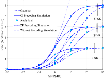
(a) Rate versus SNR with different types of input, when $d_{1}=d_{2}=1m$

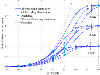
(b) Rate versus SNR with different types of input, when the users are randomly distributed.

Figure 1: Rate versus SNR with different types of input, when $N=2,K=2$.

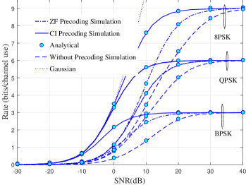
(a) Sum rate versus SNR with different types of input, when $d_{1}=d_{2}=d_{3}=1m$.

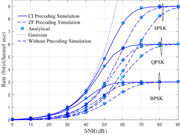
(b) Sum rate versus SNR with different types of input, when the users are randomly distributed.

Figure 2: Rate versus SNR with different types of input, when $N=3,K=3$.

Fig. 1 illustrates the sum-rate for the three transmission schemes, subject to different types of input, BPSK, QPSK and 8PSK, when $N=2$, and $K=2$. Fig. 1a, presents the sum-rate when the distances between the BS and the users are normalized to unit value, .i.e, without the impact of the path-loss. Fig. 1b shows the sum-rate when the users are uniformly distributed inside a circle area with a radius of 80m, and no user is closer to the BS than 10m where the BS is located at the center of this area. The good agreement between the analytical and simulated results confirms the validity of our analysis in the previous sections. From this figure, we have several observations. Firstly, it is evident that the sum rate saturates to the value of, $K\log_{2}M$, past a certain SNR, owing to the finite constellation; the sum rates saturate at 2 bits/s/Hz in BPSK, at 4 bits/s/Hz in QPSK and at 6 bits/s/Hz in 8PSK. In addition, the CI technique always outperforms the ZF and non-precoding techniques for a wide SNR range with an up to 5dB gain in the SNR for a given sum rate. Finally, comparing Fig. 1a and Fig. 1b, one can notice that, in general, increasing the distance always degrades the achievable sum rates. In addition, when the distance between the BS and the users increases the rate saturation occurs at high SNR values, due to larger path-loss. Furthermore, it is worth noting that, the gain attained by CI over the ZF does not depend on the users’ locations.

To capture the influence of number of BS antennas and number of users on the system performance, we present in Fig. 2 the sum-rate for the considered transmission schemes for BPSK, QPSK and 8PSK, when $N=3$, and $K=3$. Comparing the results in this figure with the ones in Fig. 1, it is clear that increasing $N$ and/or $K$ leads to enhance the system performance. In addition, the CI technique always outperforms the ZF technique with an up to 7dB gain in the SNR for a given sum rate. Furthermore, comparing the sum rate achieved in Fig. 2a and Fig. 2b, we can see similar observations as in the case when $N=K=2$.

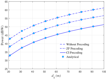
Figure 3: Minimum power transmission versus $d_{k}$ with BPSK input, when $R_{T}=0.5\,\left(\textrm{bits/s/Hz}\right),\,N=2,\textrm{and}K=2$.

In Fig. 3 we plot the minimum power transmission versus a user distance, when $N=2$, $K=2$ and the target data rate, $R_{T}=0.5\textrm{ bits/s/Hz}$ in BPSK scenario. It should be pointed out that the results for the conventional, ZF and CI techniques in this figure are obtained from Section VI. Generally and as anticipated, the CI technique consumes much smaller power transmission than the other two schemes to achieve the same target data rate, and this superiority is almost fixed with the distance.

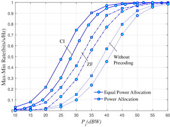
Figure 4: Total max-min rate versus power with BPSK input, when $N=2,\,K=2,\,d_{k}=15\textrm{m}.$.

Moreover, the max-min rate of the considered system versus the total power is shown in Fig. 4. From this figure, it can be clearly noticed that, the rate can be enhanced significantly by using the proposed power allocation algorithm. Furthermore, the CI always has higher sum-rate than ZF and un-precoded techniques.

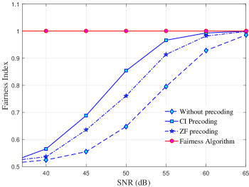
Figure 5: Fairness index versus SNR with BPSK, when $N=\,K=2,\,d_{1}=10\textrm{m},\,d_{2}=90\textrm{m}$.

Finally, Fig. 5 illustrates the Jain’s fairness index versus the SNR. The fairness index is defined as [26], $\frac{\left(\stackrel{{\scriptstyle[}}{{k}}=1]{K}{\sum}R_{k}\right)^{2}}{K\stackrel{{\scriptstyle[}}{{k}}=1]{K}{\sum}R_{k}^{2}}$, the range of Jain’s fairness index is between 0 and 1, where the maximum achieved when users’ rates are equal. It can be observed that, in case equal power allocation transmission, the fairness index increases as the SNR increases, and the CI achieves higher fairness than the other transmission techniques. In addition and as anticipated, the proposed power allocation algorithm performs higher fairness index than equal power allocation transmission scheme.

VIII Conclusions

In this paper we analyzed for the first time the performance of CI precoding technique in MU-MIMO systems with a PSK input alphabet. In light of this, new explicit analytical expressions for the average sum rate are derived for three downlink transmission schemes: 1) without precoding, 2) ZF precoding technique 3) CI precoding technique. In addition, based on the derived sum-rate expressions, the minimum transmission power that performs a target data rate was obtained for each transmission scheme, and then power allocation algorithm has been proposed to provide fairness among the users. The results in this work demonstrated that no matter what the values of the system parameters are, the CI scheme outperforms the other two schemes, and the performance gap between the considered schemes depends essentially on the system parameters. Furthermore, increasing the SNR enhances the sum rate to a certain level, and increasing the distance between the BS and the users has no impact on the gap between the minimum transmission power required for ZF and CI to achieve same target data rate. Finally, it was shown that, the CI can provide higher fairness than ZF technique, and the power allocation algorithm proposed can perform high fairness index.

References

• [1] M. S. John G. Proakis, Digital Communications, Fifth Edition.   McGraw-Hill, NY USA, 2008.
• [2] C. B. P. Howard Huang and S. Venkatesan, MIMO Communication for cellular Networks.   Springer, 2012, 2008.
• [3] Y. Wu, C. Xiao, X. Gao, J. D. Matyjas, and Z. Ding, “Linear precoder design for mimo interference channels with finite-alphabet signaling,” IEEE Transactions on Communications, vol. 61, no. 9, pp. 3766–3780, September 2013.
• [4] A. Salem and K. A. Hamdi, “Wireless power transfer in multi-pair two-way af relaying networks,” IEEE Transactions on Communications, vol. 64, no. 11, pp. 4578–4591, Nov 2016.
• [5] W. Wu, K. Wang, W. Zeng, Z. Ding, and C. Xiao, “Cooperative multi-cell mimo downlink precoding with finite-alphabet inputs,” IEEE Transactions on Communications, vol. 63, no. 3, pp. 766–779, March 2015.
• [6] W. He and C. N. Georghiades, “Computing the capacity of a mimo fading channel under psk signaling,” IEEE Transactions on Information Theory, vol. 51, no. 5, pp. 1794–1803, May 2005.
• [7] C. Xiao, Y. R. Zheng, and Z. Ding, “Globally optimal linear precoders for finite alphabet signals over complex vector gaussian channels,” IEEE Transactions on Signal Processing, vol. 59, no. 7, pp. 3301–3314, July 2011.
• [8] Y. Wu, M. Wang, C. Xiao, Z. Ding, and X. Gao, “Linear precoding for mimo broadcast channels with finite-alphabet constraints,” IEEE Transactions on Wireless Communications, vol. 11, no. 8, pp. 2906–2920, August 2012.
• [9] W. Zeng, C. Xiao, and J. Lu, “A low-complexity design of linear precoding for mimo channels with finite-alphabet inputs,” IEEE Wireless Communications Letters, vol. 1, no. 1, pp. 38–41, February 2012.
• [10] W. Zeng, C. Xiao, M. Wang, and J. Lu, “Linear precoding for finite-alphabet inputs over mimo fading channels with statistical csi,” IEEE Transactions on Signal Processing, vol. 60, no. 6, pp. 3134–3148, June 2012.
• [11] M. Wang, W. Zeng, and C. Xiao, “Linear precoding for mimo multiple access channels with finite discrete inputs,” IEEE Transactions on Wireless Communications, vol. 10, no. 11, pp. 3934–3942, November 2011.
• [12] Y. Wu, C. Xiao, X. Gao, J. D. Matyjas, and Z. Ding, “Linear precoder design for mimo interference channels with finite-alphabet signaling,” IEEE Transactions on Communications, vol. 61, no. 9, pp. 3766–3780, September 2013.
• [13] C. Masouros and E. Alsusa, “Dynamic linear precoding for the exploitation of known interference in mimo broadcast systems,” IEEE Transactions on Wireless Communications, vol. 8, no. 3, pp. 1396–1404, March 2009.
• [14] C. Masouros, M. Sellathurai, and T. Ratnarajah, “Vector perturbation based on symbol scaling for limited feedback miso downlinks,” IEEE Transactions on Signal Processing, vol. 62, no. 3, pp. 562–571, Feb 2014.
• [15] C. Masouros and G. Zheng, “Exploiting known interference as green signal power for downlink beamforming optimization,” IEEE Transactions on Signal Processing, vol. 63, no. 14, pp. 3628–3640, July 2015.
• [16] S. Timotheou, G. Zheng, C. Masouros, and I. Krikidis, “Exploiting constructive interference for simultaneous wireless information and power transfer in multiuser downlink systems,” IEEE Journal on Selected Areas in Communications, vol. 34, no. 5, pp. 1772–1784, May 2016.
• [17] M. R. A. Khandaker, C. Masouros, and K. K. Wong, “Constructive interference based secure precoding: A new dimension in physical layer security,” IEEE Transactions on Information Forensics and Security, vol. 13, no. 9, pp. 2256–2268, Sept 2018.
• [18] P. V. Amadori and C. Masouros, “Large scale antenna selection and precoding for interference exploitation,” IEEE Transactions on Communications, vol. 65, no. 10, pp. 4529–4542, Oct 2017.
• [19] A. Li and C. Masouros, “Interference exploitation precoding made practical: Optimal closed-form solutions for psk modulations,” IEEE Transactions on Wireless Communications, pp. 1–1, 2018.
• [20] M. Abramowitz and I. A. Stegun, Handbook of Mathematical Functions With Formulas, Graphs, and Mathematical Tabl, Washington,D.C.: U.S. Dept. Commerce, 1972.
• [21] R. Zhang, L. Yang, and L. Hanzo, “Error probability and capacity analysis of generalised pre-coding aided spatial modulation,” IEEE Transactions on Wireless Communications, vol. 14, no. 1, pp. 364–375, Jan 2015.
• [22] D. Lee, “Performance analysis of zero-forcing-precoded scheduling system with adaptive modulation for multiuser-multiple input multiple output transmission,” IET Communications, vol. 9, no. 16, pp. 2007–2012, 2015.
• [23] C. Masouros, T. Ratnarajah, M. Sellathurai, C. B. Papadias, and A. K. Shukla, “Known interference in the cellular downlink: a performance limiting factor or a source of green signal power?” IEEE Communications Magazine, vol. 51, no. 10, pp. 162–171, October 2013.
• [24] G. Zheng, I. Krikidis, C. Masouros, S. Timotheou, D. A. Toumpakaris, and Z. Ding, “Rethinking the role of interference in wireless networks,” IEEE Communications Magazine, vol. 52, no. 11, pp. 152–158, Nov 2014.
• [25] R. J. Muirhead, Aspects of Multivariate Statistical Theory, 1982.
• [26] H. B. Jung and D. K. Kim, “Power control of femtocells based on max-min fairness in heterogeneous networks,” IEEE Communications Letters, vol. 17, no. 7, pp. 1372–1375, July 2013.