Event-chain Monte Carlo with factor fields

Abstract

We study the dynamics of one-dimensional (1D) interacting particles simulated with the event-chain Monte Carlo algorithm (ECMC). We argue that previous versions of the algorithm suffer from a mismatch in the factor potential between different particle pairs (factors) and show that in 1D models, this mismatch is overcome by factor fields. ECMC with factor fields is motivated, in 1D, for the harmonic model, and validated for the Lennard-Jones model as well as for hard spheres. In 1D particle systems with short-range interactions, autocorrelation times generally scale with the second power of the system size for reversible Monte Carlo dynamics, and with its first power for regular ECMC and for molecular-dynamics. We show, using numerical simulations, that they grow only with the square root of the systems size for ECMC with factor fields. Mixing times, which bound the time to reach equilibrium from an arbitrary initial configuration, grow with the first power of the system size.

I Introduction

The dynamics of physical systems plays an important role in numerous fields of science. The study of dynamics aims at elucidating equilibrium and non-equilibrium phenomena, including correlation functions, coarsening dynamics after a quench, and manifestly non-equilibrium phenomena such as turbulence. In computational statistical physics, Markov chain Monte Carlo (MCMC) Metropolis1953 ; Levin2008 ; SMAC and molecular-dynamics (MD) algorithms Alder1957 are often employed to generate equilibrated samples and to determine thermodynamic averages and correlations. The non-equilibrium aspect then consists in characterizing the approach to equilibrium from an arbitrary, atypical, initial condition. This is quantified by the mixing time Levin2008 , an important figure of merit for MCMC. The other important time scale characteristic of a physical system is the autocorrelation times of the underlying Markov process given by the inverse gap of the transition matrix.

In reversible Markov chains (as used in the vast majority of MCMC algorithms), the requirement that the long-time steady state corresponds to thermodynamic equilibrium is expressed through the detailed-balance condition, which assures that all the net probability flows vanish in equilibrium. In recent years, however, irreversible Markov chains have been found to show considerable promise Turitsyn2011 ; SakaiIsing2013 ; SakaiEigenvaluePRE2016 ; Bierkens2018 . They feature a steady state with non-vanishing net probability flows if a weaker global-balance condition is satisfied. Global balance corresponds to an incompressibility condition in configuration space: the steady-state flows into each configuration sum to the flows out of it.

An example of an irreversible Markov chain is the event-chain algorithm (ECMC) Bernard2009 ; Michel2014JCP . This algorithm has been successfully applied to many problems from hard-sphere and soft-sphere melting Bernard2011 ; Engel2013 ; Kapfer2015PRL to spin models MichelMayerKrauth2015 ; Nishikawa2015 and quantum-field theory HasenbuschSchaefer2018 . In this paper, we study the relaxation times of ECMC in one-dimensional (1D) models of $N$ particles with local interactions KapferKrauth2017 ; Lei2018b . We analyze in detail the relaxation of both Lennard-Jones and hard-sphere models, study the statistical properties of ECMC trajectories and show how to greatly accelerate known algorithms by the introduction of a “factor field”, which compensates the system pressure, $P$, without influencing physical properties.

I.1 Characteristic times of Markov chains

Irreversible MCMC algorithms can be faster than their reversible counterparts. A particularly interesting case is the 1D hard-sphere model of $N$ spheres (rods). For this model, the local heat-bath algorithm mixes in $\mathcal{O}\left(N^{3}\log{N}\right)$ moves RandallWinklerInterval2005 on an interval with fixed boundary conditions. The mixing time for the same model with periodic boundary conditions is between $\mathcal{O}\left(N^{3}\right)$ and $\mathcal{O}\left(N^{3}\log{N}\right)$ RandallWinklerCircle2005 : Simulations favor the latter KapferKrauth2017 . The reversible Metropolis algorithm has a similar mixing behavior. Various local irreversible Markov chains mix in $\mathcal{O}\left(N^{5/2}\right)$ moves (forward Metropolis algorithm KapferKrauth2017 ), in $\mathcal{O}\left(N^{2}\log{N}\right)$ steps (lifted forward Metropolis algorithm and ECMC KapferKrauth2017 ; Lei2018b ) and even $\mathcal{O}\left(N^{2}\right)$ single moves with a re-labeling ECMC Lei2018b .

The lifted forward Metropolis algorithm in continuous space with infinitesimal movements constitutes ECMC. For hard spheres, it is deterministic without restarts, but then mixes in $\mathcal{O}\left(N^{2}\log N\right)$ steps at randomized stopping times Lei2018b . Although ECMC is irreversible under a transformation of the time $t\mapsto-t$, under the combined transformation of times and positions $(t,x)\mapsto(-t,-x)$, the dynamics runs backwards in time. The irreducibility of the lifted forward Metropolis algorithm can be shown using this time-reversal property. It may also explain why ECMC is typically as fast as MD.

Previous work has also explored the autocorrelation times (rather than the mixing times) under ECMC dynamics in the $D$-dimensional harmonic-solid model, of which the equilibrium properties can also be obtained exactly (see Lei2018 ). In 1D, the dynamic exponent of the autocorrelations under ECMC dynamics takes the strikingly low value of $z=1/2$, corresponding to an equilibrium autocorrelation time involving $\mathcal{O}(N^{3/2})$ moves or $\tau\sim\mathcal{O}(N^{1/2})$ sweeps. This is $N^{1/2}$ times smaller (faster) than the best autocorrelation time found in the hard-sphere system.

The present paper starts from the similarity between the dynamics of the 1D harmonic-solid model and that of the Lennard-Jones model at low temperature $T$. We generalize this favorable scaling of the harmonic model to all $T$ in the Lennard-Jones model as well as the hard-sphere model. We expect that this concept can also be generalized for higher-dimensional models Faulkner2018 ; MaggsMultiscale2006 .

I.2 1D particle systems, algorithms

We consider a 1D system of $N$ particles $i\in\{1,\ldots,N\}$ with $x_{i}<x_{i+1}$ on an interval of length $L$ with periodic boundary conditions in $N$ and in $L$. In the reversible local Metropolis algorithm, at each iteration, a randomly chosen particle $i$ is proposed to move as $x_{i}\to x_{i}+\text{ran}[-\epsilon,\epsilon]$, where ran is a random number uniformly distributed between $-\epsilon$ and $\epsilon$. For hard spheres, the move is accepted if the new sphere position does not lead to overlaps with spheres $i-1$ and $i+1$, and in addition does not induce a change of the ordering. In the presence of a potential $U$, the move is accepted with probability $\min(1,\exp(-\Delta U/T))$, where $\Delta U$ is the change in potential for the proposed move. The amplitude $\epsilon$ is chosen to maximize the speed of the method. In the heat-bath algorithm the distribution of the particle $i$ is fully resampled in the potential of its neighbors at each time step.

ECMC, for one-dimensional hard spheres Bernard2009 ; KapferKrauth2017 , consists in moving spheres in a chain-like manner. Up to a restart time, sphere $i$ moves with unit velocity until it collides with sphere $i+1$, at which moment it stops, and sphere $i+1$ moves forward. For each of the subsequent “chains” (the displacements between restarts), the starting sphere is randomly chosen, and the length of the chain (the time until the next restart) is sampled from a distribution on the length scale $L$. For a more general interaction potential, ECMC breaks up the total system potential up into separate “factor potentials”, each of which is treated independently Michel2014JCP ; Peters_2012 . A factor potential provides for a randomized stopping time. For a given move involving particle $i$, the smallest stopping time of all factors provides the next event time. The next particle to move is determined through a lifting scheme Harland2017 ; Faulkner2018 from the factor triggering the event. With potentials more general than hard spheres, restarts are no longer required to ensure irreducibility of ECMC.

In ECMC, path statistics in equilibrium and pressure $P$ are linked by

$$P/T\propto\frac{1}{t}\left\langle x_{i(t)}-x_{i(0)}\right\rangle,$$ (1)

where $x_{i}(t)$ is the position of the particle that is active at time $t$ (Michel2014JCP, , eq.(20)). Eq. (1) holds for all time intervals $t$. It is very convenient as an unbiased estimator of the pressure, and has been much used Kapfer2015PRL . The factor fields of the present paper will allow us to exactly compensate the pressure without affecting the physical properties of the system, and lead to greatly accelerated ECMC methods.

In many-particle simulations, MD algorithms generally feature smaller relaxation time scales than MCMC methods. In essence this is because momentum conservation (present in MD, but absent in MCMC) allows for faster transport of inhomogeneities in the velocity and position fields (AlderWainwrightAutocorrelation1970 ; WittmerPolinska2011 ). In our comparisons with ECMC, MD simulations are performed using the leapfrog or Verlet algorithm coupled to a Langevin thermostat for the velocity. The integration time step $\delta t$ is adjusted by finding the stability limit of the integrator, then reducing $\delta t$ by an order of magnitude. Inverse error analysis shows that the effective Hamiltonian is close to that of the original model, with a systematic shift of $O(\delta t^{2})$ in the effective Hamiltonian Hairer2006 . We choose the strength of coupling to the Langevin thermostat so that the longest wavelength mode is close to critically damped.

We concentrate our measurements on the dynamics of the structure factor of the lowest Fourier coefficient

$$S({q})=\frac{1}{N}\left|\sum_{j=1}^{N}\mathrm{e}^{i{q}\cdot x_{j}}\right|^{2},$$ (2)

with $q=2\pi/L$, which is sensitive to large-scale motion of particles. The integrated autocorrelation times $\tau$ of $S(\frac{2\pi}{L})$ are measured in “sweeps”, that is, a constant time interval for all $N$ particles in MD, $N$ attempted displacements in MCMC, or $N$ events in ECMC (in comparing the methods, we compensate for the different implementation speeds of a sweep in MD, MCMC, ECMC). We use the blocking method error to quantify the algorithm speed.

I.3 ECMC for harmonic interactions

We first consider a harmonic potential with a minimum at a separation $b$ between neighboring particles:

$$U_{\text{harm}}(x_{i+1}-x_{i};b)=\frac{k}{2}\left[(x_{i+1}-x_{i})-b\right]^{2},$$ (3)

where periodic boundary conditions for the particle separation $x_{i+1}-x_{i}$ are taken. They are also implied for the particle indices. The total potential of the system of a fixed length $L$ is

$$U_{\text{harm}}(\{x_{i}\};b)= \frac{k}{2}\sum_{i=1}^{N}{(x_{i+1}-x_{i}-b)}^{2}$$ (4)

$$= U_{\text{harm}}(\{x_{i}\};0)-kbL+\frac{1}{2}Nkb^{2},$$ (5)

where periodic boundary conditions in $N$ and $L$ are again understood. Because of the periodic boundary conditions, the choice of the equilibrium separation $b$ simply shifts the ground-state potential, without changing the stationary distribution and equilibrium correlations. Nevertheless, the ground-state potential is dependent on $L$ and it determines some thermodynamic properties, such as the pressure:

$$P_{\text{harm}}(b)=k(b-L/N).$$ (6)

The system with $b=L/N$ satisfies $P_{\text{harm}}=0$.

In a periodic system, MD and the reversible Metropolis algorithm are strictly independent of $b$, as they only rely on the forces (identical derivatives of eqs (4) and (5) with respect to the $x_{i}$) or potential differences between configurations. However, the explicit form of the pairwise interaction influences the ECMC dynamics, as the factor potentials are treated independently. One such factor potential may thus contain the single term $U_{\text{harm}}(x_{i+1}-x_{i};b)$ with its explicit dependence on $b$. In the following we consider such factors between all neighboring pairs of particles. For $b=0$, the harmonic interactions on particle $i$ from its neighbors is attractive if $x_{i-1}<x_{i}<x_{i+1}$. It implies that for an active particle $i$ with a positive displacement, the particle $i-1$ is likely to trigger the next event in ECMC (and to be the next active particle) (see Fig. 1a). The displacement $\delta x$ per event is:

$$\delta x\sim\frac{T}{k(L/N-b)},\;\text{if }T\ll\frac{k}{2}{(L/N-b)}^{2}.$$ (7)

As $b$ increases, the triggering probability is less biased and the displacement gets larger, and eventually reaches the maximum:

$$\delta x\sim\sqrt{\frac{2T}{k}},\;\text{when }b=L/N,$$ (8)

with symmetric triggering probabilities in both directions (see Fig. 1c).

At low $T$, the displacement per event in eq. (7) is much smaller than that in eq. (8). We expect that the case $b=L/N$ leads to larger amplitude movements of the active particle $i$, at the same time the transfer of activity is equally often toward $i+1$ and toward $i-1$, and characterizes the detailed ECMC dynamics. The case $b=L/N$ indeed gives rise to the exceptionally fast dynamics, characterized by $z=1/2$ Lei2018 . The aim of the present paper is to generalize this fast relaxation to arbitrary potentials.

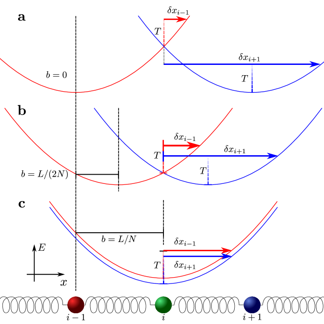
Figure 1: ECMC dynamics in the harmonic model. Particle $i$ is active, and the red and blue curves indicate the interactions with particles $i-1$ and $i+1$, respectively. The proposed moves are indicated by solid colored arrows, with respect to the temperature $T$ (vertical dashed lines). a: For $b=L/N$, the interractions with particles $i-1$ and $i+1$ overlap. b: For $b=L/(2N)$, the potential with $i-1$ proposes a smaller displacement than $i+1$. Particle $i-1$ is more likely to be activated. c: For $b=0$, the moves proposed by $i-1$ and by $i+1$ are balanced.

II Linear Lennard-Jones model with ECMC

We study now the Lennard-Jones potential

$$U_{\text{LJ}}(r)=\frac{1}{r^{12}}-\frac{1}{r^{6}},$$ (9)

where $r=x_{i+1}-x_{i}$, with periodic booundary conditions. The minimum is $U_{\text{LJ}}(r_{\min})=-1/4$ for $r_{\min}=2^{1/6}$, which sets a typical potential scale of the system $\epsilon=|U_{\text{LJ}}(r_{\min})|$. In previous work Faulkner2018 we proposed multiple factor sets within ECMC. Here we take into consideration two distinct factor sets $\mathcal{M}_{LJ}$ and $\mathcal{M}_{6+12}$: the former groups the terms $1/r^{6}$ and $1/r^{12}$ into a single Lennard-Jones factor, while the latter treats them separately as two factors which independently trigger events.

As the particles always move in the positive direction ($x_{i}$ is always increasing), the active particle $i$, with the factor set $\mathcal{M}_{6+12}$, will either trigger the particle $(i+1)$ by the repulsive contribution $1/r^{12}$ or the particle $(i-1)$ by the attractive contribution $1/r^{6}$. The factor set $\mathcal{M}_{LJ}$ can lead to a trigger from $(i+1)$ or $(i-1)$ since the Lennard-Jones interaction has both increasing and decreasing branches.

In the following, we will show that the large-scale dynamics of ECMC are very sensitive to the choice of factor sets, even if all choices lead to the same equilibrium state. Good choices are crucial in the creation of efficient algorithms.

II.1 Simulations of 1D Lennard-Jones models

We simulate a slightly compressed ($P>0$) linear Lennard-Jones model with periodic boundary conditions with average separation between particles equal to $\Delta=1.06<r_{\min}$ and use the reversible local Metropolis MCMC method, MD, as well as ECMC with the factor set $\mathcal{M}_{LJ}$ (see Fig. 2a). Metropolis MCMC is asymptotically the slowest method for $N\to\infty$: the autocorrelation time (measured in sweeps) increases as $N^{z}$ with $z=2$ characteristic of the diffusion of density fluctuations. MD is better behaved, due to the propagative compressional waves which more efficiently sample long-wavelength modes. MD is however disadvantaged by the necessity of using a small integration time step $\delta t$ to stably explore the dynamics. The result from ECMC is very favorable, we see a low dynamic exponent ($z=1$) combined with a small prefactor in the scaling: the algorithm makes a large leap (without systematic errors) for each iteration.

However, ECMC can also be less efficient than MD, in certain implementations (see Fig. 2b). Here we use the factor set $\mathcal{M}_{6+12}$, at low $T$. Here an analogous phenomenon occurs to that displayed in Fig. 1, in a form which is amplified by the splitting of the $1/r^{6}$ and $1/r^{12}$ contributions to the potential. The algorithm advances with the use of steps which are too small to efficiently explore the local environment. This slowdown of ECMC at low $T$ was pointed out previously Hu2018 . We now study analytically the Lennard-Jones interaction in eq. (9) at low $T$, and make contact with the harmonic model in order to eliminate this slowdown.

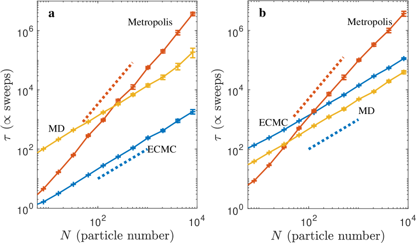
Figure 2: Equilibrium autocorrelation times $\tau$ vs. system size $N$, for the 1D periodic Lennard-Jones model. Reversible local Markov-chain dynamics, ECMC with restarts and MD. a: $T/\epsilon=10$, combined factors, $\mathcal{M}_{LJ}$. b: $T/\epsilon=0.1$, separate factors, $\mathcal{M}_{6+12}$. Scalings $\tau\sim N$ and $\tau\sim N^{2}$ are indicated with dotted lines.

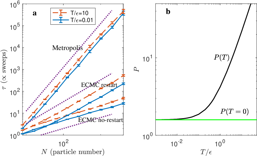
Figure 3: Equilibrium autocorrelation timess $\tau$ vs. system size $N$, for the 1D periodic Lennard-Jones system with factor fields. a: Reversible local Metropolis dynamics and ECMC with and without restarts, at high $T$, $T/\epsilon=10$ and low $T$, $T/\epsilon=0.01$. Scalings $\tau\sim N^{1/2}$, $\tau\sim N$, and $\tau\sim N^{2}$ are indicated with dotted lines. b: Pressure $P(T)$ and its $T\to 0$ limit (see eq. (13)).

A straightforward expansion of the potential $U_{\text{LJ}}(r)$ of eq. (9) to second order around a generic position $r=\Delta$ yields

$$U_{\text{LJ}}(r) =U_{\text{LJ}}(\Delta)-h_{\text{LJ}}(\Delta)(r-\Delta)$$ (10)

$$+\frac{1}{2}k_{\text{LJ}}(\Delta){(r-\Delta)}^{2}+\ldots.$$ (11)

This validates the (obvious) fact that the 1D Lennard-Jones model, in the limit $T\to 0$, is described by a harmonic model with, in analogy to eq. (5), a “stiffness”

$$\frac{1}{2}k_{\text{LJ}}(\Delta)=\left(\frac{78}{\Delta^{14}}-\frac{21}{\Delta^{8}}\right)$$ (12)

and a linear coefficient

$$h_{\text{LJ}}(\Delta)=-6(-2+\Delta^{6})/\Delta^{13}.$$ (13)

Summed over the $N$ pairs $(i,i+1)$ (with periodic boundary conditions), the constant ($U_{\text{LJ}}(\Delta)$) and the first-order term in eq. (11) are without incidence on the constant-volume thermodynamics and the stationary distribution.

Analogously to eq. (5), we may add a temperature-dependent factor-field interaction

$$U^{\text{fact}}_{\text{LJ}}=h^{\text{fact}}_{\text{LJ}}(T)\sum_{i=1}^{N}\left(x_{i+1}-x_{i}\right)$$ (14)

to the total Lennard-Jones potential $\sum_{i}U_{\text{LJ}}(x_{i+1}-x_{i})$. The model defined by $U_{\text{LJ}}+U^{\text{fact}}_{\text{LJ}}$ differs from the model given by $U_{\text{LJ}}$ alone (in the presence of periodic boundary conditions), as the two have different pressures. Nevertheless, the samples obtained from the two associated Boltzmann distributions are the same, and therefore also all probability distributions and correlation functions at constant $L$. We choose a factor field to exactly compensate the linear term in the interaction in the limit $T\to 0$:

$$h^{\text{fact}}_{\text{LJ}}(T)=h_{\text{LJ}}(\Delta)\quad\text{(for small $T$)}.$$ (15)

This clearly eliminates the inefficiencies of ECMC at low temperatures. In the model defined by eq. (15), the pressure $P$ vanishes as $T\to 0$. Because of the connection between the pressure and the path statistics expressed in eq. (1), the ECMC trajectories are then without a drift term, and the expected displacement vanishes. As we now confirm numerically, we can speed up ECMC at arbitrary $T$ by adopting a factor potential that exactly compensates for $P$.

We start by performing a set of short simulations to measure $P$ from eq. (1) (see Fig. 3b). The function $P(T)$, thus obtained, recovers the $T\to 0$ limit. We then fix the value of the factor field in longer simulations to characterize the dynamics (see Fig. 3a). Indeed, both at low and at high $T$, ECMC remains efficient, and the dynamical exponent $z=1/2$ corresponds to the harmonic model for $b=L/N$. This was tested for temperatures as high as $T/\epsilon=10$ where the interactions for Lennard-Jones particles are dominated by the short-ranged repulsive core. The ansatz $h^{\text{fact}}=P$ for the factor field thus holds at temperatures at which the harmonic approximation of the potential no longer applies. Maximum efficiency is found for ECMC without restarts only: restarting the chain after $\sim N$ events leads to a larger dynamic exponent.

For the Lennard-Jones system, ECMC with factor fields requires finding roots to the equations

$$\frac{1}{r^{12}}-\frac{1}{r^{6}}\pm Pr=\Delta U.$$ (16)

We use the iterative Halley method Halley , a higher-order generalization of Newton’s method. It has the advantage of stability when starting an iteration near a stationary point of the function eq. (16). We start the iteration with a guess obtained with one of two methods. For small $\Delta E$ we make a harmonic approximation to the left-hand side of eq. (16). For large $\Delta E$, the starting point is approximated as a root to the equation $1/r^{12}=\Delta E$. The iteration converges to machine precision within three iterations. The relative speeds shown in Fig. 3a account for this slow, iterative step through an appropriate proportionality factor for each algorithm. Alternatives to root finding may including thinning methods (as used in the cell-veto algorithm KapferKrauth2016 ) which compare rates derived from eq. (16) to an analytically tractable bound.

II.2 Extensions: Alternative factor sets

ECMC allows for many other choices for factors and also for lifting schemes. We may generalize the factor field method to the $\mathcal{M}_{6+12}$ factor set by introducing one factor field each for $1/r^{6}$ and for $1/r^{12}$ interactions (checking the convergence of the method for multiple correlation functions), but we did not explore fully the optimal choice of the two factor fields. We also studied factor sets which contain all the interactions of the model. This scheme is particularly interesting because the active particle $i$ simultaneously explores the potential due to both $i-1$ and $i+1$, without the need for an explicit factor field. Again, this scheme uses an iterative solver. The full system factors also require a more sophisticated lifting scheme – generalizations of the “inside first” and “outside first” methods  Faulkner2018 . Particles with positive factor derivatives and particles with negative factor derivative are aligned in index order (see for instance (Faulkner2018, , Fig. 10)). The lifting dynamics corresponds to the alignment of factors vertically. In such schemes, factors contain $\mathcal{O}\left(N\right)$ terms. Efficient alignment of the lifting diagram requires the use of a tree structure for bookkeeping with an effort $\mathcal{O}\left(\log\!\,(N)\right)$. We found this method however to be less efficient than the factor field, and so do not report further on speed measurements.

III Factor fields for 1D hard spheres

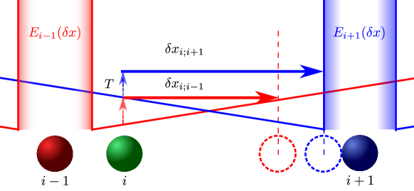
Figure 4: ECMC dynamics with factor fields (indicated by inclined straight lines) for 1D hard spheres. The moves of the active sphere $i$ proposed by the factors with $i+1$ and $i-1$ are indicated by horizontal arrows and dashed sphere positions. In the optimal dynamics, the slopes of the factor fields equal $\pm P$ in eq. (17).

To illustrate the generality of factor fields, we now consider their application to the 1D hard-sphere model, where the potential can no longer be expanded as a power series (as in eq. (11)). Nevertheless, the model has a well-defined pressure, that is computed from the partition function $Z={(L-N\sigma)}^{N}$. This gives for the free energy, at temperature $T$, $F=-T\log Z=-NT\log L_{\text{free}}$, with $L_{\text{free}}=L-N\sigma$ and therefore Tonks1936

$$P=\frac{NT}{L_{\text{free}}}.$$ (17)

III.1 Implementation, autocorrelation times

The implementation of ECMC with factor fields for hard spheres does not require numerical root finding: an active particle $i$, moving to the right, generates two possible events, a hard-sphere collision with the particle $i+1$ or else a trigger due to the factor field of particle $i-1$ (see Fig. 4). The latter path length is sampled from an exponential distribution

$$\rho(x)=\frac{P}{T}\mathrm{e}^{-xP/T}.$$ (18)

The smaller of the two proposed displacements yields the next event, and it defines the lifting, as the new active particle is the one that has triggered the event. Irreducibility is guaranteed in the dynamics with an infinite event chain, and restarts are no longer needed, unlike for hard-sphere ECMC without the factor field.

We study the autocorrelation time in sweeps (see Fig. 5a) and compare with the reversible local Metropolis algorithm as well as ECMC without a factor field. Again, we note the acceleration brought by the addition of a factor field with a dynamic exponent $z=1/2$, just as for the linear Lennard-Jones and the harmonic models. Non-optimal factor fields slow down the dynamics of the longest wavelength modes, an effect which becomes stronger for larger $N$ (see Fig. 5b).

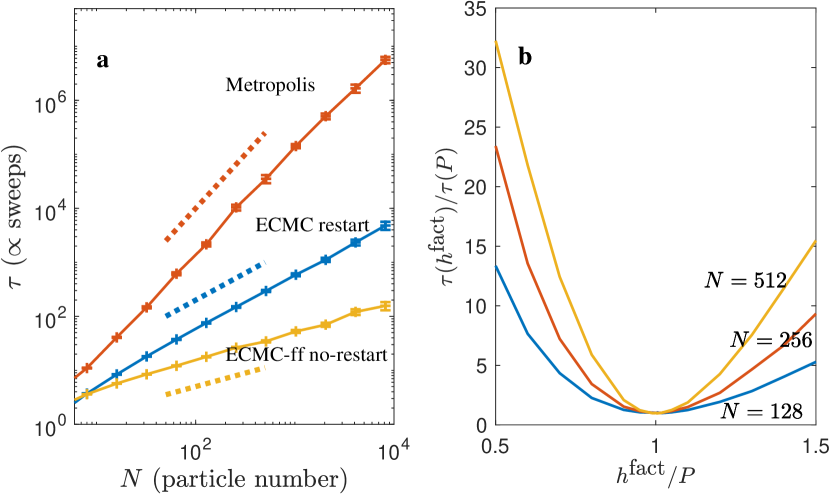
Figure 5: Autocorrelation time $\tau$ (in sweeps) for 1D hard spheres. a: Reversible local Metropolis MCMC, ECMC (with restarts) and without factor field and ECMC (without restarts) with optimal factor field, $h^{\text{fact}}$. Scalings $\tau\sim N^{1/2}$, $\tau\sim N$, and $\tau\sim N^{2}$ are indicated with dotted lines. b: $\tau$ from ECMC vs. factor field (ECMC, without restarts).

III.2 Evaluation of mixing times

We have so far considered the equilibrium autocorrelation time, which is only one of the two relevant measures for the speed of an algorithm; it measures the time to move from one configuration (taken in equilibrium) to another independent one. The mixing time, in contrast, considers the time it takes to reach a first equilibrium configuration from an arbitrary non-equilibrium state. The scaling with $N$ of the equilibrium autocorrelation time and of the mixing time differs for many MCMC algorithms in 1D particle systems (see Levin2008 for a mathematical discussion of mixing times and equilibrium autocorrelation times, and Lei2018b for a discussion in the context of ECMC.)

To determine the mixing time for the hard-sphere model with factor fields, we use a discretized version of the smallest Fourier coefficient of the structure factor in eq. (2), namely the variance $\text{var}(w)$ of the “half-system distance”

$$w=x_{i+N/2}-x_{i}-N\sigma/2$$ (19)

from a compact initial configuration KapferKrauth2017 where $\text{var}(w)\propto N^{2}$ to the (exactly known) equilibrium value, which is $\propto N$. Tracking the variance signals a mixing time very close to $N$ sweeps, a value that we conjecture to be exact (see Fig. 6). This is a faster scaling than the $\mathcal{O}\left(N\log N\right)$ sweep mixing-time behavior of ECMC with restarts (without factor field) Lei2018b .

Relaxation occurs in the following manner from a compact configuration: First, the active particle is driven to the right end of the system which over-relaxes (see Fig. 6). This drives the activity back into the bulk, to the boundary with the compact interior. A series of cycles of increasing amplitude relaxes the end of the system with penetration into the compact region following a law in $\sqrt{t}$. We note that the mixing time is longer than the equilibrium autocorrelation time (see the discussion in Section IV).

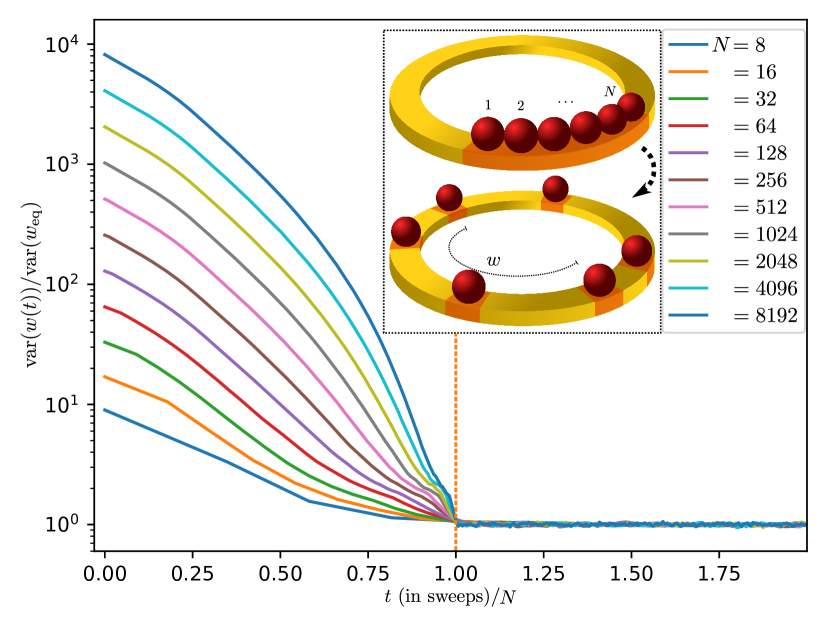
Figure 6: Variance of the half-system distance $w$ (see eq. (19)) vs. time for various $N$ (hard-sphere model with factor fields (without restarts)). The observable relaxes to its equilibrium value at the mixing time $(1.000\pm 0.005)\times N$ sweeps for the hard-sphere model with factor fields (without restarts).

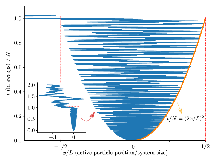
Figure 7: Position $x_{i}$ of the active sphere $i$ vs. time $t$ ($N=4096,\sigma=L/(2N)$). At $t=0$, the interval $[-L/2,0]$ is close packed, the interval $[0,L/2]$ is empty. The physical extent expands through oscillations, growing as $\sqrt{t}$, and reaches $[x_{1},x_{N}]\simeq L$ at $t\simeq N$. The inset illustrates the position of $x_{i}$ (without periodic wrapping) on a larger time interval.

IV Active-particle dynamics

The choice of factor fields, even if it is without incidence on spatial correlation functions and thermodynamic properties at constant $L$, strongly influences the ECMC dynamics. In this section, we consider the large-scale motion of the particle $i(t)$ that is active at time $t$, in order to probe how the exponent $z=1/2$ arises from the local active-particle dynamics. It is convenient to take into consideration discrete “event times” $s=0,1,2,\dots$, rather than the continuous time $t$ of the Markov process. Because of the ordering of indices, we have $i(s+1)=i\pm 1$, with “event steps” $u(s)$ as $i(s+1)=i(s)+u(s)$ and $u(s)\in\{-1,1\}$. It follows from eq. (1) that $\left\langle u\right\rangle>0$ and $\left\langle u\right\rangle<0$ for $P>0$ and $P<0$, respectively, which means that the ECMC trajectory is described by a forward drift (for $P>0$) or a backward drift (for $P<0$). With a factor field equal to $P$, the drift terms vanish, and ECMC trajectories feature positive and negative event steps (liftings $i(s+1)=i(s)+1$ and $i(s+1)=i(s)-1$) with equal probabilities Anomalous2017 . To better characterize the time series $u(s)$ in this case, for both hard spheres and Lennard-Jones particles, we compute the event-step autocorrelation $\left\langle u(0)u(s)\right\rangle$ (see Fig. 8). We find that for large $N$, the autocorrelation decays as a power law:

$$\left\langle u(0)u(s)\right\rangle\sim s^{-\gamma}.$$ (20)

(This scaling applies on times shorter than those required to explore the whole system. On longer time scales the correlation in eq. (20) decays exponentially.)

The active particle at event time $s$ (without periodic wrapping) is given by

$$i(s)=i(s=0)+\sum_{s^{\prime}=1}^{s}u(s^{\prime}).$$ (21)

We now follow a trajectory which starts with $i(s=0)=0$. For vanishing long-range correlations in the event steps $u(s)$, the motion of the activity, characterized by the second moment of $i(s)$, would be diffusive ($\left\langle i^{2}(s)\right\rangle\sim s$. Rather, we find for large $s$, using eq. (20) with $\gamma<1$:

$$\left\langle i^{2}(s)\right\rangle=\sum_{s^{\prime}=1}^{s}\sum_{s^{\prime\prime}=1}^{s}\left\langle u(s^{\prime})u(s^{\prime\prime})\right\rangle\sim s^{2-\gamma}.$$ (22)

The position of the active particle is thus characterized by super-diffusive behavior. The observed value $\gamma=2/3$ (see Fig. 8) implies

$$\left\langle i^{2}\right\rangle\sim s^{4/3}\quad\text{or}\quad|i|\sim s^{2/3}.$$ (23)

The dynamics of the active particle has long-time memory for $N\to\infty$. The trajectories contain long runs separated by changes of the direction of motion, so that the average motion is undirected, as required by eq. (1).

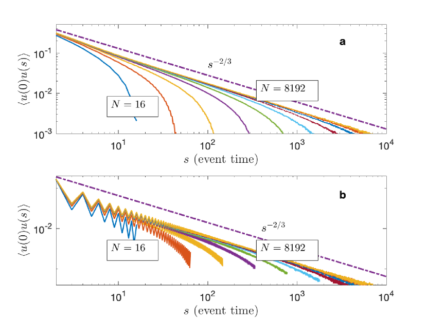
Figure 8: Equilibrium autocorrelation of event steps $u\in\{-1,1\}$ with event time $s$ for ECMC with factor field (no restarts). a: 1D Lennard-Jones model shows monotonic decay. b: 1D hard spheres display oscillatory behavior with a power-law envelope. The scaling $\left\langle u(0)u(s)\right\rangle\sim s^{-2/3}$ is indicated with dotted lines (see eq. (20)).

IV.1 Scaling for the active-particle dynamics

The discrete event time $s=0,1,2,\dots$ grows with the time $t$ of the Markov process (that we measure in sweeps) as $s\propto Nt$. The same argument applies to the autocorrelation event time, in events, and the autocorrelation time $\tau$, in sweeps, $s_{\text{auto}}\propto N\tau(N)$. The super-diffusive motion constrains the dynamic exponent $z$ which relates complexity to system size:

$$s_{\text{auto}}\sim N^{(1+z)}.$$ (24)

A configuration can decorrelate from its previous history only if the super-diffusive walk visits each sphere at least once. Thus we require:

$$|i(\tau)|\sim{s_{\text{auto}}}^{1-\gamma/2}\sim N^{(1+z)(1-\gamma/2)}\geq N,$$ (25)

implying that $z\geq\gamma/(2-\gamma)$. If we take $\gamma=2/3$, we find $z\geq 1/2$ compatible with the autocorrelation scaling reported previously for the harmonic model Lei2018b , and also compatible with the data in Figs 2 and 5.

A supplementary physical hypothesis of perfect local equilibration during the ECMC motion leads to a definite prediction for $\gamma$: the equalibrium fluctuations in particle separation in a system section of length $|i|$ increase as

$$\Delta x_{p}\sim|i|^{1/2}.$$ (26)

After $s$ events the active label visits particles in a volume $|i|\sim s^{1-\gamma/2}$, so that on average each particle moves

$$\Delta x_{\gamma}=\frac{s}{|i|}\sim s^{\gamma/2}\sim|i|^{\gamma/(2-\gamma)}$$ (27)

times. If we assume that the motion of the particles is comparable to that required to resample the internal states of the section of length $|i|$ we find $\Delta x_{p}\sim\Delta x_{\gamma}$ so that $\gamma=2/3$, and $z=1/2$.

For this mechanism to work, the correlated random motion of the active particle must behave in a special way: both the mean and the standard deviation of the distribution of $\Delta x_{\gamma}$ must have identical scaling with $s$. (If only the mean increases the spheres will be displaced uniformly without re-equilibrating the internal degrees of freedom.)

IV.2 Active-particle return probabilities

The distribution of eq. (27)) allows for a rapid decay of autocorrelation functions. We consider the dynamics of a particle which is active at time $s=0$. This particle can only move forward a large distance if the active label returns to it frequently, that is, if for many times $s$, one has $i(s)=i(s=0)$. We thus study in greater detail the returns to the origin of the active label, in the presence of factor fields.

We generate an equilibrated configuration of the Lennard-Jones system and from the signal $i(s)$ calculate the distribution of the number $n$ of returns to the origin within $s$ events (see Fig. 9). For Brownian walks of length $s$, $n$ is related to the “local time” feller-vol-1 ; localtime , and the local-time distribution $p(n,s)$ is half-gaussian defined for $n>0$. In ECMC, the probability $p(n,s)$ of returns of the active-particle label to the origin (which gives the number of forward steps) is also maximum at zero, and decays monotonically with $n$. The mean and standard deviation of the number of steps drawn from such a distribution grow in the same way with $s$ (see inset of Fig. 9). Even though the whole system moves forward in an ECMC simulation the dynamics is spatially heterogeneous. Widely separated particles move forward with different numbers of steps so that the internal modes of the system are efficiently resampled as is needed for the ansatz in eq. (27) to apply.

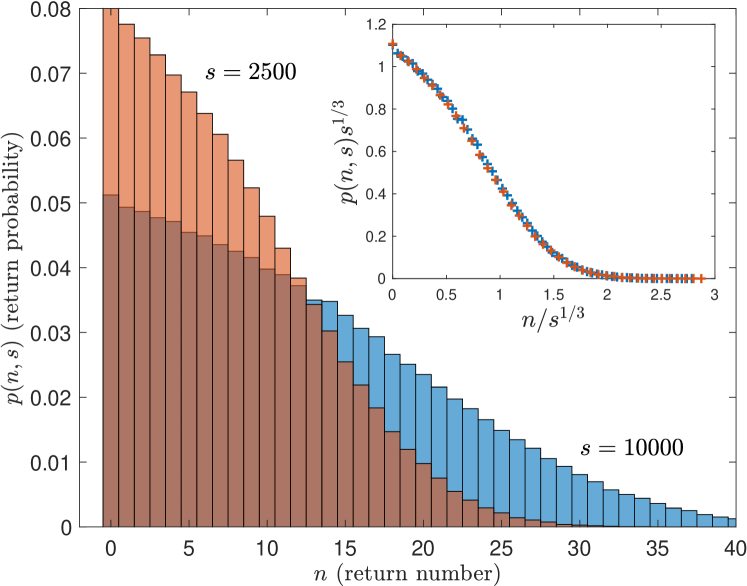
Figure 9: ECMC with factor fields for a 1D Lennard-Jones system ($N=8192$, $T/\epsilon=1$). Probability $p(n,s)$ to return $n$ times to the original active particle during $s$ events (for $s=2500$ and $s=10000$). Mean and standard deviation of $p(n,s)$ both grow as $s^{\gamma/2}\sim s^{1/3}$ (see eq. (27)). Inset: data collapse using scaling variables $p(n,s)s^{1/3}$ vs. $n/s^{1/3}$.

V Conclusions

We have compared in detail the dynamics of three simulation methods (reversible MCMC, MD and ECMC) for 1D systems with local interactions. We have shown that in many situations ECMC displays the same dynamic scaling ($z=1$) as molecular dynamics. Both are asymptotically faster than the diffusive behavior found in MCMC ($z=2$). With a good choice of factors, ECMC is much faster than MD, since it does not need to use a small integration time step to stably explore configurations. Furthermore, unlike MD, ECMC is exact to machine precision, as it is free from time-discretization errors.

Generalizing from the 1D harmonic model, we map 1D systems onto thermodynamically equivalent systems at zero pressure with periodic boundary conditions. This leads to further acceleration of ECMC for both smooth and discontinuous potentials. We have found in this case a remarkably low dynamic exponent ($z=1/2$), better than MD. This acceleration is associated with a modification of the dynamics of the event steps (as a consequence of eq. (1)). Rather than displaying directed motion, the signal $i(s)$ becomes super-diffusive and optimally explores local density fluctuations, being driven forward in regions of high density, and back in regions of low density. A scaling hypothesis predicts a super-diffusive law of the form $\langle i^{2}(s)\rangle\ \sim s^{4/3}$ for the dynamics of the active label as well as an explanation for the emergence of the exponent $z=1/2$.

There is a clear interest in generalizing these results to higher-dimensional models. Already a two and three-dimensional harmonic model has been shown Lei2018b to display accelerated convergence in the ECMC algorithm. In geometries which remain fixed, such as the $XY$ model or fixed harmonic networks (without disorder) it appears possible to implement generalized factor fields. With fluctuating neighbor relations, for instance in a fluid, the generalization of factor fields will represent an interesting challenge Wallace70 .

- (1) N. Metropolis, A. W. Rosenbluth, M. N. Rosenbluth, A. H. Teller, and E. Teller, “Equation of State Calculations by Fast Computing Machines,” J. Chem. Phys., vol. 21, pp. 1087–1092, 1953.
- (2) D. A. Levin, Y. Peres, and E. L. Wilmer, Markov Chains and Mixing Times. American Mathematical Society, 2008.
- (3) W. Krauth, Statistical Mechanics: Algorithms and Computations. Oxford University Press, 2006.
- (4) B. J. Alder and T. E. Wainwright, “Phase Transition for a Hard Sphere System,” J. Chem. Phys., vol. 27, pp. 1208–1209, 1957.
- (5) K. S. Turitsyn, M. Chertkov, and M. Vucelja, “Irreversible Monte Carlo algorithms for efficient sampling,” Physica D: Nonlinear Phenomena, vol. 240, no. 4–5, pp. 410 – 414, 2011.
- (6) Y. Sakai and K. Hukushima, “Dynamics of One-Dimensional Ising Model without Detailed Balance Condition,” Journal of the Physical Society of Japan, vol. 82, no. 6, p. 064003, 2013.
- (7) Y. Sakai and K. Hukushima, “Eigenvalue analysis of an irreversible random walk with skew detailed balance conditions,” Phys. Rev. E, vol. 93, p. 043318, 2016.
- (8) J. Bierkens and A. Bouchard-Côté and A. Doucet and A. B. Duncan and P. Fearnhead and T. Lienart and G. Roberts and S. J. Vollmer, “Piecewise deterministic Markov processes for scalable Monte Carlo on restricted domains,” Statistics & Probability Letters, vol. 136, pp. 148–154, 2018.
- (9) E. P. Bernard, W. Krauth, and D. B. Wilson, “Event-chain Monte Carlo algorithms for hard-sphere systems,” Phys. Rev. E, vol. 80, p. 056704, 2009.
- (10) M. Michel, S. C. Kapfer, and W. Krauth, “Generalized event-chain monte carlo: Constructing rejection-free global-balance algorithms from infinitesimal steps,” J. Chem. Phys., vol. 140, no. 5, p. 054116, 2014.
- (11) E. P. Bernard and W. Krauth, “Two-Step Melting in Two Dimensions: First-Order Liquid-Hexatic Transition,” Phys. Rev. Lett., vol. 107, p. 155704, 2011.
- (12) M. Engel, J. A. Anderson, S. C. Glotzer, M. Isobe, E. P. Bernard, and W. Krauth, “Hard-disk equation of state: First-order liquid-hexatic transition in two dimensions with three simulation methods,” Phys. Rev. E, vol. 87, p. 042134, 2013.
- (13) S. C. Kapfer and W. Krauth, “Two-Dimensional Melting: From Liquid-Hexatic Coexistence to Continuous Transitions,” Phys. Rev. Lett., vol. 114, p. 035702, 2015.
- (14) M. Michel, J. Mayer, and W. Krauth, “Event-chain Monte Carlo for classical continuous spin models,” EPL, vol. 112, no. 2, p. 20003, 2015.
- (15) Y. Nishikawa, M. Michel, W. Krauth, and K. Hukushima, “Event-chain algorithm for the heisenberg model: Evidence for dynamic scaling,” Phys. Rev. E, vol. 92, p. 063306, Dec 2015.
- (16) M. Hasenbusch and S. Schaefer, “Testing the event-chain algorithm in asymptotically free models,” Phys. Rev. D, vol. 98, p. 054502, 2018.
- (17) S. C. Kapfer and W. Krauth, “Irreversible Local Markov Chains with Rapid Convergence towards Equilibrium,” Phys. Rev. Lett., vol. 119, p. 240603, 2017.
- (18) Z. Lei and W. Krauth, “Mixing and perfect sampling in one-dimensional particle systems,” EPL, vol. 124, no. 2, p. 20003, 2018.
- (19) D. Randall and P. Winkler, “Mixing Points on an Interval,” in Proceedings of the Seventh Workshop on Algorithm Engineering and Experiments and the Second Workshop on Analytic Algorithmics and Combinatorics, ALENEX /ANALCO 2005, Vancouver, BC, Canada, 22 January 2005, pp. 218–221, 2005.
- (20) D. Randall and P. Winkler, “Mixing Points on a Circle,” in Approximation, Randomization and Combinatorial Optimization. Algorithms and Techniques: 8th International Workshop on Approximation Algorithms for Combinatorial Optimization Problems, APPROX 2005 and 9th International Workshop on Randomization and Computation, RANDOM 2005, Berkeley, CA, USA, August 22-24, 2005. Proceedings (C. Chekuri, K. Jansen, J. D. P. Rolim, and L. Trevisan, eds.), pp. 426–435, Berlin, Heidelberg: Springer Berlin Heidelberg, 2005.
- (21) Z. Lei and W. Krauth, “Irreversible Markov chains in spin models: Topological excitations,” EPL, vol. 121, p. 10008, 2018.
- (22) M. F. Faulkner, L. Qin, A. C. Maggs, and W. Krauth, “All-atom computations with irreversible Markov chains,” J. Chem. Phys., vol. 149, no. 6, p. 064113, 2018.
- (23) A. C. Maggs, “Multiscale Monte Carlo Algorithm for Simple Fluids,” Phys. Rev. Lett., vol. 97, p. 197802, 2006.
- (24) E. A. J. F. Peters and G. de With, “Rejection-free Monte Carlo sampling for general potentials,” Phys. Rev. E, vol. 85, p. 026703, 2012.
- (25) J. Harland, M. Michel, T. A. Kampmann, and J. Kierfeld, “Event-chain Monte Carlo algorithms for three- and many-particle interactions,” EPL, vol. 117, no. 3, p. 30001, 2017.
- (26) B. J. Alder and T. E. Wainwright, “Decay of the Velocity Autocorrelation Function,” Phys. Rev. A, vol. 1, pp. 18–21, 1970.
- (27) J. P. Wittmer, P. Polińska, H. Meyer, J. Farago, A. Johner, J. Baschnagel, and A. Cavallo, “Scale-free center-of-mass displacement correlations in polymer melts without topological constraints and momentum conservation: A bond-fluctuation model study,” J. Chem. Phys., vol. 134, no. 23, pp. 234901–234901, 2011.
- (28) E. Hairer, C. Lubich, and G. Wanner, Geometric Numerical Integration: Structure-Preserving Algorithms for Ordinary Differential Equations; 2nd ed. Dordrecht: Springer, 2006.
- (29) H. Flyvbjerg and H. G. Petersen, “Error estimates on averages of correlated data,” J. Chem. Phys., vol. 91, no. 1, pp. 461–466, 1989.
- (30) Y. Hu and P. Charbonneau, “Clustering and assembly dynamics of a one-dimensional microphase former,” Soft Matter, vol. 14, no. 20, pp. 4101–4109, 2018.
- (31) T. R. Scavo and J. B. Thoo, “On the Geometry of Halley’s Method,” The American Mathematical Monthly, vol. 102, no. 5, pp. 417–426, 1995.
- (32) S. C. Kapfer and W. Krauth, “Cell-veto Monte Carlo algorithm for long-range systems,” Phys. Rev. E, vol. 94, p. 031302, 2016.
- (33) L. Tonks, “The Complete Equation of State of One, Two and Three-Dimensional Gases of Hard Elastic Spheres,” Phys. Rev., vol. 50, p. 955, 1936.
- (34) K. Kimura and S. Higuchi, “Anomalous diffusion analysis of the lifting events in the event-chain Monte Carlo for the classical XY models,” EPL, vol. 120, no. 3, p. 30003, 2017.
- (35) W. Feller, An introduction to probability theory and its applications. Vol. I. Third edition, New York: John Wiley & Sons Inc., 1968.
- (36) C. Banderier and M. Wallner, “Local time for lattice paths and the associated limit laws,” in Proceedings of the 11th International Conference on Random and Exhaustive Generation of Combinatorial Structures (GASCom 2018), Athens, Greece, June 18-20, 2018. CEUR Workshop Proceedings (L. Ferrari and M. Vamvakari, eds.), vol. 2113, pp. 69–78, CEUR Workshop Proceedings, 2018.
- (37) D. C. Wallace, Thermoelastic Theory of Stressed Crystals and Higher-Order Elastic Constants, vol. 25, pp. 301–404. New York and London: Academic Press, 1970.