Do deviations of neutron scattering widths distribution from the Porter-Thomas law indicate on failure of the Random Matrix theory?

Abstract

Deviations of neutron scattering width distributions from the Porter-Thomas law due to resonances overlapping are calculated in the extended framework of the random matrix approach.

I Introduction

Large irregularities found in spectra in elastic neutron resonant scattering on nuclei are widely accepted as a signature of strong quantum chaos in the internal dynamics of heavy nuclei. The random matrix theory (RMT) Mehta (2004) that presents an approach of extreme chaos is believed to be consistent with the most of nuclear data, nicely reproducing both the nearest neighbor levels spacing distributions and the distributions of the resonances widths.

However, recently it was stated Koehler et al. (2012) that a more careful analysis of old existing datasets Koehler (2011), as well as the new more precise data Koehler et al. (2010) on the neutron resonant scattering indicate on noticeable deviations of widths distribution from the Porter-Thomas (PT) lawPorter and Thomas (1956) . Since the latter was often accepted as a basic prediction of RMT, these deviations were considered in Koehler et al. (2012) as a ground to doubt the validity of RMT approach as itself.

These deviations can be treated as an influence of different other non-chaotic mechanisms (e.g. as the influence of peak of neutron strength function Weidenmüller (2010), parent-daughter correlationsVolya (2011), nonstatistical $\gamma$-decays Volya et al. (2015)) that can cause deviations from “true chaos” expectations. Meanwhile, one should also remind Celardo et al. (2011), that even within the frameworks of RMT the pure Porter-Thomas lawPorter and Thomas (1956) is valid for nonoverlapping resonances only. Actually, already the level and widths joint statistics found in the extended RMT approach Sokolov and Zelevinsky (1989) indicated on the mutual influence between widths and level spacings of resonances, dependent on the overlapping parameter defined as

$$\kappa=\left\langle\Gamma\right\rangle/D,$$ (1)

where $\left\langle\Gamma\right\rangle$ is the mean resonance width and $D$ is the mean level spacing.

Despite to the joint statistics for a set of overlapping neutron resonances with their energy levels and widths distributions in the frameworks of RMT is known for a long time ago Sokolov and Zelevinsky (1989) (see also Fyodorov et al. (1997), and references therein), the joint widths and levels distribution obtained in Sokolov and Zelevinsky (1989) can hardly be directly applied to available experimental data (like in Koehler et al. (2012)) in order to test whether the deviations from PT law are compatible with expectations within RMT. Instead of joint distribitions dependent on all the widths and level positions one needs for more practical, so called “inclusive” width distribution, e.g. the distribution of width for some given resonance, that is averaged over widths and positions of all the rest ones. However, this distribution was not yet obtained in the clear explicit form, that cause some challenge Shchedrin and Zelevinsky (2012); Fyodorov and Savin (2015); Bogomolny (2016) to get corresponding analytical estimates.

Another problem that deserves to be mentioned is also the notorious “semi-circle” law, the inherent prediction of RMT for global distribution of levels, that has no common with actual level distributions in nuclei. This implies that only a small part of levels far enough from boundaries and located in center of the “semi-circle” is relevant for comparison with data. A way to cure this problem imposing in the level space periodic boundary conditions was proposed by Dyson Dyson (1962a, b, c) with the approach based on circular ensembles of random matrices. Within this approach all the levels are “central” with same level density in contrast to traditional RMT.

One may expect that local predictions of both approaches, for central levels in RMT and levels in circular ensembles, taken at the same mean level density, should be the same in the limit $N\to\infty$, where $N$ is the total number of levels. This equivalence of RMT and circular ensembles in application to particular systems (e.g. nuclei) is actually based on the implicit assumption, that the relevant quantities are formed locally, inside the range of levels energy, where the level density can be considered to be approximately constant.

This idea were actually employed in the work Shchedrin and Zelevinsky (2012) where an unphysical global “semi-circle” law was simply replaced by constant levels density spanned over infinite range of energy. In turn, the form of local mutual influence of resonances (including its particular pairwise structure) was inherited from RMT Sokolov and Zelevinsky (1989).

An important gain of the work Shchedrin and Zelevinsky (2012) is that local resonance-to-resonance interaction form coming from extreme chaos assumptions is sepatated from the model-specific global distribution of levels over energy: accepting the former one may replace the latter by some more realistic one.

Intuitively this idea is supported by an analogy between the level-width system and log gas of charged particles (see, e.g. Dyson (1962a, b, c); Sommers et al. (1988); Haake et al. (1992); Forrester (2016)). Moreover one can expect for some parameter like Debye screening length that separates the particular interactions of nearest neighbors from the mean field influence of far particles.

Unfortunately, the estimates of width distribution presented in Shchedrin and Zelevinsky (2012) were restricted by one more simplifying ansatz, that takes the levels be “pinned” at fixed positions equidistantly in energy. This ansatz simplify calculations substantially, but it appears to be too crude for nearest neighbors contribution. In fact, the pairwise resonances interaction is strongly enhanced at their small separations, and an account for variations of spacings between the resonance and its nearest neighbors requires a more accurate estimate.

In this work we calculate the width distribution with an explicit integration over small spacings between the resonance and its two nearest neighbors, while the contribution of the rest far resonances will be estimated within the equidistant approach used in Shchedrin and Zelevinsky (2012). The result is presented in a simple analytical form suitable for comparison with experiments. In order to verify the estimate we develop a numerical approach that allows to simulate the statistics of levels and width, suitable for study of RMT predictions in a clear transparent way. We demonstrate that our analytical estimate is in a reasonable agreement with numerical simulations.

In Sect.II we explore the extended RMT expression Sokolov and Zelevinsky (1989) for joined neutron resonances widths and levels statistics, and segregate local pairwise resonance interactions apart a global potential that cause the level density distribution to be “semi-circle”. This allows to introduce a simple model that is free from the notorious semi-circle law, that can be very useful in numerical simulations and analytical estimates. To get a more physical insight in Sect.B we perform the simulations and found that for the overlapping parameter $\kappa\lesssim 0.3$ (far from the width collectivization border Sokolov and Zelevinsky (1992) at $\kappa\sim 1$). Then, with experience of the numerical simulations we get an analytical estimates that agree well with the numerical data.

II Different scales in RMT: domain of chaos and the semicircle law

In the work Sokolov and Zelevinsky (1989) the standard random matrices theory Mehta (2004) was extended to unstable states. In the case of one open channel the joint distribution for energies $\vec{E}=\{E_{n}\}$ and widths $\vec{\Gamma}=\{\Gamma_{n}\}$ ($n=1,\ldots,N$) were found in the form:

$$\mathrm{d}{\cal P}(\vec{E};\vec{\Gamma})=C_{N}\cdot\left(\frac{1}{a}\right)^{\frac{N(N+1)}{2}}\left(\frac{N}{2\pi\eta}\right)^{\frac{N}{2}}\times$$

$$\quad\times\prod_{m<n}\frac{(E_{m}-E_{n})^{2}+\frac{1}{4}(\Gamma_{m}-\Gamma_{n})^{2}}{\sqrt{(E_{m}-E_{n})^{2}+\frac{1}{4}(\Gamma_{m}+\Gamma_{n})^{2}}}$$

$$\quad\times\exp\left[-N\left(\frac{1}{a^{2}}\sum_{n}E_{n}^{2}+\frac{1}{2a^{2}}\sum_{m<n}\Gamma_{m}\Gamma_{n}+\frac{1}{2\eta}\sum_{n}\Gamma_{n}\right)\right]$$

$$\quad\times\prod_{n}\mathrm{d}E_{n}\frac{\mathrm{d}\Gamma_{n}}{\sqrt{\Gamma_{n}}}.$$ (2)

where, according to Sokolov and Zelevinsky (1989); Mehta (1960), the normalization constant

$$C_{N}=N^{\frac{N(N+1)}{4}}2^{\frac{N(N-1)}{4}}\frac{1}{N!}\left[\prod_{n=1}^{N}\Gamma(n/2)\right]^{-1}.$$ (3)

Here the parameter $a$ controls the energy range occupied by levels, while $\eta$ is related with the mean level width $\langle\Gamma\rangle$ by condition $\eta=N\langle\Gamma\rangle$.

In the limit $N\to\infty$ all the levels are distributed inside the energy interval $(-a,a)$ by a famous “semi-circle” law:

$$\frac{\mathrm{d}n}{\mathrm{d}E}=N\frac{2}{\pi a}\sqrt{1-(E/a)^{2}}.$$ (4)

The chaotic nature of RMT manifests itself in the level spacing statistics and local correlations of levels, while the global envelope (4) is nothing but kinematical restrictions of Wigner RMT model, that consider $N$ initially degenerated levels with $E=0$ spread over “semi-circle” by finite random interactions. Obviously, the width distribution of resonances depends on whether the resonance is placed at the center of the “semi-circle” or near its boundary at $E=\pm a$.

In order to decrease the influence of bounds at $E=\pm a$, one may consider the resonances lying inside a domain

$$-\Delta<E<\Delta$$ (5)

with $\Delta\ll a$, where the local mean level spacing $D=\pi a/2N$ is approximately constant:

$$D^{-1}=\frac{\mathrm{d}n}{\mathrm{d}E}=N\frac{2}{\pi a}\left(1-O(\Delta^{2}/a^{2})\right)\approx\mathrm{const}.$$ (6)

In addition, one should also require that size of this domain $\Delta$ is still large compared to any correlation length.

Due to symmetry of the distribution (2) around $E=0$, it is convenient to define the index range as $m,n\in(-L,\ldots,0,\ldots,L)$, where $N=2L+1$. Moreover, due to symmetry of the Eq.(2) with respect to any permutation inside the set of pairs $\left\{(E_{n},\Gamma_{n})\right\}$, without any loss of generality, one can consider the set of pairs $(E_{n},\Gamma_{n})$ be ordered in energy: $E_{m}<E_{n}$ for any $m<n$, so the pair with $n=0$ appears near the maximum of the distribution (4) .

Now, let us note that all the local properties including levels and widths distribution inside the domain 5 is governed only by the two parameters, by the mean level spacing $D$ and the mean width $\langle\Gamma\rangle$. Using $D$ as a natural energy scale, one may introduce dimensionless variables

$$\varepsilon_{n}=E_{n}/D,\qquad x_{n}=\Gamma_{n}/\kappa D=\Gamma_{n}/\langle\Gamma_{n}\rangle.$$ (7)

that emphasize the scaling properties of levels system inside the central domain (5).

With these notations the joint distribution (2) can be rewritten as

$$\mathrm{d}\bar{\mathcal{P}}(\vec{\varepsilon};\vec{x})=\bar{C}(N)\times$$

$$\qquad\times\left\{\prod_{n}\exp\left(-\frac{\pi^{2}}{4N}\varepsilon_{n}^{2}\right)\times\exp\left(-\frac{1}{2}x_{n}\right)\right\}$$ (8)

$$\qquad\times\prod_{m<n}\frac{(\varepsilon_{m}-\varepsilon_{n})^{2}+\frac{\kappa^{2}}{4}(x_{m}-x_{n})^{2}}{\sqrt{(\varepsilon_{m}-\varepsilon_{n})^{2}+\frac{\kappa^{2}}{4}(x_{m}+x_{n})^{2}}}$$ (9)

$$\qquad\qquad\times\exp\left(-\frac{\pi^{2}\kappa^{2}}{8N}x_{m}x_{n}\right)\prod_{n}\mathrm{d}\varepsilon_{n}\frac{\mathrm{d}x_{n}}{\sqrt{2\pi x_{n}}}.$$ (10)

Here the normalization constant

$$\bar{C}(N)=(\pi/2)^{N(N+1)/2}2^{N(N-1)/4}\prod_{n=1}^{N}\left[\Gamma(n)\right]^{-1}$$ (11)

is defined here by the integration over the ordered domain

$$\varepsilon_{-L}<\varepsilon_{-L+1}<\ldots<\varepsilon_{0}<\ldots<\varepsilon_{L-1}<\varepsilon_{L}.$$

III The analog statistical mechanics problem.

It is very instructive to examine the joint distribution of $N$ levels and their widths in terms of an analog statistical mechanics problem, as the Boltzmann distribution of $N$ interacting particles that are posed into a thermal bath Dyson (1962a); Haake et al. (1992) (see also the textbook Mehta (2004)). In this way the joint probability distribution (8)-(10) can be considered as some partition function

$$\mathrm{d}\bar{\mathcal{P}}(\vec{\varepsilon};\vec{x})=\mathcal{Z}^{-1}\exp(-U(\vec{\varepsilon};\vec{x})/T)\prod_{n}\mathrm{d}\varepsilon_{n}\frac{\mathrm{d}x_{n}}{\sqrt{2\pi x_{n}}}$$ (12)

In statistical mechanics this is a typical starting point to deduce the properties of the system, e.g. single particle distributions, particles correlations, critical phenomena, etc. It is also very convenient for computer simulations (see, e.g. many examples in Binder (1986)), that allows to obtain the distribution directly “from the first principles”, without any further approximations in the partition function, that are unavoidable in analytical study. In turn, the analytical study, enhanced by the analogy with a condensed matter problem, can provide us better understanding the physical properties of the system. Below we use both of them, in order to justify numerically the assumptions that underlies the analytical approach used below, as well as to test the final results with numerical experiments.

Let us consider the analog statistical problem in more details. Without any loss of generality hereafter one can put ${T=1}$. For further convenience one can change the variables $x_{n}\to\xi_{n}^{2}$, that turns the Porter-Thomas distribution into a more usable nonsingular form:

$$\exp(-x/2)\frac{\mathrm{d}x}{\sqrt{2\pi x}}\to\exp(-\xi^{2}/2)\frac{\mathrm{d}\xi}{\sqrt{2\pi}},$$ (13)

where the range of $\xi_{n}$ is defined as $\xi_{n}\in(-\infty,\infty)$.

Now we have a statistical system of $N$ particles in two-dimensional space $(\varepsilon,\xi)$. According to (12) and (8)-(10) the potential energy $U(\vec{\varepsilon},\vec{\xi})$ can be splitted into three terms

$$U(\vec{\varepsilon},\vec{\xi})=U^{g}(\vec{\varepsilon})+U^{PT}(\vec{\xi})+U^{int}(\vec{\varepsilon},\vec{\xi}).$$ (14)

where the potentials

$$U^{g}(\vec{\varepsilon})=\sum_{n=-L}^{L}\frac{\pi^{2}}{4N}\varepsilon_{n}^{2}$$ (15)

and

$$U^{PT}(\vec{\xi})=\sum_{n=-L}^{L}\frac{1}{2}\xi_{n}^{2}$$ (16)

confine the system along $\varepsilon$ and $\xi$ directions, respectively.

The mutual particle to particle interactions are repulsive and have a pairwize form:

$$U^{int}(\vec{\varepsilon},\vec{\xi})=\frac{1}{2}\sum_{m\neq n}U^{int}(\varepsilon_{m}-\varepsilon_{n},\xi_{m},\xi_{n})=$$

$$\quad=-\frac{1}{2}\sum\limits_{m\neq n}\log\frac{(\varepsilon_{m}-\varepsilon_{n})^{2}+\frac{\kappa^{2}}{4}(\xi_{m}^{2}-\xi_{n}^{2})^{2}}{\sqrt{(\varepsilon_{m}-\varepsilon_{n})^{2}+\frac{\kappa^{2}}{4}(\xi_{m}^{2}+\xi_{n}^{2})^{2}}}$$ (17)

$$\qquad+\frac{1}{2}\sum\limits_{m\neq n}\frac{\pi^{2}\kappa^{2}}{8N}\xi_{m}^{2}\xi_{n}^{2}.$$ (18)

The sum $(U^{g}(\varepsilon)+U^{PT}(\xi))$ presents a global potential well. In the limit $N\gg 1$ this well is stretched along the $\varepsilon$-direction, so the system forms a chain of particles lined along the $\varepsilon$-axis.

In the limit $\kappa\to 0$ the particle-particle interaction terms (17)-(18) turns into a much simpler form

$$U^{int}_{mn}=-\log|\varepsilon_{m}-\varepsilon_{n}|.$$ (19)

that describesDyson (1962b) electrostatic repulsion between particles of unit charge in two-dimensional electrodynamics. As a balance between the global contracting potential $U^{g}(\varepsilon)$ and repulsive interparticle interaction terms $U^{int}_{mn}$, in presence of the thermal bath with $T=1$ the density of particle distribution takes in the limit $N\gg 1$ the “semi-circle” form

$$\frac{\mathrm{d}n}{\mathrm{d}\varepsilon}=\sqrt{1-(2\varepsilon/N\pi)^{2}}.$$ (20)

where the semicircle radius $\bar{a}\to\pi N/2$ grows with $N$ linearly. In turn, the spacing distribution of neighbor particles is known to be close to the Wigner surmise

$$\frac{\mathrm{d}w}{\mathrm{d}s}=\frac{1}{2\bar{s}}\exp\left(-\pi s^{2}/4\bar{s}^{2}\right).$$ (21)

where the mean spacing $\bar{s}=(\frac{\mathrm{d}n}{\mathrm{d}\varepsilon})^{-1}$.

The analog statistical system is in fact the Wigner crystalWigner (1934) of charged particles that is posed into the global potential $U^{g}(\varepsilon)=(\pi^{2}/4N)\varepsilon^{2}$. The role of the potential $U^{g}(\varepsilon)$ is two-fold:

• it provides the boundary conditions that hold the particles together preventing the system from expansion due to electrostatic repulsion of particles, and

• it deforms the crystal, modulating the particle density by a (rather unphysical) semi-circle law form (20).

Apart from the long-range global particle density modulation there are local particle correlations due to their mutual interactions (17),(18). This correlation effects involve mainly nearest partners, while the influence of distant partners acts effectively as some mean field, and is generally responsible for the global modification of particle distribution. If the corresponding correlation length (the “Debye screening” parameter) $\lambda_{\varepsilon}\ll\bar{a}$, all the correlation effects are expected to be local phenomena, that are governed by the local particle density and practically independent of the crystal boundary conditions. Then the condition (5) turns into

$$-\Delta_{\varepsilon}<\varepsilon<\Delta_{\varepsilon},$$ (22)

where $\Delta_{\varepsilon}$ obeys the restrictions $\Delta_{\varepsilon}\gg\lambda_{\varepsilon}$ and $\Delta_{\varepsilon}\ll\bar{a}$. The latter restriction provides, that in this domain the mean particle spacing $\bar{s}$ is approximately constant

$$(\bar{s})^{-1}=1-\frac{1}{2}(2\varepsilon/N\pi)^{2}+\ldots\approx 1,$$

and the mean positions of particles inside the domain (22) can be considered as equidistant Shchedrin and Zelevinsky (2012).

III.1 A map on a circle: a way to get rid of semicircle law.

A radical way to get rid of the semicircle law for level energy distribution is to map the energies of particles onto the unit circle as it was proposed by Dyson Dyson (1962a, b):

$$\varepsilon\in(-L,\ldots,0,\ldots,L)\to\theta\in(-\pi,\ldots,0,\ldots,\pi).$$ (23)

In fact, Dyson had considered inDyson (1962a, b, c) circular ensembles of random unitary matrices for closed systems of stable levels with zero widths. Extention of circular ensembles to open systems was given in later works Fyodorov and Sommers (2000); Fyodorov (2001) and in the recent work Killip and Kozhan (2016) the join distribution for levels and width was obtained for any $\beta$, that includes $\beta=1$ ($T$-invariant), $\beta=2$ ($T$-noninvariant) and $\beta=2$ (symplectic) ensembles.

Here we restrict ourselves by the $T$-invariant case, and consider the RMT joint distribution (2) with minimalistic modifications. Using the map (23) we we make the substitution

$$(\varepsilon_{m}-\varepsilon_{n})^{2}\to\left|\mathrm{e}^{i\frac{2\pi}{N}\varepsilon_{m}}-\mathrm{e}^{i\frac{2\pi}{N}\varepsilon_{n}}\right|^{2}\left(\frac{N}{2\pi}\right)^{2}$$ (24)

into eq.(17). We refer this model as circularly modified RMT (cmRMT) .

Geometrically, in this model the particles (levels) are placed on the surface of the unit radius cylinder. Their positions in $\{\varepsilon_{n}\}$ are mapped onto the cylinder directrix, while the positions in $\xi_{n}$ are mapped along cylinder generatrices. Along $\xi$ particles are kept by the potential (16) and particle-particle interaction terms

$$U^{int}(\vec{\varepsilon},\vec{\xi})=-\frac{1}{2}\sum\limits_{m\neq n}\log\frac{\left|\mathrm{e}^{i\frac{2\pi\varepsilon_{m}}{N}}-\mathrm{e}^{i\frac{2\pi\varepsilon_{n}}{N}}\right|^{2}\left(\frac{N}{2\pi}\right)^{2}+\frac{\kappa^{2}}{4}(\xi_{m}^{2}-\xi_{n}^{2})^{2}}{\sqrt{\left|\mathrm{e}^{i\frac{2\pi\varepsilon_{m}}{N}}-\mathrm{e}^{i\frac{2\pi\varepsilon_{n}}{N}}\right|^{2}\left(\frac{N}{2\pi}\right)^{2}+\frac{\kappa^{2}}{4}(\xi_{m}^{2}+\xi_{n}^{2})^{2}}}+\frac{1}{2}\sum\limits_{m\neq n}\frac{\pi^{2}\kappa^{2}}{8N}\xi_{m}^{2}\xi_{n}^{2}.$$ (25)

Let us stress, that in cmRMT model all the levels are placed homogeneously on the compact unit circle. The “global” potential (15) that had kept levels inside the range $\varepsilon\in\{-\frac{\pi N}{2},-\frac{\pi N}{2}\}$ in the original RMT Sokolov and Zelevinsky (1989) is here irrelevant and should be omitted. Obviously, in the limit $N\to\infty$ predictions of of cmRMT and RMT models coincide.

Due to periodicity along the axis $\varepsilon$ all the levels have the same mean spacing and the same width distribution. This is very advantages in numerical simulations of the system, since the statistics can be substantially improved by averaging the width distribution over all the levels, rather than over a small subset of levels (22) around the center of the semicircle (20) in the original RMT.

However, one should admit that the original RMT appears to be more convenient to get analytical approach for the level width distribution.

III.2 Non-overlapping resonances ($\kappa=0$).

In the limit of non-overlapping resonances ($\kappa=0$) width and level distributions decouples, with the same Porter-Thomas width distribution for all the levels. The level energies distribitions are

$$\propto\prod_{m,n}|\varepsilon_{n}-\varepsilon_{m}|\times\exp\left\{-\sum_{n}\frac{\pi^{2}}{4N}\varepsilon_{n}^{2}\right\}$$ (26)

for RMT model, while cmRMT model the distribution

$$\propto\prod_{m,n}\left|\mathrm{e}^{i\frac{2\pi}{N}\varepsilon_{m}}-\mathrm{e}^{i\frac{2\pi}{N}\varepsilon_{n}}\right|$$ (27)

coinsides with corresponding distribution in Dyson (1962a) for Dyson’s $T$-invariant circular random ensemble.

III.3 Overlapping resonances ($\kappa\neq 0$).

The Breight-Wigner widths of neutron scattering resonances are in practice finite, and the resonances can overlap: $\kappa=\langle\Gamma\rangle/D>0$.

In terms of the analog statistical model, at $\kappa\neq 0$ the particle to particle interactions, given by eqs.(17-18) depend not only on the separations along the axis $\varepsilon$ but on the positions in $\xi$ as well. This extra dependence on $\xi$ causes the deviations in particle distribution along $\xi$ from the normal law that is provided by the potential $U^{PT}(\xi)=\xi^{2}/2$ (16): the normal law becomes valid only in the limit $\kappa\to 0$. In terms of the original neutron resonant scattering problem this fact results in deviations of the neutron scattering width distributions from the famous Porter-Thomas law.

Let us analyse the interaction terms (17-18) in more details.

The term (18) describes the interactions that causes anticorrelations between $\xi_{m}^{2}$ and $\xi_{n}^{2}$ for any pair $(m,n)$. It is curious that these anticorrelations are completely independent of the pair spacing $|\varepsilon_{m}-\varepsilon_{n}|$. Despite to that each pair contribution drops with $N$ as $N^{-1}$, for any given $n$-th particle the net effect coming from all $(N-1)$ its partners in the limit $N\to\infty$ remains finite so the sum over all the partners acts effectively as some mean field: $N^{-1}\sum_{m\neq n}\xi^{2}_{m}=\langle\xi^{2}\rangle+O(N^{-1/2})$. In this way the term (18) turns into :

$$\frac{1}{2}\sum\limits_{m\neq n}^{N}\frac{\pi^{2}\kappa^{2}}{8N}\xi_{m}^{2}\xi_{n}^{2}\to\frac{\pi^{2}\kappa^{2}}{8}\langle\xi^{2}\rangle\sum_{n}\xi_{n}^{2}.$$ (28)

Below we restrict ourselves by the case $\kappa\ll 1$, far from the regime of superradiance transitionSokolov and Zelevinsky (1989) that takes place at $\kappa\sim 1$. At small $\kappa$ one has $\langle\xi^{2}\rangle=1+O(\kappa^{2})$, and with an accuracy sufficient for our purposes one can safely put hereafter $\langle\xi^{2}\rangle=1$. Finally, this term results in some modification of the potential $U^{PT}(\xi)(\ref{eq:U-PT})$:

$$U^{PT}(\xi)\to\tilde{U}^{PT}(\xi)=\frac{1}{2}\left(1+\frac{\pi^{2}\kappa^{2}}{4}\right)\xi^{2}$$ (29)

Now, let us consider the mutual particle interactions given by eq.(17). In contrast to (18), the contribution of any pair $(m,n)$ in the sum (17) is dependent not only on the particles positions $\xi_{m},\xi_{n}$, but on their $\varepsilon$-spacing $s_{mn}=|\varepsilon_{m}-\varepsilon_{n}|$ as well. Expansion in series over $\kappa\ll 1$ gives:

$$\log\left[\frac{s_{mn}^{2}+\frac{\kappa^{2}}{4}(\xi_{m}^{2}-\xi_{n}^{2})^{2}}{\sqrt{s_{mn}^{2}+\frac{\kappa^{2}}{4}(\xi_{m}^{2}+\xi_{n}^{2})^{2}}}\right]=$$

$$\qquad\qquad=\log(s_{mn})-\frac{3\kappa^{2}\xi_{m}^{2}\xi_{n}^{2}}{4s_{mn}^{2}}+\frac{\kappa^{2}(\xi_{m}^{4}+\xi_{n}^{4})}{8s_{mn}^{2}}+\dots.\quad$$ (30)

It is seen, that the second term in the expansion is responsible for anticorrelations between $\xi_{m}^{2}$ and $\xi_{n}^{2}$ while the third term causes deviation from the original distribution due to extra dependence on $\xi_{n}^{4}$.

Both of these contributions are proportional to $s_{mn}^{-2}$ and are enhanced at small spacings $s_{mn}\ll 1$, and their weights become order of unity at spacing

$$s_{mn}\lesssim\max(\kappa\xi_{m}^{2},\kappa\xi_{n}^{2}).$$ (31)

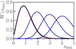
Figure 1: Probability distribution of inter-particle spacing $s_{mn}=|\varepsilon_{k}-\varepsilon_{l}|$ for nearest neighbors $m=n\pm 1$ (black line) and for next to nearest neighbors $m=n\pm(j+1)$, with $j=1,2,3$ (blue lines). The dashed magenta line show the modified Wigner surmise (see text for explanations). Parameters used in numerical simulations are $N=321$, $\kappa=0.1$, the data are averaged over central levels with $m,n\in(-30,30)$.

In turn, the distribution of spacings $s_{mn}$ is crucially dependent on whether the particles $(m,n)$ are nearest neighbors or not. In Fig.1 we illustrate this by plotting the data taken from numerical simulations for the partition function (12) with $U(\vec{\varepsilon},\vec{\xi})$ given by (15)-(18) at $\kappa=0.1$ and $N=321$. The spacings were measured for particles lying in the center of the crystal with $m,n\in(-30,30)$, that correspond to $\Delta_{\varepsilon}\approx 30\ll\bar{a}\approx 504$.

One can see that the distribution of spacings $s_{mn}$ for nearest neighbors ($m=n\pm 1)$ (black line) at $s_{mn}\ll 1$ drops only linearly that being combined with expansion (30) gives singularity $s_{mn}^{-1}$ resulting in logarithm enhancement for contribution of small spacing.

In contrast, for pairs sandwiched by one and more particles ($j=1,2,3,\ldots$) the distribution of spacings shown by blue lines are highly suppressed at $s_{mn}\to 0$. Note, that in the latter case the distributions are peaked approximately at $s_{mn}\approx(j+1)$ and corresponding contribution can be estimated with some reasonable accuracy under assumption that the far partners are placed at fixed equidistant positions with $s_{mn}=2,3,\ldots$, like it was proposed inShchedrin and Zelevinsky (2012).

While far partners can be assumed to be placed equidistant, for nearest neighbors one need know actual distribution of spacings $s_{n,n\pm 1}$. Fortunately, it is remarkably close to the Wigner surmise (21) slightly modified as

$$\frac{\mathrm{d}w}{\mathrm{d}s}=\mathrm{const}\sqrt{s^{2}+(\kappa/2)^{2}}\exp(-\pi s^{2}/4).$$ (32)

(see dashed magenta curve at Fig.1). Below we use this fact in our analytical estimates.

IV Width distribution of overlapping resonances

The resonance width distribution $\mathbb{P}(x,\kappa)$ that we are going to estimate analytically is related in the analog statistical model to the distribution $P(\xi)$ of the particle along the axis $\xi$:

$$\mathbb{P}(x,\kappa)\mathrm{d}x = 2P(\xi,\kappa)\mathrm{d}\xi{\Big{|}}_{\xi=\sqrt{x}}$$ (33)

$$= P(\xi=\sqrt{x},\kappa)\frac{\mathrm{d}x}{\sqrt{x}}$$

In order to minimize the influence of kinematic boundaries in RMT, we consider a central particle (with $n=0$) equally far distant from ends of the system:

$$P(\xi_{0},\kappa,L)=Z^{-1}\int\mathrm{d}s_{-}\,\mathrm{d}s_{+}\prod_{n=-L}^{-1}\mathrm{d}\xi_{n}\prod_{n^{\prime}=1}^{L}\mathrm{d}\xi_{n^{\prime}}\times$$

$$\quad\times\exp\left[-\sum_{n=-L}^{L}\tilde{U}^{PT}(\xi_{n})-\sum_{m\neq n}\tilde{U}_{2}^{int}(\varepsilon_{m}-\varepsilon_{n};\xi_{m},\xi_{n})\right],$$

where for the central partice we can put $\varepsilon_{0}=0$, and for the nearest neighbor separations $s_{\pm 1}=\varepsilon_{\pm 1}$, while far partners are taken like in Shchedrin and Zelevinsky (2012) at equidistant positions: $\varepsilon_{n}=n$, for $n=\pm 2,\pm 3,\ldots,\pm L$.

Then the integration over the far partner variables $\xi_{n}$, $n=\pm 2,\pm 3,\ldots,\pm L$ can be perfomed by the saddle point method and we get in the limit $L\to\infty$ (see AppendixA):

$$P(\xi_{0}=\sqrt{x},\kappa)=C(\kappa)\times\mathcal{A}(x,\kappa)\times$$

$$\quad\times\exp\left\{-\left(1+\frac{\pi^{2}\kappa^{2}}{4}\right)\frac{x}{2}\right\}\times\mathcal{I}_{0}(x,\kappa)\mathcal{I}_{1}(x,\kappa)$$ (35)

where the contribution coming from far partners is given by the factor

$$\mathcal{A}(x,\kappa) = \left(\frac{\sinh(\pi\kappa/2)}{\pi\kappa/2}\right)^{2}\frac{\pi\kappa\sqrt{2x(3+x)}/4}{\sinh(\pi\kappa\sqrt{2x(3+x)}/4)}\times$$ (36)

$$\times\frac{\left[1+3x\kappa^{2}/8\left(1+x^{2}\kappa^{2}/4\right)\right]}{\left(1+x^{2}\kappa^{2}/4\right)}$$

while the integrals (with $l=1,2$)

$$\mathcal{I}_{l}=\int\mathrm{d}\varepsilon\;\mathrm{d}\xi\frac{\varepsilon^{2}+\frac{\kappa^{2}}{4}\left(\xi^{2}-x\right)^{2}}{\sqrt{\varepsilon^{2}+\frac{\kappa^{2}}{4}\left(\xi^{2}+x\right)^{2}}}\times$$

$$\mathrm{e}^{-\xi^{2}/2}\varepsilon^{l}\exp\left\{-\frac{(1+\pi/4)^{2}}{\sqrt{\pi}\varepsilon^{2}}\right\}$$ (37)

This integrals can be easily be either evaluated numerically or estimated analyticaly.

The normalization factor $C(\kappa)$ is fixed by a condition

$$\int\limits_{-\infty}^{\infty}P(\xi_{0})\mathrm{d}\xi_{0}=\int\limits_{0}^{\infty}\mathbb{P}(x)\mathrm{d}x=1.$$ (38)

The effect of resonances interactions on the width distribution is better seen in the ratio of $\mathbb{P}(x,\kappa)=P(\xi_{0}=\sqrt{x},\kappa)/\sqrt{x}$ to the Porter-Thomas distribution $W_{PT}(x)=\exp(-x/2)/\sqrt{2\pi x}$:

$$\Psi(x|\kappa)=\mathbb{P}(x,\kappa)/W_{PT}(x)=$$

$$\quad=\pi C(\kappa)\mathcal{A}(x,\kappa)\exp\left\{-\frac{\pi^{2}\kappa^{2}}{8}x\right\}\mathcal{I}_{0}(x,\kappa)\mathcal{I}_{1}(x,\kappa)$$

(39)

Indeed, the normalization factor $C(\kappa)$ can also be fixed by the condition

$$\int_{0}^{\infty}\frac{\mathrm{d}x}{\sqrt{2\pi x}}\;\Psi(x|\kappa)\mathrm{e}^{-x/2}=1.$$ (40)

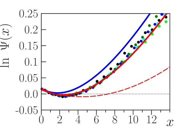
Figure 2: $\log\Psi(x|\kappa)$ for $\kappa=0.05$. Red line presents our analytical estimate given by eq.(39). Results of our numerical simulations of the RMT joined probability distribution (2) (see App.B) are shown by colored points: $N=3$ (lime), $N=5$ (cyan), $N=9$ (green), $N=11$ (blue) and $N=101$ (black ). The red dashed lines show results of the equidistant estimate (see text). The blue line plots recent results obtained by Fyodorov and Savin Fyodorov and Savin (2015).

Let us start with the case of weak overlap $\kappa=0.05$, see Fig..2. the corrected $\Psi(x|\kappa)$ is compared to results of our numerical simulations for direct the RMT joint distribution (2) (see for details Appendix B). In these simulations we perform runs with the number of levels varied from $N=3$ to $N=101$. We see that our analytical estimate (39) agrees well with numerical data. The red dashed lines show the expectations of the “equidistant” ansatz, that assumes that all the resonances are placed on equidistant positions, like it was done in Shchedrin and Zelevinsky (2012). It is clearly seen that the nearest neighbor position fluctuations play a very important role (especially at smaller overlapping parameter $\kappa$). We plot also recent results obtained in the work Fyodorov and Savin (2015). Despite to the qualitative behavior is similar, quantitatively the effects of the resonance overlapping is a bit overestimated.

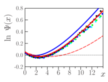
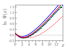
Figure 3: $\Psi(x|\kappa)$ for $\kappa=0.1$ (left) and $\kappa=0.2$ (right). Red solid lines present analytical estimate by eq.(39). Colored points show results of obtained from numerical simulations of the joined probability distribution (2) with $N=321$, $k\in(-30,30)$ (black), $N=161$, $k\in(-10,10)$ (blue), $N=81$, $k\in(-8,8)$ (green), $N=41$, $k\in(-4,4)$ (cyan) and $N=21$, $k\in(-4,4)$ (lime). The red dashed lines show results of the equidistant estimate (see text). Blue lines show the estimates obtained in the recent work Fyodorov and Savin (2015).

The results for $\kappa=0.1$ and $0.4$ are presented in Fig.3. The estimate (39) fit the data well up to $\kappa\lesssim 0.4$. Note also, that at higher $\kappa$ the difference between (39) and analytical estimate given in Fyodorov and Savin (2015) decreases .

In the simulations presented here all the data are collected from the levels lying either at the center or in the central domain with $k\in(-0.1N,0.1N)$. One can see that already at $N\gtrsim 50$ the width distributions of levels lying in the selected domain of $k$ are practically independent of $N$ and reaches its asymptotic behaviour expected in the limit $N\to\infty$, provided that $\kappa\lesssim 0.5$.

However, at $\kappa\gtrsim 0.4$ the width distributions of levels lying even near the center are found to be dependent on total number of levels $N$, and the asymptotic behavior does not occur even at $N\gtrsim 200-300$. To our mind this indicates on long-range correlations that come into play at large overlapping parameter $\kappa$ due to proximity of super-radiance transition that is expected at $\kappa=1$ Sokolov and Zelevinsky (1989).

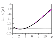
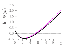
Figure 4: $\Psi(x|\kappa)$ for $\kappa=0.05$ (left) and $\kappa=0.4$ (right). Black and magenta lines present results of simulation for cmRMT ($N=100$) and original RMT ($N=101$). In the latter case the data are taken for levels lying in the central band $k\in(-11,11)$.

To complete this section let us also consider the predictions of circularly modified RMT (cmRMT), introduced in the Section III.1. In Fig.4 we demonstrate that the results are practically identical. However, while with cmRMT we average data over all the levels, in the case of original RMT we must restrict ourselves by a small subset of levels lying at the center of the semicircle.

V Conclusions.

In this paper the deviations of width distributions from the Porter-Thomas law expected in the extended framework of RMT are explicitly calculated in a clear transparent way. Our analytical estimate is in nice agreement with corresponding numerical simulations. The contribution to deviations comes from two sources: the long range correlations calculated in equidistant approximationShchedrin and Zelevinsky (2012) and short-range correlations found in the nearest neighbors approximation. The role of short-range correlations are found especially important at small $\kappa$ where it is logarithmically enhanced.

These deviations from the Porter-Thomas law occur even the dynamics inside the system is perfectly chaotic, irrespective to possible existence of contributions coming from other mechanisms Weidenmüller (2010); Celardo et al. (2011); Volya (2011); Volya et al. (2015) that can also cause the deviations from the Porter-Thomas law. Despite to a comparative analysis of all this sources is very interesting, in this paper we restrict ourselves by effects survive in the limit of the perfect chaos.

VI Acknowledgments

I am are very grateful V.V. Sokolov for many years collaboration and many stimulative discussions that cause my interest to this topic. This work is supported by the Ministry of Education and Science of the Russian Federation.

Appendix A Calculation of the width distribution (IV)

The distribution of the central particle with $n=0$ along the axis $\xi$ is given by the expression

$$P(\xi_{0},\kappa,L)={\rm const}\int\prod_{n=-L}^{-1}\mathrm{d}\varepsilon_{n}\mathrm{d}\xi_{n}\prod_{n^{\prime}=1}^{L}\mathrm{d}\varepsilon_{n^{\prime}}\mathrm{d}\xi_{n^{\prime}}\quad\times\exp\left[-\sum_{n=-L}^{L}\tilde{U}^{PT}(\xi_{n})-\sum_{m\neq n}\tilde{U}_{2}^{int}(\varepsilon_{m}-\varepsilon_{n};\xi_{m},\xi_{n})\right],$$

Interactions between any two particles are described by a pairwise potential (or link) :

$$U_{2}^{int}(\varepsilon_{n}-\varepsilon_{m};\xi_{n},\xi_{m})=-\ln\frac{(\varepsilon_{n}-\varepsilon_{m})^{2}+\frac{\kappa^{2}}{4}(\xi_{n}^{2}-\xi_{m}^{2})^{2}}{\sqrt{(\varepsilon_{n}-\varepsilon_{m})^{2}+\frac{\kappa^{2}}{4}(\xi_{n}^{2}+\xi_{m}^{2})^{2}}}$$ (42)

All the particles in (A) with $n\in\left[-L,\ldots,0,\ldots,L\right]$ are considered as a subset taken at the center of the global semicircle distribution with the radius $a=\pi\mathbb{N}/2$ of much larger system, with total particle number $\mathbb{N}\ggg N=2L+1$, so the particle density inside the chosen subset $\left[-L,\ldots,L\right]$ can be considered to be constant.

Let us emphasize in (A) the contribution of two nearest neighbors with $n=\pm 1$:

$$P(\xi_{0},\kappa,L) = {\rm const}\int\mathrm{d}\varepsilon_{-1}\mathrm{d}\varepsilon_{1}\mathrm{d}\xi_{-1}\mathrm{d}\xi_{1}\exp\left\{{-\left(1+\frac{\pi^{2}\kappa^{2}}{4}\right)\times\frac{\xi_{-1}^{2}+\xi_{1}^{2}+x}{2}}\right\}\times$$ (43)

$$\quad\times\exp\left\{-U_{2}^{int}(\varepsilon_{-1};\xi_{-1},\sqrt{x})-U_{2}^{int}(\varepsilon_{1};\xi_{1},\sqrt{x})\right\}\mathcal{F}(\varepsilon_{-1},\xi_{-1};\varepsilon_{1},\xi_{1}|x)$$

Here for the central particle we put $\varepsilon_{0}=0$, $\xi_{0}=0$ and write out the integrations over the positions $\varepsilon_{\pm 1}$ and $\xi_{\pm 1}$ for two nearest neighbor particles explicitly, while the contributions from the rest of far partners are absorbed into the weight function $\mathcal{F}(\varepsilon_{-1},\xi_{-1};\varepsilon_{1},\xi_{1}|x)$.

The function $\mathcal{F}(\varepsilon_{-1},\xi_{-1};\varepsilon_{1},\xi_{1}|x)$ can be presented in the form

$$\mathcal{F}(\varepsilon_{-1},\xi_{-1};\varepsilon_{1},\xi_{1}|x)=\exp\left\{-U_{eff}(\varepsilon_{-1},\xi_{-1};\varepsilon_{1},\xi_{1}|x)\right\}$$ (44)

where $U_{eff}(\varepsilon_{-1},\xi_{-1};\varepsilon_{1},\xi_{1}|x)$ is the effective mean field, that acts on the central particle as well as on its two nearest neighbors.

Let us restrict ourselves by equidistant approach for all particles but the central one and its two neighbors: $\varepsilon_{n}=n$ for $N\in\left[-L,\ldots,-2,2,\ldots,L\right]$. Then, the corresponding expression for $\mathcal{F}(\varepsilon_{-1},\xi_{-1};\varepsilon_{1},\xi_{1}|x)$ takes a form

$$\mathcal{F}(\varepsilon_{-1},\xi_{-1};\varepsilon_{1},\xi_{1}|x) = \int\prod_{n=-L}^{-2}\mathrm{d}\xi_{n}\prod_{n^{\prime}=2}^{L}\mathrm{d}\xi_{n}^{\prime}\times\exp\left\{-\frac{1}{2}\left(1+\frac{\pi^{2}\kappa^{2}}{4}\right)\left[\sum_{n=-L}^{-2}\xi_{n}^{2}+\sum_{n^{\prime}=2}^{L}\xi_{n^{\prime}}^{2}\right]\right.-$$ (50)

$$-\sum_{m=-L}^{-2}U_{2}^{int}(m;\xi_{m},\sqrt{x})-\sum_{m^{\prime}=2}^{L}U_{2}^{int}(m^{\prime};\xi_{m^{\prime}},\sqrt{x})-$$

$$-U_{2}^{int}(\varepsilon_{1}-\varepsilon_{-1};\xi_{1},\xi_{-1})-$$

$$-\sum_{m=-L}^{-2}U_{2}^{int}(\varepsilon_{1}-m;\xi_{m},\xi_{1})-\sum_{m^{\prime}=2}^{L}U_{2}^{int}(\varepsilon_{1}-m^{\prime};\xi_{m}^{\prime},\xi_{1})-$$

$$-\sum_{m=-L}^{-2}U_{2}^{int}(\varepsilon_{-1}-m;\xi_{m},\xi_{-1})-\sum_{m^{\prime}=2}^{L}U_{2}^{int}(\varepsilon_{-1}-m^{\prime};\xi_{m}^{\prime},\xi_{-1})-$$

$$-\sum_{m=-L}^{-2}\sum_{m^{\prime}=2}^{L}U_{2}^{int}(m-m^{\prime};\xi_{m}^{\prime},\xi_{m})-$$

$$\left.-\frac{1}{2}\sum_{\underset{m\neq n}{m,n=-L}}^{-2}U_{2}^{int}(m-n;\xi_{m},\xi_{n})-\frac{1}{2}\sum_{\underset{m^{\prime}\neq n^{\prime}}{m^{\prime},n^{\prime}=2}}^{L}U_{2}^{int}(m^{\prime}-n^{\prime};\xi_{m}^{\prime},\xi_{n}^{\prime})\right\}$$

Let us estimate $\mathcal{F}(\varepsilon_{-1},\xi_{-1};\varepsilon_{1},\xi_{1}|x)$ performing integrations by the saddle point method. For this purpose let us expand links (50)-(50) by $\xi$ around $\xi_{n}$, $(n=-L,\ldots,-2,2,\ldots,L)$ up to second order terms and explore their contributions into the weight function $\mathcal{F}(\varepsilon_{-1},\xi_{-1};\varepsilon_{1},\xi_{1}|x)$.

1. Let us start with the important remark, that the great majority of links contributing in (50),(50), which number is order of $O(L^{2})$ are independent of $x$. Since their expansions

   $$U_{2}^{int}(m-n;\xi_{m},\xi_{n})=\frac{1}{2}\ln|m-n|+\kappa^{2}\cdot O(\xi_{m}^{4},\xi_{n}^{4},\xi_{m}^{2}\xi_{n}^{2}),$$ (51)

   have no terms of second order in $\xi$, within the accuracy of the saddle point method they gives only some constant factor into the total normalization constant in (A.

2. The next important point is the dependence of $\mathcal{F}(\varepsilon_{-1},\xi_{-1};\varepsilon_{1},\xi_{1}|x)$ on $x$. Within the currently used approach it comes from the direct pairwise interaction of the central particle ($n=0$) to far partners placed equidistantly along $\varepsilon$-axis by links (50), which total number is order of $O(L)$. Expansion links in (50) over $\kappa$ has a form

   $$U_{2}^{int}(n;\xi_{n},x)=-\ln\sqrt{n^{2}+\kappa^{2}x^{2}/4}+\frac{3}{16}\frac{\kappa^{2}x}{n^{2}(1-\kappa^{2}x^{2}/4n^{2})}\xi_{n}^{2}+\kappa^{2}\cdot O(\xi_{n}^{4})$$ (52)

   Here we omit terms order of $O(k^{2})$ except for those that are multiplied by $x$, since they are enhanced at $x\gg 1$, while main contribution from integration over $\xi_{n}$ originates from $|\xi_{n}|\sim 1$.

3. The links in (50),(50) control the dependence of $\mathcal{F}(\varepsilon_{-1},\xi_{-1};\varepsilon_{1},\xi_{1}|x)$ on $\varepsilon_{\pm 1}$, $\xi_{\pm 1}$ and form the distribution of the nearest neighbors. The corresponding corrections to the distribution over $\xi$ are order of $O(\kappa^{2})$ and with accuracy sufficient for further estimates one may restrict himself by zero order approximation:

   $$U_{2}^{int}(n-\varepsilon_{\pm 1};\xi_{n},\xi_{\pm 1}) \approx -\ln\sqrt{(n-\varepsilon_{\pm 1})^{2}+\frac{\kappa^{2}}{4}\xi_{-1}\pm 1}+\frac{3}{16}\frac{\kappa^{2}\xi_{\pm 1}^{2}}{(n-\varepsilon_{\pm 1})^{2}\left(1+\frac{\kappa^{2}\xi_{\pm 1}^{4}}{(n-\varepsilon_{\pm 1})^{2}}\right)}$$ (53)

   $$=-\ln|n-\varepsilon_{\pm 1}|+O(\kappa^{2}).$$

   Up to the link (50) the distributions over $(\varepsilon_{-1},\xi_{-1})$ and $(\varepsilon_{1},\xi_{1})$ factorize into independent multipliers for each of nearest neighbors. Expanding (50) by powers of $\kappa$ in the limit $\kappa\ll 1$ we get

   $$U_{2}^{int}(\varepsilon_{1}-\varepsilon_{-1};\xi_{1},\xi_{-1}) \approx -\ln|\varepsilon_{1}-\varepsilon_{-1}|+\frac{\kappa^{2}\cdot(\xi_{1}^{4}+\xi_{-1}^{4}-6\xi_{1}^{2}\xi_{-1}^{2})}{8(\varepsilon_{1}-\varepsilon_{-1})^{2}}+O(\kappa^{4})=$$ (54)

   $$= -\ln|\varepsilon_{1}-\varepsilon_{-1}|+O(\kappa^{2}).$$

In summary, within current approach the weight function turns into the product of factors

$$\mathcal{F}(\varepsilon_{-1},\xi_{-1};\varepsilon_{1},\xi_{1}|x) = \prod_{n=-L}^{-2}\sqrt{n^{2}+\frac{\kappa^{2}x^{2}}{4}}\prod_{n^{\prime}=2}^{L}\sqrt{n^{\prime 2}+\frac{\kappa^{2}x^{2}}{4}}\;\exp\left\{-\left(1+\frac{\pi^{2}\kappa^{2}}{4}\right)\frac{x}{2}\right\}\times$$ (61)

$$\times\int\prod_{n=-L}^{-2}\mathrm{d}\xi_{n}\exp\left\{-\left(1+\frac{3}{8}\frac{\kappa^{2}x}{n^{2}\left(1+\frac{\kappa^{2}x^{2}}{4n^{2}}\right)}\right)\frac{\xi_{n}^{2}}{2}\right\}\times$$

$$\times\int\prod_{n^{\prime}=2}^{L}\mathrm{d}\xi_{n^{\prime}}\exp\left\{-\left(1+\frac{3}{8}\frac{\kappa^{2}x}{{n^{\prime}}^{2}\left(1+\frac{\kappa^{2}x^{2}}{4{n^{\prime}}^{2}}\right)}\right)\frac{\xi_{n^{\prime}}^{2}}{2}\right\}\times$$

$$\times|\varepsilon_{1}-\varepsilon_{-1}|\times$$

$$\times\prod_{n=-L}^{-2}|n-\varepsilon_{-1}|\prod_{n^{\prime}=2}^{L}|n^{\prime}-\varepsilon_{-1}|\times$$

$$\times\prod_{n=-L}^{-2}|n-\varepsilon_{1}|\prod_{n^{\prime}=2}^{L}|n^{\prime}-\varepsilon_{1}|=$$

$$= A(x,\kappa,L)B(x,\kappa,L)\exp\left\{-\left(1+\frac{\pi^{2}\kappa^{2}}{4}\right)\frac{x}{2}\right\}\times$$

$$\times|\varepsilon_{1}-\varepsilon_{-1}|g(\varepsilon_{-1},L)g(\varepsilon_{1},L)\exp\left\{-\frac{\xi_{1}^{2}+\xi_{-1}^{2}}{2}\right\}$$

Here in the limit $L\to\infty$ the pre-exponent factors (61) combine into the function

$$A(x,\kappa,L) = \left[\prod_{n=2}^{L}\sqrt{n^{2}+\frac{\kappa^{2}x^{2}}{4}}\right]^{2}=\prod_{n=2}^{L}\left[n^{2}+\frac{\kappa^{2}x^{2}}{4}\right]=$$ (62)

$$= C(L)\prod_{n=2}^{L}\left[1+\frac{\kappa^{2}x^{2}}{4n^{2}}\right]\underset{L\to\infty}{\longrightarrow}{\rm const}\times\frac{\sinh(\pi\kappa x/2)}{(\pi\kappa x/2)(1+\kappa^{2}x^{2}/4)}$$

and integrations in (61),(61) in the limit $L\to\infty$ gives

$$B(x,\kappa,L) = \left[\int\prod_{n=2}^{L}\mathrm{d}\xi_{n}\exp\left\{-\left(1+\frac{3}{8}\frac{\kappa^{2}x}{n^{2}\left(1+\frac{\kappa^{2}x^{2}}{4n^{2}}\right)}\right)\frac{\xi_{n}^{2}}{2}\right\}\right]^{2}$$ (63)

$$= \prod_{n=2}^{L}\left[\sqrt{2\pi/\left(1+\frac{3}{8}\frac{\kappa^{2}x}{n^{2}\left(1+\frac{\kappa^{2}x^{2}}{4n^{2}}\right)}\right)}\;\right]^{2}=\tilde{C(L)}\prod_{n=2}^{L}\left[1+\frac{3}{8}\frac{\kappa^{2}x}{n^{2}\left(1+\frac{\kappa^{2}x^{2}}{4n^{2}}\right)}\right]^{-1}$$

$$\underset{L\to\infty}{\longrightarrow}{\rm const}\times\left(1+\frac{3k^{2}x}{8\left(1+\kappa^{2}x^{2}/4\right)}\right)\frac{\sinh(\pi\kappa x/2)}{\pi\kappa x/2}\frac{\pi\kappa\sqrt{2x(3+2x)}/4}{\sinh(\pi\kappa\sqrt{2x(3+2x)}/4)}$$

Note, that in the limit $\kappa\to 0$ we have $A(x,\kappa,\infty)=B(x,\kappa,\infty)=1$.

Now, the factors (61),(61), (61), where in the equidstant approach

$$g(\varepsilon,L)=\prod_{n=-L}^{-2}|n-\varepsilon|\prod_{n^{\prime}=2}^{L}|n^{\prime}-\varepsilon|$$ (64)

is an even function with respect to transformation $\varepsilon\to-\varepsilon$. In principle, this function should define the nearest neighbor distribution with due to its interaction to particles with numbers $n=[-L,\ldots,-2,2,\ldots,L]$. However, the equidistant ansatz is too crude to get a reasonable estimate for a long range of the distribution, and instead we use below another approach.

It is well known, that the nearest neighbor levels spacing distribution is remarkably close to the Wignern-Dyson surmize

$$\frac{\mathrm{d}w^{WD}}{\mathrm{d}s}=\frac{1}{2}\;\exp(-\pi s^{2}/4)$$ (65)

According to (61) the joint distribution for two neighbors looks as

$$W(\varepsilon_{-1},\varepsilon_{1};\xi_{-1},\xi_{1}|x,\kappa) = {\rm const}\cdot(|\varepsilon_{-1}|+|\varepsilon_{1}|)\times$$ (67)

$$\times g(\varepsilon_{-1},\kappa)\frac{\varepsilon_{-1}^{2}+\frac{\kappa^{2}}{4}(\xi_{-1}^{2}-x)^{2}}{\sqrt{\varepsilon_{-1}^{2}+\frac{\kappa^{2}}{4}(\xi_{-1}^{2}+x)^{2}}}\exp\left\{-\frac{\xi_{-1}^{2}}{2}\right\}\times$$

$$\times g(\varepsilon_{1},\kappa)\frac{\varepsilon_{1}^{2}+\frac{\kappa^{2}}{4}(\xi_{1}^{2}-x)^{2}}{\sqrt{\varepsilon_{1}^{2}+\frac{\kappa^{2}}{4}(\xi_{1}^{2}+x)^{2}}}\exp\left\{-\frac{\xi_{1}^{2}}{2}\right\}$$

(here we use that $\varepsilon_{-1}<0$ and $\varepsilon_{1}>0$). In the limit $\kappa\to 0$ the dependences on the $\varepsilon$ and $\xi$ factorizes, and we get

$$W(\varepsilon_{-1},\varepsilon_{1})={\rm const}\cdot(\varepsilon_{1}^{2}|\varepsilon_{-1}|+\varepsilon_{1}|\varepsilon_{-1}|^{2})g(\varepsilon_{-1})g(\varepsilon_{1})$$ (69)

Integrating over $\varepsilon_{-1}$ we get the two-level spacing distribution

$$\frac{\mathrm{d}w}{\mathrm{d}s}=f(s)\equiv C\;(a_{1}s^{2}+a_{2}s)g(s),\qquad\qquad a_{k}=\int_{0}^{\infty}\mathrm{d}\varepsilon\;\varepsilon^{k}g(\varepsilon).$$ (70)

In correspondence to (65) we choose $g(s)=\exp(-bs)$ where $b$ is some constant to be found below. Then $a_{2}=1/2b$, $a_{1}=\sqrt{\pi}/(4b^{3/2})$ and the normalization condition reads

$$1=\int_{0}^{\infty}\mathrm{d}sf(s)=C\sqrt{\pi}/4b^{5/2},\qquad\qquad C=4b^{5/2}/\sqrt{\pi}$$ (71)

The last parameter $b$ is defined by a requirement for the mean spacing to be equal to 1:

$$1=\int_{0}^{\infty}\mathrm{d}s\;s\;f(s)=(1+\pi/4)/\sqrt{\pi b},\qquad\qquad b=(1+\pi/4)^{2}/\sqrt{\pi}$$ (72)

Finally from (61), (61) we get the distribution of the central particle along the axis $\xi$:

$$P(\xi=\sqrt{x},\kappa)=\frac{\mathrm{d}W}{\mathrm{d}\xi}={\rm const}\,\mathcal{A}(x,\kappa)\exp\left\{-\left(1+\frac{\pi^{2}\kappa^{2}}{4}\right)\frac{x}{2}\right\}\,\mathcal{I}_{0}(x,\kappa)\mathcal{I}_{1}(x,\kappa),$$ (73)

where

$$\mathcal{A}(x,\kappa)=\left(\frac{\sinh(\pi\kappa/2)}{\pi\kappa/2}\right)^{2}\frac{\pi\kappa\sqrt{2x(3+x)}/4}{\sinh(\pi\kappa\sqrt{2x(3+x)}/4)}\times\frac{\left[1+3x\kappa^{2}/8\left(1+x^{2}\kappa^{2}/4\right)\right]}{\left(1+x^{2}\kappa^{2}/4\right)}$$ (74)

and

$$\mathcal{I}_{l}(x,\kappa) = \int_{-\infty}^{\infty}\mathrm{d}\xi\int\mathrm{d}\varepsilon\,\varepsilon^{l}\,\frac{\varepsilon^{2}+\frac{\kappa^{2}}{4}(\xi^{2}-x)^{2}}{\sqrt{\varepsilon^{2}+\frac{\kappa^{2}}{4}(\xi^{2}+x)^{2}}}\exp\left\{-\frac{\xi^{2}}{2}\right\}\,g(\varepsilon,\kappa)$$ (75)

$$=\int_{-\infty}^{\infty}\mathrm{d}\xi\int\mathrm{d}\varepsilon\,\varepsilon^{l}\,\frac{\varepsilon^{2}+\frac{\kappa^{2}}{4}(\xi^{2}-x)^{2}}{\sqrt{\varepsilon^{2}+\frac{\kappa^{2}}{4}(\xi^{2}+x)^{2}}}\exp\left\{-\frac{\xi^{2}}{2}\right\}\,\exp\left\{-\frac{(1+\pi/4)^{2}}{\sqrt{\pi}}\varepsilon^{2}\right\}$$

Appendix B Numerical simulations of width distributions.

Any statistical system with known probability distribution can be easily simulated numerically, e.g. by Metropolis algorithm Metropolis et al. (1953) (see, for introduction the textbook Binder (1986)). In particular, applying this methods to joint distribution (2) allows to generate random sets of levels and width that appear with the probability corresponding to the given probability distribution (2).

In practical simulations instead of the original RMT joint distribution (2) we use its nonsingular form in terms of scaled variables $\varepsilon_{n}=E_{n}/D$ and $\xi_{n}=\sqrt{x}=\sqrt{\Gamma_{n}/\langle\Gamma\rangle}$, see eqs(7), (13).

Of course, in practical simulations the total number $N$ of simulated levels is finite. Moreover, the measured width distribution should belong to levels that are far enough from edges in order to avoid the finite-size effects. More exactly, we collect the statistics for levels lying in the center of the semi-circle level distribution, where the mean density of levels is constant within $1\div 3$ per cents. As the criteria that the boundary effects for selected levels becomes weak we consider the independence of width distribution form as a function of the system size $N$. In practice, for $\kappa\lesssim 0.3$ insensitivity to $N$ was found approximately at $N\gtrsim 20-30$ while at $\kappa\gtrsim 0.5$ width distributions remain sensitive to $N$ even at $N\gtrsim(200-300)$.

References

- Mehta (2004) M. L. Mehta, Random matrices, Series: Pure and Applied Mathematics, Vol. 142 (Academic press, 2004).
- Koehler et al. (2012) P. Koehler, F. Bečvář, M. Krtička, K. Guber, and J. Ullmann, Fortschr. Phys. 61, 80 (2012).
- Koehler (2011) P. E. Koehler, Phys. Rev. C 84, 034312 (2011).
- Koehler et al. (2010) P. E. Koehler, F. Bečvář, M. Krtička, J. A. Harvey, and K. H. Guber, Phys. Rev. Lett. 105, 072502 (2010).
- Porter and Thomas (1956) C. E. Porter and R. G. Thomas, Phys. Rev. 104, 483 (1956).
- Weidenmüller (2010) H. A. Weidenmüller, Phys. Rev. Lett. 105, 232501 (2010).
- Volya (2011) A. Volya, Phys. Rev. C 83, 044312 (2011).
- Volya et al. (2015) A. Volya, H. A. Weidenmüller, and V. Zelevinsky, Phys. Rev. Lett. 115, 052501 (2015).
- Celardo et al. (2011) G. L. Celardo, N. Auerbach, F. M. Izrailev, and V. G. Zelevinsky, Phys. Rev. Lett. 106, 042501 (2011).
- Sokolov and Zelevinsky (1989) V. Sokolov and V. Zelevinsky, Nucl. Phys. A 504, 562 (1989).
- Fyodorov et al. (1997) Y. V. Fyodorov, D. V. Savin, and H.-J. Sommers, Physical Review E 55, R4857 (1997).
- Shchedrin and Zelevinsky (2012) G. Shchedrin and V. Zelevinsky, Phys. Rev. C 86, 044602 (2012).
- Fyodorov and Savin (2015) Y. V. Fyodorov and D. V. Savin, EPL 110, 40006 (2015).
- Bogomolny (2016) E. Bogomolny, “Modification of the porter-thomas distribution by rank-one interaction,” (2016), 1608.07044v1 .
- Dyson (1962a) F. J. Dyson, J. Math. Phys. 3, 140 (1962a).
- Dyson (1962b) F. J. Dyson, J. Math. Phys. 3, 157 (1962b).
- Dyson (1962c) F. J. Dyson, J. Math. Phys. 3, 166 (1962c).
- Sommers et al. (1988) H. J. Sommers, A. Crisanti, H. Sompolinsky, and Y. Stein, Physical Review Letters 60, 1895 (1988).
- Haake et al. (1992) F. Haake, F. Izrailev, N. Lehmann, D. Saher, and H.-J. Sommers, Zeitschrift für Physik B: Condensed Matter 88, 359 (1992).
- Forrester (2016) P. J. Forrester, Nuclear Physics B 904, 253 (2016).
- Sokolov and Zelevinsky (1992) V. Sokolov and V. Zelevinsky, Annals of Physics 216, 323 (1992).
- Mehta (1960) M. Mehta, Nuclear Physics 18, 395 (1960).
- Note (1) These restrictions can be lifted, e.g. in the Dyson’s circular ensemblesDyson (1962a), imposing in the level energy space periodic boundary conditions.
- Note (2) Note, that in the case of integration over ordered energies for any the normalization constant (3) is changed by .
- Binder (1986) K. Binder, ed., Monte Carlo Methods in Statistical Physics (Springer Berlin Heidelberg, 1986).
- Wigner (1934) E. Wigner, Phys. Rev. 46, 1002 (1934).
- Fyodorov and Sommers (2000) Y. V. Fyodorov and H. J. Sommers, JETP Letters 72, 422 (2000).
- Fyodorov (2001) Y. V. Fyodorov, in AIP Conference Proceedings (AIP, 2001).
- Killip and Kozhan (2016) R. Killip and R. Kozhan, Commun. Math. Phys. 349, 991 (2016).
- Note (3) Note, that an extra factor 2 due to double summation cancels the factor !
- Note (4) One can guess that the level-to-level anticorrelation effects, given by second term in (30) are not properly accounted in Fyodorov and Savin (2015), since at the final stage of width distribution estimates (as it was stated by authors of the work) the width of all levels except for a given one were taken to be zero.
- Metropolis et al. (1953) N. Metropolis, A. W. Rosenbluth, M. N. Rosenbluth, A. H. Teller, and E. Teller, The Journal of Chemical Physics 21, 1087 (1953).