Traffic Automation in Urban Road Networks Using Consensus-based Auction Algorithms For Road Intersections

Abstract

This paper describes a decentralized control strategy for the automation of road intersections and studies its impact on traffic in a realistic urban road network. The controller incorporates a consensus-based auction algorithm (CBAA-M), which allows vehicles to agree on a crossing order at each road intersection, and an on-board model predictive controller that avoids collisions with other traffic participants, while trying to satisfy performance metrics over time. Randomized simulations show that this decentralized control approach guarantees efficiency, safety, and a higher throughput than traditional solutions.

I Introduction

In the last decades, the study of fully automated vehicular traffic has been in the spotlight, see [1, 2]. Cutting the human driver out of the loop pledges more safety, higher traffic efficiency, and a decrease of air pollution. The automation of extra-urban traffic has encouraged studies, e.g., on path following [3] and autonomous overtaking with collision avoidance [4]. In an urban environment, where overtaking is usually not allowed, automating road intersections represents the main challenge. Traditionally, in the adjacency of an intersection, traffic lights are in charge of deciding - in a centralized fashion - the crossing order of vehicles. In the near future, when autonomous vehicles will be able to exchange information (according to the so-called V2V – vehicle to vehicle – and V2I – vehicle to infrastructure – communication), traffic lights can be replaced. One possible strategy is to design a centralized optimal controller which gives each vehicle a crossing order. Appropriate factors, such as actual and desired speeds or inter-vehicular distances, will be weighted while trying to maximize the intersections’ throughput. However, employing a centralized controller creates real-time implementability issues. In fact, as problem complexity complexity increases exponentially with the addition of more intersections and more vehicles, realistic scenarios defy real-time solutions. Moreover, in case the centralized controller fails, the whole traffic network will be affected.

In [5], a possible solution employing a decentralized control structure for the automation of a road intersection is presented. It builds an algorithm for task assignment from robotics (see [6]). In the following, this solution will be referred to as CBAA-M (Consensus Based Auction Algorithm Modified). Vehicles agree on a crossing order for each possible collision point in the intersection by participating in an auction without a central auctioneer. This is possible by employing a consensus protocol see e.g. [7]. Inspired by [8], each vehicle will use an on-board Model Predictive Controller (MPC) designed to avoid collisions with higher priority (and frontal) vehicles while minimizing some cost. This fully decentralized control strategy was shown to guarantee a real-time collision-free solution to the problem while providing a high throughput.

The following work aims to extend the results presented in [5] to the case of urban road networks with many intersections. In Section II, a realistic urban scenario, composed of a collection of adjacent road intersections is described. In Section III, CBAA-M is reviewed and proven to achieve finite-time convergence for groups of cars with a connected (but not necessarily fully connected) network topology. The optimal control structure is introduced in Section IV; differently from [5], vehicles are also allowed to turn left at intersections. Section V presents simulation results and quantifies the impact of this solution. Finally, an analysis of the impact of disallowing left turning is presented.

I-A Notation

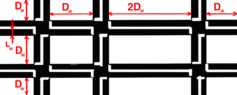
Figure 1: Urban road network. $L_{W}$ is the width of the lane, while the length of each road sector is an integer multiple of $D_{W}$.

Throughout the paper, $\mathbb{N}_{0}$ denotes the set of nonnegative integers, $\mathbb{R}$ the set of real numbers, and $\mathbb{N}$ the set of positive integers. The set of nonnegative and positive real numbers are, respectively, $\mathbb{R}_{\geq 0}$ and $\mathbb{R}_{>0}$. Given a set $\mathcal{S}$, its cardinality is $|\mathcal{S}|$. An undirected graph is a pair $(\mathcal{S},\mathcal{A})$, where $\mathcal{S}$ is a set of nodes and $\mathcal{A}\subseteq[\mathcal{S}]^{2}$ a set of arcs, with $[\mathcal{S}]^{2}$ denoting the set of all two-element subsets of $S$. Given a node $i\in\mathcal{S}$, its neighbors set is $\mathcal{S}_{i}=\{j\mid\{i,j\}\in\mathcal{A}\}$. A path between nodes $i_{1}\in\mathcal{S}$ and $i_{n}\in\mathcal{S}$ $i_{1}\not=i_{n}$, is a set of arcs of the form $\amalg=\{\{i_{1},i_{2}\},\{i_{2},i_{3}\},\dots\{i_{n-2},i_{n-1}\},\{i_{n-1},i_{n}\}\}$. The graph $(\mathcal{S},\mathcal{A})$ is connected if there exists a path between any pair of nodes $i,j$, $i\not=j$. It is fully connected, if there is an arc between any two nodes, i.e., $\mathcal{A}=[\mathcal{S}]^{2}$. The i-th entry of vector $\mathbf{v}$ is $(\mathbf{v})_{i}$. Two sorting functions are used. The function $\text{sort}:\mathbb{R}^{n}_{\geq 0}\rightarrow\mathbb{R}^{n}_{\geq 0}$ organizes vector elements in decreasing order of magnitude; the function $\text{argsort}:\mathbb{R}^{n}_{\geq 0}\rightarrow\mathbb{N}^{n}$ displays vector indices in decreasing order of their respective entries’ magnitude. The function $\text{argmax}:\mathbb{R}^{n}_{\geq 0}\rightarrow\mathbb{N}$ yields the index of the maximal entry in the vector. If more than one entry has maximum value, one index is selected randomly among the possible candidates.

II Problem Description

An urban road network is a system of interconnected roads which are designed to carry vehicular traffic, as in Figure 1. Each road is composed of two lanes, one per direction. For simplicity and without loss of generality, only a Manhattan-like grid, in which all roads are perpendicularly intersecting, will be analyzed. Overtaking and u-turns are forbidden. The traffic is composed of fully autonomous vehicles communicating with each other (V2V). The availability of a common shared clock is assumed.

II-A Vehicle model

A set $\mathbf{N}=\{1,\dots,n\}$ of $n>1$ vehicles driving on the urban road network is considered. Each vehicle, say $i\in\mathbf{N}$, is given a desired path in global coordinates, i.e. $\mathcal{P}_{i}=\{\mathbb{X}_{i}^{g},\mathbb{Y}_{i}^{g}\}\subset\mathbb{R}^{2}$, which comes from a higher-level GPS navigation system. The latter provides vehicle $i$ also with a desired cruising speed, i.e. $v_{i}^{r}\in\mathbb{R}_{>0}$. Each vehicle $i\in\mathbf{N}$ is modeled, as in [9], by a point-mass discrete-time linear system. Let $\mathbf{x}_{i}(k)=[p_{i}(k),v_{i}(k)]^{\prime}$ be its state vector, where $p_{i}(k)\in\mathbb{R}_{>0}$ and $v_{i}(k)\in\mathbb{R}_{\geq 0}$ are, respectively, position and velocity along $\mathcal{P}_{i}$ at discrete time instant $k\in\mathbb{N}_{0}$;

$$\mathbf{x}_{i}(k+1)=A\mathbf{x}_{i}(k)+Bu_{i}(k),$$ (1)

where

$$A=\begin{bmatrix}1&T_{s}\\ 0&1\end{bmatrix},\ B=\begin{bmatrix}0\\ T_{s}\end{bmatrix},$$ (2)

$T_{s}\in\mathbb{R}_{>0}$ is the sampling time, $\mathbf{x}_{i}(0)=\mathbf{x}_{i_{0}}$, and $u_{i}:\mathbb{N}\rightarrow\mathbb{R}$ is the longitudinal acceleration of vehicle $i$ along $\mathcal{P}_{i}$. In the following, we refer to $p_{i}$ as position in local coordinates. Each vehicle $i$ will have a local to global map $\mathcal{M}_{i}:\mathbb{R}_{\geq 0}\rightarrow\mathcal{P}_{i}$, which will associate $p_{i}$ to the respective position in the global frame, i.e.

$$\mathcal{M}_{i}(p_{i}(k))=\mathbf{x}_{i}^{g}(k)=(x_{i}^{g}(k),\ y_{i}^{g}(k))\in\mathcal{P}_{i}.$$ (3)

The global to local map is also defined and denoted by $\mathcal{M}_{i}^{-1}:\mathcal{P}_{i}\rightarrow\mathbb{R}_{\geq 0}$. Given two vehicles $i,j$ and a discrete-time index $k\in\mathbb{N}_{0}$, their distance is defined as

$$d_{i,j}^{k}=d(\mathbf{x}_{i}^{g}(k),\ \mathbf{x}_{j}^{g}(k))=\\ \sqrt{(x_{i}^{g}(k)-x_{j}^{g}(k))^{2}+(y_{i}^{g}(k)-y_{j}^{g}(k))^{2}}.$$ (4)

We say that, at time $k$, a collision between vehicle $i$ and $j$ occurs if $d_{i,j}^{k}<\underline{d}$, where $\underline{d}\in\mathbb{R}_{>0}$ is a given minimum allowed distance.

II-B Frontal Vehicles

Clearly, different vehicles can simultaneously drive along the same lane. It is important that each vehicle $i$ recognizes its current frontal vehicles, so that any possible bumper-to-bumper collision can be avoided. Let $\mathcal{F}_{i}^{k}$ be the set of $i$’s frontal vehicles at time $k$, formally

$$\mathcal{F}_{i}^{k}=\{j\in\mathbf{N}\mid\mathcal{M}_{j}(p_{j}(k))\in\mathcal{P}_{i},\\ \mathcal{M}_{i}^{-1}(\mathcal{M}_{j}(p_{j}(k)))>p_{i}(k)\}.$$ (5)

II-C Collision Points

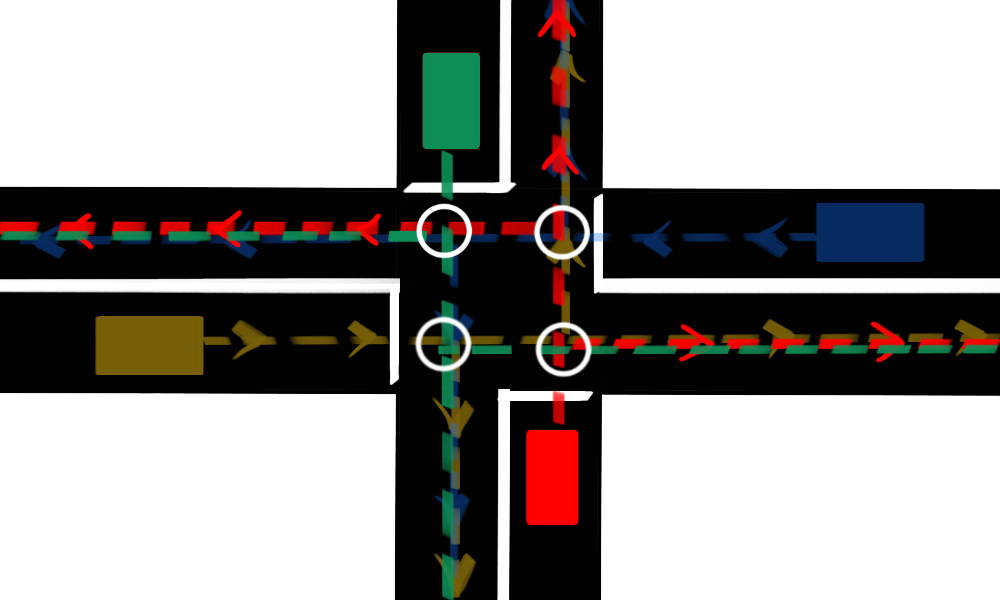
Figure 2: Possible collision points in one intersection.

Vehicle $i$ should be aware of all those vehicles driving on different road sections but going to intersect $\mathcal{P}_{i}$. All the possible paths, i.e. $\{\mathcal{P}_{i}\mid i\in\mathbf{N}\}$, will determine the set of all possible collision points in the network (cf. Figure 2),

$$\mathcal{H}=\{(h_{x},\ h_{y})\in\mathbb{R}^{2}\}.$$ (6)

Let $G_{i}^{k}$ be the set of all collision points that vehicle $i$ has still to cross at time $k$, i.e.

$$G_{i}^{k}=\{h\in\mathcal{H}\mid h\in\mathcal{P}_{i},\ \mathcal{M}_{i}^{-1}(h)>p_{i}(k)\}.$$ (7)

On the other hand, given $h\in\mathcal{H}$, the set $H_{h}^{k}$ collects all the vehicles that still have to cross, at time $k$, the collision point $h$, i.e.,

$$H_{h}^{k}=\{i\in\mathbf{N}\mid h\in\mathcal{H},\ h\in\mathcal{P}_{i},\ \mathcal{M}_{i}^{-1}(h)>p_{i}(k)\}.$$ (8)

Let $\mathcal{L}_{i}^{k}$ be the set of all vehicles with a higher priority than vehicle $i$ for crossing the collision point in $G_{i}^{k}$. A method to compute $\mathcal{L}_{i}^{k}$ in a complete decentralized fashion will be presented in Section III.

II-D Control Structure

Figure 3: Hierarchical control structure for vehicle $i$.

This information plays a rucial role within the hierarchically structured controller for vehicle $i$ (see Figure 3). The ingredients of this controller are described below:

Reference Generator

Its task is providing the on-board controller with the desired path and cruising speed, given the goal position. It is outside the scope of this paper.

CBAA-M

this layer runs the so-called Consensus-based Auction Algorithm Modified (see Section III). Vehicle $i$ will run this algorithm at every discrete-time step $k$ thus providing the controller with the set $\mathcal{L}_{i}^{k}$ of higher priority vehicles, introduced in Section II-C.

MPC

this on-board Model Predictive Controller minimizes a cost function (reflecting deviations from the desired speed, discomfort, etc) while avoiding collisions with vehicles in set $\mathcal{F}_{i}^{k}\cup\mathcal{L}_{i}^{k}$. Its output is the acceleration $u_{i}(k)$.

The proposed structure builds on the idea of avoiding collisions only with higher priority and frontal vehicles, which was originally proposed in [8].

III Consensus-based Auction Algorithm Modified

CBAA-M is an algorithm that allows a multi-agent system modeled by a graph $(\mathcal{S},\mathcal{A})$ to achieve an agreement between a set of agents. of agents. It has been presented in [5], which, in turn, takes inspiration from [6]. This algorithm is able to run an auction without requiring the presence of any central auctioneer. It can therefore be employed in a completely decentralized control approach, as the one adopted in our strategy. In the following, we will briefly summarize CBAA-M and prove that it converges for connected graphs. This is a sharper result than in [5], where full connectedness was assumed.

Each agent $i\in\mathcal{S}=\{1,\dots,S\}$ places a bid $c_{i}\in\mathbb{R}_{>0}$ that determines its position in the sequence. We assume that each agent has a distinct bid to place, i.e. $\forall i\not=j,\ c_{i}\not=c_{j}$. The higher the bid, the earlier that agent could appear in the resulting sequence. Each agent has two vectors of dimension $S$, i.e. $\mathbf{v}_{i}$ and $\mathbf{w}_{i}$, which are updated at each iteration $\kappa\in\mathbb{N}$ and are initialized as zero vectors. The first vector (winners list) has to be filled with a sequence of agents’ indexes, whilst the second vector contains their respective bids. This algorithm is composed of two subsequent phases within every iteration step $k$:

• Local Auction [Algorithm 1]: at each iteration $\kappa$, each agent $i\in\mathcal{S}$ places, if its index is not already stored in $\mathbf{v}_{i}^{\kappa}$, its own bid $c_{i}$ in the earliest possible position of vector $\mathbf{w}_{i}^{\kappa}$. In the same position, it stores its index in vector $\mathbf{v}_{i}^{\kappa}$.

Algorithm 1 CBAA-M Phase 1 for agent $i$ at iteration $\kappa$

1:$\mathbf{v}_{i}^{0}=\mathbf{0}_{S}$ , $\mathbf{w}_{i}^{0}=\mathbf{0}_{S}$

2:procedure Bid($c_{i}$, $\mathbf{v}_{i}^{\kappa-1}$, $\mathbf{w}_{i}^{\kappa-1}$)

3:     $\mathbf{v}_{i}^{\kappa}\leftarrow\mathbf{v}_{i}^{\kappa-1}$

4:     $\mathbf{w}_{i}^{\kappa}\leftarrow\mathbf{w}_{i}^{\kappa-1}$

5:     $j\leftarrow 1$

6:     loop:

7:     if $i\not=(\mathbf{v}_{i}^{\kappa})_{l}$, $\forall l=1\dots S$ then

8:         if $c_{i}>(\mathbf{w}_{i}^{\kappa-1})_{j}$ then

9:              $(\mathbf{v}_{i}^{\kappa})_{j}\leftarrow i$

10:              $(\mathbf{w}_{i}^{\kappa})_{j}\leftarrow c_{i}$          

11:         $j\leftarrow j+1$

12:         goto loop.      

13:     close;

• Consensus over the lists [Algorithm 2]: after the first phase, each agent has its own version of $\mathbf{v}_{i}^{\kappa}$ and $\mathbf{w}_{i}^{\kappa}$. The network need to reach an agreement on them. For that purpose, each agent $i\in\mathcal{S}$ sends its vectors to its respective neighbors (i.e. the nodes in the set $\mathcal{S}_{i}$) and receives theirs. Then, via a max-consensus protocol, it selects the best bid for each row of $\mathbf{w}_{i}^{\kappa}$ and puts in the same position of $\mathbf{v}_{i}^{\kappa}$ the respective agent’s index.

Algorithm 2 CBAA-M Phase 2 for agent $i$ at iteration $\kappa$

1:SEND $(\mathbf{v}_{i}^{\kappa},\mathbf{w}_{i}^{\kappa})$ to $j\in{\mathcal{S}}_{i}=\{j\in\mathcal{S}\mid(i,j)\in\mathcal{E}\}$

2:RECEIVE $(\mathbf{v}_{h}^{\kappa},\mathbf{w}_{h}^{\kappa})$ from $h\in{{\mathcal{S}}}_{i}=\{j\in\mathcal{S}\mid(j,i)\in\mathcal{E}\}$

3:procedure Update($\mathbf{v}_{h\in{\mathcal{S}}_{i}}^{\kappa}$, $\mathbf{w}_{h\in{\mathcal{S}}_{i}}^{\kappa}$)

4:     $(\mathbf{{a}}_{i}^{\kappa})_{j}\leftarrow\operatorname*{arg\,max}\limits_{h\in\mathcal{S}_{i}}((\mathbf{w}_{h}^{\kappa})_{j}),\ \forall j=1\dots\max(\kappa,S)$

5:     $(\mathbf{v}_{i}^{\kappa})_{j}\leftarrow(\mathbf{v}_{(\mathbf{{a}}_{i}^{\kappa})_{j}}^{\kappa})_{j}\quad\forall j=1\dots\max(\kappa,S)$

6:     $(\mathbf{w}_{i}^{\kappa})_{j}\leftarrow\max\limits_{h\in\mathcal{S}_{i}}((\mathbf{w}_{h}^{\kappa})_{j})\quad\forall j=1\dots\max(\kappa,S)$

After terminating Phase 2, $(\mathbf{w}_{h}^{\kappa})_{j}$ is the maximal bid for position $j$ that agent $i$ is aware of, and $(\mathbf{v}_{h}^{\kappa})_{j}$ is the index of the agent having placed that bid.

In [5], a fully connected network topology was assumed and an agreement was shown to be reached in exactly $S$ iterations. In the following, we will show that the algorithm converges under the weaker condition of $(\mathcal{S},\mathcal{A})$ being connected.

Proposition 1.

A multi-agent system represented by a connected graph $(\mathcal{S},\mathcal{A})$ executes CBAA-M. An agreement is reached in $\bar{\kappa}\in\mathbb{N}$ iterations. Formally, $\exists\bar{\kappa}\in\mathbb{N}$:

$$\forall i,j\in\mathbb{N},\ \ \ \mathbf{v}_{i}^{\bar{\kappa}}=\mathbf{v}_{j}^{\bar{\kappa}}=\mathbf{v}^{*}=\text{argsort}(\mathbf{c}),$$ (9)

$$\mathbf{w}_{i}^{\bar{\kappa}}=\mathbf{w}_{j}^{\bar{\kappa}}=\mathbf{w}^{*}=\text{sort}(\mathbf{c}),$$ (10)

where, $\forall i\in\mathcal{S},\ (\mathbf{c})_{i}=c_{i}$.

Proof.

Given a pair $i\in\mathcal{S},\ \kappa\in\mathbb{N}$, such that $\mathbf{v}_{i}^{\kappa}=\mathbf{v}^{*}$ and $\mathbf{w}_{i}^{\kappa}=\mathbf{w}^{*}$, the following holds:

$$\forall j\in\mathcal{S}_{i}\cup\{i\},\ \mathbf{v}_{j}^{\kappa+1}=\mathbf{v}^{*},\ \mathbf{w}_{j}^{\kappa+1}=\mathbf{w}^{*}.$$ (11)

In fact, if (11) does not hold, Algorithm 2 would imply that, for an arbitrary $j\in\mathcal{S}_{i}$, $\exists g=1,\dots,S,\ (\mathbf{w}_{j}^{\kappa})_{g}>(\mathbf{w}^{*})_{g}$. The latter, by Algorithm 1, means that $\exists h=1,\dots,S:\ c_{g}<{c}_{h}<c_{g+1}$, which is in contradiction with the definition of $\mathbf{w}^{*}$, i.e. $\mathbf{w}^{*}=\text{sort}(\mathbf{c})$. A similar analysis can be conducted for $\mathbf{v}_{j}^{\kappa}$.

The agreement phase of CBAA-M follows a max-consensus protocol for each row of $\mathbf{v}_{i}$ and $\mathbf{w}_{i}$. By [10], max-consensus is achieved in a connected network in at most $l$ steps, where

$$l=\max_{i,j\in\mathcal{S}}\{|i,j|_{l,min}\},$$ (12)

where $|i,j|_{l,min}$ denotes the length of the shortest existing path between node $i$ and node $j$. Therefore, by (11) and (12), if agent $i_{0}$ at iteration $\kappa_{0}$ is the first agent to have $\mathbf{v}_{i_{0}}^{\kappa_{0}}=\mathbf{v}^{*}$ and $\mathbf{w}_{i_{0}}^{\kappa_{0}}=\mathbf{w}^{*}$, then $\bar{\kappa}\leq\kappa_{0}+l$.

Let’s now estimate $\kappa_{0}$ in the worst case scenario. By Algorithm 1, intuitively, ${i}_{0}$ is the first agent to fill the last row of $\mathbf{w}_{i}$. This is only possible, by Algorithm 1, if $i_{0}$ is not contained in $\mathbf{v}_{i}$ and if the first $S-1$ rows of $\mathbf{w}_{i}$ have already been filled. By this, agent $i_{0}$ must be the agent having the minimum bid in the network, i.e. $c_{{i}_{0}}=\min_{i\in\mathcal{S}}c_{i}$. In the worst case scenario, by [10] and (12), for retrieving the information of each row $j$ of $\mathbf{v}_{i}$ and $\mathbf{w}_{i}$, agent $i$ needs maximum $l$ steps. Therefore, always in the worst case scenario, $\kappa_{0}\leq(S-1)l$. Finally, we can state that the multi-agent system achieves an agreement as (9)-(10) in $\bar{\kappa}$ steps, where

$$\bar{\kappa}\leq\kappa_{0}+l\leq(S-1)l+l=Sl.$$

This concludes the proof. ∎∎

Due to the need of real-time implementation, a fast convergence to the agreement vector is often required. In [11], it was shown how the convergence rate of a max-consensus protocol can be drastically increased by harnessing the interference

As claimed in Section II-D, each vehicle $i\in\mathbf{N}$, at every discrete time step $k\in\mathbb{N}_{0}$, runs one CBAA-M for each collision point $h\in G_{i}^{k}$, thus retrieving $|G_{i}^{k}|$ priority vectors. These can be grouped in a set $\{\mathbf{v}_{h}^{*}\mid h\in G_{i}^{k}\}$, where $\mathbf{v}_{h}^{*}\in\mathbb{N}^{|H_{h}^{k}|}$ is the agreed crossing priority list for collision point $h$. From this collection of vectors, vehicle $i$ can retrieve the set $\mathcal{L}_{i}^{k}$ (cf. Section II-C) that collects all the vehicles having higher priority than $i$ at some collision points. Formally,

$$\mathcal{L}_{i}^{k}=\{(\mathbf{v}_{h}^{*})_{j}\mid h\in G_{i}^{k},\ j<m,\ (\mathbf{v}_{h}^{*})_{m}=i\}.$$ (13)

As in [5], the bid $c_{i,h}^{k}$ placed by vehicle $i$ at time $k$ in the auction for crossing $h\in G_{i}^{k}$ is determined from its current velocity and its distance from $h$:

$$c_{i,h}^{k}=\frac{p_{v}v_{i}(k)+p_{d}}{d_{i,h}^{k}+\epsilon},$$ (14)

where $p_{v}\in\mathbb{R}_{>0}$, $p_{d}\in\mathbb{R}_{>0}$, and $\epsilon\in\mathbb{R}_{>0}$ are chosen parameters (equal for all vehicles). The quantity $d_{i,h}^{k}$ is the distance at time $k$ from vehicle $i$ to the collision point $h\in\mathcal{H}$, i.e., $d_{i,h}^{k}=\sqrt{(x_{i}^{g}(k)-h_{x})^{2}+(y_{i}^{g}(k)-h_{y})^{2}}$. The reader can refer to [5] for a comprehensive analysis of $c_{i,h}^{k}$ and potential coherency problems in the auction procedures.

IV Onboard Model Predictive Controller

As shown in Figure 3, each vehicle $i\in\mathbf{N}$ has an on-board MPC controller that computes an optimal longitudinal acceleration at every discrete step $k\in\mathbb{N}_{0}$. It is provided with the desired path $\mathcal{P}_{i}$, the desired cruising speed $v_{i}^{r}$, the current vehicle state $\mathbf{x}_{i}(k)$, the sets $\mathcal{L}_{i}^{k}$ and $\mathcal{F}_{i}^{k}$, and the states $\mathbf{x}_{j}(k)$ of all vehicles $j\in\mathcal{L}_{i}^{k}\cup\mathcal{F}_{i}^{k}$.

IV-A Prediction Model

MPC employs a prediction model of the traffic situation extrapolated from the current states and evolving along a horizon $T_{h}\in\mathbb{N}$. In the following, we describe the optimal control problem to be solved at every $k\in\mathbb{N}_{0}$ by vehicle $i\in\mathbf{N}$.

The predicted state and input of vehicle $i$ itself are $\tilde{\mathbf{x}}_{i}(t)=[\tilde{p}_{i}(t),\tilde{v}_{i}(t)]$ and $\tilde{u}_{i}(t),\ t\in[0,T_{h}]$. The prediction model evolves according to

$$\tilde{\mathbf{x}}_{i}(t+1)=A\tilde{\mathbf{x}}_{i}(t)+B\tilde{u}_{i}(t),$$ (15)

where $t\in[0,T_{h}-1]$. The prediction model of other vehicles is based on a constant acceleration assumption: in fact, $\forall\zeta\in\mathcal{F}_{i}^{k}\cup\mathcal{L}_{i}^{k}$,

$$\tilde{\mathbf{x}}_{\zeta}(t+1)=A\tilde{\mathbf{x}}_{\zeta}(t)+B\tilde{u}_{\zeta},$$ (16)

where $t\in[0,T_{h}-1]$ and $\tilde{u}_{\zeta}=u_{\zeta}(k)$. Clearly, the prediction variables are initialized according to the current measurement at instant $k$, i.e.,

$$\tilde{\mathbf{x}}_{i}(0)=\mathbf{x}_{i}(k),$$ (17)

$$\forall\zeta\in\mathcal{L}_{i}^{k}\cup\mathcal{F}_{i}^{k},\ \tilde{\mathbf{x}}_{\zeta}(0)=\mathbf{x}_{\zeta}(k).$$ (18)

Remark 1.

Let $\mathcal{F}_{i}^{t},\ \forall t\in[0,T_{h}]$, be the set of vehicles $j\in\mathcal{L}_{i}^{k}\cup\mathcal{F}_{i}^{k}$ that are in front of vehicle $i$ at prediction time $t$. Formally, as in (5),

$$\mathcal{F}_{i}^{t}=\{j\in\mathcal{L}_{i}^{k}\cup\mathcal{F}_{i}^{k}\mid\mathcal{M}_{j}(\tilde{p}_{j}(t))\in\mathcal{P}_{i},\\ \mathcal{M}_{i}^{-1}(\mathcal{M}_{j}(\tilde{p}_{j}(t)))\geq\tilde{p}_{i}(t)\}.$$ (19)

Since any vehicle in $\mathcal{L}_{i}^{k}\cup\mathcal{F}_{i}^{k}$ always has priority in front of $i$, requiring $\mathcal{M}_{i}^{-1}(\mathcal{M}_{j}(\tilde{p}_{j}(t)))\geq\tilde{p}_{i}(t)$ in (19) is redundant. Accordingly, (19) can be rewritten as

$$\mathcal{F}_{i}^{t}=\{j\in\mathcal{L}_{i}^{k}\cup\mathcal{F}_{i}^{k}\mid\mathcal{M}_{j}(\tilde{p}_{j}(t))\in\mathcal{P}_{i}\},$$ (20)

thus making it clear that the usage of $\mathcal{F}_{i}^{t}$ does not affect the convexity of the problem, since it does not depend on the choice of $\tilde{u}_{i}(t)$.

IV-B Obstacle Avoidance

We employ, similarly to [8], the idea of avoiding collisions with higher priority and frontal vehicles. The safety distance to be kept is defined via the continuous-time headway rule, as in [12]. Then, a general collision avoidance constraint between vehicle $i$ and an arbitrary vehicle $\zeta$ at prediction time $t$ is of the form

$$d(\tilde{\mathbf{x}}_{i}^{g}(t),\tilde{\mathbf{x}}_{\zeta}^{g}(t))\geq\lambda\tilde{v}_{i}(t)+\underline{d}+\delta(t),$$ (21)

where $\lambda$ is the so called time-headway (measured in seconds) and $\underline{d}$ is the fixed bumper-to-bumper distance defined in Section II-A. The remaining term, $\delta(t)$, is a slack variable that will be weighted in the cost function and that is traditionally used in the formulation of soft constraints. This allows the optimal controller to increase, if possible, the safety distance. In Section IV-C, $\delta(t)$ will be constrained to a given set.

Clearly, having $d(\tilde{\mathbf{x}}_{i}^{g}(t),\tilde{\mathbf{x}}_{\zeta}^{g}(t))$ formulated as in (4) makes the problem non-convex. In order to prevent this, in [5], collision avoidance constraints were reformulated. By [5, Proposition 3], constraints to avoid collisions with frontal vehicles can be rewritten as

$$\forall t\in[0,T_{h}],\ \forall\zeta\in\mathcal{F}_{i}^{t},\\ \mathcal{M}_{i}^{-1}(\mathcal{M}_{\zeta}(\tilde{p}_{\zeta}(t)))-\tilde{p}_{i}(t)\geq\lambda\tilde{v}_{i}(t)+\underline{d}+\delta(t).$$ (22)

Clearly, (22) is convex.

In [5], left turns are disallowed, since allowing left turns is claimed to lower traffic efficiency. In this paper, we do allow left turns at intersections and analyze the effect of this in Section 8. First, we introduce a general convex collision avoidance constraint for vehicle $i$ and all higher priority vehicles crossing $\mathcal{P}_{i}$ i.e. $\zeta\in\mathcal{L}_{i}^{k}\setminus\mathcal{F}_{i}^{k}$. The following proposition extends the outcome of [5, Proposition 4].

Proposition 2.

Given a vehicle $\zeta\in\mathcal{L}_{i}^{k}\setminus\mathcal{F}_{i}^{k}$, the constraint, $\forall h\in G_{i}^{k}\cap G_{\zeta}^{k}$:

$$\mathcal{M}_{i}^{-1}(h)-\tilde{p}_{i}(t)\geq\lambda\tilde{v}_{i}(t)+\underline{d}+\delta(t),\\ \forall t\in[0,T_{h}]:\ \zeta\not\in\mathcal{F}_{i}^{t}\land\mathcal{M}_{\zeta}^{-1}(h)-\tilde{p}_{\zeta}(t)\geq-\underline{d},$$ (23)

guarantees that any collision between $i$ and $\zeta$ throughout the prediction horizon is avoided.

Proof.

A collision between $i$ and $\zeta$ occurs at prediction time $t$ if, as in Section II-A,

$$d(\mathbf{x}_{i}^{g}(t),\ \mathbf{x}_{\zeta}^{g}(t))\leq\underline{d}.$$ (24)

We can distinguish three different cases. (i) In the case $\zeta\in\mathcal{F}_{i}^{t}$, any collision is avoided if (22) holds. (ii) if $\zeta\not\in\mathcal{F}_{i}^{t}$, but $\mathcal{M}_{\zeta}^{-1}(h)-\tilde{p}_{\zeta}(t)<-\underline{d}$, vehicle $\zeta$ at prediction time $t$ does not lie on $\mathcal{P}_{i}$ and has driven at a distance larger than $\underline{d}$ far from $\mathcal{P}_{i}$, (24) does not hold. (iii) as long as $\zeta\not\in\mathcal{F}_{i}^{t}\land\mathcal{M}_{\zeta}^{-1}(h)-\tilde{p}_{\zeta}(t)\geq-\underline{d}$, the distance between $i$ and $\mathcal{P}_{\zeta}$ is larger than $\lambda\tilde{v}_{i}(t)+\underline{d}+\delta(t)$, which is clearly larger than $\underline{d}$. This concludes the proof. ∎∎

The resulting convex collision avoidance constraint then becomes:

$$\forall h\in G_{i}^{k}\cap G_{\zeta}^{k},\ \mathcal{M}_{i}^{-1}(h)-\tilde{p}_{i}(t)\geq\lambda\tilde{v}_{i}(t)+\underline{d}+\delta(t),\\ \forall t\in[0,T_{h}]:\ \zeta\not\in\mathcal{F}_{i}^{t}\land\mathcal{M}_{\zeta}^{-1}(h)-\tilde{p}_{\zeta}(t)\geq-\underline{d}.$$ (25)

IV-C Other Constraints and Cost Function

Traditional constraints on the allowed speed and acceleration can be formulated as follows:

$$\forall t\in[0,T_{h}],\ \tilde{u}_{i}(t)\in[\underline{a}_{i},\bar{a}_{i}],$$ (26)

$$\tilde{v}_{i}(t)\in[\underline{v},\bar{v}],$$ (27)

$$\tilde{v}_{\zeta}(t)\in[\underline{v},\bar{v}],$$ (28)

where $\underline{v}>0$, thus guaranteeing that vehicles do not drive backwards.

The slack variable $\delta(t)$ is also constrained to a given set, i.e.

$$\forall t\in[0,T_{h}],\ \delta(t)\in[-\bar{\lambda}\tilde{v}_{i}(t),\bar{\delta}],$$ (29)

where $0\leq\bar{\lambda}<\lambda$ and $\bar{\delta}>0$. By this, the time headway in (21) can be diminished down to $\lambda-\bar{\lambda}$, although this will be negatively weighted in the cost function, thus aiming to increase the safety distance.

The controller performance can be evaluated by the following cost function

$$J=\sum_{t=0}^{T_{h}}q(\tilde{v}_{i}(t)-v_{i}^{r})^{2}+r\tilde{u}_{i}^{2}(t)+\omega\delta(t),$$ (30)

where $q,r\in\mathbb{R}_{>0}$ and $\omega\in\mathbb{R}_{<0}$ are design parameters. The first term of the sum punishes deviations from the desired speed $v_{i}^{r}$; the second term discourages high values of acceleration or deceleration, thus pledging a better comfort on-board. The last term punishes small $\delta(t)$, hence contributing to crease safety.

The optimal control problem is then formulated as follows:

$$\min\limits_{\tilde{u}_{i}(0)\dots\tilde{u}_{i}(T_{h})}\ \ \$$ cost function (30)

s.t. Prediction model (15-18)

Safety constraints (22, 25)

$$\text{Input and state constraints (\ref{eq:classicConstr1}- \ref{eq:constrainedDelta})}.$$

A vector of inputs composed of $\tilde{u}_{i}(0)\dots\tilde{u}_{i}(T_{h})$ will solve the optimal control problem. Coherently with the MPC structure, only the first optimal control input will be executed in (1) at each $k\in\mathbb{N}$, i.e. $u_{i}(k)=\tilde{u}_{i}(0)$.

V Simulation

TABLE I: Problem data.

$L_{w}=3.5m$, $D_{w}=30m$, $T_{s}=0.25s$, $p_{c}=1$, $p_{d}=0.1$, $\epsilon=0.1$

$\lambda=1s$, $\bar{\lambda}=0.5s$, $\bar{\delta}=10m$, $\underline{d}=2.1m$, $\underline{v}=0$, $\bar{v}=130km/h$,

$T_{h}=10$, $\underline{a}_{i}=-9m/s^{2}$, $\bar{a}_{i}=5m/s^{2}$, $q=0.1$, $r=0.01$, $\omega=-0.1$

$v_{min}=52km/h$, $v_{max}=56km/h$, $\wp=0.5$

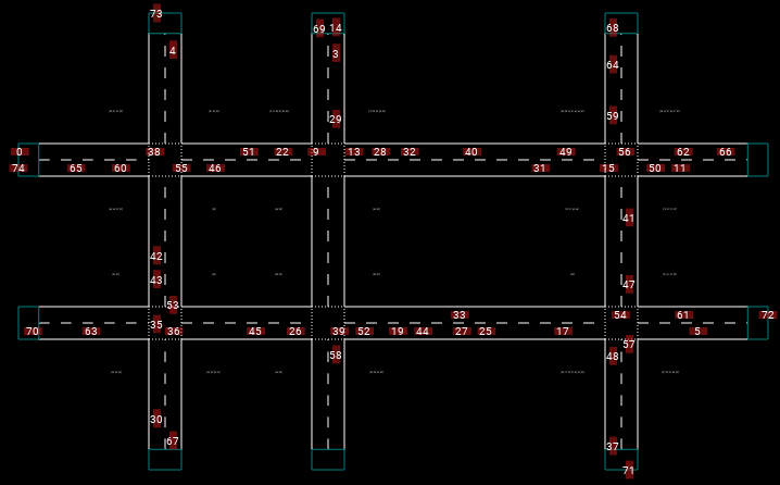
Figure 4: Using the open-source software YatSim for modeling the urban road network.

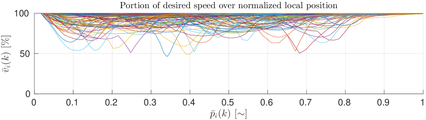
(a) Vehicles’ speed ratios over normalized local coordinate.

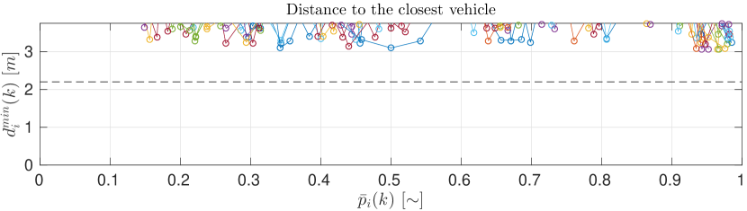
(b) Vehicles’ minimum distance over normalized local coordinate.

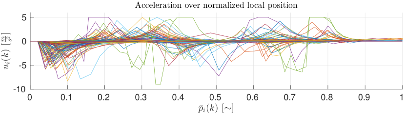
(c) Vehicles’ accelerations over normalized local coordinate. The dashed line indicates the minimum allowed distance,

Figure 5: Analysis of individual vehicles’ characteristics.

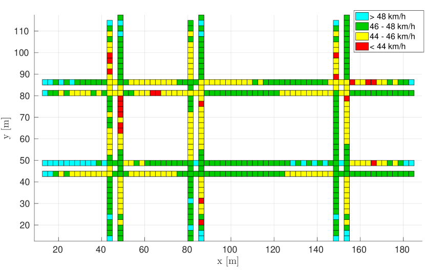
(a) Macroscopic analysis of the average speed in road network sections.

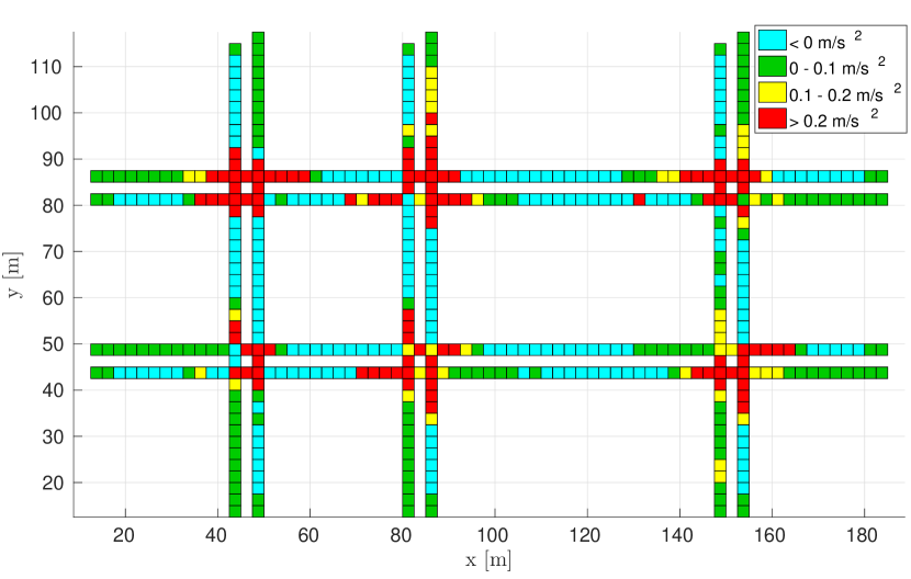
(b) Macroscopic analysis of the average acceleration in road network sections.

Figure 6: Macroscopic analysis.

The traffic flowing in the urban road network sketched in Figure 1 can be simulated by means of the open-source programme YatSim [13], as in Figure 4. Vehicles will employ the decentralized control strategy presented in this paper. In the following, a macroscopic analysis of the traffic (in the sense of [14]) will be conducted. Accordingly, the traffic will be studied as a flow. This allows to quantify the impact that this control strategy has on the urban road network as a whole, hopefully resulting in an improvement of flow performance indexes, such as average or minimum speed and acceleration.

V-A Macroscopic Analysis

Vehicles will be randomly injected into the network; at each discrete time step from each road, provided that there is enough space to avoid trivial initial collisions, a vehicle, say $i\in\mathbf{N}$, will enter the road network with a given probability $\wp\in(0,1)$. Its desired speed $v_{i}^{r}$ will be drawn out of an uniform distribution $\mathcal{U}_{[v_{min},v_{max}]}$. Also its desired path $\mathcal{P}_{i}$ will be chosen in a random way, as illustrated in [13]. The parameters used for the simulation are contained in Table I. The simulation is run until more than $500$ vehicles complete their paths. For what concerning simulation results, the average speed of the traffic is $46.8[\frac{km}{h}]$, which, by [15], is much higher than the current average traffic speed in New York City ($28.32[\frac{km}{h}]$) or Boston ($33.64[\frac{km}{h}]$). We use these two cities as benchmark, since the road network structure composed of perpendicularly intersecting streets is similar to the one considered here. Moreover, $\wp$ has been chosen to replicate real congestion conditions. Vehicles are injected in the simulation environment with their desired speeds. Intuitively, they will have to slow down in order to avoid collisions. In fact, the average acceleration of the traffic is $-0.0212[\frac{m}{s^{2}}]$, thus showing a breaking behavior.

Given a vehicle $i\in\mathbf{N}$, let $\bar{p}_{i}(k)$ be its normalized local coordinate, i.e. $\forall k\in\mathbb{N}$,

$$\bar{p}_{i}(k)=\frac{p_{i}(k)}{\max\limits_{k}p_{i}(k)}\in[0,1],$$

let $\bar{v}_{i}(k)$ be its speed ratio, i.e. $\forall k\in\mathbb{N}$,

$$\bar{v}_{i}(k)=\frac{v_{i}(k)}{v_{i}^{r}}100\%,$$

and let $d_{i}^{min}(k)$ be the minimum distance towards other vehicles at instant $k$, i.e. $\forall k\in\mathbb{N}$,

$${d}_{i}^{min}(k)=\min\limits_{j\in\mathbb{N}\setminus\{i\}}d_{ij}(k).$$

Although this section presents a macroscopic analysis, a detailed evaluation of individual vehicles’ characteristics is also reviewed. Figure 5(a) shows the evolution of speed ratios as function of normalized local coordinates for each individual vehicle. The large majority of vehicles keep a speed above the $80\%$ of their desired ones, while no vehicle is slowing down below the $48\%$ of its desired speed. By comparing this result to the traditional solution with traffic lights, the improvement is explicit since no vehicle is actually stopping. This might intuitively result in decreasing the traffic safety (which can be defined as the likelihood of having collisions). However, Figure 5(b) shows that all vehicles keep a safety distance larger than $\underline{d}$. Moreover, the amount of vehicles getting close to this minimum allowed value is marginal. Figure 5(c) outlines individual vehicles’ accelerations as function of $\bar{p}_{i}(k)$. As already motivated above, many vehicles brake as soon as they enter the simulation environment. Vehicles are often saturating their acceleration, in those cases when collision avoidance constraints allow to do so (e.g. as soon as that vehicle wins the decentralized auction). This saturating behavior can be intuitively mitigated by increasing $r$. Only in one point (e.g., for $p_{i}(k)$ between $0.3$ and $0.4$), a vehicle is saturating the braking power. This could be prevented by increasing $T_{h}$, length of the prediction horizon, or $\omega$, weight of the hold safety distance.

An analysis of which portions of the urban road network suffer the most of speed drops or robust braking is presented. First, the road network has to be divided into small fragments (e.g. squares of side $2.5[m]$) on which we compute the average characteristics of the traffic. As in Figure 6(a), average speeds lower than $44[\frac{km}{h}]$ are met in some roads entering an intersection (e.g. $(x=50,y=77.5)$ or $(x=155,y=77.5)$), while, along those roads leaving an intersection, higher speeds are found. Figure 6(b) shows that traffic along roads entering an intersection exhibits a braking behavior. On the other hand, vehicles try to leave the intersection as soon as possible once inside of it, thus resulting in higher average acceleration.

V-B Impact of Left-Turns

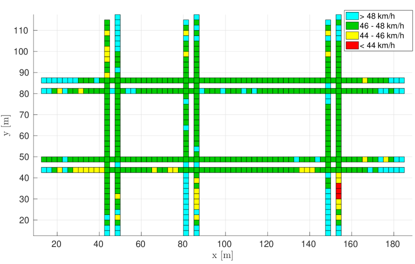
Figure 7: Macroscopic analysis of the average speed in road network sections. Left-turnings disallowed.

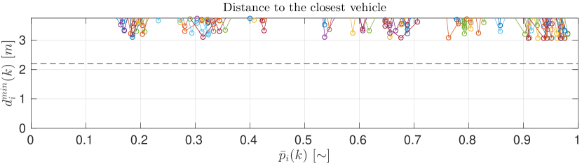
Figure 8: Vehicles’ minimum distance over normalized local coordinate. Left turnings disallowed. The dashed line indicates the minimum allowed distance,

In [5], left turnings were forbidden. Also, [16] revealed that a world-wide known delivery company has historically prohibited left-turnings to its drivers. This was due to the assumption that allowing left-turns affects traffic efficiency in a negative way and increases hazards. In the following, we repeat our simulation for the case when left-turns are forbidden. We simulate the same urban road network where cars have the same parameters (same initial and goal position) and are generated according to the same probability $\wp$; however, left turnings are in this case not allowed. The average speed of the traffic is $47.8[\frac{km}{h}]$ and the average acceleration is $-0.002[\frac{m}{s^{2}}]$. Additionally, Figure 7 shows that in almost all the portions composing the road network, vehicles keep a higher speed than in Figure 6(a). With regards to the outcome of the previous section, it is therefore clear that preventing vehicles from turning left increases the average speed and decreases their absolute acceleration. If the average speed is a measure of traffic efficiency, then the assumption presented by [16] seems reasonable.

On the other hand, under a safety-related point of view, we do not get to the same conclusion. Let us pick, as safety index, the minimum distance that each vehicle keeps towards the others, and let this be plotted, as function of the normalized local coordinates, in Figure 8. Its outcome is not much different than what Figure 5(b) yields. Therefore, left-turnings do not seem to increase hazards in the autonomous road traffic. One can guess that, although the overall average speed is affected by the presence of a left-turning traffic, safety is anyhow guaranteed by the presence of the on-board MPC controller.

VI Conclusion

In this paper, we suggested the use of a decentralized control scheme for vehicles in a urban traffic network. This scheme is based on a consensus-based protocol (CBAA-M), which gives vehicles crossing orders at the intersections, with an on-board MPC controller, responsible for avoiding collisions and tracking some performance. CBAA-M has been here proven to achieve an agreement in cases when the network topology is connected. This is in contrast to [5], where full connectedness was required. Finally, the impact of disallowing left-turning has been analyzed.

Future work will focus on real-time implementability issues by improving the convergence rate of the consensus protocol and decrease the complexity of the on-board MPC.

References

- [1] P. A. Ioannou and C.-C. Chien, “Autonomous intelligent cruise control,” IEEE Transactions on Vehicular technology, vol. 42, no. 4, pp. 657–672, 1993.
- [2] A. Katriniok, J. P. Maschuw, F. Christen, L. Eckstein, and D. Abel, “Optimal vehicle dynamics control for combined longitudinal and lateral autonomous vehicle guidance,” in European Control Conference (ECC). IEEE, 2013, pp. 974–979.
- [3] S. A. Arogeti and N. Berman, “Path following of autonomous vehicles in the presence of sliding effects,” IEEE Transactions on Vehicular Technology, vol. 61, no. 4, pp. 1481–1492, 2012.
- [4] F. Molinari, N. N. Anh, and L. Del Re, “Efficient mixed integer programming for autonomous overtaking,” American Control Conference (ACC), 2017, pp. 2303–2308, 2017.
- [5] F. Molinari and J. Raisch, “Automation of road intersections using consensus-based auction algorithms,” American Control Conference (ACC), pp. 5994 – 6001, 2018.
- [6] H.-L. Choi, L. Brunet, and J. P. How, “Consensus-based decentralized auctions for robust task allocation,” IEEE transactions on robotics, vol. 25, no. 4, pp. 912–926, 2009.
- [7] W. Ren, R. W. Beard, and E. M. Atkins, “Information consensus in multivehicle cooperative control,” IEEE Control Systems, vol. 27, no. 2, pp. 71–82, 2007.
- [8] A. Katriniok, P. Kleibaum, and M. Joševski, “Distributed model predictive control for intersection automation using a parallelized optimization approach,” IFAC-PapersOnLine, vol. 50, no. 1, pp. 5940–5946, 2017.
- [9] N. Murgovski, G. R. de Campos, and J. Sjöberg, “Convex modeling of conflict resolution at traffic intersections,” in Decision and Control (CDC), 2015 IEEE 54th Annual Conference on. IEEE, 2015, pp. 4708–4713.
- [10] B. M. Nejad, S. A. Attia, and J. Raisch, “Max-consensus in a max-plus algebraic setting: The case of fixed communication topologies,” in Information, Communication and Automation Technologies, 2009. ICAT 2009. XXII International Symposium on. IEEE, 2009, pp. 1–7.
- [11] F. Molinari, S. Stańczak, and J. Raisch, “Exploiting the superposition property of wireless communication for max-consensus problems in multi-agent systems,” 7th IFAC Workshop on Distributed Estimation and Control in Networked Systems (NecSys18), 2018.
- [12] C. Chien and P. Ioannou, “Automatic vehicle-following,” in American Control Conference, 1992. IEEE, 1992, pp. 1748–1752.
- [13] A. M. Dethof and F. Molinari, “Yatsim: an open-source simulator for testing consensus-based control strategies in urban traffic networks,” arXiv preprint arXiv:1810.11380, 2018.
- [14] A. D. May, Traffic flow fundamentals, 1990.
- [15] J. Kleint. (2009) Cityspeed at sourceforge. [Online]. Available: http://sourceforge.net/projects/cityspeed/
- [16] A. A. Reich, “Transportation efficiency,” Strategic Planning for Energy and the Environment, vol. 32, no. 2, pp. 32–43, 2012.