Ground and excited energy levels can be extracted exactly from a single ensemble density-functional theory calculation

Abstract

Gross–Oliveira–Kohn density-functional theory (GOK-DFT) for ensembles is the DFT analog of state-averaged wavefunction-based (SA-WF) methods. In GOK-DFT, the state-averaged (so-called ensemble) exchange-correlation (xc) energy is described by a single functional of the density which, for a fixed density, depends on the weights assigned to each state in the ensemble. We show that, if a many-weight-dependent xc functional is employed, then it becomes possible to extract, in principle exactly, all individual energy levels from a single GOK-DFT calculation, exactly like in a SA-WF calculation. More precisely, starting from the Kohn–Sham energies, a global Levy–Zahariev-type shift as well as a state-specific (ensemble-based) xc derivative correction must be applied in order to reach the energy level of interest. We illustrate with the asymmetric Hubbard dimer the importance and substantial weight dependence of both corrections. A comparison with more standard extraction procedures, which rely on a sequence of ensemble calculations, is made at the ensemble exact exchange level of approximation.

I Introduction

Time-dependent density-functional theory (TD-DFT) Runge and Gross (1984) has become over the last two decades the method of choice for modeling excited-state properties Casida and Huix-Rotllant (2012). Despite this success, it still suffers, in its standard (adiabatic) formulation, from various limitations. The absence of multiple-electron-excitation energies in the spectrum is one well-known example Casida and Huix-Rotllant (2012). Moreover, as it relies on a ground-state DFT calculation, linear response TD-DFT does not provide a balanced description of low-lying excited states. Such a description is of primary importance in photochemistry when approching, for example, an avoided crossing or a conical intersection, but also for modeling the electronic structure of open $d$- or $f$-shell systems.

One way to overcome these limitations is to extend DFT to (canonical) ensembles of ground and excited states Gross et al. (1988a); Oliveira et al. (1988). Ensemble DFT relies on the Gross–Oliveira–Kohn (GOK) variational principle Gross et al. (1988b), which is a generalization of Theophilou’s variational principle for equi-ensembles Theophilou (1979, 1987), hence the name GOK-DFT. Even though it is rarely mentioned, theses principles provide a rigorous justification for the state-averaging procedure that is routinely used in complete active space self-consistent field (CASSCF) calculations Helgaker et al. (2004). GOK-DFT has been formulated thirty years ago and, despite important conceptual progress Nagy (1995); Gidopoulos et al. (2002), it did not attract as much attention as TD-DFT until now. Quite recently, numerous important contributions (both formal and practical) appeared in the literature Pastorczak et al. (2013); Franck and Fromager (2014); Yang et al. (2014); Pribram-Jones et al. (2014); Pernal et al. (2016); Yang et al. (2017); Gould and Pittalis (2017); Gould et al. (2018); Deur et al. (2017, 2018); Gould and Pittalis (2018); Sagredo and Burke (2018); Senjean and Fromager (2018); Nikiforov et al. (2014); Filatov (2015); Filatov et al. (2015, 2016, 2017), thus making GOK-DFT an active field of research and a promising time-independent alternative to TD-DFT.

Modeling the correlation energy of an ensemble with a density functional is a complicated task since it is not, in general, a simple sum of individual correlation energies Gould and Pittalis (2018). Extracting individual energy levels is therefore not straightforward in GOK-DFT Senjean et al. (2015); Yang et al. (2017). In the state-averaged CASSCF method the situation is different since the (wavefunction-based) energy of each state is always computed, thus giving access to excited-state properties (like energy gradients). From that point of view, a state-specific DFT Ayers et al. (2012, 2015, 2018) might be more appropriate. Nevertheless, as mentioned previously, it is often important, for example in photochemistry, to have a balanced description (in terms of orbitals) of ground and lower excited states. In such cases, using the ensemble formalism is clearly relevant. Surprizingly, the flexibility of the theory regarding the choice of the ensemble weights Gross et al. (1988b) has not been fully explored yet. In standard GOK-DFT-based methods, excitation energies are usually extracted from a sequence of ensemble calculations (each of them involving a single ensemble weight) Gross et al. (1988a); Senjean et al. (2015); Yang et al. (2017). The Kohn–Sham DFT limit (where all the excited-state weights become zero) has been explored in this context, thus leading to the direct ensemble correction (DEC) scheme of Yang et al. Yang et al. (2017); Sagredo and Burke (2018). In this paper, we explore an alternative formulation of GOK-DFT where a single many-weight-dependent ensemble exchange-correlation (xc) functional is employed. In this formalism, all the weights can vary independently. We show that, with such a flexibility, all individual energy levels can be extracted, in principle exactly, from a single GOK-DFT calculation where the ensemble weights can be freely chosen. In contrast to TD-DFT, which gives access to excitation energies only, this many-weight-dependent formulation of GOK-DFT provides total excited-state energies. Therefore, it should allow for a direct calculation of excited-state properties by differentiation of the latter energies with respect to any perturbation strength (like the nuclear displacements for the optimization of equilibrium structures, for example). We show that our many-weight-dependent approach is nothing but a generalization of DEC to non-zero weights. As a result, it allows for a balanced description of the states within the ensemble through the adjustment of the weights, exactly like in a state-averaged CASSCF calculation.

The paper is organized as follows. After a brief review of the GOK principle and the various extraction procedures of individual energy levels from an ensemble calculation (Sec. II.1), we derive in Sec. II.2 a many-weight-dependent version of GOK-DFT where all the energy levels can be determined from a single calculation. The connection with existing ensemble DFT methods is made in Sec. II.3. The theory is then applied to the asymmetric Hubbard dimer in Sec. III. The results are discussed in Sec. IV. Comparison is then made, at the ensemble exact exchange level of approximation, with the more standard extraction technique, where a sequence of ensemble calculations is performed (see Sec. V). Conclusions and perspectives are given in Sec. VI.

II Theory

II.1 Extracting individual energy levels from an ensemble energy

Let us consider a canonical ensemble consisting of the ground and $M$ first excited states of the electronic Hamiltonian $\hat{H}=\hat{T}+\hat{W}_{\rm ee}+\hat{V}_{\rm ext}$. The operators $\hat{T}$ and $\hat{W}_{\rm ee}$ describe the electronic kinetic and repulsion energies, respectively. The local external potential operator reads $\hat{V}_{\rm ext}=\int{\rm d}\mathbf{r}\,v_{\rm ext}(\mathbf{r})\hat{n}(\mathbf{r})$ where $\hat{n}(\mathbf{r})$ is the density operator and $v_{\rm ext}(\mathbf{r})$ will simply be the nuclear Coulomb potential in this work. For the sake of clarity, we will assume in the following that none of these states are degenerate. The formalism can be easily extended to degenerate ensembles by assigning the same weight to degenerate states Gross et al. (1988a); Yang et al. (2017). In the most general formulation of the GOK variational principle Gross et al. (1988b), the exact ensemble energy reads

$$E^{\mathbf{w}}=\left(1-\sum^{M}_{I=1}{\tt w}_{I}\right)E_{0}+\sum^{M}_{I=1}{\tt w}_{I}E_{I},$$ (1)

where $E_{0}$ is the ground-state energy, $\left\{E_{I}\right\}_{1\leq I\leq M}$ are the $M$ first excited-state energies, and $\mathbf{w}\equiv({\tt w}_{1},{\tt w}_{2},\ldots,{\tt w}_{M})$ denotes the collection of weights that are assigned to each individual excited state. In their seminal paper Gross et al. (1988a), Gross et al. considered a sequence of ensemble DFT calculations in order to extract excitation energies. In their approach, each (non-degenerate here) ensemble is a linear interpolation (controlled by a single ensemble weight $w$) between equi-ensembles:

$${\tt w}_{1\leq I<M}=\dfrac{1-w}{M},\hskip 5.69046pt{\tt w}_{M}=w.$$ (2)

More recently, Yang et al. Yang et al. (2017) used another set of ensembles (the approach was referred to as GOKII) which are also characterized by a single weight $w$:

$${\tt w}_{1\leq I\leq M}=w.$$ (3)

The practical advantage of Eq. (3) over Eq. (2) is that two ensemble calculations are sufficient for extracting any excitation energy Yang et al. (2017). In Ref. Yang et al. (2017), the authors implemented Eq. (3) in the $w\rightarrow 0$ limit, thus providing a direct ensemble correction (DEC) to Kohn–Sham (KS) excitation energies.

One practical drawback of both DEC and linear response TD-DFT is that, in contrast to state-averaged CASSCF Helgaker et al. (2004), it is not straightforward to study, within their formalisms, the potential energy curve of one or more excited states, simply because a sequence of different calculations is needed. Moreover (and perhaps, more importantly) none of them provides a balanced description (in terms of orbitals) of the ground and lower excited states. This can become problematic, for example, in the vicinity of a conical intersection.

In order to address these deficiencies, we explore in this paper a more general formulation of GOK-DFT where the ensemble weights can all vary independently. Note that the ensemble energy can be obtained variationally if the weights decrease with increasing index Gross et al. (1988b), i.e. if, for $1\leq J\leq(M-1)$,

$${\tt w}_{J}\geq{\tt w}_{J+1}\geq 0,$$ (4)

and

$$\left(1-\sum^{M}_{I=1}{\tt w}_{I}\right)\geq{\tt w}_{1}.$$ (5)

Before introducing our alternative extraction procedure, we would like to stress that, unlike state-averaged wavefunction-based methods, GOK-DFT gives a direct access to the ensemble energy $E^{\mathbf{w}}$ only, and not to its individual-state components (i.e. the energy levels). The reason is that, in GOK-DFT, a single density functional is used for describing the xc energy of the ensemble. In the latter are mixed, in a non-trivial way, the individual correlation energies of all the states that belong to the ensemble Gould and Pittalis (2018).

Even though excitation (or individual) energies cannot be extracted from a single ensemble energy value $E^{\mathbf{w}}$, infinitesimal variations in the ensemble weights will immediately give access to its individual components. Indeed, starting from the fact that the derivative of the ensemble energy with respect to ${\tt w}_{I}$ is equal to the $I$th excitation energy,

$$\dfrac{\partial E^{\mathbf{w}}}{\partial{\tt w}_{I}}=E_{I}-E_{0},$$ (6)

and keeping in mind that the ensemble energy varies linearly with the ensemble weights (see Eq. (1)),

$$E^{\mathbf{w}}=E_{0}+\sum^{M}_{I=1}{\tt w}_{I}\dfrac{\partial E^{\mathbf{w}}}{\partial{\tt w}_{I}},$$ (7)

or, equivalently,

$$E_{0}=E^{\mathbf{w}}-\sum^{M}_{I=1}{\tt w}_{I}\dfrac{\partial E^{\mathbf{w}}}{\partial{\tt w}_{I}},$$ (8)

we can rewrite any individual (ground- or excited-state) energy as

$$E_{K} = E_{0}+\sum^{M}_{I=1}\delta_{IK}(E_{I}-E_{0})$$ (9)

$$= E^{\mathbf{w}}+\sum^{M}_{I=1}\left(\delta_{IK}-{\tt w}_{I}\right)\dfrac{\partial E^{\mathbf{w}}}{\partial{\tt w}_{I}},$$

where $0\leq K\leq M$. The derivation of Eq. (9) is trivial. Nevertheless, to the best of our knowledge, it has never been used in the context of GOK-DFT. As shown in the following, the expression in Eq. (9) is convenient for connecting the exact individual energy levels to the KS orbital energies. Most importantly, it will enable us to show that a single GOK-DFT calculation (where the weights can be freely chosen) is in principle sufficient for extracting all the energy levels.

II.2 Density-functional theory for ensembles

In GOK-DFT, the ensemble energy is determined variationally as follows Gross et al. (1988a),

$$E^{\mathbf{w}} = \min_{{\hat{\gamma}}^{\mathbf{w}}}\Big{\{}{\rm Tr}\left[\hat{\gamma}^{\mathbf{w}}\left(\hat{T}+\hat{V}_{\rm ext}\right)\right]+E_{\rm Hxc}^{\mathbf{w}}[n_{\hat{\gamma}^{\mathbf{w}}}]\Big{\}}$$ (10)

$$= {\rm Tr}\left[\hat{\gamma}_{\rm s}^{\mathbf{w}}\left(\hat{T}+\hat{V}_{\rm ext}\right)\right]+E_{\rm Hxc}^{\mathbf{w}}[n_{\hat{\gamma}_{\rm s}^{\mathbf{w}}}],$$

where $n_{\hat{\gamma}^{\mathbf{w}}}(\mathbf{r})={\rm Tr}\left[\hat{\gamma}^{\mathbf{w}}\hat{n}(\mathbf{r})\right]$ is a trial ensemble density and

$$E^{\mathbf{w}}_{\rm Hxc}[n]=\frac{1}{2}\iint{\rm d}{\bf r}{\rm d}{\bf r^{\prime}}~{}\dfrac{n({\bf r})n({\bf r^{\prime}})}{\mid{{\bf r}-{\bf r^{\prime}}}\mid}+E^{\mathbf{w}}_{\rm xc}[n]$$ (11)

is the ensemble Hartree xc (Hxc) functional. We use here the original in-principle-exact decomposition of the Hxc functional Gross et al. (1988a) where, for a given and fixed density $n$, the xc part only varies with $\mathbf{w}$. In practical (approximate) calculations, it might be worth using another decomposition Gould and Pittalis (2018) which is ghost-interaction-free Gidopoulos et al. (2002). In this work, we will always use exact Hxc (or Hx) functionals. Returning to Eq. (10), the ground and excited KS determinants in the minimizing non-interacting density matrix operator $\hat{\gamma}_{\rm s}^{\mathbf{w}}=\left(1-\sum^{M}_{I=1}{\tt w}_{I}\right)\left|\Phi^{\mathbf{w}}_{0}\right\rangle\left\langle\Phi^{\mathbf{w}}_{0}\right|+\sum^{M}_{I=1}{\tt w}_{I}\left|\Phi^{\mathbf{w}}_{I}\right\rangle\left\langle\Phi^{\mathbf{w}}_{I}\right|$ are determined by solving the ensemble KS equations self-consistently,

$$\left(\hat{T}+\int{\rm d}\mathbf{r}\,v_{\rm s}^{\mathbf{w}}(\mathbf{r})\hat{n}(\mathbf{r})\right)\left|\Phi^{\mathbf{w}}_{K}\right\rangle=\mathcal{E}^{\mathbf{w}}_{K}\left|\Phi^{\mathbf{w}}_{K}\right\rangle,$$ (12)

where the ensemble KS potential reads $v_{\rm s}^{\mathbf{w}}(\mathbf{r})=v_{\rm ext}(\mathbf{r})+\delta E_{\rm Hxc}^{\mathbf{w}}[n_{\hat{\gamma}_{\rm s}^{\mathbf{w}}}]/\delta n(\mathbf{r})$ and $0\leq K\leq M$. Note that the (weight-dependent) KS energy $\mathcal{E}^{\mathbf{w}}_{K}$ is simply obtained by summing up the energies of the spin-orbitals that are occupied in $\Phi^{\mathbf{w}}_{K}$.

From the GOK-DFT ensemble energy expression in Eq. (10) and the expression for the individual energies in Eq. (9), we can now derive exact density-functional expressions for all the energy levels included into the ensemble. Indeed, according to the Hellmann–Feynman theorem and Eq. (11), we can first express the ensemble energy derivative as follows,

$$\dfrac{\partial E^{\mathbf{w}}}{\partial{\tt w}_{I}} = {\rm Tr}\left[{\Delta}\hat{\gamma}_{{\rm s},I}^{\mathbf{w}}\left(\hat{T}+\hat{V}_{\rm ext}\right)\right]+\left.\dfrac{\partial E_{\rm xc}^{\mathbf{w}}[n]}{\partial{\tt w}_{I}}\right|_{n=n_{\hat{\gamma}_{\rm s}^{\mathbf{w}}}}$$ (13)

$$+\int{\rm d}\mathbf{r}\,\dfrac{\delta E_{\rm Hxc}^{\mathbf{w}}[n_{\hat{\gamma}_{\rm s}^{\mathbf{w}}}]}{\delta n(\mathbf{r})}{\rm Tr}\left[{{\Delta}\hat{\gamma}_{{\rm s},I}^{\mathbf{w}}}\hat{n}(\mathbf{r})\right],$$

where ${\Delta}\hat{\gamma}_{{\rm s},I}^{\mathbf{w}}=\left|\Phi^{\mathbf{w}}_{I}\right\rangle\left\langle\Phi^{\mathbf{w}}_{I}\right|-\left|\Phi^{\mathbf{w}}_{0}\right\rangle\left\langle\Phi^{\mathbf{w}}_{0}\right|$, thus leading to the following exact expression for the $I$th excitation energy (see Eq. (12)),

$$\dfrac{\partial E^{\mathbf{w}}}{\partial{\tt w}_{I}}=E_{I}-E_{0}=\mathcal{E}^{\mathbf{w}}_{I}-\mathcal{E}^{\mathbf{w}}_{0}+\left.\dfrac{\partial E_{\rm xc}^{\mathbf{w}}[n]}{\partial{\tt w}_{I}}\right|_{n=n_{\hat{\gamma}_{\rm s}^{\mathbf{w}}}},$$ (14)

which generalizes the GOK-DFT expression for the optical gap Gross et al. (1988a) to higher excitations. Note that, in the original formulation of GOK-DFT Gross et al. (1988a), higher excitation energies were obtained from a sequence of single-weight-dependent ensemble calculations instead. This is not necessary anymore here as we use a many-weight-dependent xc functional.

For formal convenience, we now propose to extend the Levy–Zahariev (LZ) shift-in-potential procedure Levy and Zahariev (2014) to canonical ensembles, in complete analogy with Ref. Senjean and Fromager (2018),

$$\dfrac{\delta E_{\rm Hxc}^{\mathbf{w}}[n]}{\delta n({\bf r})} \rightarrow \overline{v}^{\mathbf{w}}_{\rm Hxc}[n]({\bf r})=\dfrac{\delta E_{\rm Hxc}^{\mathbf{w}}[n]}{\delta n({\bf r})}$$ (15)

$$+\dfrac{E^{\mathbf{w}}_{\rm Hxc}[n]-\int{\rm d}{\bf r}\;\dfrac{\delta E_{\rm Hxc}^{\mathbf{w}}[n]}{\delta n({\bf r})}n({\bf r})}{\int{\rm d}{\bf r}\;n({\bf r})}.$$

Thus we obtain the following shifted KS energy expressions,

$$\mathcal{E}^{\mathbf{w}}_{K}\rightarrow\overline{\mathcal{E}}^{\mathbf{w}}_{K} = \mathcal{E}^{\mathbf{w}}_{K}+E_{\rm Hxc}^{\mathbf{w}}[n_{\hat{\gamma}_{\rm s}^{\mathbf{w}}}]$$ (16)

$$-\int{\rm d}{\bf r}\;\dfrac{\delta E_{\rm Hxc}^{\mathbf{w}}[n_{\hat{\gamma}_{\rm s}^{\mathbf{w}}}]}{\delta n({\bf r})}n_{\hat{\gamma}_{\rm s}^{\mathbf{w}}}({\bf r}).$$

As a result [see Eqs. (10) and (12)], the exact ensemble energy can be written as a weighted sum of shifted KS energies,

$${E}^{\mathbf{w}}=\left(1-\sum^{M}_{I=1}{\tt w}_{I}\right)\overline{\mathcal{E}}^{\mathbf{w}}_{0}+\sum^{M}_{I=1}{\tt w}_{I}\overline{\mathcal{E}}^{\mathbf{w}}_{I}.$$ (17)

Let us stress that, as readily seen from Eq. (17), the LZ shifting procedure is a way to truly fix (i.e. not anymore up to a constant) the KS (orbital) energies and, consequently, the ensemble KS potential. Indeed, as shown in Eq. (15), any constant added to the ensemble Hxc potential will be automatically removed by the LZ shift. Note also that, by construction, the ensemble Hxc density-functional energy reads

$$E^{\mathbf{w}}_{\rm Hxc}[n]=\int{\rm d}{\bf r}\;\overline{v}^{\mathbf{w}}_{\rm Hxc}[n]({\bf r})n({\bf r}).$$ (18)

As a result, we could think of modeling the shifted Hxc ensemble potential $\overline{v}^{\mathbf{w}}_{\rm Hxc}[n]({\bf r})$ directly rather than the Hxc ensemble energy, in complete analogy with Ref. Levy and Zahariev (2014). This is where, in this context, the LZ shift becomes (much) more than a convenient formal trick. This path will not be explored further in the rest of the paper and is left for future work.

Turning finally to the extraction of individual energies, we should keep in mind that the (global) LZ shift does not affect KS energy differences,

$$\overline{\mathcal{E}}^{\mathbf{w}}_{I}-\overline{\mathcal{E}}^{\mathbf{w}}_{0}=\mathcal{E}^{\mathbf{w}}_{I}-\mathcal{E}^{\mathbf{w}}_{0},$$ (19)

and therefore, as readily seen from Eq. (14), it leaves the true excitation energies unchanged. It only plays a role in the calculation of exact energy levels. Indeed, if we combine Eq. (19) with Eqs. (9), (14), and (17), we obtain the following compact expressions,

$$E_{K}=\overline{\mathcal{E}}^{\mathbf{w}}_{K}+\sum^{M}_{I=1}\left(\delta_{IK}-{\tt w}_{I}\right)\left.\dfrac{\partial E_{\rm xc}^{\mathbf{w}}[n]}{\partial{\tt w}_{I}}\right|_{n=n_{\hat{\gamma}_{\rm s}^{\mathbf{w}}}}.$$ (20)

Once the ensemble xc derivative corrections (second term on the right-hand side of Eq. (20)) have been added to the unshifted KS energies, applying the LZ shift gives immediately access to any energy level in the ensemble, and therefore to any ground- or excited-state molecular property. Unlike in the standard DFT+TD-DFT procedure, a single calculation is in principle sufficient.

Let us stress that Eq. (20), which is the key result of this paper, holds for any set of ordered ensemble weights [see Eqs. (4) and (5)], including both ground-state ${\tt w}_{1\leq I\leq M}\rightarrow 0$ and equi-ensemble ${\tt w}_{1\leq I\leq M}\rightarrow 1/(M+1)$ limits. In this respect, it generalizes the original formulation of GOK-DFT Gross et al. (1988a) (where single-weight-dependent xc functionals only were introduced) as well as the more recent DEC method Yang et al. (2017) which, as shown in the following, is recovered from the ground-state limit of Eq. (20). Note finally that the latter equation extends the recent work of Senjean and Fromager on charged excitations Senjean and Fromager (2018) to neutral excitation processes.

II.3 Connection with existing ensemble DFT approaches

We should point out that our formalism may be connected to the very recent work of Gould and Pittalis Gould and Pittalis (2018) on the expression of density-functional ensemble xc energies in terms of individual-state contributions. Indeed, starting from Eq. (20), we could derive, for each state, an individual xc functional that is a bi-functional of the individual KS density (through the unshifted KS energy) and the ensemble one. By taking the weighted sum of these bi-functionals we recover a decomposition for the ensemble xc energy which resembles the one of Gould and Pittalis Gould and Pittalis (2018). The connection between the two approaches should clearly be explored further. This is left for future work.

We also note from Eq. (20) that, even though both terms on the right-hand side are in principle weight-dependent, their sum should of course be weight-independent. As shown in the following, this will not be the case anymore when approximate xc density functionals are used. Note also that, in the $\mathbf{w}=0$ limit, which has been used in previous works Gross et al. (1988a); Levy (1995); Yang et al. (2017); Sagredo and Burke (2018), the LZ ground-state energy expression $E_{0}=\overline{\mathcal{E}}^{\mathbf{w}=0}_{0}$ Levy and Zahariev (2014) is recovered and, most importantly, the excited-state energy expressions can be simplified further as follows,

$$E_{J}=\overline{\mathcal{E}}^{\mathbf{w}=0}_{J}+\left.\dfrac{\partial E_{\rm xc}^{\mathbf{w}}[n_{0}]}{\partial{\tt w}_{J}}\right|_{{\mathbf{w}}=0},$$ (21)

where $n_{0}$ denotes the ground-state density. As shown in the seminal work of Levy Levy (1995) and readily seen from Eq. (21), both ground and $J$th excited states cannot be described with the same KS potential. The latter should indeed exhibit a jump [see the second term on the right-hand side of Eq. (21)], which is known as the derivative discontinuity (DD), as the (neutral) excitation process occurs, exactly like in charged excitation processes Senjean and Fromager (2018). If we are able to model the many-weight-dependence of the ensemble xc functional, then we have access to all ensemble xc derivatives $\partial E_{\rm xc}^{\mathbf{w}}[n]/\partial{\tt w}_{I}$ and therefore, by considering the ground-state $\mathbf{w}\rightarrow 0$ limit, we obtain all the DDs.

Note finally that, if we use Eq. (21) to compute the $J$th excitation energy, we recover the bare KS excitation energy (i.e. the sum of KS orbital energy differences) to which an ensemble xc derivative correction is applied. When rewritten as follows,

$$\left.\dfrac{\partial E_{\rm xc}^{\mathbf{w}}[n_{0}]}{\partial{\tt w}_{J}}\right|_{{\mathbf{w}}=0}=\left[\dfrac{{\rm d}E^{\mathbf{w}=\underline{w}^{J}}_{\rm xc}[n_{0}]}{{\rm d}w}-\dfrac{{\rm d}E^{\mathbf{w}=\underline{w}^{J-1}}_{\rm xc}[n_{0}]}{{\rm d}w}\right]_{w=0},$$ (22)

where $\underline{w}^{J}$ is the ensemble weight vector defined by ${\tt w}_{I}=w$ for $1\leq I\leq J$ and ${\tt w}_{I}=0$ for $J<I\leq M$, it becomes clear that, in the ground-state limit, our approach reduces to the DEC one Yang et al. (2017). By considering a many-weight-dependent xc functional, we simply extend the applicability of DEC to any kind of ensemble (including equi-ensembles). We also obtain all the energies from a single ensemble calculation.

III Application to the Hubbard dimer

We present in the following an implementation of Eq. (20) for a three-state singlet ensemble. In the latter case, the convexity conditions in Eqs. (4) and (5) become

$$0\leq{\tt w}_{2}\leq{1}/{3}$$ (23)

and

$${\tt w}_{2}\leq{\tt w}_{1}\leq(1-{\tt w}_{2})/2.$$ (24)

The theory is applied to the (not necessarily symmetric) Hubbard dimer Carrascal et al. (2015, 2016). It is a simple but non-trivial toy system that is nowadays routinely used for exploring new concepts in DFT Carrascal et al. (2015, 2016); Li et al. (2018); Carrascal et al. (2018); Sagredo and Burke (2018); Ullrich (2018); Senjean and Fromager (2018); Deur et al. (2017, 2018). Within this model, the Hamiltonian is simplified as follows (we write operators in second quantization):

$$\hat{T} \rightarrow -t\sum_{\sigma=\uparrow\downarrow}(\hat{c}^{\dagger}_{0\sigma}\hat{c}_{1\sigma}+\hat{c}^{\dagger}_{1\sigma}\hat{c}_{0\sigma}),\hskip 5.69046pt\hat{W}_{\rm ee}\rightarrow U\sum^{1}_{i=0}\hat{n}_{i\uparrow}\hat{n}_{i\downarrow},$$

$$\hat{V}_{\rm ext} \rightarrow \Delta v_{\rm ext}(\hat{n}_{1}-\hat{n}_{0})/2,\hskip 8.5359pt\hat{n}_{i\sigma}=\hat{c}^{\dagger}_{i\sigma}\hat{c}_{i\sigma},$$ (25)

where $\hat{n}_{i}=\sum_{\sigma=\uparrow\downarrow}\hat{n}_{i\sigma}$ is the density operator on site $i$ ($i=0,1$). Note that the external potential reduces to a single number $\Delta v_{\rm ext}$ which controls the asymmetry of the model. The density also reduces to a single number $n=n_{0}$ which is the occupation of site 0, given that $n_{1}=2-n$ (we consider 2-electron canonical ensembles only in this work).

The bi-ensemble consisting of the ground and first singlet excited states has been extensively studied in Refs. Deur et al. (2017, 2018). Very recently, Sagredo and Burke Sagredo and Burke (2018) added one more (doubly excited) singlet state to the ensemble. As proven in Appendix A, the tri-ensemble analog of the Hohenberg–Kohn functional can be expressed in terms of the bi-ensemble one. As a result, both the ensemble non-interacting kinetic energy $T_{\rm s}^{\mathbf{w}}(n)$ and the ensemble exact exchange (EEXX) one $E^{\mathbf{w}}_{\rm x}(n)$ [here $\mathbf{w}\equiv({\tt w}_{1},{\tt w}_{2})$] can be determined from their bi-ensemble analogs (see Eqs. (57) and (62) in Ref. Deur et al. (2017)), thus leading to the simple expressions

$$T_{\rm s}^{\mathbf{w}}(n)=-2t\sqrt{(1-{\tt w}_{1}-2{\tt w}_{2})^{2}-(1-n)^{2}},$$ (26)

and

$$E^{\mathbf{w}}_{\rm x}(n) = \dfrac{U}{2}\left[1+{\tt w}_{1}-\dfrac{(3{\tt w}_{1}-1)(1-n)^{2}}{(1-{\tt w}_{1}-2{\tt w}_{2})^{2}}\right]$$ (27)

$$-E_{\rm H}(n),$$

where the Hartree energy reads $E_{\rm H}(n)=U\left(1+(n-1)^{2}\right)$ Deur et al. (2017). The tri-ensemble density-functional correlation energy is then obtained as follows ( see Appendix A),

$$E^{\mathbf{w}}_{\rm c}(n) = (1-3{\tt w}_{2})E_{\rm c}^{w}(\nu),$$ (28)

where $E_{\rm c}^{w}(\nu)$ a bi-ensemble correlation energy, with effective weight $w=({{\tt w}_{1}-{\tt w}_{2}})/({1-3{\tt w}_{2}})$ and density $\nu=(n-3{\tt w}_{2})/(1-3{\tt w}_{2})$, which can be computed to arbitrary accuracy by Lieb maximization Deur et al. (2017). The tri- to bi-ensemble reduction in Eq. (28) is of course not a general result. It only applies to the Hubbard dimer and originates from the fact that, in this system, the three singlet energies sum up to $2U$ (see Eq. 36).

Turning to the non-interacting KS system with potential $\Delta v_{\rm s}^{{\mathbf{w}}}$, the (unshifted) energies of the ground-, singly- and doubly-excited states read $\mathcal{E}^{\mathbf{w}}_{0}=2\varepsilon_{\rm H}\left(\Delta v_{\rm s}^{{\mathbf{w}}}\right)$, $\mathcal{E}^{\mathbf{w}}_{1}=0$, and $\mathcal{E}^{\mathbf{w}}_{2}=-2\varepsilon_{\rm H}\left(\Delta v_{\rm s}^{{\mathbf{w}}}\right)$, respectively, where $\varepsilon_{\rm H}(\Delta v)=-\sqrt{t^{2}+(\Delta v^{2}/4)}$ Deur et al. (2017). Note that the density-functional KS potential can be simply calculated as $\Delta v_{\rm s}^{{\mathbf{w}}}(n)=\partial T_{\rm s}^{\mathbf{w}}(n)/\partial n$ Deur et al. (2017). The Hxc potential, which is needed in the LZ shift-in-potential procedure (see Eq. (15)), is then determined as follows, $\Delta v_{\rm Hxc}^{{\mathbf{w}}}(n)=\Delta v_{\rm s}^{{\mathbf{w}}}(n)-\Delta v_{\rm ext}$, where $n$ is the physical tri-ensemble density obtained from the Hamiltonian in Eq. (III). As shown in Appendix B, in the symmetric case ($\Delta v_{\rm ext}=0$), the full problem can be solved analytically.

IV Results and discussion

We have shown in Sec. II.2 that individual energy levels can be extracted, in principle exactly, from a single many-weight-dependent ensemble GOK-DFT calculation by adding to each (ground- and excited-state) KS energy a global LZ-type shift and an ensemble-based state-specific xc derivative correction (see Eqs. (16) and (20)). In order to assess the importance of both corrections, we first investigate the deviation of the KS energies from the exact physical ones. The former are simply obtained by summing up (unshifted) KS orbital energies. Note that, in contrast to the LZ-shifted ones, these energies are not uniquely defined because the KS potential is unique up to an arbitrary constant. In the Hubbard dimer model, the latter is chosen such that the potential sums to zero over the two sites (see Eq. (III)).

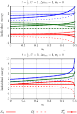
Figure 1: Unshifted $\mathcal{E}^{\mathbf{w}}_{K=0,1,2}$ and LZ-shifted $\overline{\mathcal{E}}^{\mathbf{w}}_{K=0,1,2}$ KS energies obtained for the asymmetric Hubbard dimer by varying the first ensemble weight while fixing the second one to zero. Results are shown for $U/t=2$ (top panel) and $U/t=10$ (bottom panel). Comparison is made with the exact energies $E_{K=0,1,2}$. First and second excited-state energies are shown in green and blue, respectively. EEXX-only results (including both LZ shift and ensemble xc derivative corrections) are also plotted in the top panel (with squares) for analysis purposes.

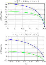
Figure 2: Exact ensemble xc derivatives obtained from Eqs. (6) and (14) for the asymmetric ($\Delta v_{\rm ext}/t=2$) Hubbard dimer with $U/t=2$. First- ($I=1$) and second-excited-state ($I=2$) derivatives are calculated for the true (weight-dependent) ensemble density generated from $\Delta v_{\rm ext}$ and are plotted (in green and blue, respectively) as functions of the first ensemble weight ${\tt w}_{1}$ for ${\tt w}_{2}=0$ (top panel) and ${\tt w}_{2}=1/4$ (bottom panel).

As illustrated in Fig. 1, the unshifted KS energies are found to be substantially lower than the exact energies. It is particularly striking for the first excited state whose unshifted KS energy equals zero, by construction (see Sec. III). In the symmetric case (see the Appendix B and the supplementary material), the ground- and second-excited-state unshifted KS energies are equal to $-2t$ and $2t$, respectively. As a result, varying the ensemble weights has no impact. The situation is different in the asymmetric case since the unshifted energies can vary with the weights through the density-functional KS potential. The second (doubly-) excited-state energy can for example be substantially improved when increasing the weights. However, the ground-state energy deteriorates in that case.

If we now apply the (weight-dependent) LZ shift, more accurate energies are obtained, as shown in Fig. 1. Note that, by construction, the LZ-shifted KS ground-state energy is exact when ${\tt w}_{1}={\tt w}_{2}=0$. It is important to notice that, unlike the exact energies, the LZ-shifted ones are (sometimes strongly) weight-dependent, thus illustrating the importance of modeling ensemble xc derivative corrections. The latter are plotted in Fig. 2. Interestingly, both first- and second-excited-state derivatives are non-negligible and will therefore contribute to the exact ground-state energy away from the $\mathbf{w}=0$ limit (see the second term on the right-hand side of Eq. (20)). Note also that these derivatives are strongly state-dependent. In the asymmetry and correlation regimes considered in Fig. 2, each derivative vanish for particular (state-dependent) weight values. In this case, the corresponding excitation energy is exactly equal to the KS one (see Eq. (14)).

Returning to the LZ-shifted KS energies, their weight dependence becomes even more important in stronger correlation regimes, as shown in the bottom panel of Fig. 1. Note that, in this case, the first and second excited states are single- and double-charge transfer states, respectively Deur et al. (2017). Note also that the first-weight-dependence of the shifted energies is sensitive to the value of the second weight, as shown in the supplementary material. Interestingly, increasing the ensemble weights can provide more accurate excited-state LZ-shifted energies, often at the expense of deteriorated ground-state energies. As shown in Fig. 1 (see also the supplementary material), this is a general trend that can be seen in all correlation regimes.

Finally, in order to assess the importance of correlation effects in the calculation of individual energy levels, we computed EEXX-only LZ shift and ensemble derivative corrections to the unshifted KS energies. Since we used exact densities (and therefore exact KS potentials), the LZ shift has been computed with the full (exact) Hxc potential in conjunction with the EEXX energy, for the sake of consistency. In the moderately correlated $U/t=2$ regime (see the top panel of Fig. 1), relatively good total energies are obtained, which is in agreement with the DEC/EEXX results of Ref. Sagredo and Burke (2018). Interestingly, the doubly-excited state energy is the one that exhibits the weakest weight dependence. As shown in Fig. 3, in the $\Delta v_{\rm ext}/t=2$ asymmetry regime, EEXX fails dramatically for the larger $U/t=10$ value. Total energies become strongly weight-dependent and their ordering is wrong for a wide range of weight values. The latter observation was actually expected for small weight values on the basis of Ref. Deur et al. (2017) (where we see in Fig. 1 that, for $2t=1$, $U=5$ and $\Delta v_{\rm ext}=1$, the ground-state density is close to 1, which corresponds to the symmetric case) and Appendix B, where the EEXX energies are derived for the symmetric Hubbard dimer (see Eq. (41)).

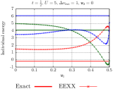
Figure 3: Ground- (red), first- (green) and second- (blue) excited-state energies (exact and EEXX-only) plotted as functions of the first ensemble weight (with ${\tt w}_{2}=0$) for the asymmetric ($\Delta v_{\rm ext}/t=2$) Hubbard dimer with $U/t=10$.

V Single versus sequence of ensemble calculations

While, in conventional GOK-DFT approaches, excitation (or individual) energies are extracted from a sequence of ensemble calculations (where ensemble weights are controlled by a single one $w$), we have shown in this work that a single ensemble calculation is sufficient provided, of course, that the many-weight-dependence of the ensemble xc functional is known. The two approaches are equivalent in the exact theory but they may give different results when density-functional approximations are used. This is analyzed further in the rest of this section at the EEXX level of approximation.

Let us first rewrite the exact individual energy expressions within the GOKII approach Yang et al. (2017) (see Eq. (3)) where both bi- and tri-ensemble calculations are needed for extracting the three lowest energies. From the bi-ensemble energy

$$E^{(w,0)}=(1-w)E_{0}+wE_{1},$$ (29)

we can extract both ground- and first-excited-state energies as follows,

$$E_{0} = E^{(w,0)}-w\dfrac{dE^{(w,0)}}{dw},$$

$$E_{1} = E^{(w,0)}+(1-w)\dfrac{dE^{(w,0)}}{dw},$$ (30)

which is equivalent (for these two states) to a tri-ensemble calculation where ${\tt w}_{1}=w$ and ${\tt w}_{2}=0$. On the other hand, we have the tri-ensemble energy (with ${\tt w}_{1}={\tt w}_{2}=w$),

$$E^{(w,w)}=(1-2w)E_{0}+wE_{1}+wE_{2},$$ (31)

from which we can extract, when combined with the bi-ensemble one, the second-excited-state energy:

$$E_{2} = E_{0}-(E_{1}-E_{0})+\dfrac{dE^{(w,w)}}{dw}$$ (32)

$$= E^{(w,0)}-(1+w)\dfrac{dE^{(w,0)}}{dw}+\dfrac{dE^{(w,w)}}{dw}.$$

If, like in Sec. III, we use a single ensemble calculation instead (with ${\tt w}_{1}={\tt w}_{2}=w$ for ease of comparison), then individual energies will be determined as follows (see Eq. (9)),

$$E_{0} = E^{(w,w)}-w\left.\dfrac{\partial E^{(w,{\tt w}_{2})}}{\partial w}\right|_{{\tt w}_{2}=w}-w\left.\dfrac{\partial E^{({\tt w}_{1},w)}}{\partial w}\right|_{{\tt w}_{1}=w}$$ (33)

$$= E^{(w,w)}-w\dfrac{dE^{(w,w)}}{dw},$$

and

$$E_{1} = E_{0}+\left.\dfrac{\partial E^{(w,{\tt w}_{2})}}{\partial w}\right|_{{\tt w}_{2}=w},$$

$$E_{2} = E_{0}+\left.\dfrac{\partial E^{({\tt w}_{1},w)}}{\partial w}\right|_{{\tt w}_{1}=w}.$$ (34)

Note that we use the latter expressions rather than the (equivalent) ones in Eq. (20) for ease of comparison.

As readily seen from Eqs. (V)-(33), the two approaches become identical (and equivalent to DEC Yang et al. (2017); Sagredo and Burke (2018)) in the $w\rightarrow 0$ limit, even when approximate ensemble energies are used. For larger $w$ values (in the range $0<w\leq 1/3$), the two methods will give substantially different results for the excited states when the EEXX-only approximation is used, as illustrated in Fig. 4. While, in our (single-calculation-based) approach, individual energies are increasingly insensitive to the value of the tri-ensemble weight as $U/t$ increases, the GOKII excited-state energies exhibit an important weight dependence. Interestingly, as $w$ increases, they become closer to the exact energies. In the large $U/t$ regime (see the bottom panel of Fig. 4), increasing $w$ restores the correct ordering of the excited states.

In the Hubbard dimer, the EEXX-only individual energies can be expressed as explicit functionals of the ensemble density (see Appendix C), thus allowing for a better understanding of these results. The key difference between GOKII and the single tri-ensemble calculation approach is the ensemble density itself. As $U/\Delta v_{\rm ext}$ and $\Delta v_{\rm ext}/t$ increase, the tri-ensemble density becomes closer to 1 (see Appendix C), thus explaining why tri-ensemble-based-only energies are essentially the (weight-independent) ones obtained at the symmetric EEXX level. Note that, in the latter case, the excited states are wrongly ordered (see Appendix B). On the other hand, the bi-ensemble density varies as $1+w$ in the same asymmetry and correlation regime. As a result, analytical expressions can be derived for the variation in $U$ and $w$ of the GOKII/EEXX energies (see Eqs. (C) and (C)), thus providing a rationale for the results shown in Fig. 4. As proven in Appendix C, the improvement of the second-excited-state energy as $w$ increases is exclusively due to the bi-ensemble contribution (two first terms on the right-hand side of Eq. (32)). The good performance of GOKII/EEXX (in terms of total excited-state energies) may be specific to the Hubbard dimer. Nevertheless, it clearly shows that the choice of ensemble and extraction procedure is crucial when using density-functional approximations.

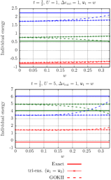
Figure 4: Comparison of single tri-ensemble (with ${\tt w}_{1}={\tt w}_{2}=w$) and GOKII approaches at the EEXX-only level of approximation in the asymmetric Hubbard dimer for $U/t=2$ (top panel) and $U/t=10$ (bottom panel). Red, green and blue colors are used for the ground, first and second excited states, respectively. See text for further details.

VI Conclusions and perspectives

A generalized many-weight-dependent formulation of GOK-DFT has been explored, thus leading to an in-principle-exact energy level extraction procedure that applies to any (ground or excited) state in the ensemble and relies on a single ensemble DFT calculation. The latter consists, like a conventional DFT calculation, in solving a single set of self-consistent KS equations where the orbitals are fractionally occupied (the occupation numbers are determined from the ensemble weights). The theory has been applied to the Hubbard dimer. The two corrections that should in principle be added to the bare KS energies (namely the global LZ shift and a state-specific (ensemble-based) xc derivative correction) were both shown to be important in the calculation of accurate and weight-independent energy levels. In order to turn the method into a practical computational tool, ab initio many-weight-dependent xc density-functional approximations should be developed. This can be achieved, for example, by applying GOK-DFT to finite uniform electron gases Loos (2017). A nice feature of such model systems is that both ground and excited states share the same density which is the ensemble density itself. Consequently, in this particular case, the density-functional ensemble xc energy is simply the weighted sum of the individual-state xc energies. Work is currently in progress in this direction. Finally, regarding the application of the theory to photochemical processes, we would like to explore the possibility of extracting non-adiabatic couplings from a GOK-DFT calculation. It may be useful, for that purpose, to extend the theory to the time-dependent linear response regime. This is left for future work.

VII Supplementary Material

We provide complementary curves showing the variation in the first ensemble weight ${\tt w}_{1}$ of individual energy levels (before and after the LZ shift) for ${\tt w}_{2}=0$ or ${\tt w}_{2}=1/4$ in various correlation and asymmetry regimes of the Hubbard dimer.

Appendix A Connection between exact tri- and bi-ensemble functionals

We start from the Lieb-maximization-based expression for the three-state ensemble analog of the ($U$- and $t$-dependent) Hohenberg–Kohn (HK) functional which reads in this context Deur et al. (2017),

$$F^{\mathbf{w}}(n)=\sup_{\Delta v}\Big{\{} \left(1-{\tt w}_{1}-{\tt w}_{2}\right)E_{0}(\Delta v)+{\tt w}_{1}E_{1}(\Delta v)$$ (35)

$$+{\tt w}_{2}E_{2}(\Delta v)-{\Delta v}(1-n)\Big{\}}.$$

Since the three singlet energies sum up to $2U$ (see Eq. (26) in Ref. Senjean et al. (2017)), the expression in Eq. (35) can be simplified as follows,

$$F^{\mathbf{w}}(n) = 2U{\tt w}_{2}+\sup_{\Delta v}\Big{\{}\left(1-{\tt w}_{1}-2{\tt w}_{2}\right)E_{0}(\Delta v)$$ (36)

$$+({\tt w}_{1}-{\tt w}_{2})E_{1}(\Delta v)-{\Delta v}(1-n)\Big{\}},$$

which can then be rewritten formally as

$$F^{\mathbf{w}}(n) = 2U{\tt w}_{2}+(1-3{\tt w}_{2})F^{w}(\nu),$$ (37)

where $w=({{\tt w}_{1}-{\tt w}_{2}})/({1-3{\tt w}_{2}})$ and $\nu=(n-3{\tt w}_{2})/(1-3{\tt w}_{2})$ are effective bi-ensemble weight and density, respectively, and the corresponding bi-ensemble functional reads Deur et al. (2017, 2018)

$$F^{w}(\nu)=\sup_{\Delta v}\{ (1-w)E_{0}(\Delta v)+{w}E_{1}(\Delta v)$$ (38)

$$-{\Delta v}(1-\nu)\}.$$

From the non-interacting ($U=0$) limit of Eq. (37) and Eq. (57) in Ref. Deur et al. (2017) we obtain the expression for the tri-ensemble non-interacting kinetic energy in Eq. (26). Since the Hx energy is the first-order contribution to the Taylor expansion in $U$ of the ensemble HK functional Gould and Pittalis (2017); Deur et al. (2018), it comes from Eq.(37),

$$E^{\mathbf{w}}_{\rm x}(n) = 2U{\tt w}_{2}+(1-3{\tt w}_{2})E_{\rm x}^{w}\left(\nu\right)$$ (39)

$$+(1-3{\tt w}_{2})E_{\rm H}\left(\nu\right)-E_{\rm H}(n),$$

thus leading, with Eq. (62) of Ref. Deur et al. (2017), to the expression in Eq. (27). The correlation energy corresponds to all higher-order contributions in $U$ to the HK functional, which leads to the scaling relation in Eq. (28).

Appendix B Symmetric Hubbard dimer

In the particular case of a symmetric dimer ($\Delta v_{\rm ext}=0$), the LZ-shifted KS energies can be simplified as follows, $\overline{\mathcal{E}}^{\mathbf{w}}_{0}=-2t+C^{\mathbf{w}}_{\rm LZ}$, $\overline{\mathcal{E}}^{\mathbf{w}}_{1}=C^{\mathbf{w}}_{\rm LZ}$, and $\overline{\mathcal{E}}^{\mathbf{w}}_{2}=2t+C^{\mathbf{w}}_{\rm LZ}$, where the shift equals

$$C^{\mathbf{w}}_{\rm LZ} = E^{\mathbf{w}}_{\rm Hxc}(n=1)=\dfrac{U}{2}(1+{\tt w}_{1})$$ (40)

$$+2t(1-2{\tt w}_{2}-{\tt w}_{1}).\left(1-\sqrt{1+[{U^{2}}/({16t^{2})]}}\right).$$

As readily seen from Eq. (40) [see also the plots in the supplementary material], these energies are weight-dependent, thus illustrating the importance of the ensemble xc derivative corrections in the calculation of physical (weight-independent) energies. Interestingly, if correlation is neglected in both the LZ shift and the ensemble derivative corrections [the approximation is referred to as EEXX in the text], we obtain the following weight-independent energy expressions,

$$E^{\rm EEXX}_{0}=-2t+\dfrac{U}{2},\hskip 2.84544ptE^{\rm EEXX}_{1}=U,\hskip 2.84544ptE^{\rm EEXX}_{2}=2t+\dfrac{U}{2}.$$ (41)

While EEXX (which can be seen as perturbation theory through first order in $U/t$) gives the exact energy level for the first (symmetric) excited state in all correlation regimes, the individual energy levels are well described for the ground and second excited states only in the symmetric weakly correlated regime (i.e. for small $U/t$ values). When the correlation is strong, the excited levels are actually wrongly ordered. Note that, in the symmetric case, the second (double) excitation energy is not affected by the EEXX-only derivative correction. Indeed, for $n=1$, the EEXX density functional does not vary with ${\tt w}_{2}$ (see Eq. (27)) and, therefore, the second-excited-state ensemble derivative is equal to zero. This result was expected on the basis of the recently published DEC/EEXX results for the Hubbard dimer (see Eq. (6) of Ref. Sagredo and Burke (2018)) and Eq. (22).

Appendix C Expressions for bi- and tri-ensemble-based EEXX density-functional energies

In order to derive analytical expressions for the energy levels within the EEXX approximation, we start from the general ensemble EEXX-only density-functional energy expression,

$$E^{\mathbf{w}}_{\rm EEXX}(n) = T_{\rm s}^{\mathbf{w}}(n)+E_{\rm H}(n)+E^{\mathbf{w}}_{\rm x}(n)$$ (42)

$$+(1-n)\Delta v_{\rm ext},$$

and the corresponding ensemble derivatives,

$$\dfrac{\partial E^{\mathbf{w}}_{\rm EEXX}(n)}{\partial{\tt w}_{1}}=\dfrac{2t(1-{\tt w}_{1}-2{\tt w}_{2})}{\sqrt{(1-{\tt w}_{1}-2{\tt w}_{2})^{2}-(1-n)^{2}}}$$

$$+\dfrac{U}{2}\left[1-\dfrac{\Big{(}1-3(2{\tt w}_{2}-{\tt w}_{1})\Big{)}(1-n)^{2}}{(1-{\tt w}_{1}-2{\tt w}_{2})^{3}}\right]$$ (43)

and

$$\dfrac{\partial E^{\mathbf{w}}_{\rm EEXX}(n)}{\partial{\tt w}_{2}}=\dfrac{4t(1-{\tt w}_{1}-2{\tt w}_{2})}{\sqrt{(1-{\tt w}_{1}-2{\tt w}_{2})^{2}-(1-n)^{2}}}$$

$$-\dfrac{2U(3{\tt w}_{1}-1)(1-n)^{2}}{(1-{\tt w}_{1}-2{\tt w}_{2})^{3}}.$$ (44)

The ensemble density-functional energies and derivatives from which we can extract individual energies within both GOKII and tri-ensemble-only approaches are

$$E_{\rm EEXX}^{(w,0)}(n)=-2t\sqrt{(1-{w})^{2}-(1-n)^{2}}$$

$$+\dfrac{U}{2}\left[1+{w}-\dfrac{(3{w}-1)(1-n)^{2}}{(1-{w})^{2}}\right]+(1-n)\Delta v_{\rm ext},$$ (45)

$$\dfrac{dE_{\rm EEXX}^{(w,0)}(n)}{dw}=\dfrac{2t(1-{w})}{\sqrt{(1-{w})^{2}-(1-n)^{2}}}$$

$$+\dfrac{U}{2}\left[1-\dfrac{(1+3{w})(1-n)^{2}}{(1-{w})^{3}}\right],$$ (46)

$$E_{\rm EEXX}^{(w,w)}(n)=-2t\sqrt{(1-3{w})^{2}-(1-n)^{2}}$$

$$+\dfrac{U}{2}\left[1+{w}-\dfrac{(1-n)^{2}}{(3w-1)}\right]+(1-n)\Delta v_{\rm ext},$$ (47)

$$\left.\dfrac{\partial E_{\rm EEXX}^{(w,{\tt w}_{2})}(n)}{\partial w}\right|_{{\tt w}_{2}=w} = \dfrac{2t(1-3{w})}{\sqrt{(1-3{w})^{2}-(1-n)^{2}}}$$ (48)

$$+\dfrac{U}{2}\left[1-\dfrac{(1-n)^{2}}{(1-3{w})^{2}}\right],$$

and

$$\left.\dfrac{\partial E_{\rm EEXX}^{({\tt w}_{1},w)}(n)}{\partial w}\right|_{{\tt w}_{1}=w} = \dfrac{4t(1-3{w})}{\sqrt{(1-3{w})^{2}-(1-n)^{2}}}$$ (49)

$$+2U\dfrac{(1-n)^{2}}{(1-3{w})^{2}}.$$

At the GOKII/EEXX level, the energies are approximated as follows,

$$E_{0} \approx E^{{\rm EEXX}}_{0}\left(n^{(w,0)}\right),$$

$$E_{1} \approx E^{{\rm EEXX}}_{1}\left(n^{(w,0)}\right),$$

$$E_{2} \approx E^{{\rm EEXX}(b)}_{2}\left(n^{(w,0)}\right)+E^{{\rm EEXX}(t)}_{2}\left(n^{(w,w)}\right),$$ (50)

where the (physical) bi- and tri-ensemble densities can be written as

$$n^{(w,0)}=(1-w)n^{0}_{\Delta v_{\rm ext}}+w\,n^{1}_{\Delta v_{\rm ext}}$$ (51)

and

$$n^{(w,w)} = (1-2w)n^{0}_{\Delta v_{\rm ext}}+w\,n^{1}_{\Delta v_{\rm ext}}+w\,n^{2}_{\Delta v_{\rm ext}}$$ (52)

$$= 3w+(1-3w)n^{0}_{\Delta v_{\rm ext}},$$

respectively. Note that, in Eq. (52), we used the fact that the three singlet densities (which are obtained by differentiating the energies with respect to the external potential Deur et al. (2017)) sum up to 3, as a consequence of the fact that the energies sum up to $2U$ (which does not depend on the external potential). The density-functional ground- and first-excited-state energies in Eq. (C) are

$$E^{{\rm EEXX}}_{0}\left(n\right) = E_{\rm EEXX}^{(w,0)}(n)-w\dfrac{dE_{\rm EEXX}^{(w,0)}(n)}{dw},$$

$$E^{{\rm EEXX}}_{1}\left(n\right) = E_{\rm EEXX}^{(w,0)}(n)+(1-w)\dfrac{dE_{\rm EEXX}^{(w,0)}(n)}{dw},$$ (53)

while the bi- and tri-ensemble contributions to the second-excited-state energy (see Eq. (32)) are

$$E^{{\rm EEXX}(b)}_{2}\left(n\right)=E_{\rm EEXX}^{(w,0)}(n)-(1+w)\dfrac{dE_{\rm EEXX}^{(w,0)}(n)}{dw},$$

and

$$E^{{\rm EEXX}(t)}_{2}\left(n\right) = \dfrac{6t(1-3{w})}{\sqrt{(1-3{w})^{2}-(1-n)^{2}}}$$ (55)

$$+\dfrac{U}{2}\left[1+3\dfrac{(1-n)^{2}}{(1-3{w})^{2}}\right],$$

respectively. Note that, in the symmetric case, the three energies obtained from Eq. (C) are $-2t+(U/2)$, $U$, and $2t+(U/2)$, which is exactly what is obtained when performing a single tri-ensemble calculation (see Appendix B).

In the particular case where $t<<\Delta v_{\rm ext}<<U$, we have $n^{0}_{\Delta v_{\rm ext}}\approx 1$ and $n^{1}_{\Delta v_{\rm ext}}\approx 2$ (see Fig. 1 in Ref.  Deur et al. (2017)). The bi- and tri-ensemble densities are then equal to $n^{(w,0)}=1+w$ and $n^{(w,w)}=1$, respectively. Consequently, the tri-ensemble contribution to the second-excited-state energy becomes weight-independent and equal to $6t+(U/2)$ while the bi-ensemble contribution varies in $w$ as follows,

$$\left.E^{{\rm EEXX}(b)}_{2}\left(n\right)\right|_{n=1+w}\approx\dfrac{Uw^{2}\left(1+3w^{2}\right)}{(1-w)^{3}}-w\Delta v_{\rm ext}.$$

We can show similarly that the ground- and first-excited-state energies vary in $w$ as follows,

$$\left.E^{{\rm EEXX}}_{0}\left(n\right)\right|_{n=1+w} \approx \dfrac{U}{2}+\dfrac{Uw^{2}[1+3w(2w-1)]}{2(1-w)^{3}}-w\Delta v_{\rm ext},$$

$$\left.E^{{\rm EEXX}}_{1}\left(n\right)\right|_{n=1+w} \approx U-\dfrac{3Uw^{3}}{(1-w)^{2}}-w\Delta v_{\rm ext}.$$ (57)

Turning to the single tri-ensemble calculation approach, individual energies can be approximated as follows at the EEXX level,

$$E_{K}\approx\mathcal{E}^{{\rm EEXX}}_{K}\left(n^{(w,w)}\right),$$ (58)

where, according to Eqs. (33) and (V),

$$\mathcal{E}^{{\rm EEXX}}_{0}\left(n\right)=E_{\rm EEXX}^{(w,w)}(n)$$

$$-w\left(\left.\dfrac{\partial E_{\rm EEXX}^{(w,{\tt w}_{2})}(n)}{\partial w}\right|_{{\tt w}_{2}=w}+\left.\dfrac{\partial E_{\rm EEXX}^{({\tt w}_{1},w)}(n)}{\partial w}\right|_{{\tt w}_{1}=w}\right),$$ (59)

$$\mathcal{E}^{{\rm EEXX}}_{1}\left(n\right)=\mathcal{E}^{{\rm EEXX}}_{0}\left(n\right)+\left.\dfrac{\partial E_{\rm EEXX}^{(w,{\tt w}_{2})}(n)}{\partial w}\right|_{{\tt w}_{2}=w},$$ (60)

and

$$\mathcal{E}^{{\rm EEXX}}_{2}\left(n\right)=\mathcal{E}^{{\rm EEXX}}_{0}\left(n\right)+\left.\dfrac{\partial E_{\rm EEXX}^{({\tt w}_{1},w)}(n)}{\partial w}\right|_{{\tt w}_{1}=w}.$$ (61)

References

- Runge and Gross (1984) E. Runge and E. K. Gross, Phys. Rev. Lett. 52, 997 (1984).
- Casida and Huix-Rotllant (2012) M. Casida and M. Huix-Rotllant, Annu. Rev. Phys. Chem. 63, 287 (2012).
- Gross et al. (1988a) E. K. U. Gross, L. N. Oliveira, and W. Kohn, Phys. Rev. A 37, 2809 (1988a).
- Oliveira et al. (1988) L. Oliveira, E. Gross, and W. Kohn, Phys. Rev. A 37, 2821 (1988).
- Gross et al. (1988b) E. K. U. Gross, L. N. Oliveira, and W. Kohn, Phys. Rev. A 37, 2805 (1988b).
- Theophilou (1979) A. K. Theophilou, J. Phys. C: Solid State Phys. 12, 5419 (1979).
- Theophilou (1987) A. K. Theophilou, The single particle density in physics and chemistry, edited by N. H. March and B. M. Deb (Academic Press, 1987) pp. 210–212.
- Helgaker et al. (2004) T. Helgaker, P. Jørgensen, and J. Olsen, “Molecular electronic-structure theory,” (Wiley, Chichester, 2004) pp. 598–647.
- Nagy (1995) A. Nagy, Int. J. Quantum Chem. 56, 225 (1995).
- Gidopoulos et al. (2002) N. I. Gidopoulos, P. G. Papaconstantinou, and E. K. U. Gross, Phys. Rev. Lett. 88, 033003 (2002).
- Pastorczak et al. (2013) E. Pastorczak, N. I. Gidopoulos, and K. Pernal, Phys. Rev. A 87, 062501 (2013).
- Franck and Fromager (2014) O. Franck and E. Fromager, Mol. Phys. 112, 1684 (2014).
- Yang et al. (2014) Z.-h. Yang, J. R. Trail, A. Pribram-Jones, K. Burke, R. J. Needs, and C. A. Ullrich, Phys. Rev. A 90, 042501 (2014).
- Pribram-Jones et al. (2014) A. Pribram-Jones, Z. hui Yang, J. R.Trail, K. Burke, R. J.Needs, and C. A.Ullrich, J. Chem. Phys. 140, 18A541 (2014).
- Pernal et al. (2016) K. Pernal, N. I. Gidopoulos, and E. Pastorczak, in Adv. Quantum Chem., Vol. 73 (Elsevier, 2016) pp. 199–229.
- Yang et al. (2017) Z.-h. Yang, A. Pribram-Jones, K. Burke, and C. A. Ullrich, Phys. Rev. Lett. 119, 033003 (2017).
- Gould and Pittalis (2017) T. Gould and S. Pittalis, Phys. Rev. Lett. 119, 243001 (2017).
- Gould et al. (2018) T. Gould, L. Kronik, and S. Pittalis, J. Chem. Phys. 148, 174101 (2018).
- Deur et al. (2017) K. Deur, L. Mazouin, and E. Fromager, Phys. Rev. B 95, 035120 (2017).
- Deur et al. (2018) K. Deur, L. Mazouin, B. Senjean, and E. Fromager, Eur. Phys. J. B 91, 162 (2018).
- Gould and Pittalis (2018) T. Gould and S. Pittalis, arXiv:1808.04994 (2018).
- Sagredo and Burke (2018) F. Sagredo and K. Burke, J. Chem. Phys. 149, 134103 (2018).
- Senjean and Fromager (2018) B. Senjean and E. Fromager, Phys. Rev. A 98, 022513 (2018).
- Nikiforov et al. (2014) A. Nikiforov, J. A. Gamez, W. Thiel, M. Huix-Rotllant, and M. Filatov, J. Chem. Phys. 141, 124122 (2014).
- Filatov (2015) M. Filatov, WIREs Comput. Mol. Sci. 5, 146 (2015).
- Filatov et al. (2015) M. Filatov, M. Huix-Rotllant, and I. Burghardt, J. Chem. Phys. 142, 184104 (2015).
- Filatov et al. (2016) M. Filatov, F. Liu, K. S. Kim, and T. J. Martínez, J. Chem. Phys. 145, 244104 (2016).
- Filatov et al. (2017) M. Filatov, T. J. Martínez, and K. S. Kim, J. Chem. Phys. 147, 064104 (2017).
- Senjean et al. (2015) B. Senjean, S. Knecht, H. J. Aa. Jensen, and E. Fromager, Phys. Rev. A 92, 012518 (2015).
- Ayers et al. (2012) P. W. Ayers, M. Levy, and A. Nagy, Phys. Rev. A 85, 042518 (2012).
- Ayers et al. (2015) P. W. Ayers, M. Levy, and A. Nagy, J. Chem. Phys. 143, 191101 (2015).
- Ayers et al. (2018) P. W. Ayers, M. Levy, and Á. Nagy, Theor. Chem. Acc. 137, 152 (2018).
- Levy and Zahariev (2014) M. Levy and F. Zahariev, Phys. Rev. Lett. 113, 113002 (2014).
- Levy (1995) M. Levy, Phys. Rev. A 52, R4313 (1995).
- Carrascal et al. (2015) D. J. Carrascal, J. Ferrer, J. C. Smith, and K. Burke, J. Phys. Condens. Matter 27, 393001 (2015).
- Carrascal et al. (2016) D. Carrascal, J. Ferrer, J. Smith, and K. Burke, J. Phys. Condens. Matter 29, 019501 (2016).
- Li et al. (2018) C. Li, R. Requist, and E. K. U. Gross, J. Chem. Phys. 148, 084110 (2018).
- Carrascal et al. (2018) D. J. Carrascal, J. Ferrer, N. Maitra, and K. Burke, Eur. Phys. J. B 91, 142 (2018).
- Ullrich (2018) C. A. Ullrich, Phys. Rev. B 98, 035140 (2018).
- Loos (2017) P.-F. Loos, J. Chem. Phys. 146, 114108 (2017).
- Senjean et al. (2017) B. Senjean, M. Tsuchiizu, V. Robert, and E. Fromager, Mol. Phys. 115, 48 (2017).