A MOM-based ensemble method for robustness, subsampling and hyperparameter tuning

Abstract

Hyperparameters tuning and model selection are important steps in machine learning. Unfortunately, classical hyperparameter calibration and model selection procedures are sensitive to outliers and heavy-tailed data. In this work, we construct a selection procedure which can be seen as a robust alternative to cross-validation and is based on a median-of-means principle [1, 24, 41]. Using this procedure, we also build an ensemble method which, trained with algorithms and corrupted heavy-tailed data, selects an algorithm, trains it with a large uncorrupted subsample and automatically tune its hyperparameters. The construction relies on a divide-and-conquer methodology [25], making this method easily scalable for autoML given a corrupted database. This method is tested with the LASSO [49] which is known to be highly sensitive to outliers.

1 Introduction

Robustness has become an important subject of interest in the machine learning community over the last few years because large datasets are very likely to be corrupted. This may happen due to hardware, storage or transmission issues, for instance, or as a result of (human) reporting errors. As can be seen, for instance, in Figure 1 in [29] and Figure 1 and 5 in [30], many learning algorithms based on emprical risk minimization (including the LASSO) may be completely mislead by a single corrupted example.

Robust alternatives to empirical risk minimizers and their penalized/regularized versions have been studied in density estimation [5] and least-squares regression [4, 36, 20, 48, 53]. Various robust descent algorithms have also been recently considered [44, 42, 43, 23, 22]. Despite these important progresses, the final steps of a data-scientist routine, which are estimator selection and hyperparameter tuning [8, 11, 7] are yet to receive a proper treatment. In fact, practitioners usually have at disposal several algorithms, each of these requiring one or several parameters to be tuned. An alternative to estimator selection is aggregation (aka ensemble methods) [16, 51, 40] which outputs e.g. a linear or convex combination of the candidate estimators; classical examples include binning, boosting, bagging or stacking.

The most common procedure used to select or aggregate candidate estimators is (cross-)validation: the dataset is partitioned (several times in the case of cross-validation) into a training sample used to build candidate estimators and a test sample used to estimate their risks. The final estimator is either the candidate with lowest estimated risk, or a linear combination of the candidates with coefficients depending on the estimated risks. Even if some candidate estimators are robust, outliers from the test set may mislead the selection/aggregation step, resulting in a poor final estimator. This raises the question of a robust selection/aggregation procedure, which is addressed in the present work.

There exist many data-driven methods to tune hyperparameters or to select an estimator from a collection of candidates. Among these, one can mention the SURE method [47], model selection [8, 11, 12, 35, 9, 38] where penalization methods are used to select among candidates built with the same data as those used to build the original estimators, selection, convex or linear aggregation [51, 45, 52], cross-validation [2, 3] or Lepski [33] and the Goldenschluger-Lepski [21] methods to name a few. To the best of our knowledge, all these techniques either use a classical non-robust validation principle or estimate the risk with the non-robust empirical risk. A notable exception is the estimator selection procedure of [6, 7] which is robust in general settings [6] and extremely efficient in Gaussian linear regression [7]. The main drawback is that this procedure requires robust tests in Hellinger distance that may be hard to compute for general learning problems where one does not specify statistical models with bounded complexities.

The first contribution of this paper is a general and robust estimator selection procedure with provable theoretical guarantees, which can be viewed as a robust alternative to cross-validation. Roughly stated, the procedure uses a median-of-means principle [1, 24, 41] to build robust pairwise comparisons between candidates, and the final estimator is then selected by a minmax procedure in the spirit of [4, 28] or the Goldenshluger-Lepski method [21], see Section 3 for details. The method is easily implementable. We here focus on least-squares regression and refer to [34] for other examples including density estimation and classification.

The second contribution is the definition of an ensemble method based on this selection procedure and a subsampling strategy. Two of the main ideas behind this method is that subsampling can provide robustness by avoiding outliers and that the choice of the subsample can itself be seen an a hyperparameter to be tuned. Estimator selection procedures can then be used to simultaneously select the best algorithm, an uncorrupted subsample and the best hyperparameters. Moreover, the method is computationally attractive.

Subsampling is usually used in machine learning for computational reasons: some algorithms require to break large datasets into smaller pieces [25], for instance in supervised learning [17, for classification and regression] and [37, for matrix factorization]. A natural way to divide-and-conquer corresponds to the older idea of subagging [15, subsample aggregating]—which is a variant of bagging [14]: one randomly chooses several small subsets of data, build an estimator from each subsample, and aggregate them into a single estimator. For instance, the bag of little bootstraps [26] builds confidence intervals in such a way. Subagging is also used for large-scale sparse regression [13].

The paper is divided as follows. Section 2 presents the general prediction setting we consider, and Section 3 introduces the robust estimator selection procedure. Theoretical guarantees for the latter are given in Theorem 3.2. The ensemble method is defined in Section 4 and applied to the LASSO in Section 5. Applications to the ERM in linear aggregation are presented in Appendix A. Numerical experiments are presented in Section 6. The proofs are outsourced in the appendix in Appendices B and C.

2 Setting

For positive integers $k\leqslant l$, let $[k]=\left\{1,2,\dots,k\right\}$, $\left\llbracket k,l\right\rrbracket=\left\{k,k+1,\dots,l\right\}$, and reversed double-bar brackets mean exclusion of the corresponding integer, e.g. $\left\rrbracket k,l\right\rrbracket=\left\{k+1,k+2,\dots,l\right\}$. We call partition of a set $E$ any family of disjoint subsets of $E$ with union equal to $E$.

Let $\mathbb{X}$ be a measurable space. Let $P$ be a probability distribution on $\mathbb{X}\times\mathbb{R}$, and let $(X,Y)\sim P$. Denote $P_{X}$ the marginal distribution of $X$. Assume that $\mathbb{E}\left[Y^{2}\right]<+\infty$. Denote $L^{2}(P_{X})$ the Hilbert space of measurable functions $f:\mathbb{X}\to\mathbb{R}$ such that $\mathbb{E}\left[f(X)^{2}\right]<+\infty$, the norm being denoted by $\left\|f\right\|=\sqrt{\mathbb{E}\left[f(X)^{2}\right]}$. For any probability measure $Q$ on $\mathbb{X}\times\mathbb{R}$ and any measurable function $g:\mathbb{X}\times\mathbb{R}\to\mathbb{R}$, that belongs to $L^{1}(Q)$, let $Q\left[g\right]:=\mathbb{E}_{Z\sim Q}\left[g(Z)\right]$.

Let $F$ be a linear subspace of $L^{2}(P_{X})$. We call estimator any element of $F$. For $f\in F$, let $\gamma(f):\mathbb{X}\times\mathbb{R}\to\mathbb{R}$ denote the square-loss function associated with $f$, defined by for all $(x,y)\in\mathbb{X}\times\mathbb{R}$ by $\gamma(f)(x,y)=(y-f(x))^{2}$. For any function $f:\mathbb{X}\to\mathbb{R}$ in $L^{2}(P_{X})$, let $R(f)$ denote its risk $R(f):=P\left[\gamma(f)\right]$ and let $f^{*}$ be the oracle: $f^{*}:=\operatorname*{arg\,min}_{f\in F}R(f)$. Let $\ell$ denote the excess risk with respect to $f^{*}$:

$$\ell(f)=R(f)-R(f^{*})=P\left[(f-f^{*})^{2}\right]=\left\|f-f^{*}\right\|^{2}.$$

The second equality holds since $F$ is a linear space. A learning algorithm is a measurable map $G\colon\bigcup_{n=1}^{+\infty}(\mathbb{X}\times\mathbb{R})^{n}\to F$ which takes a dataset of any (finite) size as input and outputs an estimator in $F$.

Assumption 1.

Let $\chi,\sigma>0$ such that for every $f\in F$,

$$(Pf^{4})^{1/4}\leqslant\chi(Pf^{2})^{1/2}\quad\text{and}\quad P\left[(Y-f^{*})^{2}(f-f^{*})^{2}\right]\leqslant\sigma^{2}P(f-f^{*})^{2}.$$

This assumption only involves second and fourth moments. The first assumption $(Pf^{4})^{1/4}\leqslant\chi(Pf^{2})^{1/2}$ is satisfied for instance by linear functions $f(\cdot)=\bigl{<}\cdot,t\bigr{>}$ for $t\in{\mathbb{R}}^{d}$ and $X$ which is a $d$-dimensional vectors with independent entries with a fourth moment [39]. It therefore covers heavy-tailed cases beyond classical $L_{\infty}$-boundedness or subgaussian assumptions. The second assumption $P\left[(Y-f^{*})^{2}(f-f^{*})^{2}\right]\leqslant\sigma^{2}P(f-f^{*})^{2}$ holds for instance when the noise $Y-f^{*}(X)$ is independent of $X$ and has a second moment—which is a very standard statistical modeling assumption when $Y=f^{*}(X)+\zeta$ with $\zeta$ independent of $X$. It also also holds when $Y-f^{*}(X)$ has a fourth moment by using Cauchy-Schwarz.

Let $N\geqslant 1$ be the size of the dataset $(X_{i},Y_{i})_{i\in[N]}$, which is partitioned into informative data and outliers: $[N]=\mathcal{O}\sqcup\mathcal{I}$. Informative data $(X_{i},Y_{i})_{i\in\mathcal{I}}$ is assumed independent and identically distributed (i.i.d.), with common distribution $P$. No assumption is granted on outliers $(X_{i},Y_{i})_{i\in\mathcal{O}}$. Of course, the partition $\mathcal{O}\sqcup\mathcal{I}$ is unknown to the learner. We call a subsample any nonempty subset $B\subset[N]$ (or the corresponding data $(X_{i},Y_{i})_{i\in B}$), and for any measurable function $g:\mathbb{X}\times\mathbb{R}\to\mathbb{R}$, denote:

$$P_{B}\left[g\right]=\frac{1}{\left|B\right|}\sum_{i\in B}g(X_{i},Y_{i}).$$

3 Minmax-MOM selection: a robust alternative to cross-validation

Let $(\hat{f}_{m})_{m\in\mathcal{M}}$ be a finite collection of estimators. For each index $m\in\mathcal{M}$, we assume that there exists a learning algorithm $G_{m}$ and a subsample $B_{m}\subset[N]$ of cardinality less than $N/4$ such that $\hat{f}_{m}$ is the estimator trained by algorithm $G_{m}$ using subsample $B_{m}$; in other words $\hat{f}_{m}=G_{m}((X_{i},Y_{i})_{i\in B_{m}})$ (the remaining of the dataset will be used to estimate the risk of the estimator, like in cross-validation). The best choice of $m\in{\cal M}$ regarding our final objective satisfies

$$\begin{split}m_{o}&:=\operatorname*{arg\,min}_{m\in{\cal M}}P\left[\gamma(\hat{f}_{m})\right]=\operatorname*{arg\,min}_{m\in{\cal M}}\max_{m^{\prime}\in{\cal M}}P\left[\gamma(\hat{f}_{m})-\gamma(\hat{f}_{m^{\prime}})\right]\enspace.\end{split}$$ (1)

However, the real-valued expectations $P\big{[}\gamma(\hat{f}_{m})-\gamma(\hat{f}_{m^{\prime}})\big{]}$ are unknown: let us construct a robust estimator of those quantities. Let $V\in\left\llbracket 1,N/8\right\rrbracket$. For each couple $(m,m^{\prime})\in\mathcal{M}^{2}$, let $(T_{v}^{(m,m^{\prime})})_{v\in[V]}$ be a partition into $V$ blocks of a subset of $[N]\setminus(B_{m}\cup B_{m^{\prime}})$, such that $\big{|}T_{v}^{(m,m^{\prime})}\big{|}\geqslant N/4V$ for all $v\in[V]$. The estimates $\mathcal{T}(m,m^{\prime})$ of $P\big{[}\gamma(\hat{f}_{m})-\gamma(\hat{f}_{m^{\prime}})\big{]}$ are defined by:

$$\mathcal{T}(m,m^{\prime}):=\operatorname*{med}_{v\in[V]}\left\{P_{T_{v}^{(m,m^{\prime})}}\left[\gamma(\hat{f}_{m})-\gamma(\hat{f}_{m^{\prime}})\right]\right\},$$

in other words, $\mathcal{T}(m,m^{\prime})$ is the median of the $V$ empirical means $P_{T_{v}^{(m,m^{\prime})}}\big{[}\gamma(\hat{f}_{m})-\gamma(\hat{f}_{m^{\prime}})\big{]},v\in[V]$. The selection of the final estimator is obtained by plugging these median-of-means (MOM) estimators into equation (1). In other words, we select $\hat{f}_{\widehat{m}}$, where

$$\hat{m}:=\operatorname*{arg\,min}_{m\in\mathcal{M}}\max_{m^{\prime}\in\mathcal{M}}\mathcal{T}(m,m^{\prime}).$$ (2)

Thanks to the median-of-mean operator, the risk of the selected estimator $\hat{f}_{\hat{m}}$ is expected to be close to the risk of the best estimator $\hat{f}_{m_{o}}$, even for heavy-tailed and corrupted data because $\mathcal{T}(m,m^{\prime})$ is a robust (to outliers) sub-gaussian estimator of $\gamma(\hat{f}_{m})-\gamma(\hat{f}_{m^{\prime}})$, even for heavy-tailed data [34].

Median-of-means have been introduced in [1, 24, 41]. Median-of-means pairwise comparisons have been used to build robust estimators in [36, 27]. Minmax strategies have been used in [4, 28] for least-squares regression and in [5] for density estimation. Finally, the minmax principle has been used for (non-robust) selection of estimators in [21].

Remark 3.1 (Minmax-MOM selection to divide-and-conquer).

It is classical to use divide-and-conquer approaches [25] to deal with large databases: the database is divided in small batches, algorithms are run on each batch and the results are “aggregated”. Minmax-MOM selection procedure (2) can perform this king of aggregation. Denote by $B_{m}$ the block of data hosted on server $m\in\mathcal{M}$. Train estimators $\hat{f}_{m}$ for all $m\in{\cal M}$. Then, for all $m,m^{\prime}\in{\cal M}$, compute the $V$ real numbers $P_{T_{v}^{(m,m^{\prime})}}\big{[}\gamma(\hat{f}_{m})-\gamma(\hat{f}_{m^{\prime}})\big{]},\ v\in[V]$ and take their median. Then compute the minmax-MOM estimator (if there are too many medians, choose $m$ and $m^{\prime}$ at random in $\mathcal{M}$). Following the map-reduce terminology [18], the mapper is the training of the procedure itself and the $V$ evaluations. The reducer is the computation of the $\binom{\left|\mathcal{M}\right|}{2}$ medians of differences of empirical risks and the minmax-MOM selection (2).

Theorem 3.2 (Robust oracle inequality).

Grant Assumption 1 and assume $V\in\left\llbracket 3\left|\mathcal{O}\right|,N/8\right\rrbracket$. Then with probability larger than $1-\left|\mathcal{M}\right|^{2}e^{-V/48}$, the estimator $\hat{f}_{\widehat{m}}$, where $\hat{m}$ is selected by the minmax-MOM selection procedure (2) satisfies, for all $\varepsilon>0$,

$$(1-a_{\varepsilon,V})\,\ell(\hat{f}_{\widehat{m}})\leqslant(1+3a_{\varepsilon,V})\,\min_{m\in\mathcal{M}}\ell(\hat{f}_{m})+2b_{\varepsilon,V},$$

where $f\mapsto\ell(f)=R(f)-R(f^{*})$ is the excess loss function, $a_{\varepsilon,V}:=8\chi^{2}\sqrt{2V/N}+2\sqrt{2}\varepsilon$ and $b_{\varepsilon,V}:=(64V\sigma^{2})/N\varepsilon$.

The proof of Theorem 3.2 is postponed to Section C.1. Roughly speaking, Theorem 3.2 states that, with exponentially large probability, the selected estimator (2) has the excess risk of the best estimator in the collection $(\hat{f}_{m})_{m\in\mathcal{M}}$. Following [19], this result is called an oracle inequality. We call it robust as it holds under moment assumptions on the linear space $F$ (see Assumption 1) and for a dataset that may contain outliers. The residual term $b_{\varepsilon,V}$ is of order $V/N$. If $\log|{\cal M}|\gtrsim|{\cal O}|$ and $V\asymp\log|{\cal M}|$, the residual term is of order $\log|{\cal M}|/N$, which is minimax optimal [50]. The oracle inequality is interesting when $a_{\varepsilon,V}<1$ which holds if $\chi\lesssim\sqrt{N/V}$. The “constant” $\chi$ in Assumption 1 may therefore grow with the dimension of $F$ as in the examples of [46] without breaking the results.

4 An ensemble method to induce robustness, subsampling and hyperparameters tuning

In this section, we define an ensemble method which takes one or several (non necessarily robust) algorithms as input and ouputs an estimator. The method is robust to the presence of outliers, has subsampling capabilities, and automatically tune hyperparameters. The main ideas behind the construction are: using subsampling as a way of achieving robustness (by avoiding outliers), viewing the choice of the subsample as a hyperparameter to be tuned, and using the robust selection procedure from Section 3 to select the final estimator. Performance guaranties are established in Corollary 4.1.

4.1 Definition of the method

Let $(G_{\lambda})_{\lambda\in\Lambda}$ be a finite collection of learning algorithms which outputs estimators in $F$. The collection may in fact correspond to a single algorithm with several combinations of hyperparameters values, or even several different algorithms with several combinations of hyperparameters values.

We now construct the set $\mathcal{B}$ of subsamples to be considered by the method. Assume $N\geqslant 8$. Let $K_{\text{min}}$ and $K_{\text{max}}$ integers such that $3\leqslant K_{\text{min}}\leqslant K_{\text{max}}\leqslant\log_{2}N$ (these parameters will specify the subsamples cardinality range). For each $K\in\left\llbracket K_{\text{min}},\ K_{\text{max}}\right\rrbracket$, consider a partition $(B_{k}^{(K)})_{k\in[2^{K}]}$ of $[N]$ such that for all $k\in[2^{K}]$, $\left\lfloor N/2^{K}\right\rfloor\leqslant\left|B_{k}^{(K)}\right|$. We call $(B_{k}^{(K)})_{k\in[2^{K}]}$ the $2^{K}$-partition. Let

$$\mathcal{B}=\bigcup_{K=K_{\text{min}}}^{K_{\text{max}}}\bigcup_{k\in[2^{K}]}\left\{B_{k}^{(K)}\right\}\quad\text{and}\quad{\cal M}=\Lambda\times\mathcal{B}.$$ (3)

From $K_{\text{min}}\geqslant 3$ we can easily deduce that each subsample in ${\cal B}$ has cardinality less than $N/4$. Then, as in Section 3, for each $m=(\lambda,B)$, let $\hat{f}_{m}$ be the estimator trained by algorithm $G_{\lambda}$ using subsample $B$, in other words: $\hat{f}_{m}=G_{\lambda}((X_{i},Y_{i})_{i\in B})$. Let $V\in\left\llbracket 3,N/8\right\rrbracket$. For each couple $(m,m^{\prime})\in\mathcal{M}^{2}$, let $(T_{v}^{(m,m^{\prime})})_{v\in[V]}$ be a partition of a subset of $[N]\setminus(B_{m}\cup B_{m^{\prime}})$ such that $\left|T_{v}^{(m,m^{\prime})}\right|\geqslant N/4V$ for all $v\in[V]$. Then, using the minmax-MOM selection procedure (2) from Section 3, we select from collection $(\hat{f}_{m})_{m\in{\cal M}}$ the final estimator $\hat{f}_{\hat{m}}$.

4.2 Theoretical guarantees

The following result states that if risk bounds hold for algorithms $(G_{\lambda})_{\lambda\in\Lambda}$ in a context with no-outlier, then $\hat{f}_{\widehat{m}}$ essentially satisfies the best of those risk bounds, even in the presence of outliers.

Corollary 4.1.

Let ${\cal M}$ be defined by (3). Grant Assumption 1. Let $\rho:\Lambda\times\mathbb{N}^{*}\to\mathbb{R}_{+}\cup\left\{+\infty\right\}$ be a non-increasing function in its second variable and $\nu:\Lambda\to\mathbb{R}_{+}^{*}$. Denote $\nu_{\text{max}}:=\lceil\max_{\lambda\in\Lambda}\nu(\lambda)\rceil$. Assume that $N\geqslant\nu_{\text{max}}\max(8V,2^{K_{\text{min}}+1})$ and $V\in\left\llbracket 3\left|\mathcal{O}\right|,2^{K_{\text{max}}-1}\right\rrbracket$. Assume that, for all $\lambda\in\Lambda$ and $B\subset\mathcal{I}$ such that $\left|B\right|\geqslant\nu(\lambda)$, it holds that $\ell(\hat{f}_{\lambda,B})\leqslant\rho(\lambda,\left|B\right|)$ with probability larger than $1-\exp(-1/48)$. Then for all $\varepsilon>0$, the estimator $\hat{f}_{\widehat{m}}$ defined in (2) satisfies

$$(1-a_{\varepsilon,V})\ell(\hat{f}_{\widehat{m}})\leqslant(1+3a_{\varepsilon,V})\,\min_{\lambda\in\Lambda}\rho\left(\lambda,\left\lfloor\frac{N}{\max(4V,2^{K_{\text{min}}})}\right\rfloor\right)+2b_{\varepsilon,V}$$ (4)

with probability larger than

$$1-(\left|\Lambda\right|^{2}N^{2}+1)e^{-V/48}.$$ (5)

Corollary 4.1 is proved in Section C.2. Let us stress some important aspects.

Estimators $\hat{f}_{\lambda,B}$ for $(\lambda,B)\in{\cal M}$ are assumed to satisfy an excess risk bound with rates $\rho(\lambda,\left|B\right|)$ only with constant probability (the constant $1-\exp(-1/48)$ chosen here has nothing special), when $B$ is large enough and only contains informative data. For example, this condition is met by ERM when informative data satisfies moment assumptions, see Propositions 5.2 and A.1. With these arguably weak requirement, the above statement claims that the ensemble method achieves the best bound among $\rho(\lambda,\left\lfloor N/\max(4V,2^{K_{\text{min}}})\right\rfloor),\ \lambda\in\Lambda$ with exponentially large probability (5).

The upper bound $\rho(\lambda,\left|B\right|)$ on the excess risk of $\hat{f}_{\lambda,B}$ depends on $\lambda$ and the size $\left|B\right|$ of the subsample. It improves with the sample size by the monotonicity assumption on $\rho$.

Finally, the function $\lambda\mapsto\nu(\lambda)$ is introduced to handle situations where the risk bound holds only when the sample size is larger than $\nu(\lambda)$.

4.3 An efficient partition scheme of the dataset

The partitions $(B_{k}^{(K)})_{k\in\left[2^{K}\right]}$ ($K\in\left\llbracket K_{\text{min}},\ K_{\text{max}}\right\rrbracket$) and $(T_{v}^{(m,m^{\prime})})_{v\in[V]}$ (for $(m,m^{\prime})\in\mathcal{M}^{2}$) can be constructed in many different ways. This section presents a specific choice for those partitions which yields a computational advantage by significantly reducing the number of empirical risks $P_{T_{v}^{(m,m^{\prime})}}[\gamma(\hat{f}_{m})]$ to be computed (by making many of them redundant). This complexity reduction makes the computations from Section 6 possible in a reasonable amount of time.

The minimax-MOM selection procedure (2) requires, for all $(m,m^{\prime})\in\mathcal{M}^{2}$ and $v\in[V]$, the computation of $P_{T_{v}^{(m,m^{\prime})}}\big{[}\gamma(\hat{f}_{m})\big{]}$ and $P_{T_{v}^{(m,m^{\prime})}}\big{[}\gamma(\hat{f}_{m^{\prime}})\big{]}$. Since the partition $(T_{v}^{(m,m^{\prime})})_{v\in[V]}$ may be different for each couple $(m,m^{\prime})\in\mathcal{M}^{2}$, this requires, in the worst case, the computation of $V\left|\mathcal{M}\right|^{2}$ empirical risks. By comparison, the construction presented here will only require the computation of $8V|{\cal M}|/3$ empirical risks.

For $K\in\left\llbracket 3,\ \lfloor\log_{2}N\rfloor\right\rrbracket$ and $k\in[2^{K}]$, define $B_{k}^{(K)}:=\left\rrbracket\left\lfloor\frac{(k-1)N}{2^{K}}\right\rfloor,\ \left\lfloor\frac{kN}{2^{K}}\right\rfloor\right\rrbracket$. For each $K\in\left\llbracket 3,\ \lfloor\log_{2}N\rfloor\right\rrbracket$, $(B_{k}^{(K)})_{k\in[2^{K}]}$ is a partition of $[N]$ such that, for each $k\in[2^{K}]$, $\lfloor N/2^{K}\rfloor\leqslant\big{|}B_{k}^{(K)}\big{|}\leqslant N/4$, as required. Moreover, the following key property holds.

Lemma 4.2.

Let $3\leqslant K^{\prime}\leqslant K\leqslant\lfloor\log_{2}N\rfloor$.

1. For all $k\in[2^{K}]$, $B_{k}^{(K)}\subset B^{(K^{\prime})}_{\lfloor(k-1)2^{K^{\prime}-K}\rfloor+1}$.

2. For all $k^{\prime}\in[2^{K^{\prime}}]$, $(B_{k}^{(K)})_{k\in\left\rrbracket(k^{\prime}-1)2^{K-K^{\prime}},\ k^{\prime}2^{K-K^{\prime}}\right\rrbracket}$ is a partition of $B_{k^{\prime}}^{(K^{\prime})}$.

Let

$$K_{0}:=\lceil\log_{2}(V/3)\rceil+2.$$ (6)

For all $K_{1},K_{2}\in\left\llbracket 3,\ \lfloor\log_{2}N\rfloor\right\rrbracket$ and $k_{1}\in\left[2^{K_{1}}\right]$, $k_{2}\in\left[2^{K_{2}}\right]$, let $\mathcal{K}_{0}(K_{1},k_{2},K_{2},k_{2})$ be the set of indices from the $2^{K_{0}}$-partition which have empty intersection with both $B_{k_{1}}^{(K_{1})}$ and $B_{k_{1}}^{(K_{2})}$:

$$\mathcal{K}_{0}(K_{1},k_{1},K_{2},k_{2}):=\left\{k\in\left[2^{K_{0}}\right]\,\middle|\,B_{k}^{(K_{0})}\cap(B_{k_{1}}^{(K_{1})}\cup B_{k_{2}}^{(K_{2})})=\varnothing\right\}.$$

Lemma 4.3.

For all $3\leqslant K_{1},K_{2}\leqslant\lfloor\log_{2}N\rfloor$ and $k_{1}\in\left[2^{K_{1}}\right]$, $k_{2}\in\left[2^{K_{2}}\right]$, we have $\left|\mathcal{K}_{0}(K_{1},k_{1},K_{2},k_{2})\right|\geqslant V$.

Let $(m,m^{\prime})\in\mathcal{M}^{2}$ and $K_{1},k_{1},K_{2},k_{2}$ be such that $B_{m}=B_{k_{1}}^{(K_{1})}\quad\text{and}\quad B_{m^{\prime}}=B_{k_{2}}^{(K_{2})}$. Then, the collection of sets $(B_{k}^{(K_{0})})_{k\in\mathcal{K}_{0}(K_{1},k_{1},K_{2},k_{2})}$ is a sub-collection of the $2^{K_{0}}$-partition, whose sets have empty intersection with both $B_{m}$ and $B_{m^{\prime}}$, and which, according to Lemma 4.3, contains at least $V$ sets. We can thus define $(T_{v}^{(m,m^{\prime})})_{v\in[V]}$ as a sub-collection of size exactly $V$. Consequently, $(T_{v}^{(m,m^{\prime})})_{v\in[V]}$ is indeed a partition of a subset of $[N]\setminus(B_{m}\cup B_{m^{\prime}})$. Moreover, we have the following lower bound on the cardinality of its sets, which is required (see Section 3).

Lemma 4.4.

For all $(m,m^{\prime})\in\mathcal{M}^{2}$ and $v\in[V]$, $\left|T_{v}^{(m,m^{\prime})}\right|\geqslant N/(4V)$.

Consequentely, to compute the minimax-MOM selection procedure in the context of the ensemble method defined in Section 4.1, the empirical risk of each estimator $\hat{f}_{m}$ has to be computed on the $2^{K_{0}}$-partition only, which thanks to (6) means the computation of at most $8V|{\cal M}|/3$ empirical risks, as advertised.

5 Application to fine-tuning the regularization parameter of the LASSO

This section applies the ensemble method from Section 4 with the LASSO as input algorithm. Consider here $\mathbb{X}=\mathbb{R}^{d}$, and denote $\hat{\beta}_{\lambda,B}$ the LASSO estimator trained with regularization parameter $\lambda$ and subsample $B$.

$$\hat{\beta}_{\lambda,B}=\operatorname*{arg\,min}_{\beta\in\mathbb{R}^{d}}\left\{\frac{1}{\left|B\right|}\sum_{i\in B}(Y_{i}-\left<\beta,X_{i}\right>)^{2}+\lambda\left\|\beta\right\|_{1}\right\}.$$ (7)

Statistical guarantees for the LASSO, which we recall below, have been obtained in Theorem 1.4 in [32] with a regularization parameter $\lambda\asymp\left\|\zeta\right\|_{L_{q}}\sqrt{s\log(ed/s)/N}$ instead of $\left\|\zeta\right\|_{L_{q}}\sqrt{s\log(ed)/N}$. This choice is valid under the following assumption.

Assumption 2.

Let $(X,Y)\sim P$. For all $t\in\mathbb{R}^{d},\mathbb{E}\bigl{<}X,t\bigr{>}^{2}=\left\|t\right\|_{2}^{2}$ and there exists $L>0$ such that, for all $p\geqslant 1$ and $t\in\mathbb{R}^{d},(\mathbb{E}|\bigl{<}X,t\bigr{>}|^{p})^{1/p}\leqslant L\left\|t\right\|_{2}$. Moreover, there exists $q>2$ such that, for any $\beta^{*}\in\operatorname*{arg\,min}_{\beta\in\mathbb{R}^{d}}\mathbb{E}(Y-\bigl{<}X,\beta\bigr{>})^{2}$, $\zeta:=Y-\bigl{<}X,\beta^{*}\bigr{>}\in L_{q}$.

Proposition 5.1.

Grant Assumption 2. Assume that $\beta^{*}$ is $s_{0}$-sparse for some $s_{0}\in[d]$. Let $B\subset{\cal I}$ be such that $|B|\geqslant s_{0}\log(ed/s_{0})$. Then, there exist absolute constants $c_{0}$ and $c_{1}$ such that the LASSO with regularization parameter $\lambda=c_{0}\left\|\zeta\right\|_{L_{q}}\sqrt{s_{0}\log(ed/s_{0})\left|B\right|^{-1}}$ satisfies, with probability at least $1-\exp(-1/48)$,

$$\ell(\hat{\beta}_{\lambda,B})\leqslant c_{1}\left\|\zeta\right\|_{L_{q}}^{2}\frac{s_{0}\log(ed/s_{0})}{|B|}\enspace.$$ (8)

Proposition 5.1 is an (exact) oracle inequality with optimal residual term [10]. It is satisfied by the LASSO with a constant probability when trained on a set of informative data and for an optimal choice of regularization parameter $\lambda\sim\left\|\zeta\right\|_{L_{q}}\sqrt{s_{0}\log(ed/s_{0})/N}$. This regularization parameter requires the knowledge of the sparsity $s_{0}$. Proposition 5.1 shows that the risk bound only holds with constant probability because the noise is only assumed to have finite $L_{q}$-moment. Finally, the LASSO has to be trained with uncorrupted data; a single outlier completely breaks down its statistical properties—see Figure 1 in [28].

Let us now combine Corollary 4.1 and Proposition 5.1 to apply the ensemble method to this example. Let $V,K_{\text{min}},K_{\text{max}}$ satisfy the assumptions from Section 4 and Corollary 4.1. Denote by $s^{*}$ the largest integer $s$ such that $N/\max(8V,2^{K_{\text{min}}+1})\geqslant s\log(ed/s)$, and assume $1\leqslant\left\|\beta^{*}\right\|_{0}\leqslant s^{*}$ (where $\left\|\,\cdot\,\right\|_{0}$ denotes the number of nonzero coefficients). Consider the set of subsamples $\mathcal{B}$ defined as in Section 4.1, the set $\Lambda:=\left\{c_{0}\left\|\zeta\right\|_{L_{q}}\sqrt{s\log(ed/s)}\right\}_{s\in[s^{*}]}$, and $\mathcal{M}=\Lambda\times\mathcal{B}$. For $m=(\lambda,B)\in\mathcal{M}$, consider the corresponding estimator $\hat{f}_{m}:=\hat{\beta}_{\lambda/\sqrt{\left|B\right|},B}$.

Corollary 5.2.

Grant Assumptions 1 and 2. Let $\hat{m}$ be the output of the ensemble method from Section 4.1. Then, with probability at least $1-((s^{*})^{2}N^{2}+1)\exp(-V/48)$, for all $\varepsilon>0$,

$$(1-a_{\varepsilon,V})\ell(\hat{\beta}_{\hat{\lambda},\hat{B}})\leqslant(1+3a_{\varepsilon,V})c_{1}\left\|\zeta\right\|_{L_{q}}^{2}\frac{\left\|\beta^{*}\right\|_{0}\log(ed\left\|\beta^{*}\right\|_{0}^{-1})}{\left\lfloor N/\max(4V,2^{K_{\text{min}}})\right\rfloor}+2b_{\varepsilon,V}.$$

While Proposition 5.1 shows statistical guarantee with constant probability for the estimators $\hat{\beta}_{\lambda,B}$ trained on uncorrupted data, Corollary 5.2 shows that the ensemble method improves the constant probability into an exponential probability, allows $|{\cal O}|$ outliers as long as $V\geqslant 3|{\cal O}|$ and selects the best hyperparameter $\lambda$. The proof is given in Appendix C.6. A similar application to the ERM in linear aggregation is given in Appendix A.

6 Numerical experiments with the LASSO

6.1 Presentation

In this section, the ensemble method from Section 4 is implemented and fed with the LASSO algorithm, as in Section 5. Numerical experiments are performed with various amount and types of outliers in order to investigate their effects on the output estimator $\hat{f}_{\hat{m}}$ and the corresponding parameter $(\lambda_{\hat{m}},B_{\hat{m}})$.

We consider a framework with $2000$ features, i.e. $\mathbb{X}=\mathbb{R}^{2000}$ and let $\beta_{0}\in\mathbb{R}^{2000}$ which we assume $20$-sparse. The datasets are of size $N=1000$ and we consider the following numbers of outliers $\left|\mathcal{O}\right|=0,4,8\dots,150$. We construct two types of outliers ($\mathcal{O}=\mathcal{O}_{1}\sqcup\mathcal{O}_{2}$), both of which are present in equal amount ($\left|\mathcal{O}_{1}\right|=\left|\mathcal{O}_{2}\right|$). The first type, which we call hard outliers are defined to simulate corruption due, for instance, to hardware issues: $X_{i}=(1,\dots,1)\in{\mathbb{R}}^{2000},\quad Y_{i}=10000,\quad i\in\mathcal{O}_{1}$, and second type, which we call heavy-tail outliers are constructed as $X_{i}\sim\mathcal{N}(0,I_{2000}),\quad Y_{i}=\left<X_{i},\beta_{0}\right>+\zeta_{i},\quad i\in\mathcal{O}_{2}$, where the variables $(X_{i},Y_{i})_{i\in\mathcal{O}_{2}}$ are i.i.d., $\zeta_{i}$ is a noise independent of $X_{i}$ and distributed according to Student’s t-distribution with 2 degrees of freedom. Informative data is drawn according to $X_{i}\sim\mathcal{N}(0,I_{2000}),\quad Y_{i}=\left<X_{i},\beta_{0}\right>+\zeta_{i},\quad i\in\mathcal{I}$, where variables $(X_{i},Y_{i})_{i\in\mathcal{I}}$ are i.i.d., and $\zeta_{i}$ ($i\in\mathcal{I}$) is a standard Gaussian noise independent of $X_{i}$. On the one hand, a hard outlier, if contained in the training sample of an estimator, is likely to significantly deteriorate its performance. On the other hand, heavy-tail outliers only differ from informative data in the distribution of the noise, and should not deteriorate too much the performance of affected estimators. Nevertheless, we expect the informative data to be preferred over the type $2$ outliers in the selected subsample $B_{\hat{m}}$ (this is indeed the case in Figure 1(c)).

We consider $\Lambda=\left\{e^{k}\,\middle|\,k\in\frac{1}{2}\left\llbracket-2,4\right\rrbracket\right\}$ as the grid of values for the regularization parameter of the LASSO. We implement the ensemble method from Section 4 with parameters $V=40$, $K_{\text{min}}=3$ and $K_{\text{max}}=4$. The set $\mathcal{B}$ of subsamples is constructed as in Section 4.3 and we set $\mathcal{M}=\Lambda\times\mathcal{B}$. For each $m=(\lambda,B)\in\mathcal{M}$, we train the LASSO estimator $\hat{\beta}_{m}$ with hyperparameter $\lambda$ and subsample $B$ (see (7)). We then compute the output estimator $\hat{\beta}_{\widehat{m}}$, which uses partitions $(T_{v}^{(m,m^{\prime})})_{v\in[V]}$ (for $m,m^{\prime}\in\mathcal{M}$) constructed as in Section 4.3. Let us denote $\hat{\beta}_{\widetilde{m}}$ the best oracle estimator among $(\hat{\beta}_{m})_{m\in\mathcal{M}}$, in other words, let $\tilde{m}:=\operatorname*{arg\,min}_{m\in\mathcal{M}}R(\hat{\beta}_{m})$ where $\beta\mapsto R(\beta)=\left\|\beta-\beta_{0}\right\|_{2}^{2}$ is the true risk function which is not known—so that $\tilde{m}$ cannot be computed using only the data. For comparison, we also compute the LASSO estimators $\hat{\beta}_{\lambda,[N]}$ trained with the whole dataset, which we will call basic estimators, and let $\hat{\beta}_{\widetilde{\lambda},[N]}$ be the best among those, so that $\tilde{\lambda}:=\operatorname*{arg\,min}_{\lambda\in\Lambda}R(\hat{\beta}_{\lambda,[N]})$.

6.2 On the choices of $V$ and $K_{\text{max}}$

The choices of $V$ and $K_{\text{max}}$ have an impact on both the performance the output estimator and the computation time. The higher is $V$, the higher is the number of outliers that the MOM-selection procedure (2) can handle, and as a matter of fact, Theorem 3.2 requires $V\geqslant 3\left|\mathcal{O}\right|$. However, higher values of $V$ increase computation time and deteriorates the statistical guarantee (through the values of $a_{\varepsilon,V}$ and $b_{\varepsilon,V}$ from the statement of Theorem 3.2). Here we choose $V=40$, so we can expect the minimax-MOM selection procedure to perform well at least up until we get as many as $\left\lfloor 40/3\right\rfloor=13$ outliers. The number of considered subsamples is increasing with $K_{\text{max}}$. High values of $K_{\text{max}}$ increase computation time. Moreover, we don’t want to go for the maximum value $K_{\text{max}}=\left\lceil\log_{2}N\right\rceil$, which would imply the training of estimators with subsamples of size $2$, which is irrelevant. We therefore want a low value of $K_{\text{max}}$, but we would like to have at least one subsample which contains no outlier. This is necessarily the case when $2^{K_{\text{max}}}>\left|\mathcal{O}\right|$. Since the choice of $V=40$ allows to hope for a good selection performance up to $\left|\mathcal{O}\right|=13$ outliers, we choose $K_{\text{max}}=4$ which indeed satisfies $2^{K_{\text{max}}}>|{\cal O}|$.

6.3 Results and discussion

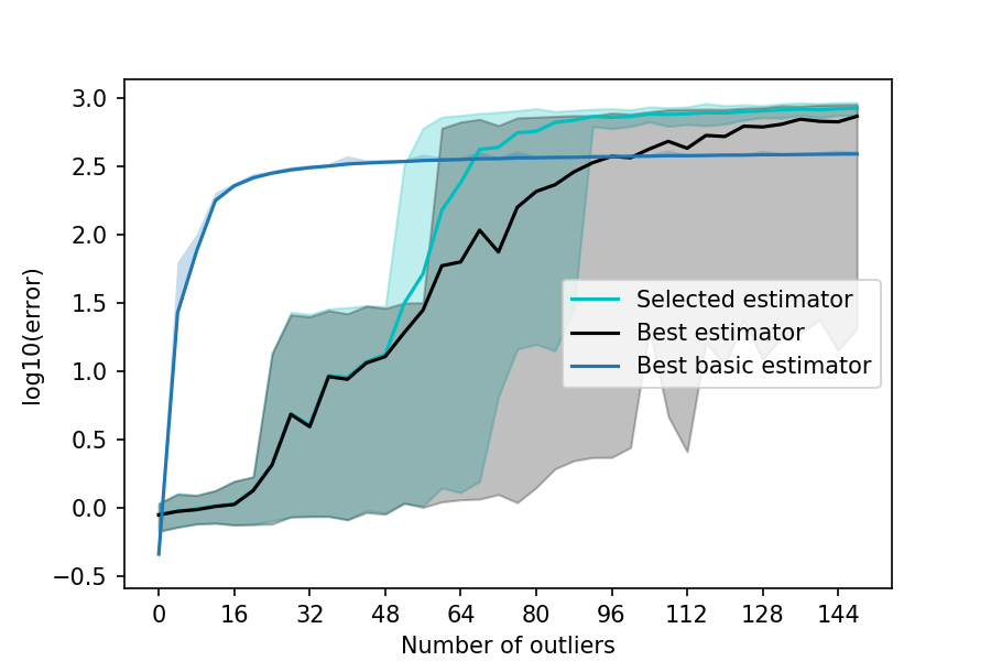
(a) Error of estimators $\hat{\beta}_{\widehat{m}}$, $\hat{\beta}_{\widetilde{m}}$ and $\hat{\beta}_{\widetilde{\lambda},[N]}$

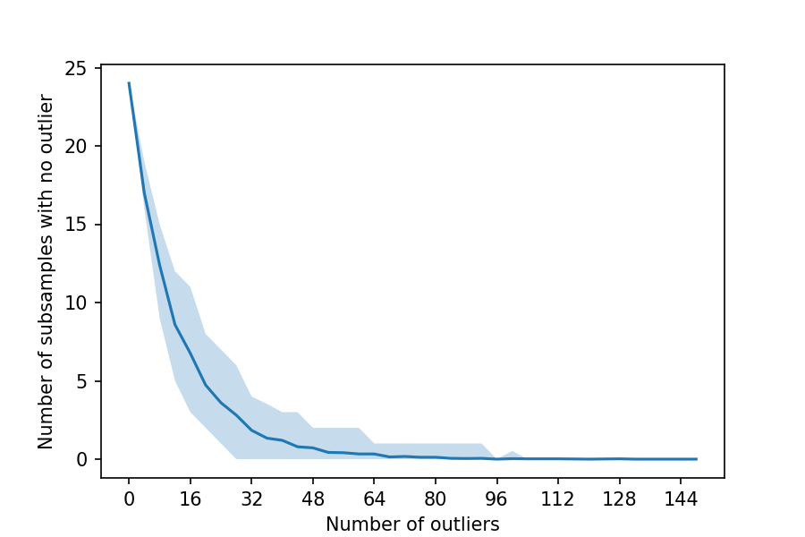
(b) Number of subsamples with no outlier

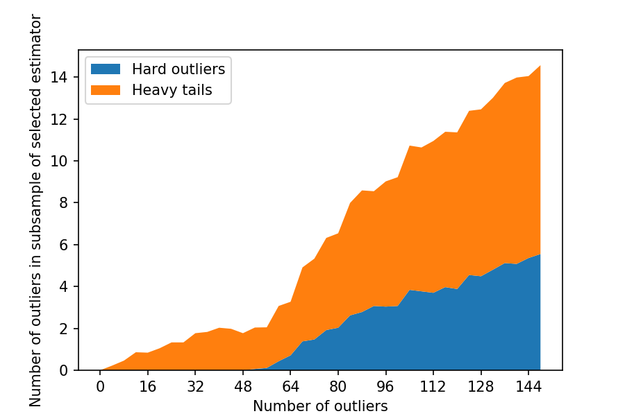
(c) Number of outliers in $B_{\widehat{m}}$

Figure 1: ensemble method run with $N=1000$, $V=40$, $K_{\text{max}}=4$, and averaged over 200 experiments.

The plots presented in Figure 1 are averaged over $100$ experiments. Figure 1(a) shows estimation error rates against the number $\left|\mathcal{O}\right|$ of outliers in the dataset and a $95\%$ confidence interval 1) of the output estimator $\hat{\beta}_{\widehat{m}}$ of the ensemble method, 2) of $\hat{\beta}_{\widetilde{m}}$, the best estimator among $(\hat{\beta}_{m})_{m\in\mathcal{M}}$, and 3) of the best basic estimator $\hat{\beta}_{\widetilde{\lambda},[N]}$. As soon as the dataset contains outliers, basic estimators $(\hat{\beta}_{\lambda,[N]})_{\lambda\in\Lambda}$ have larger errors than $\hat{\beta}_{\widetilde{m}}$ (the best estimator computed on a subsample). For $\left|\mathcal{O}\right|\leqslant 48$ the ensemble method procedure has the same error as the best estimator among $(\hat{\beta}_{m})_{m\in\mathcal{M}}$.

For a given value of parameter $V$, the minimax-MOM selection procedure (2) is expected to fail at some point when the number of outliers increases, but it seems here to resist to a much higher number of outliers than predicted by the theory. Theorem 3.2 holds for $\left|\mathcal{O}\right|\leqslant V/3$, that is $\left|\mathcal{O}\right|\leqslant 13$ here. It seems here that the minimax-MOM selection procedure performs satisfactorily for $\left|\mathcal{O}\right|\leqslant 48$ and even selects a reasonably good estimator for $\left|\mathcal{O}\right|\leqslant 56$.

Figure 1(c) shows the number of each type of outliers in the selected subsample $B_{\hat{m}}$. The method manages to rule out hard outliers when $\left|\mathcal{O}\right|\leqslant 48$, and the output estimator $\hat{\beta}_{\hat{m}}$ has in these cases minimal risk, as the best estimator $\hat{\beta}_{\widetilde{m}}$. Figure 1(b) also shows that almost all subsample contain outliers when $|{\cal O}|\geqslant 48$. Besides, the selected subsample $B_{\hat{m}}$ contains heavy-tail outliers even for small values of $\left|\mathcal{O}\right|$. As heavy-tail outliers and informative data define the same oracle, these heavy-tail outliers are actually informative for the learning task and the minimax-MOM selection procedure use this extra information automatically in an optimal way. In particular, the ensemble method distinguishes between non-informative hard outliers and possibly informative heavy-tailed outliers.

Overall, our method shows very strong robustness to the presence of outliers and outputs an estimator with the best possible performance among the given class of estimators.

Appendix A Application to ERM and linear aggregation

This section applies Corollary 4.1 by considering non-robust linear aggregation as input algorithms. Let $(F_{\lambda})_{\lambda\in\Lambda}$ be a finite collection of subspaces of $F$, typically spanned by previous estimators. For each $\lambda\in\Lambda$, denote by $d_{\lambda}$ the dimension of $F_{\lambda}$ and by $f^{*}_{\lambda}$ an oracle in $F_{\lambda}$, meaning $f_{\lambda}^{*}:=\operatorname*{arg\,min}_{f\in F_{\lambda}}R(f)$. Denote $\hat{f}_{\lambda,B}$ the empirical risk minimizer (ERM) on $F_{\lambda}$ trained with subsample $B$:

$$\hat{f}_{\lambda,B}:=\operatorname*{arg\,min}_{f\in F_{\lambda}}\frac{1}{\left|B\right|}\sum_{i\in B}(Y_{i}-f(X_{i}))^{2}.$$ (9)

The performance of ERM in linear aggregation like $\hat{f}_{\lambda,B}$ under a $L_{4}/L_{2}$ assumption such as Assumption 1 have been obtained in [31].

Proposition A.1 (Theorem 1.3 in [31]).

Let $\lambda\in\Lambda$. Assume that there exists $\chi_{\lambda}>0$ such that for all $f\in F_{\lambda}$, $(Pf^{4})^{1/4}\leqslant\chi_{\lambda}(Pf^{2})^{1/2}$. Denote $\zeta_{\lambda}:=Y-f_{\lambda}^{*}(X)$ and assume that $(P\zeta_{\lambda}^{4})^{1/4}\leqslant\sigma_{\lambda}$. Let $B\subset\mathcal{I}$ be such that $\left|B\right|\geqslant(1600\chi_{\lambda}^{4})^{2}d_{\lambda}$. Then, for every $x>0$, with probability larger than $1-\exp(-|B|/(64\chi_{\lambda}^{8}))-1/x$, the ERM $\hat{f}_{\lambda,B}$ defined in (9) satisfies

$$\ell(\hat{f}_{\lambda,B})\leqslant\ell(f_{\lambda}^{*})+(256)^{2}\chi_{\lambda}^{12}\frac{\sigma_{\lambda}^{2}d_{\lambda}x}{\left|B\right|}.$$

In Proposition A.1, the (exact) oracle inequality satisfied by $\hat{f}_{\lambda,B}$ guarantees an optimal residual term of order $\sigma_{\lambda}^{2}d_{\lambda}/N$ only when the deviation parameter $x$ is constant. This may seem weak, but it cannot be improved in general—see Proposition 1.5 in [31]: ERM are not robust to “stochastic outliers” in general.

We can now combine these algorithms with our ensemble method. Let $\mathcal{M}=\Lambda\times\mathcal{B}$ be as in (3) and $V$, $K_{\text{min}}$ and $K_{\text{max}}$ satisfy the assumptions from Section 4 and Corollary 4.1. Consider the output estimator $\hat{f}_{\widehat{m}}$ from (2). The following result combines Corollary 4.1 and Proposition A.1.

Corollary A.2.

Grant Assumption 1 on $F$ and assume that for all $\lambda\in\Lambda$ and all $f\in F_{\lambda}$, $(Pf^{4})^{1/4}\leqslant\chi_{\lambda}(Pf^{2})^{1/2}$ and $(P\zeta_{\lambda}^{4})^{1/4}\leqslant\sigma_{\lambda}$ for $\zeta_{\lambda}:=Y-f_{\lambda}^{*}(X)$. Assume also that $N\geqslant\max_{\lambda\in\Lambda}(1600\chi_{\lambda}^{4})^{2}d_{\lambda}\max(8V,2^{K_{\text{min}}+1})$. Then, with probability at least $1-(|\Lambda|^{2}N^{2}+1)\exp(-V/48)$, for all $\varepsilon>0$,

$$(1-a_{\varepsilon,V})\ell(\hat{f}_{\widehat{m}})\leqslant(1+3a_{\varepsilon,V})\times\min_{\lambda\in\Lambda}\left\{\ell(f_{\lambda}^{*})+2\exp(1/48)(256)^{2}\chi_{\lambda}^{12}\frac{\sigma_{\lambda}^{2}d_{\lambda}}{\lfloor N/\max(4V,2^{K_{\text{min}}})\rfloor}\right\}+2b_{\varepsilon,V}.$$

Proof.

The proof follows from Proposition A.1 and Corollary 4.1. Let us check the assumption and the features of both results. For $x=2\exp(1/48)$ and when $|B|\geqslant(1600\chi_{\lambda}^{4})^{2}d_{\lambda}$ we have $1-\exp(-|B|/(64\chi_{\lambda}^{8}))-1/x\geqslant 1-\exp(-1/48)$ therefore, $\hat{f}_{\lambda,B}$ satisfies an (exact) oracle inequality with probability larger than $1-\exp(-1/48)$ when $|B|\geqslant\nu(\lambda):=(1600\chi_{\lambda}^{4})^{2}d_{\lambda}$ with a residual term given by

$$\rho(\lambda,|B|)=\ell(f_{\lambda}^{*})+2(256)^{2}\exp(1/48)\chi_{\lambda}^{12}\frac{\sigma_{\lambda}^{2}d_{\lambda}}{\left|B\right|}.$$

Therefore, all the condition of Corollary 4.1 are satisfied and the result follows from a direct application of the latter result.  

Appendix B Lemmas and proofs

Let $\mathcal{V}^{(m,m^{\prime})}:=\left\{v\in[V]\,\middle|\,T_{v}^{(m,m^{\prime})}\subset\mathcal{I}\right\}$ denote the set of indices of blocks from the partition $(T_{v}^{(m,m^{\prime})}:v\in[V])$ containing only informative data. In particular, we have

$$\left|\mathcal{V}^{(m,m^{\prime})}\right|\geqslant V-\left|\mathcal{O}\right|.$$ (10)

Lemma B.1.

Let $m,m^{\prime}\in\mathcal{M}$ and $v\in\mathcal{V}^{(m,m^{\prime})}$. The conditional variance of random variable $P_{T_{v}^{(m,m^{\prime})}}\left[\gamma(\hat{f}_{m})-\gamma(\hat{f}_{m^{\prime}})\right]$ given random variables $(X_{i},Y_{i})_{i\in B_{m}\cup B_{m^{\prime}}}$ is bounded from above as:

$$\operatorname{Var}\left(P_{T_{v}^{(m,m^{\prime})}}\left[\gamma(\hat{f}_{m})-\gamma(\hat{f}_{m^{\prime}})\right]\,\middle|\,(X_{i},Y_{i})_{i\in B_{m}\cup B_{m^{\prime}}}\right)\leqslant C_{m,m^{\prime}},$$

where

$$C_{m,m^{\prime}}:=\frac{V}{N}\left(16\chi^{4}\left(\ell(\hat{f}_{m})^{2}+\ell(\hat{f}_{m^{\prime}})^{2}\right)+64\sigma^{2}\left(\ell(\hat{f}_{m})+\ell(\hat{f}_{m^{\prime}})\right)\right).$$

Proof.

By assumption, random variables $(X_{i},Y_{i})_{i\in\mathcal{I}}$ are independent. In particular, random variables $(X_{i},Y_{i})_{i\in T_{v}^{(m,m^{\prime})}}$ are independent conditionally to $(X_{i},Y_{i})_{i\in B_{m}\cup B_{m^{\prime}}}$ since $v\in\mathcal{V}^{(m,m^{\prime})}$. Using the shorthand notation $\operatorname{Var}_{m,m^{\prime}}(\,\cdot\,):=\operatorname{Var}\left(\,\cdot\,\,\middle|\,(X_{i},Y_{i})_{i\in B_{m}\cup B_{m^{\prime}}}\right)$, we have

$$\operatorname{Var}_{m,m^{\prime}}\left(P_{T_{v}^{(m,m^{\prime})}}\left[\gamma(\hat{f}_{m})-\gamma(\hat{f}_{m^{\prime}})\right]\right) =\operatorname{Var}_{m,m^{\prime}}\left(\frac{1}{\left|T_{v}^{(m,m^{\prime})}\right|}\sum_{i\in T_{v}^{(m,m^{\prime})}}(\gamma(\hat{f}_{m})-\gamma(\hat{f}_{m^{\prime}}))(X_{i},Y_{i})\right)$$

$$=\frac{1}{\left|T_{v}^{(m,m^{\prime})}\right|^{2}}\sum_{i\in T_{v}^{(m,m^{\prime})}}\operatorname{Var}_{m,m^{\prime}}\left((\gamma(\hat{f}_{m})-\gamma(\hat{f}_{m^{\prime}}))(X_{i},Y_{i})\right).$$

Fix $i\in T_{v}^{(m,m^{\prime})}\subset\mathcal{I}$, and let us bound from above each variance terms from the latter expression:

$$\operatorname{Var}_{m,m^{\prime}}\left((\gamma(\hat{f}_{m})-\gamma(\hat{f}_{m^{\prime}}))(X_{i},Y_{i})\right) \leqslant\mathbb{E}\left[\left((\gamma({\hat{f}_{m}})-\gamma(\hat{f}_{m^{\prime}}))(X_{i},Y_{i})\right)^{2}\,\middle|\,(X_{i^{\prime}},Y_{i^{\prime}})_{i^{\prime}\in B_{m}\cup B_{m^{\prime}}}\right]$$

$$=P\left[\left(\gamma(\hat{f}_{m})-\gamma(\hat{f}_{m^{\prime}})\right)^{2}\right]$$

$$=P\left[(\gamma(\hat{f}_{m})-\gamma(f^{*})+\gamma(f^{*})-\gamma(\hat{f}_{m^{\prime}}))^{2}\right]$$

$$\leqslant 2\,P\left[(\gamma(\hat{f}_{m})-\gamma(f^{*}))^{2}\right]+2\,P\left[(\gamma(\hat{f}_{m^{\prime}})-\gamma(f^{*}))^{2}\right],$$

where we used the basic inequality $(x+y)^{2}\leqslant 2(x^{2}+y^{2})$ in the last inequality. Let us bound from above the first term. The second term is handled similarly. We use a quadratic/multiplier decomposition of the excess loss:

$$P\left[(\gamma(\hat{f}_{m})-\gamma(f^{*}))^{2}\right] =P\left[\left(\left(\hat{f}_{m}-f^{*}\right)^{2}-2(Y-f^{*})(\hat{f}_{m}-f^{*})\right)^{2}\right]$$

$$\leqslant 2P\left[(\hat{f}_{m}-f^{*})^{4}\right]+8P\left[(Y-f^{*})^{2}(\hat{f}_{m}-f^{*})^{2}\right].$$

By Assumption 1, it follows that

$$P\left[(\hat{f}_{m}-f^{*})^{4}\right]\leqslant\chi^{4}\left(P\left[(\hat{f}_{m}-f^{*})^{2}\right]\right)^{2}=\chi^{4}\ \ell(\hat{f}_{m})^{2}.$$

Likewise, Assumption 1 yields

$$P\left[(Y-f^{*})^{2}(\hat{f}_{m}-f^{*})^{2}\right]\leqslant\sigma^{2}P\left[(\hat{f}_{m}-f^{*})^{2}\right]=\sigma^{2}\ell(\hat{f}_{m}).$$

The result follows from combining these pieces and using $\left|T_{v}^{(m,m^{\prime})}\right|\geqslant N/4V$.  

Lemma B.2.

With probability higher than $1-\left|\mathcal{M}\right|^{2}e^{-(V-\left|\mathcal{O}\right|)/32}$, for all $m,m^{\prime}\in\mathcal{M}$,

$$\ell(\hat{f}_{m})-\ell(\hat{f}_{m^{\prime}})-\sqrt{8\,C_{m,m^{\prime}}}\leqslant\mathcal{T}(m,m^{\prime})\leqslant\ell(\hat{f}_{m})-\ell(\hat{f}_{m^{\prime}})+\sqrt{8\,C_{m,m^{\prime}}}$$

where $\mathcal{T}(m,m^{\prime}):=\operatorname*{med}_{v\in[V]}\left\{P_{T_{v}^{(m,m^{\prime})}}\left[\gamma(\hat{f}_{m})-\gamma(\hat{f}_{m^{\prime}})\right]\right\}$.

Proof.

Fix $m,m^{\prime}\in\mathcal{M}$ and $v\in\mathcal{V}^{(m,m^{\prime})}$. Conditionally to $(X_{i},Y_{i})_{i\in B_{m}\cup B_{m^{\prime}}}$, it follows from Chebychev’s inequality and Lemma B.1 that, with probability higher than $1-1/8$,

$$\left|P_{T_{v}^{(m,m^{\prime})}}\left[\gamma(\hat{f}_{m})-\gamma({\hat{f}_{m^{\prime}}})\right]-(\ell(\hat{f}_{m})-\ell(\hat{f}_{m^{\prime}}))\right|$$

$$\leqslant\sqrt{8\operatorname{Var}\left(P_{T_{v}^{(m,m^{\prime})}}\left[\gamma({\hat{f}_{m}})-\gamma({\hat{f}_{m^{\prime}}})\right]\,\middle|\,(X_{i},Y_{i})_{i\in B_{m}\cup B_{m^{\prime}}}\right)}$$

$$\leqslant\sqrt{8\,C_{m,m^{\prime}}}.$$

As the probability estimate does not depend on$(X_{i},Y_{i})_{i\in B_{m}\cup B_{m^{\prime}}}$, the above also holds unconditionnally and, with probability larger than $1-1/8$,

$$\ell(\hat{f}_{m})-\ell(\hat{f}_{m^{\prime}})-\sqrt{8\,C_{m,m^{\prime}}}\leqslant P_{T_{v}^{(m,m^{\prime})}}\left[\gamma({\hat{f}_{m}})-\gamma({\hat{f}_{m^{\prime}}})\right]\leqslant\ell(\hat{f}_{m})-\ell(\hat{f}_{m^{\prime}})+\sqrt{8\,C_{m,m^{\prime}}}.$$ (11)

Denote by $\Omega_{v}^{(m,m^{\prime})}$ the event defined by (11) and see that $\mathbb{P}\left[\Omega_{v}^{(m,m^{\prime})}\right]\geqslant 1-1/8$. Apply now Hoeffding’s inequality to random variables $\mathbbm{1}_{\Omega_{v}^{(m,m^{\prime})}},v\in\mathcal{V}^{(m,m^{\prime})}$ which are independent conditionnally to $(X_{i},Y_{i})_{B_{m}\cup B_{m^{\prime}}}$: on an event $\Omega^{(m,m^{\prime})}$ of probability larger than $1-e^{-2\left|\mathcal{V}^{(m,m^{\prime})}\right|(1/8)^{2}}\geqslant 1-e^{-(V-\left|\mathcal{O}\right|)/32}$, see (10),

$$\frac{1}{\left|\mathcal{V}^{(m,m^{\prime})}\right|}\sum_{v\in\mathcal{V}^{(m,m^{\prime})}}\mathbbm{1}_{\Omega_{v}^{(m,m^{\prime})}} \geqslant\mathbb{E}\left[\frac{1}{\left|\mathcal{V}^{(m,m^{\prime})}\right|}\sum_{v\in\mathcal{V}^{(m,m^{\prime})}}\mathbbm{1}_{\Omega_{v}^{(m,m^{\prime})}}\right]-\frac{1}{8}$$

$$=\frac{1}{\left|\mathcal{V}^{(m,m^{\prime})}\right|}\sum_{v\in\mathcal{V}^{(m,m^{\prime})}}\mathbb{P}\left[\Omega_{v}^{(m,m^{\prime})}\right]-\frac{1}{8}\geqslant\frac{3}{4}.$$

Then, on $\Omega^{(m,m^{\prime})}$, using (10) and the assumption $V\geqslant 3|{\cal O}|$,

$$\sum_{v\in\mathcal{V}^{(m,m^{\prime})}}\mathbbm{1}_{\Omega_{v}^{(m,m^{\prime})}}\geqslant\frac{3}{4}\left|\mathcal{V}^{(m,m^{\prime})}\right|\geqslant\frac{3}{4}\left(V-\left|\mathcal{O}\right|\right)\geqslant\frac{V}{2}.$$

In other words, inequalities (11) hold for more than half of the indices $v\in[V]$. Therefore, on event $\Omega^{(m,m^{\prime})}$, the same inequality holds for the median over $v\in[V]$:

$$\ell(\hat{f}_{m})-\ell(\hat{f}_{m^{\prime}})-\sqrt{8C_{m,m^{\prime}}}\leqslant\mathcal{T}(m,m^{\prime})\leqslant\ell(\hat{f}_{m})-\ell(\hat{f}_{m^{\prime}})+\sqrt{8\,C_{m,m^{\prime}}}.$$

By a union bound, the above holds for all $m,m^{\prime}\in\mathcal{M}$ with probability at least $1-\left|\mathcal{M}\right|^{2}e^{-(V-\left|\mathcal{O}\right|)/32}$.  

Lemma B.3.

For all $m,m^{\prime}\in\mathcal{M}$, $\varepsilon^{\prime}>0$ and $b>0$,

$$\sqrt{8\,C_{m,m^{\prime}}}\leqslant\sqrt{\frac{8V}{N}}\left((4\chi^{2}+\varepsilon^{\prime})(\ell(\hat{f}_{m})+\ell(\hat{f}_{m^{\prime}}))+\frac{16\sigma^{2}}{\varepsilon^{\prime}}\right).$$

Proof.

By definition of $C_{m,m^{\prime}}$ and the inequalities $\sqrt{x+y}\leqslant\sqrt{x}+\sqrt{y}$ and $2xy\leqslant x^{2}/\varepsilon^{\prime}+\varepsilon^{\prime}y^{2}$,

$$\sqrt{8C_{m,m^{\prime}}} =\sqrt{\frac{8V}{N}\left(16\chi^{4}\left(\ell(\hat{f}_{m})^{2}+\ell(\hat{f}_{m^{\prime}})^{2}\right)+64\sigma^{2}\left(\ell(\hat{f}_{m})+\ell(\hat{f}_{m^{\prime}})\right)\right)}$$

$$\leqslant\sqrt{\frac{8V}{N}}\left(4\chi^{2}\sqrt{\ell(\hat{f}_{m})^{2}+\ell(\hat{f}_{m^{\prime}})^{2}}+8\sigma\sqrt{\ell(\hat{f}_{m})+\ell(\hat{f}_{m^{\prime}})}\right),$$

$$\leqslant\sqrt{\frac{8V}{N}}\left(4\chi^{2}(\ell(\hat{f}_{m})+\ell(\hat{f}_{m^{\prime}}))+\frac{16\sigma^{2}}{\varepsilon^{\prime}}+\varepsilon^{\prime}(\ell(\hat{f}_{m})+\ell(\hat{f}_{m^{\prime}}))\right)$$

$$=\sqrt{\frac{8V}{N}}\left((4\chi^{2}+\varepsilon^{\prime})(\ell(\hat{f}_{m})+\ell(\hat{f}_{m^{\prime}}))+\frac{16\sigma^{2}}{\varepsilon^{\prime}}\right).$$

 

Lemma B.4.

With probability at least $1-\left|\mathcal{M}\right|^{2}e^{-(V-\left|\mathcal{O}\right|)/32}$, for all $m,m^{\prime}\in\mathcal{M}$ and $\varepsilon>0$:

$$(1-a_{\varepsilon,V})\ell(\hat{f}_{m})-(1+a_{\varepsilon,V})\ell(\hat{f}_{m^{\prime}})-b_{\varepsilon,V}\leqslant\mathcal{T}(m,m^{\prime})\leqslant(1+a_{\varepsilon,V})\ell(\hat{f}_{m})-(1-a_{\varepsilon,V})\ell(\hat{f}_{m^{\prime}})+b_{\varepsilon,V}.$$

Proof.

The result follows from Lemmas B.2 and B.3 for $\varepsilon^{\prime}=\sqrt{N/V}\varepsilon$, together with the definition of $a_{\varepsilon,V}$ and $b_{\varepsilon,V}$.  

Appendix C Proofs of the main results

C.1 Proof of Theorem 3.2

Assume that $a_{\varepsilon,V}<1$, otherwise the result is trivial. Denote $m_{o}:=\operatorname*{arg\,min}_{m\in\mathcal{M}}\ell(\hat{f}_{m})$, so

$$(1-a_{\varepsilon,V})\ell(\hat{f}_{\widehat{m}})=(1-a_{\varepsilon,V})\ell(\hat{f}_{\widehat{m}})-(1+a_{\varepsilon,V})\ell(\hat{f}_{m_{o}})+(1+a_{\varepsilon,V})\ell(\hat{f}_{m_{o}}).$$ (12)

Let $\Omega$ be the event defined by Lemma B.4. Since $V\geqslant 3|{\cal O}|$, by Lemma B.4

$${\mathbb{P}}\left(\Omega\right)\geqslant 1-\left|\mathcal{M}\right|^{2}e^{-(V-\left|\mathcal{O}\right|)/32}\geqslant 1-\left|\mathcal{M}\right|^{2}e^{-V/48}\enspace.$$

It follows from Lemma B.4 and (12) that, on $\Omega$,

$$(1-a_{\varepsilon,V})\ell(\hat{f}_{\widehat{m}})\leqslant\max_{m\in\mathcal{M}}\mathcal{T}(\hat{m},m)+b_{\varepsilon,V}+(1+a_{\varepsilon,V})\ell(\hat{f}_{m_{o}}).$$ (13)

Then, by definition of $\hat{m}$ and using Lemma B.4, on $\Omega$,

$$\max_{m\in\mathcal{M}}\mathcal{T}(\hat{m},m) =\min_{m^{\prime}\in\mathcal{M}}\max_{m\in\mathcal{M}}\mathcal{T}(m^{\prime},m)\leqslant\max_{m\in\mathcal{M}}\mathcal{T}(m_{o},m)$$

$$\leqslant\max_{m\in\mathcal{M}}\left\{(1+a_{\varepsilon,V})\ell(\hat{f}_{m_{o}})-(1-a_{\varepsilon,V})\ell(\hat{f}_{m})+b_{\varepsilon,V}\right\}$$

$$=(1+a_{\varepsilon,V})\ell(\hat{f}_{m_{o}})-(1-a_{\varepsilon,V})\ell(\hat{f}_{m_{o}})+b_{\varepsilon,V}=2a_{\varepsilon,V}\ell(\hat{f}_{m_{o}})+b_{\varepsilon,V},$$

where we used $1-a_{\varepsilon,V}\geqslant 0$ and the definition of $m_{o}$. Plugging this into (13) yields the result.

C.2 Proof of Corollary 4.1

Let

$$K_{0}:=\max\left(\left\lceil\log_{2}(2V)\right\rceil,K_{\text{min}}\right).$$

It follows from the assumption $V\leqslant 2^{K_{\text{max}}-1}$ that $K_{0}\in\left\llbracket K_{\text{min}},K_{\text{max}}\right\rrbracket$. Besides, it follows from the above definition that:

$$2^{K_{0}}\leqslant\max(4V,2^{K_{\text{min}}}).$$ (14)

Let also

$$\lambda_{0}:=\operatorname*{arg\,min}_{\lambda\in\Lambda}\rho(\lambda,\lfloor N/2^{K_{0}}\rfloor)\qquad\text{and}\qquad\rho_{0}:=\rho(\lambda_{0},\lfloor N/2^{K_{0}}\rfloor).$$

$$\mathcal{K}_{0}:=\left\{k\in[2^{K_{0}}]\,\middle|\,B_{k}^{(K_{0})}\subset\mathcal{I}\right\},$$

which is nonempty because $\left|\mathcal{K}_{0}\right|\geqslant 2^{K_{0}}-\left|\mathcal{O}\right|\geqslant 2V-\left|\mathcal{O}\right|\geqslant 2V-V/3\geqslant V$, where the first inequality follows from the definition of $\mathcal{K}_{0}$, the second inequality from the definition of $K_{0}$ and the third inequality from the assumption $V\geqslant 3\left|\mathcal{O}\right|$.

Consider the events

$$\Omega_{1} =\left\{(1-a_{\varepsilon,V})\ell(\hat{f}_{\widehat{m}})\leqslant(1+3a_{\varepsilon,V})\min_{m\in\mathcal{M}}\ell(\hat{f}_{m})+2b_{\varepsilon,V}\right\}$$

$$\Omega_{2} =\left\{\exists k\in\mathcal{K}_{0},\ \ell\left(\hat{f}_{\lambda_{0},B_{k}^{(K_{0})}}\right)\leqslant\rho_{0}\right\}.$$

From now on, assume that $\Omega_{1}\cap\Omega_{2}$ hold and the aim is to establish an upper bound on $\min_{m\in\mathcal{M}}\ell(\hat{f}_{m})$. Write

$$\min_{m\in\mathcal{M}}\ell(\hat{f}_{m})=\min_{\begin{subarray}{c}\lambda\in\Lambda\\ B\in\mathcal{B}\end{subarray}}\ell(\hat{f}_{\lambda,B})\leqslant\min_{k\in\mathcal{K}_{0}}\ell\left(\hat{f}_{\lambda_{0},B_{k}^{(K_{0})}}\right) \leqslant\rho_{0}=\min_{\lambda\in\Lambda}\rho(\lambda,\lfloor N/2^{K_{0}}\rfloor)$$

$$\leqslant\min_{\lambda\in\Lambda}\rho\left(\lambda,\left\lfloor\frac{N}{\max(4V,2^{K_{\text{min}}})}\right\rfloor\right).$$

Here the second inequality comes from the definition of $\Omega_{2}$ and the last inequality from (14) combined with $\rho$ being nonincreasing in its second variable. Combining the above with the definition of $\Omega_{1}$ yields the desired inequality:

$$(1-a_{\varepsilon,V})\ell(\hat{f}_{\widehat{m}})\leqslant(1+3a_{\varepsilon,V})\,\min_{\lambda\in\Lambda}\rho\left(\lambda,\left\lfloor\frac{N}{\max(4V,2^{K_{\text{min}}})}\right\rfloor\right)+2b_{\varepsilon,V}.$$

To conclude the proof, let us bound from below the probability of $\Omega_{1}\cap\Omega_{2}$. By Theorem 3.2,

$$\mathbb{P}\left[\Omega_{1}\cap\Omega_{2}\right] =1-\mathbb{P}\left[\Omega_{1}^{c}\cup\Omega_{2}^{c}\right]\geqslant 1-\mathbb{P}\left[\Omega_{1}^{c}\right]-\mathbb{P}\left[\Omega_{2}^{c}\right]$$

$$\geqslant 1-\left|\mathcal{M}\right|^{2}e^{-V/48}-\mathbb{P}\left[\Omega_{2}^{c}\right]\geqslant 1-\left|\Lambda\right|^{2}N^{2}e^{-V/48}-\mathbb{P}\left[\Omega_{2}^{c}\right],$$

Recall that $\lfloor N/2^{K_{0}}\rfloor\leqslant\left|B_{k}^{(K_{0})}\right|$ for all $k\in\left[2^{K_{0}}\right]$, that $\rho$ is non-increasing in its second variable and that $B_{k}^{(K_{0})},k\in{\cal K}_{0}$ are disjoint, so

$$\mathbb{P}\left[\Omega_{2}^{c}\right] =\mathbb{P}\left[\forall k\in\mathcal{K}_{0},\ \ell\left(\hat{f}_{\lambda_{0},B_{k}^{(K_{0})}}\right)>\rho_{0}\right]=\prod_{k\in\mathcal{K}_{0}}\mathbb{P}\left[\ell\left(\hat{f}_{\lambda_{0},B_{k}^{(K_{0})}}\right)>\rho_{0}\right]$$

$$\leqslant\prod_{k\in\mathcal{K}_{0}}\mathbb{P}\left[\ell\left(\hat{f}_{\lambda_{0},B_{k}^{(K_{0})}}\right)>\rho\left(\lambda_{0},\left|B_{k}^{(K_{0})}\right|\right)\right]$$

$$\leqslant\exp(-|{\cal K}_{0}|/48)\leqslant\exp(-V/48)\enspace.$$

The third inequality follows from the excess risk bound on $\hat{f}_{\lambda_{0},B_{k}^{(K_{0})}}$, which holds as soon as $\left|B_{k}^{(K_{0})}\right|\geqslant\nu(\lambda_{0})$; this is indeed case because using (14):

$$\left|B_{k}^{(K_{0})}\right|\geqslant\left\lfloor\frac{N}{2^{K_{0}}}\right\rfloor \geqslant\left\lfloor\frac{N}{\max(4V,2^{K_{\text{min}}})}\right\rfloor=\frac{N}{2\max(2V,2^{K_{\text{min}}})}\geqslant\nu_{\text{max}}\geqslant\nu(\lambda_{0}),$$

where the penultimate inequality follows from assumption $N\geqslant\nu_{\text{max}}\max(8V,2^{K_{\text{min}}+1})$. Therefore, $\mathbb{P}\left[\Omega_{1}\cap\Omega_{2}\right]\geqslant 1-(\left|\Lambda\right|^{2}N^{2}+1)\exp(-V/48)$.

C.3 Proof of Lemma 4.2

Start with (i). Let $k\in[2^{K}]$ and $i\in B_{k}^{(K)}$, which by definition of $B_{k}^{(K)}$ means:

$$\left\lfloor\frac{(k-1)N}{2^{K}}\right\rfloor<i\leqslant\left\lfloor\frac{kN}{2^{K}}\right\rfloor.$$

We can bound from below as follows: let $k^{\prime}:=\lfloor(k-1)(2^{K^{\prime}-K})\rfloor+1$,

$$\left\lfloor\frac{(k-1)N}{2^{K}}\right\rfloor=\left\lfloor\frac{(k-1)(2^{K^{\prime}-K})N}{2^{K^{\prime}}}\right\rfloor\geqslant\left\lfloor\frac{\lfloor(k-1)(2^{K^{\prime}-K})\rfloor N}{2^{K}}\right\rfloor=\left\lfloor\frac{(k^{\prime}-1)N}{2^{K}}\right\rfloor.$$

Similarly, the upper bound is obtained as follows:

$$\left\lfloor\frac{kN}{2^{K}}\right\rfloor =\left\lfloor\frac{((k-1)2^{K^{\prime}-K}+2^{K^{\prime}-K})N}{2^{K^{\prime}}}\right\rfloor\leqslant\left\lfloor\frac{((k-1)2^{K^{\prime}-K}+2)N}{2^{K^{\prime}}}\right\rfloor$$

$$\leqslant\left\lfloor\frac{(\lfloor(k-1)2^{K^{\prime}-K}\rfloor+1)N}{2^{K^{\prime}}}\right\rfloor=\left\lfloor\frac{k^{\prime}N}{2^{K^{\prime}}}\right\rfloor.$$

Therefore,

$$\left\lfloor\frac{(k^{\prime}-1)N}{2^{K^{\prime}}}\right\rfloor<i\leqslant\left\lfloor\frac{k^{\prime}N}{2^{K^{\prime}}}\right\rfloor.$$

This means $i\in B_{\lfloor(k-1)2^{K^{\prime}-K}\rfloor+1}^{(K^{\prime})}$.

The proof of (ii) proceeds as follows. Let $k^{\prime}\in[2^{K^{\prime}}]$ and $i\in B_{k^{\prime}}^{(K^{\prime})}$, meaning that

$$\left\lfloor\frac{(k^{\prime}-1)N}{2^{K^{\prime}}}\right\rfloor<i\leqslant\left\lfloor\frac{k^{\prime}N}{2^{K^{\prime}}}\right\rfloor.$$

This can be rewritten as

$$\left\lfloor\frac{2^{K-K^{\prime}}(k^{\prime}-1)N}{2^{K}}\right\rfloor<i\leqslant\left\lfloor\frac{2^{K-K^{\prime}}k^{\prime}N}{2^{K}}\right\rfloor,$$

As $(B_{k}^{(K)})_{k\in[2^{K}]}$ is a partition of $[N]$, there exists a unique $k\in[2^{K}]$ such that $i\in B_{k}^{(K)}$, i.e.

$$\left\lfloor\frac{(k-1)N}{2^{K}}\right\rfloor<i\leqslant\left\lfloor\frac{kN}{2^{K}}\right\rfloor.$$

Combining the two previous displays implies that $(k^{\prime}-1)2^{K-K^{\prime}}<k\leqslant k^{\prime}2^{K-K^{\prime}}$, meaning that $i\in B_{k}^{(K)}$. Moreover, applying (i) to $k$ gives that $B_{k}^{(K)}$ is a subset of $B_{k^{\prime}}^{(K^{\prime})}$, hence the result.

C.4 Proof of Lemma 4.3

Using (i) from Lemma 4.2, we have:

$$B_{k_{1}}^{K_{1}} \subset B_{k_{1}^{\prime}}^{(3)},\quad\text{with}\quad k_{1}^{\prime}=\lfloor(k_{1}-1)2^{3-K_{1}}\rfloor+1,$$

$$B_{k_{2}}^{K_{2}} \subset B_{k_{2}^{\prime}}^{(3)},\quad\text{with}\quad k_{2}^{\prime}=\lfloor(k_{2}-1)2^{3-K_{2}}\rfloor+1.$$

In addition, $K_{0}$ is by definition larger than $3$ (see (6)) and (ii) from Lemma 4.3 then gives:

$$(B_{k}^{(K_{0})})_{k\in\left\rrbracket(k_{1}^{\prime}-1)2^{K_{0}-3},\ k_{1}^{\prime}2^{K_{0}-3}\right\rrbracket} \quad\text{is a partition of}\quad B_{k_{1}^{\prime}}^{(3)},$$

$$(B_{k}^{(K_{0})})_{k\in\left\rrbracket(k_{2}^{\prime}-1)2^{K_{0}-3},\ k_{2}^{\prime}2^{K_{0}-3}\right\rrbracket} \quad\text{ is a partition of }\quad B_{k_{2}^{\prime}}^{(3)}.$$

Then, using the latter result and starting from the definition of $\mathcal{K}_{0}(K_{1},k_{1},K_{2},k_{2})$, we can write

$$\mathcal{K}_{0}(K_{1},k_{1},K_{2},k_{2}) =\left\{k\in\left[2^{K_{0}}\right]\,\middle|\,B_{k}^{(K_{0})}\cap(B_{k_{1}}^{(K_{1})}\cup B_{k_{2}}^{(K_{2})})=\varnothing\right\}$$

$$\supset\left\{k\in\left[2^{K_{0}}\right]\,\middle|\,B_{k}^{(K_{0})}\cap(B_{k_{1}^{\prime}}^{(3)}\cup B_{k_{2}^{\prime}}^{(3)})=\varnothing\right\}$$

$$=\left[2^{K_{0}}\right]\setminus\left(\left\rrbracket(k_{1}^{\prime}-1)2^{K_{0}-3},\ k_{1}^{\prime}2^{K_{0}-3}\right\rrbracket\cup\left\rrbracket(k_{2}^{\prime}-1)2^{K_{0}-3},\ k_{2}^{\prime}2^{K_{0}-3}\right\rrbracket\right).$$

The latter result together with the definition of $K_{0}$ yield the lower bound on the cardinality of $\mathcal{K}_{0}(k_{1},K_{1},K_{2},k_{2})$:

$$\left|\mathcal{K}_{0}(K_{1},k_{1},K_{2},k_{2})\right| \geqslant 2^{K_{0}}-2^{K_{0}-3}-2^{K_{0}-3}=\frac{3}{4}2^{K_{0}}\geqslant\frac{3}{4}2^{\log_{2}(V/3)+2}=V.$$

C.5 Proof of Lemma 4.4

Let $(m,m^{\prime})\in\mathcal{M}^{2}$ and $v\in[V]$. By construction of $T_{v}^{(m,m^{\prime})}$, there exists $k\in\left[2^{K_{0}}\right]$ such that $T_{v}^{(m,m^{\prime})}=B_{k}^{(K_{0})}$. Then, it follows from (6) that $2^{K_{0}}\leqslant 8V/3$, so that we can write:

$$\left|T_{v}^{(m,m^{\prime})}\right|\geqslant\left\lfloor\frac{N}{2^{K_{0}}}\right\rfloor\geqslant\left\lfloor\frac{3N}{8V}\right\rfloor=\left\lfloor\frac{N}{4V}+\frac{N}{8V}\right\rfloor\geqslant\left\lfloor\frac{N}{4V}+1\right\rfloor\geqslant\frac{N}{4V},$$

where we used the fact that $V\leqslant N/8$ by assumption.

C.6 Proof of Corollary 5.2

Let us apply Corollary 4.1 with well-chosen functions $\nu\colon\lambda\to\mathbb{R}_{+}^{*}$ and $\rho\colon\Lambda\times\mathbb{N}^{*}\to\mathbb{R}_{+}\cup\left\{+\infty\right\}$. For $s\in[s^{*}]$, denote,

$$\lambda_{s}=c_{0}\left\|\zeta\right\|_{L_{q}}\sqrt{s\log(ed/s)}$$

so that $\Lambda=\left\{\lambda_{s}\right\}_{s\in[s^{*}]}$. For $s\in[s^{*}]$, we define

$$\nu(\lambda_{s})=s\log(ed/s).$$

Then, by definition of $s^{*}$, we get $\nu_{\text{max}}=\left\lceil\max_{\lambda\in\Lambda}\nu(\lambda)\right\rceil=\left\lceil s^{*}\log(ed/s^{*})\right\rceil$, and the assumption $N/(8V,2^{K_{\text{min}}+1})\geqslant s_{*}\log(ed/s^{*})$ implies $N\geqslant\nu_{\text{max}}\max(8V,2^{K_{\text{min}}+1})$ which is required to apply Corollary 4.1. Besides, we define $\rho$ as follows. For $s\in[s^{*}]$ and $c\in\mathbb{N}^{*}$,

$$\rho(\lambda_{s},c)=\begin{cases}\lambda_{s}^{2}c_{1}c_{0}^{-2}c^{-1}&\text{if $s\geqslant\left\|\beta^{*}\right\|_{0}$}\\ +\infty&\text{otherwise}.\end{cases}$$

For all $s\geqslant\left\|\beta^{*}\right\|_{0}$, $\beta^{*}$ is of course $s$-sparse, and then according to Proposition 5.1, for $B\subset\mathcal{I}$ such that $\left|B\right|\geqslant\nu(\lambda_{s})$, it holds with probability higher than $1-e^{-1/48}$ that

$$\ell(\hat{f}_{\lambda_{s},B})=\ell(\hat{\beta}_{\lambda_{s}\left|B\right|^{-1/2},B})\leqslant\rho(\lambda_{s},\left|B\right|).$$

The above inequality is also true for $s<\left\|\beta^{*}\right\|_{0}$ since the right-hand side is then infinite. We can now apply Corollary 4.1 which gives that with probability higher than $1-((s^{*})^{2}N^{2}+1)e^{-V/48}$, it holds that:

$$(1-a_{\varepsilon,V})\ell(\hat{f}_{\widehat{m}})\leqslant(1+3a_{\varepsilon,V})\,\min_{\lambda\in\Lambda}\rho\left(\lambda,\left\lfloor\frac{N}{\max(4V,2^{K_{\text{min}}})}\right\rfloor\right)+2b_{\varepsilon,V},$$

and the result follows by noting that:

$$\min_{\lambda\in\Lambda}\rho\left(\lambda,\left\lfloor\frac{N}{\max(4V,2^{K_{\text{min}}})}\right\rfloor\right) =\min_{s\in[s^{*}]}\rho\left(\lambda_{s},\ \left\lfloor\frac{N}{\max(4V,2^{K_{\text{min}}})}\right\rfloor\right)$$

$$=\min_{s\geqslant\left\|\beta^{*}\right\|_{0}}\lambda_{s}^{2}c_{1}c_{0}^{-2}\left\lfloor\frac{N}{\max(4V,2^{K_{\text{min}}})}\right\rfloor^{-1}$$

$$=\min_{s\geqslant\left\|\beta^{*}\right\|_{0}}\left\|\zeta\right\|_{L_{q}}^{2}s\log(ed/s)c_{1}\left\lfloor\frac{N}{\max(4V,2^{K_{\text{min}}})}\right\rfloor^{-1}$$

$$=c_{1}\left\|\zeta\right\|_{L_{q}}^{2}\frac{\left\|\beta^{*}\right\|_{0}\log(ed\left\|\beta^{*}\right\|_{0}^{-1})}{\left\lfloor N/\max(4V,2^{K_{\text{min}}})\right\rfloor}.$$

References

- [1] Noga Alon, Yossi Matias, and Mario Szegedy. The space complexity of approximating the frequency moments. J. Comput. System Sci., 58(1, part 2):137–147, 1999. Twenty-eighth Annual ACM Symposium on the Theory of Computing (Philadelphia, PA, 1996).
- [2] S. Arlot and A. Celisse. A survey of cross-validation procedures for model selection. Stat. Surv., 4:40–79, 2010.
- [3] S. Arlot and M. Lerasle. Choice of for -fold cross-validation in least-squares density estimation. J. Mach. Learn. Res., 17:Paper No. 208, 50, 2016.
- [4] Jean-Yves Audibert and Olivier Catoni. Robust linear least squares regression. Ann. Statist., 39(5):2766–2794, 2011.
- [5] Y. Baraud, L. Birgé, and M. Sart. A new method for estimation and model selection: -estimation. Invent. Math., 207(2):425–517, 2017.
- [6] Yannick Baraud. Estimator selection with respect to Hellinger-type risks. Probab. Theory Related Fields, 151(1-2):353–401, 2011.
- [7] Yannick Baraud, Christophe Giraud, and Sylvie Huet. Estimator selection in the Gaussian setting. Ann. Inst. Henri Poincaré Probab. Stat., 50(3):1092–1119, 2014.
- [8] Andrew Barron, Lucien Birgé, and Pascal Massart. Risk bounds for model selection via penalization. Probab. Theory Related Fields, 113(3):301–413, 1999.
- [9] Pierre C. Bellec. Optimal bounds for aggregation of affine estimators. Ann. Statist., 46(1):30–59, 2018.
- [10] Pierre C Bellec, Guillaume Lecué, Alexandre B Tsybakov, et al. Slope meets lasso: improved oracle bounds and optimality. The Annals of Statistics, 46(6B):3603–3642, 2018.
- [11] Lucien Birgé and Pascal Massart. From model selection to adaptive estimation. In Festschrift for Lucien Le Cam, pages 55–87. Springer, New York, 1997.
- [12] Lucien Birgé and Pascal Massart. Gaussian model selection. J. Eur. Math. Soc. (JEMS), 3(3):203–268, 2001.
- [13] Jelena Bradic. Randomized maximum-contrast selection: subagging for large-scale regression. Electronic Journal of Statistics, 10(1):121–170, 2016.
- [14] Leo Breiman. Bagging Predictors. Machine Learning, 24(2):123–140, 1996.
- [15] Peter Bühlmann. Bagging, subagging and bragging for improving some prediction algorithms. In Recent advances and trends in nonparametric statistics, pages 19–34. Elsevier B. V., Amsterdam, 2003.
- [16] Olivier Catoni. Statistical learning theory and stochastic optimization, volume 1851 of Lecture Notes in Mathematics. Springer-Verlag, Berlin, 2004. Lecture notes from the 31st Summer School on Probability Theory held in Saint-Flour, July 8–25, 2001.
- [17] Xueying Chen and Min-ge Xie. A split-and-conquer approach for analysis of extraordinarily large data. Statistica Sinica, 24:1655–1684, 2014.
- [18] Jeffrey Dean and Sanjay Ghemawat. Mapreduce: simplified data processing on large clusters. Communications of the ACM, 51(1):107–113, 2008.
- [19] David L. Donoho and Iain M. Johnstone. Ideal spatial adaptation by wavelet shrinkage. Biometrika, 81(3):425–455, 1994.
- [20] J. Fan, Q. Li, and Y. Wang. Estimation of high-dimensional mean regression in absence of symmetry and light-tail assumptions. Journal of Royal Statistical Society B, 79:247–265, 2017.
- [21] A. Goldenshluger and O. Lepski. Universal pointwise selection rule in multivariate function estimation. Bernoulli, 14(4):1150–1190, 11 2008.
- [22] Matthew J Holland. Classification using margin pursuit. arXiv preprint arXiv:1810.04863, 2018.
- [23] Matthew J Holland. Robust descent using smoothed multiplicative noise. arXiv preprint arXiv:1810.06207, 2018.
- [24] Mark R. Jerrum, Leslie G. Valiant, and Vijay V. Vazirani. Random generation of combinatorial structures from a uniform distribution. Theoret. Comput. Sci., 43(2-3):169–188, 1986.
- [25] Michael I. Jordan. On statistics, computation and scalability. Bernoulli, 19(4):1378–1390, 2013.
- [26] Ariel Kleiner, Ameet Talwalkar, Purnamrita Sarkar, and Michael I. Jordan. A scalable bootstrap for massive data. Journal of the Royal Statistical Society: Series B (Statistical Methodology), 76(4):795–816, 2014. arXiv:1112.5016.
- [27] G. Lecué and M. Lerasle. Learning from mom’s principles: Le cam’s approach. Technical report, CNRS, ENSAE, Paris-sud, 2017.
- [28] G. Lecué and M. Lerasle. Robust machine learning by median-of-means : theory and practice. Technical report, CNRS, ENSAE, Paris-sud, 2017.
- [29] Guillaume Lecué and Matthieu Lerasle. Robust machine learning by median-of-means: theory and practice. arXiv preprint arXiv:1711.10306, 2017.
- [30] Guillaume Lecué, Matthieu Lerasle, and Timothée Mathieu. Robust classification via mom minimization. arXiv preprint arXiv:1808.03106, 2018.
- [31] Guillaume Lecué and Shahar Mendelson. Performance of empirical risk minimization in linear aggregation. Bernoulli, 22(3):1520–1534, 2016.
- [32] Guillaume Lecué and Shahar Mendelson. Regularization and the small-ball method i: sparse recovery. Technical report, CNRS, ENSAE and Technion, I.I.T., 2016.
- [33] O. V. Lepskiĭ. Asymptotically minimax adaptive estimation. I. Upper bounds. Optimally adaptive estimates. Teor. Veroyatnost. i Primenen., 36(4):645–659, 1991.
- [34] M. Lerasle and R. I. Oliveira. Robust empirical mean estimators. arXiv preprint arXiv:1112.3914, 2011.
- [35] Gilbert Leung and Andrew R. Barron. Information theory and mixing least-squares regressions. IEEE Trans. Inform. Theory, 52(8):3396–3410, 2006.
- [36] Gabor Lugosi and Shahar Mendelson. Risk minimization by median-of-means tournaments. To appear in JEMS, 2016.
- [37] Lester Mackey, Ameet Talwalkar, and Michael I. Jordan. Distributed matrix completion and robust factorization. Journal of Machine Learning Research, 16:913–960, 2015.
- [38] Pascal Massart and Élodie Nédélec. Risk bounds for statistical learning. Ann. Statist., 34(5):2326–2366, 2006.
- [39] Shahar Mendelson. Learning without concentration. In Proceedings of the 27th annual conference on Learning Theory COLT14, pages pp 25–39. 2014.
- [40] Arkadii Nemirovski. Lectures on probability theory and statistics, volume 1738 of Lecture Notes in Mathematics. Springer-Verlag, Berlin, 2000. Lectures from the 28th Summer School on Probability Theory held in Saint-Flour, August 17–September 3, 1998, Edited by Pierre Bernard.
- [41] A. S. Nemirovsky and D. B. Yudin. Problem complexity and method efficiency in optimization. A Wiley-Interscience Publication. John Wiley & Sons, Inc., New York, 1983. Translated from the Russian and with a preface by E. R. Dawson, Wiley-Interscience Series in Discrete Mathematics.
- [42] Roberto I Oliveira and Philip Thompson. Sample average approximation with heavier tails i: non-asymptotic bounds with weak assumptions and stochastic constraints. arXiv preprint arXiv:1705.00822, 2017.
- [43] Roberto I Oliveira and Philip Thompson. Sample average approximation with heavier tails ii: localization in stochastic convex optimization and persistence results for the lasso. arXiv preprint arXiv:1711.04734, 2017.
- [44] A. Prasad, A. S. Suggala, S. Balakrishnan, and P. Ravikumar. Robust estimation via robust gradient estimation. arXiv preprint arXiv:1802.06485, 2018.
- [45] Ph. Rigollet and A. B. Tsybakov. Linear and convex aggregation of density estimators. Math. Methods Statist., 16(3):260–280, 2007.
- [46] Adrien Saumard et al. On optimality of empirical risk minimization in linear aggregation. Bernoulli, 24(3):2176–2203, 2018.
- [47] Charles M Stein. Estimation of the mean of a multivariate normal distribution. The annals of Statistics, pages 1135–1151, 1981.
- [48] Q. Sun, W.-X. Zhou, and J. Fan. Adaptive huber regression: Optimality and phase transition. Preprint available in Arxive:1706.06991, 2017.
- [49] Robert Tibshirani. Regression shrinkage and selection via the lasso. J. Roy. Statist. Soc. Ser. B, 58(1):267–288, 1996.
- [50] Alexandre B. Tsybakov. Optimal rate of aggregation. In Computational Learning Theory and Kernel Machines (COLT-2003), volume 2777 of Lecture Notes in Artificial Intelligence, pages 303–313. Springer, Heidelberg, 2003.
- [51] Alexandre B. Tsybakov. Optimal aggregation of classifiers in statistical learning. Ann. Statist., 32(1):135–166, 2004.
- [52] A. B. Yuditskiĭ, A. V. Nazin, A. B. Tsybakov, and N. Vayatis. Recursive aggregation of estimators by the mirror descent method with averaging. Problemy Peredachi Informatsii, 41(4):78–96, 2005.
- [53] W.-X. Zhou, K. Bose, J. Fan, and H. Liu. A new perspective on robust m-estimation: Finite sample theory and applications to dependence-adjusted multiple testing. To appear in Ann. Statist, 2017.