On the Properties of Convex Functions over Open Sets

Abstract

We consider the class of smooth convex functions defined over an open convex set. We show that this class is essentially different than the class of smooth convex functions defined over the entire linear space by exhibiting a function that belongs to the former class but cannot be extended to the entire linear space while keeping its properties. We proceed by deriving new properties of the class under consideration, including an inequality that is strictly stronger than the classical Descent Lemma.

1 Introduction

In this note we consider the class of differentiable functions that are convex and $L$-smooth over a convex set. We recall that:

1. A differentiable function $f$ is called convex over a convex set $C$ if

   $$0\leq f(y)-f(x)-\langle f^{\prime}(x),y-x\rangle,\quad\forall x,y\in C.$$

2. Given $L\geq 0$, a differentiable function $f$ is called $L$-smooth over a set $C$ if

   $$\|f^{\prime}(x)-f^{\prime}(y)\|\leq L\|x-y\|,\quad\forall x,y\in C.$$

A well-known property of $L$-smooth convex functions is the Descent Lemma [2, 4]:

Theorem 1.1 (Descent Lemma).

Let $X\subseteq\mathbb{R}^{d}$ be an open set, and let $f:X\rightarrow\mathbb{R}$ be a differentiable function that is $L$-smooth and convex over a convex set $C\subseteq X$. Then for any $x,y\in C$,

$$0\leq f(y)-f(x)-\langle f^{\prime}(x),y-x\rangle\leq\frac{L}{2}\|x-y\|^{2}.$$ (1)

Note that the Descent Lemma does not make any requirements on $C$ beyond convexity, allowing for some degenerate examples such as the non-convex quadratic function $f(x,y)=xy$, which is nevertheless convex over the set $\{(x,y):y=0\}$.

A standard assumption that is made in this context is that $C$ is an open set. This eliminates the edge cases alluded above, and gives rise to additional basic properties of the class of function, e.g., when the function is twice differentiable, then $\nabla^{2}f(x)\succeq 0$ for all $x\in C$. For additional properties of convex functions over open sets we refer the reader to the standard texts [11, 12, 13].

Another special and important case is the unconstrained setting, $C=\mathbb{R}^{d}$. In this setting, a fundamental property that will form the cornerstone of the forthcoming analysis is known:

Theorem 1.2 ([9, Theorem 2.1.5]).

Let $f:\mathbb{R}^{d}\rightarrow\mathbb{R}$ be an $L$-smooth convex function (for some $L>0$). Then for any $x,y\in\mathbb{R}^{d}$,

$$\frac{1}{2L}\|f^{\prime}(x)-f^{\prime}(y)\|^{2}\leq f(y)-f(x)-\langle f^{\prime}(x),y-x\rangle.$$ (2)

The bound in Theorem 1.2 is realizable in the following sense: suppose

$$\frac{1}{2L}\|g_{x}-g_{y}\|^{2}\leq f_{y}-f_{x}-\langle g_{x},y-x\rangle$$

holds for some $x,y\in\mathbb{R}^{d}$, $f_{x},f_{y}\in\mathbb{R}$ and $g_{x},g_{y}\in\mathbb{R}^{d}$, then there exists an $L$-smooth and convex function $F:\mathbb{R}^{d}\rightarrow\mathbb{R}$ such that $F(x)=f_{x}$, $F^{\prime}(x)=g_{x}$, $F(y)=f_{y}$ and $F^{\prime}(y)=g_{y}$. This has been recently shown in [14] and also in [1] in a more general case over Hilbert spaces. For constructive results we refer the reader to [7] and [5] (for the general case).

Realizable bounds capture the basic aspects of the class: they are unique given the information they involve and cannot be improved, making them ideal for studying and developing optimization methods for the class under consideration. In case of functions that are convex over an open or arbitrary convex set, however, realizable bounds are not known, and it is the goal of this note, inspired by open questions raised in [6], to take some steps towards finding such bounds.

The main results of this note are as follows.

1. We show that property (2) does not hold in general for functions whose domain is an open convex set by constructing a smooth convex function defined over an open set that does not satisfy (2) over its domain. This shows that the assumption in Theorem 1.2 on the domain of the function is indeed required, giving negative answers to the questions raised in [6].

2. We show that property (2) does hold for convex functions defined over an open convex set, given that the two points $x,y$ are close enough.

3. We derive a strictly stronger version of the Descent Lemma under the additional assumption that the function is convex over an open convex set.

4. We present a system of inequalities that holds for any $L$-smooth and convex function defined over an open set and is realizable by an $L$-smooth and convex function defined over a segment. We show how this system can be used to form bounds that can be approximated using standard numerical methods, and compare the resulting bounds to existing analytical bounds.

2 A counter-example

We begin by constructing a 1-smooth and convex function defined over a half-plane that cannot be extended to the entire plane while keeping its smoothness and convexity properties. The construction is done by creating a “convex-spline” which consists of the function $F_{i}:\mathbb{R}^{2}\rightarrow\mathbb{R}$, $i=1,\dots,4$ defined by

$$F_{1}(x_{0},x_{1}):= \tfrac{1}{2}(x_{0}^{2}+x_{1}^{2}),$$

$$F_{2}(x_{0},x_{1}):= \tfrac{1}{2}(x_{0}^{2}+x_{1}^{2})-\tfrac{1}{20}(3x_{0}-x_{1}-\tfrac{1}{12})^{2}$$

$$\left[\equiv\tfrac{1}{2}((x_{0}-\tfrac{3}{4})^{2}+(x_{1}+\tfrac{1}{4})^{2})-\tfrac{1}{20}(3x_{0}-x_{1}-\tfrac{31}{12})^{2}+\tfrac{1}{48}\right],$$

$$F_{3}(x_{0},x_{1}):= \tfrac{1}{2}((x_{0}-\tfrac{3}{4})^{2}+(x_{1}+\tfrac{1}{4})^{2})+\tfrac{1}{48},$$

$$F_{4}(x_{0},x_{1}):= \tfrac{1}{2}((x_{0}-\tfrac{3}{4})^{2}+(x_{1}+\tfrac{1}{4})^{2})-\tfrac{1}{10}(x_{0}-2x_{1}-\tfrac{49}{48})^{2}+\tfrac{1}{48}.$$

The function $F(x_{0},x_{1}):\{(x_{0},x_{1}):x_{1}>-23/240\}\rightarrow\mathbb{R}$ is then defined by

$$F(x_{0},x_{1}):=\begin{cases}F_{1}(x_{0},x_{1}),&3x_{0}-x_{1}\leq\tfrac{1}{12},\\ F_{2}(x_{0},x_{1}),&\tfrac{1}{12}\leq 3x_{0}-x_{1}\leq\tfrac{31}{12},\\ F_{3}(x_{0},x_{1}),&\tfrac{31}{12}\leq 3x_{0}-x_{1}\,\&\,x_{0}-2x_{1}\leq\tfrac{49}{48},\\ F_{4}(x_{0},x_{1}),&\tfrac{49}{48}\leq x_{0}-2x_{1}.\end{cases}$$

See Figure 1 for a contour plot depicting $F$.

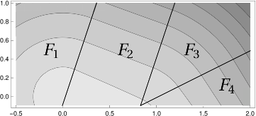
Figure 1: A contour plot of the function $F$.

Proposition 2.1.

1. The function $F$ is convex and 1-smooth over its domain.

2. The function $F$ does not satisfy (2) for $x=(0,0)^{T}$ and $y=(2,0)^{T}$.

Proof.

1. It is straightforward to verify that the quadratic functions $F_{1},\dots,F_{4}$ are convex and 1-smooth. Now, since $F$ is piecewise convex and continuously differentiable it follows that $F$ is convex (see [3, Corollary 5.5]). Finally, the 1-smoothness of $F$ follows from the 1-smoothness of $F_{i}$ by a well-known result on the Lipschitz-continuity of piecewise-continuous functions.

2. We have

   $$F(2,0)=F_{4}(2,0)=\tfrac{16991}{23040}, F^{\prime}(2,0)=F_{4}^{\prime}(2,0)=(\tfrac{253}{240},\tfrac{77}{120})^{T},$$

   $$F(0,0)=F_{1}(0,0)=0, F^{\prime}(0,0)=F_{1}^{\prime}(0,0)=(0,0)^{T},$$

   and therefore

   $$\tfrac{1}{2}\|F^{\prime}(2,0)-F^{\prime}(0,0)\|^{2}=\tfrac{17545}{23040}>\tfrac{16991}{23040}=F(2,0)-F(0,0)-\langle F^{\prime}(0,0),(2,0)^{T}\rangle.$$

∎

As an immediate result of the previous claim, there is no 1-smooth convex function $G:\mathbb{R}^{2}\rightarrow\mathbb{R}$ such that $G(0,0)=F(0,0)$, $G^{\prime}(0,0)=F^{\prime}(0,0)$, $G(2,0)=F(2,0)$ and $G^{\prime}(2,0)=F^{\prime}(2,0)$ (as such an example will form a contradiction to Theorem 1.2). This establishes that the class of smooth and convex functions over an open set is different than the class of unconstrained smooth and convex functions restricted to this set, answering negatively a question raised in [6] of whether all smooth and convex functions defined over an open set can be extended to the entire domain.

3 Properties of convex functions over open sets

In this section we consider the properties of convex functions defined over an open set. We first show that inequality (2) holds for any two points that are close enough. Next, we derive a new analytical bound that holds for any two points in the function’s domain. Finally, we discuss a stronger bound given as a system of inequalities, which can nevertheless be efficiently evaluated numerically.

3.1 A local property

The first main result establishes that locally, a smooth convex function defined over an open set behaves similarly to a smooth and convex function defined over the entire linear space.

Theorem 3.1.

Let $f:C\rightarrow\mathbb{R}$ be an $L$-smooth and convex function over an open convex set $C\subsetneq\mathbb{R}^{d}$. Then for any $x,y\in C$ such that $\|x-y\|<\mathrm{dist}(y,\mathbb{R}^{d}\setminus C)$,

$$\frac{1}{2L}\|f^{\prime}(x)-f^{\prime}(y)\|^{2}\leq f(y)-f(x)-\langle f^{\prime}(x),y-x\rangle.$$

Proof.

The proof is a refinement of the proof in [9, Theorem 2.1.5]. Denote

$$\psi(t):=f(t)-\langle f^{\prime}(x),t-x\rangle,$$

then clearly $\psi$ is $L$-smooth, convex and satisfies $\psi^{\prime}(x)=0$. Furthermore, from the Lipschitz-continuity of $\psi$ we have

$$\|\psi^{\prime}(y)\|=\|\psi^{\prime}(y)-\psi^{\prime}(x)\|\leq L\|y-x\|<L\mathrm{dist}(y,\mathbb{R}^{d}\setminus C),$$

hence $\mathrm{dist}(y,y-\frac{1}{L}\psi^{\prime}(y))<\mathrm{dist}(y,\mathbb{R}^{d}\setminus C)$ which means that $y-\frac{1}{L}\psi^{\prime}(y)\in C$. By applying the Descent Lemma (1) on the points $y$ and $y-\frac{1}{L}\psi^{\prime}(y)$ we have

$$\psi(y-\frac{1}{L}\psi^{\prime}(y))-\psi(y)-\langle\psi^{\prime}(y),y-\frac{1}{L}\psi^{\prime}(y)-y\rangle\leq\frac{L}{2}\|y-(y-\frac{1}{L}\psi^{\prime}(y))\|^{2}$$

or

$$\psi(y-\frac{1}{L}\psi^{\prime}(y))-\psi(y)-\langle\psi^{\prime}(y),-\frac{1}{L}\psi^{\prime}(y)\rangle\leq\frac{L}{2}\|\frac{1}{L}\psi^{\prime}(y)\|^{2}$$

and we get

$$\psi(y-\frac{1}{L}\psi^{\prime}(y))\leq\psi(y)-\frac{1}{2L}\|\psi^{\prime}(y)\|^{2}.$$

Since $x$ is optimal for $\psi$ (recall that $\psi^{\prime}(x)=0$), we have

$$\psi(x)\left(\leq\psi(y-\frac{1}{L}\psi^{\prime}(y))\right)\leq\psi(y)-\frac{1}{2L}\|\psi^{\prime}(y)\|^{2}$$

i.e.,

$$f(x)\leq f(y)-\langle f^{\prime}(x),y-x\rangle-\frac{1}{2L}\|f^{\prime}(x)-f^{\prime}(y)\|^{2}$$

which completes the proof. ∎

An immediate and useful result follows:

Corollary 3.1.

Let $f:C\rightarrow\mathbb{R}$ be an $L$-smooth and convex function over an open convex set $C\subsetneq\mathbb{R}^{d}$ and suppose $x,y\in C$ . Then for any

$$N>\frac{\|y-x\|}{\min(\mathrm{dist}(x,\mathbb{R}^{d}\setminus C),\mathrm{dist}(y,\mathbb{R}^{d}\setminus C))},$$ (3)

the system of inequalities

$$\frac{1}{2L}\|f^{\prime}(x_{i})-f^{\prime}(x_{i+1})\|^{2}\leq f(x_{i})-f(x_{i+1})-\langle f^{\prime}(x_{i+1}),x_{i}-x_{i+1}\rangle, i=0,\dots,N-1,$$ (4)

$$\frac{1}{2L}\|f^{\prime}(x_{i})-f^{\prime}(x_{i+1})\|^{2}\leq f(x_{i+1})-f(x_{i})-\langle f^{\prime}(x_{i}),x_{i+1}-x_{i}\rangle, i=0,\dots,N-1,$$ (5)

holds with

$$x_{i}:=x+\frac{i}{N}(y-x),\quad i=0,\dots,N.$$

Proof.

We have

$$\|x_{i+1}-x_{i}\| =\frac{\|y-x\|}{N}<\min(\mathrm{dist}(x,\mathbb{R}^{d}\setminus C),\mathrm{dist}(y,\mathbb{R}^{d}\setminus C))$$

$$\leq\min(\mathrm{dist}(x_{i},\mathbb{R}^{d}\setminus C),\mathrm{dist}(x_{i+1},\mathbb{R}^{d}\setminus C)),$$

where the last inequality follows since $x_{i}$ are points along the segment $[x,y]$. We conclude that Theorem 3.1 applies for all pairs of points $x_{i}$, $x_{i+1}$, hence (4) and (5) follow. ∎

3.2 A global property

As a consequence of Corollary 3.1, an analytical bound connecting every two points in the set can be established.

Theorem 3.2.

Let $f:C\rightarrow\mathbb{R}$ be an $L$-smooth and convex function over an open convex set $C\subsetneq\mathbb{R}^{d}$. Then for any $x,y\in C$

$$\frac{\langle f^{\prime}(y)-f^{\prime}(x),y-x\rangle^{2}}{2L\|y-x\|^{2}}\leq f(y)-f(x)-\langle f^{\prime}(x),y-x\rangle.$$ (6)

Proof.

For the sake of simplicity we first establish the result for the case where $f$ is 1-smooth and $f^{\prime}(x)=0$.

Let $N$ and $x_{0},\dots,x_{N}$ be defined according to Corollary 3.1, then it follows that inequalities (4) and (5) hold. We start by adding all inequalities in (5) together, obtaining

$$f(y)-f(x)=f(x_{N})-f(x_{0})$$

$$\geq\frac{1}{2}\sum_{i=0}^{N-1}\|f^{\prime}(x_{i})-f^{\prime}(x_{i+1})\|^{2}+\frac{1}{N}\sum_{i=0}^{N-1}\langle f^{\prime}(x_{i}),y-x\rangle$$

$$=\sum_{i=0}^{N-1}\left(\frac{1}{2}\|f^{\prime}(x_{i})-f^{\prime}(x_{i+1})\|^{2}+\frac{i+1}{N}\langle f^{\prime}(x_{i})-f^{\prime}(x_{i+1}),y-x\rangle\right)+\langle f^{\prime}(x_{N}),y-x\rangle.$$

Now, adding (4) and (5) together, we reach

$$\|f^{\prime}(x_{i})-f^{\prime}(x_{i+1})\|^{2}\leq-\frac{1}{N}\langle f^{\prime}(x_{i})-f^{\prime}(x_{i+1}),y-x\rangle, i=0,\dots,N-1.$$ (7)

Let us denote

$$\xi :=N-\frac{\langle f^{\prime}(y),y-x\rangle}{\|y-x\|^{2}}N,$$ (8)

$$\alpha_{i} :=\max\left(0,\xi-i-1,i-\xi\right),\quad i=0,\dots,N-1,$$

then multiplying the inequalities in (7) by $\alpha_{i}$ respectively, we get

$$0 \geq\sum_{i=0}^{N-1}\left(\alpha_{i}\|f^{\prime}(x_{i})-f^{\prime}(x_{i+1})\|^{2}+\frac{\alpha_{i}}{N}\langle f^{\prime}(x_{i})-f^{\prime}(x_{i+1}),y-x\rangle\right).$$

Finally, adding the two last inequalities together and recalling that $f^{\prime}(x_{0})=f(x)=0$ we have

$$f(y)-f(x)$$

$$\geq\sum_{i=0}^{N-1}\left(\frac{2\alpha_{i}+1}{2}\|f^{\prime}(x_{i})-f^{\prime}(x_{i+1})\|^{2}+\frac{\alpha_{i}+i+1}{N}\langle f^{\prime}(x_{i})-f^{\prime}(x_{i+1}),y-x\rangle\right)+\langle f^{\prime}(x_{N}),y-x\rangle$$

$$=\sum_{i=0}^{N-1}\left(\frac{2\alpha_{i}+1}{2}\|f^{\prime}(x_{i})-f^{\prime}(x_{i+1})\|^{2}+\frac{\alpha_{i}-\xi+i+1}{N}\langle f^{\prime}(x_{i})-f^{\prime}(x_{i+1}),y-x\rangle\right)$$

$$\quad+\frac{N-\xi}{N}\langle f^{\prime}(x_{N}),y-x\rangle$$

$$=\sum_{i=0}^{N-1}\left(\frac{2\alpha_{i}+1}{2}\|f^{\prime}(x_{i})-f^{\prime}(x_{i+1})+\frac{\alpha_{i}-\xi+i+1}{N(2\alpha_{i}+1)}(y-x)\|^{2}-\frac{(\alpha_{i}-\xi+i+1)^{2}}{2N^{2}(2\alpha_{i}+1)}\|y-x\|^{2}\right)$$

$$\quad+\frac{N-\xi}{N}\langle f^{\prime}(x_{N}),y-x\rangle$$

$$\geq-\frac{1}{2N^{2}}\sum_{i=0}^{N-1}\frac{(\alpha_{i}-\xi+i+1)^{2}}{2\alpha_{i}+1}\|y-x\|^{2}+\frac{N-\xi}{N}\langle f^{\prime}(x_{N}),y-x\rangle$$

$$=-\frac{\langle f^{\prime}(x_{N}),y-x\rangle^{2}}{2\|y-x\|^{2}}+\frac{\langle f^{\prime}(x_{N}),y-x\rangle^{2}}{\|y-x\|^{2}}=\frac{\langle f^{\prime}(x_{N}),y-x\rangle^{2}}{2\|y-x\|^{2}},$$

where the sum is evaluated in Lemma A.1 in the appendix.

To complete the proof, consider the general case where the assumptions $L=1$ and $f^{\prime}(x)=0$ does not necessarily hold. By setting $\phi(z):=\frac{1}{L}(f(z)-\langle f^{\prime}(x),z-x\rangle)$, we get that $\phi$ satisfies the requirements above and $\phi^{\prime}(z)=\frac{1}{L}(f^{\prime}(z)-f^{\prime}(x))$, hence

$$\frac{\langle\phi^{\prime}(y),y-x\rangle^{2}}{2\|y-x\|^{2}}\leq\phi(y)-\phi(x),$$

which after substitution of the definition of $\phi$ establishes the claim. ∎

As noted above, the bound (6) is strictly stronger than the Descent Lemma (1). Indeed, the lower bound is trivially stronger, and regarding the upper bound, applying Theorem 3.2 with $x$ and $y$ switched then subtracting $\langle f^{\prime}(x),y-x\rangle$ from both sides, we reach

$$f(y)-f(x)-\langle f^{\prime}(x),y-x\rangle\leq\langle f^{\prime}(y)-f^{\prime}(x),y-x\rangle-\frac{\langle f^{\prime}(y)-f^{\prime}(x),y-x\rangle^{2}}{2L\|y-x\|^{2}}$$

$$\leq\langle f^{\prime}(y)-f^{\prime}(x),y-x\rangle\leq\|f^{\prime}(y)-f^{\prime}(x)\|\|y-x\|\leq L\|y-x\|^{2}.$$

A comparison between the bounds is depicted in Figure 2.

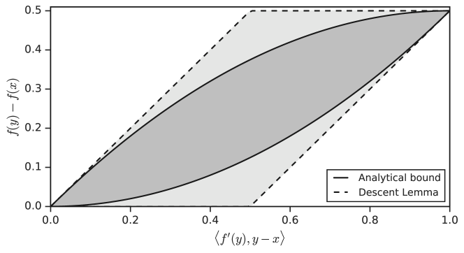
Figure 2: The allowed region for $f(y)-f(x)$ according to the Descent Lemma (outer) and according to Theorem 3.2 (inner) as a function of $\langle f^{\prime}(y),y-x\rangle$, when $L=1$, $f^{\prime}(x)=0$ and $\|y-x\|^{2}=1$.

In the next section we proceed to show that even stronger bounds can be derived from Corollary 3.1, and although we are not aware of an analytical form for these bounds, they can nevertheless be efficiently approximated using standard methods.

3.3 Numerically derived properties

Here we take an alternative look at Corollary 3.1, observing that this system of inequalities can be viewed as a set of constraints on the function values and gradients. These constraints can then be used to form bounds by holding some elements in the inequalities as known and optimizing over the unknown elements.

For example, in order to derive bounds on the value of $f(y)$ given that the values of $x$, $f(x)$, $f^{\prime}(x)$, $y$ and $f^{\prime}(y)$ are known we can take inequalities (4) and (5) as constraints on the value of $f(y)$ treating this value and the values of $f(x_{i})$ and $f^{\prime}(x_{i})$ as unknowns, which we denote by $f_{i}$ and $g_{i}$, respectively. As established by Corollary 3.2 below, an upper bound on the value of $f(y)$ can be obtained by solving the following quadratically-constrained convex optimization problem:

$$U_{N}(x,f_{x},g_{x},y,g_{y}):=\max_{g_{i}\in\mathbb{R}^{d},f_{i}\in\mathbb{R}} \ f_{N}$$

s.t. $$\textstyle\frac{1}{2L}\|g_{i}-g_{i+1}\|^{2}\leq f_{i}-f_{i+1}-\frac{1}{N}\langle g_{i+1},x-y\rangle, 0\leq i<N,$$

$$\textstyle\frac{1}{2L}\|g_{i}-g_{i+1}\|^{2}\leq f_{i+1}-f_{i}-\frac{1}{N}\langle g_{i},y-x\rangle, 0\leq i<N,$$

$$f_{0}=f_{x},\ g_{0}=g_{x},g_{N}=g_{y}.$$

Similarly, a lower bound on $f(y)$ can be established by solving $B_{N}(x,f_{x},g_{x},y,g_{y})$, which is the symmetric problem with a $\min$ operator instead of the $\max$ operator.

Corollary 3.2.

1. Let $f:C\rightarrow\mathbb{R}$ be an $L$-smooth and convex function over an open convex set $C\subsetneq\mathbb{R}^{d}$, and let $x,y\in C$. Then

   $$B_{N}(x,f(x),f^{\prime}(x),y,f^{\prime}(y))\leq f(y)\leq U_{N}(x,f(x),f^{\prime}(x),y,f^{\prime}(y)),$$

   for all values of $N$ satisfying

   $$N>\frac{\|y-x\|}{\min(\mathrm{dist}(x,\mathbb{R}^{d}\setminus C),\mathrm{dist}(y,\mathbb{R}^{d}\setminus C))}.$$

2. Suppose $x,y\in\mathbb{R}^{d}$, $f_{x},f_{y}\in\mathbb{R}$, $g_{x},g_{y}\in\mathbb{R}^{d}$, $L>0$ and $N>0$ are given such that

   $$B_{N}(x,f_{x},g_{x},y,g_{y})\leq f_{y}\leq U_{N}(x,f_{x},g_{x},y,g_{y}).$$

   Then there exists a function $F:\mathbb{R}^{d}\rightarrow\mathbb{R}$ that is $L$-smooth and convex over the segment $[x,y]$, and satisfies

   $$F(x)=f_{x},\ F(y)=f_{y},$$

   $$F^{\prime}(x)=g_{x},\ F^{\prime}(y)=g_{y}.$$

Proof.

1. Let $x_{i}$ be defined as in Corollary 3.1, i.e.,

   $$x_{i}:=x+\frac{i}{N}(y-x),\quad i=0,\dots,N.$$

   Taking

   $$\hat{f}_{i}:=f(x_{i}),\quad i=0,\dots,N,$$

   $$\hat{g}_{i}:=f^{\prime}(x_{i}),\quad i=0,\dots,N,$$

   we get from Corollary 3.1 that $\{\hat{f}_{i}\},\{\hat{g}_{i}\}$ are feasible for $U_{N}(x,f_{x},g_{x},y,g_{y})$. Since the value of the objective at any feasible point is not larger than the optimal solution, we get $f(y)=f(x_{N})=\hat{f}_{N}\leq U_{N}(x,f_{x},g_{x},y,g_{y})$, establishing the upper bound. An identical argument establishes the lower bound.

2. See Appendix B.

∎

Note that the bound introduced in Corollary 3.2 holds for functions that are convex over open sets, however, we have only established that it can be realized by functions that are convex over a line segment. We conjecture that, under the additional assumption that $U_{N}(x,f_{x},g_{x},y,g_{y})$ is strictly feasible, the construction presented in Appendix B can be extended to an open set containing the segment, making the bound in Corollary 3.2 realizable by a smooth convex function over an open set.

Also note that the corollary above demonstrates the approach for the case where $f(y)$ is unknown while all other properties of $f$ at $x,y$ are known, however, by choosing alternative objective and constraints, the same idea can be generalized to allow finding bounds on any combination of the values $x,f(x),f^{\prime}(x),y,f^{\prime}(y)$ with any subset of them being known.

A numerical example

Convex problems of the form $U_{N}$ and $B_{N}$ can be efficiently approximated by interior-point methods [9, 10], allowing the bound in Corollary 3.2 to be numerically evaluated given that all relevant quantities are known.

To illustrate the performance of the bound, consider the case where it is known that $x=0$, $f^{\prime}(x)=0$, $f(x)=0$, $\|y\|^{2}=1$, $\|f^{\prime}(y)\|^{2}=0.5$ and $L=1$; Figure 3 summarizes the allowed range for $f(y)$ obtained from Theorem 3.2 versus the bounds derived by Corollary 3.2 with various values of $N$ and for values of $\langle f^{\prime}(y),y\rangle\in[0.5,\sqrt{0.5}]$ (this corresponds to the interval where problems $U_{N}$ and $B_{N}$ are feasible). As can be seen in the figure, the numerical bound provides a substantial improvement over the analytical one, especially for lower values of $\langle f^{\prime}(y),y\rangle$. We also observe that the value of the bound appears to grow very slowly beyond the first few values of $N$, suggesting that a value of $N$ in the range 5–10 is sufficient for obtaining a highly accurate bound. Finally, note that the range for $N=1$ correspond to the unconstrained bound (2).

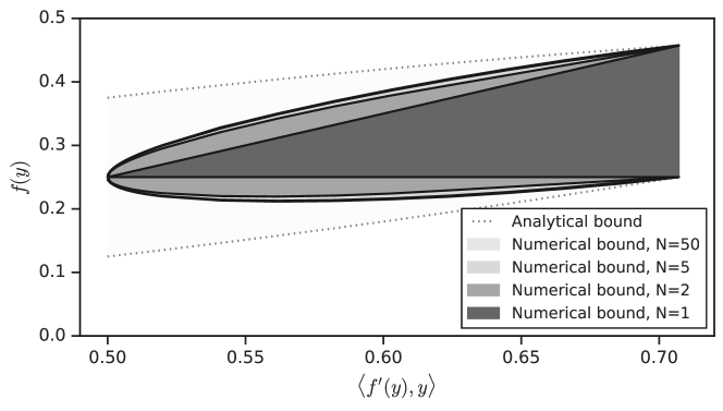
Figure 3: The allowed regions for $f(y)$ according to the analytical bound derived in Theorem 3.2 (dotted lines) and the numerically-derived bounds, plotted as a function of $\langle f^{\prime}(y),y\rangle$, for the case $L=1$, $x=0$, $f^{\prime}(x)=0$, $\|y\|^{2}=1$ and $\|f^{\prime}(y)\|^{2}=0.5$. Note that the regions for $N=5$ and $N=50$ almost completely overlap.

4 Conclusion

We have established some new properties for the class of smooth convex functions over an open set, showing that this class is essentially different than the class of unconstrained smooth convex functions.

These results emphasize the importance of treating this class independently from the class of unconstrained convex functions as is often done in standard texts. In particular, regarding optimization methods, these results suggest that there is benefit in designing specialized methods for each of these two classes of functions, as methods designed for the unconstrained case can make additional assumptions not available in the general case. Moreover, these results show that some care is needed when designing methods for constrained problems, for example, a standard approach for tackling constrained optimization problems is assuming that the problem can be defined by a composite model of the form $F(x)=f(x)+g(x)$, where $f$ is smooth and $g$ is an indicator function that encodes the constraints: this approach, although being natural, limits the applicability of the method to the unconstrained class of functions.

Finally, another interesting question that arises is finding a tight lower complexity bound for the class of constrained functions (in the sense defined by Nemirovsky and Yudin [8]), and whether it differs significantly from the bound in the unconstrained case that was recently established in [7].

Appendix A A technical lemma

Lemma A.1.

Suppose $f:C\rightarrow\mathbb{R}$ is a 1-smooth convex function. Further suppose that $x,y\in C$ and that $f^{\prime}(x)=0$. If $\xi$, $\alpha_{i}$ are defined according to (8), then

$$\sum_{i=0}^{N-1}\frac{(\alpha_{i}-\xi+i+1)^{2}}{2\alpha_{i}+1}=\frac{\langle f^{\prime}(y),y-x\rangle^{2}}{\|y-x\|^{4}}N^{2}.$$

Proof.

First, we observe that

$$\alpha_{i}=\begin{cases}\xi-i-1,&0\leq i<\xi-1,\\ 0,&i\in[\xi-1,\xi],\\ i-\xi,&\xi<i\leq N-1.\end{cases}$$

Now, from the convexity and Lipschitz continuity properties of $f$ we have

$$0\leq\langle f^{\prime}(y),y-x\rangle=\langle f^{\prime}(y)-f^{\prime}(x),y-x\rangle\leq\|y-x\|^{2},$$

which implies $0\leq\xi\leq N$, and thus the set $\{i:\alpha_{i}=0,\ 0\leq i\leq N-1\}$ is not empty. We conclude that there exits some $0\leq N_{1}\leq N$ such that

$$\alpha_{i}=\begin{cases}\xi-i-1,&0\leq i<N_{1},\\ 0,&i=N_{1},\\ i-\xi,&N_{1}<i\leq N-1.\end{cases}$$

We have

$$\sum_{i=0}^{N-1}\frac{(\alpha_{i}-\xi+i+1)^{2}}{2\alpha_{i}+1}$$

$$=\sum_{i=0}^{N_{1}-1}\frac{(\alpha_{i}-\xi+i+1)^{2}}{2\alpha_{i}+1}+(N_{1}-\xi+1)^{2}+\sum_{i=N_{1}+1}^{N-1}\frac{(\alpha_{i}-\xi+i+1)^{2}}{2\alpha_{i}+1}$$

$$=(N_{1}-\xi+1)^{2}+\sum_{i=N_{1}+1}^{N-1}\frac{(2i-2\xi+1)^{2}}{2i-2\xi+1}$$

$$=(N_{1}-\xi+1)^{2}+2\sum_{i=N_{1}+1}^{N-1}i-(N-N_{1}-1)\left(2\xi-1\right)$$

$$=(N_{1}-\xi+1)^{2}+(N-N_{1}-1)(N+N_{1})-(N-N_{1}-1)\left(2\xi-1\right)$$

$$=(\xi-N)^{2}=\frac{\langle f^{\prime}(y),y-x\rangle^{2}}{\|y-x\|^{4}}N^{2}.$$

∎

Appendix B Proof of part 2 in Corollary 3.2

Let $\{\tilde{f}_{i},\tilde{g}_{i}\}$ be an optimal solution for $U_{N}(x,f_{x},g_{x},y,g_{y})$ (this program attains its optimum since its domain is bounded and closed) and set $x_{i}$ as in the first part of the proof. From the constraints in $U_{N}$ it follows that for all $0\leq i\leq N-1$

$$\frac{1}{2L}\|\tilde{g}_{i}-\tilde{g}_{i+1}\|^{2}\leq\tilde{f}_{i}-\tilde{f}_{i+1}-\langle\tilde{g}_{i+1},x_{i}-x_{i+1}\rangle,$$

$$\frac{1}{2L}\|\tilde{g}_{i}-\tilde{g}_{i+1}\|^{2}\leq\tilde{f}_{i+1}-\tilde{f}_{i}-\langle\tilde{g}_{i},x_{i+1}-x_{i}\rangle,$$

hence by the convex extension/interpolation theorems of [1, 14] it follows that there exist $L$-smooth and convex functions $F_{i}:\mathbb{R}^{d}\rightarrow\mathbb{R}$, $i=0,\dots,N-1$, each extending/interpolating the solution between two adjacent points:

$$F_{i}(x_{i})=\tilde{f}_{i},\ F_{i}(x_{i+1})=\tilde{f}_{i+1},\quad i=0,\dots,N-1,$$

$$F^{\prime}_{i}(x_{i})=\tilde{g}_{i},\ F_{i}^{\prime}(x_{i+1})=\tilde{g}_{i+1},\quad i=0,\dots,N-1.$$

Taking $F_{u}$ to be the piecewise function

$$F_{u}(x):=\{F_{i}(x),\ x\in[x_{i},x_{i+1}],\quad i=0,\dots,N-1,$$

it follows from this construction that $F_{u}$ is continuously differentiable and piecewise $L$-smooth and convex hence, as in the proof of Proposition 2.1, $F_{u}$ is $L$-smooth and convex. Furthermore, from the constraints in $U_{N}$ we have

$$F_{u}(x_{0})=F_{0}(x_{0})=\tilde{f}_{0}=f_{x},\ F_{u}^{\prime}(x_{0})=F_{0}^{\prime}(x_{0})=\tilde{g}_{0}=g_{x},$$

$$F_{u}^{\prime}(x_{N})=F_{N-1}^{\prime}(x_{N})=g_{N}=g_{y},$$

and from the optimality of $\{\tilde{f}_{i},\tilde{g}_{i}\}$, we have $F_{u}(x_{N})=\tilde{f}_{N}=U_{N}(x,f_{x},g_{x},y,g_{y})$. Finally, by Whitney’s extension theorem [15], $F_{u}$ can be extended to the entire space $\mathbb{R}^{d}$ while keeping its differentiable structure. Similarly, a function $F_{b}:\mathbb{R}^{d}\rightarrow\mathbb{R}$ that is $L$-smooth and convex over $[x,y]$ can be found such that $F_{b}(x_{0})=\tilde{f}_{0}=f_{x}$, $F_{b}^{\prime}(x_{0})=\tilde{g}_{0}=g_{x}$, $F_{b}^{\prime}(x_{N})=g_{y}$ and $F_{b}(y)=B_{N}(x,f_{x},g_{x},y,g_{y})$. Finally, taking a convex linear combination of the two functions $F_{u}$ and $F_{b}$, we can reach a function $F$ with the claimed properties.

References

- [1] D. Azagra and C. Mudarra. An extension theorem for convex functions of class C1,1 on hilbert spaces. J. Math. Anal. Appl., 446(2):1167–1182, 2017.
- [2] H. H. Bauschke, P. L. Combettes, et al. Convex analysis and monotone operator theory in Hilbert spaces. Springer, 2011.
- [3] H. H. Bauschke, Y. Lucet, and H. M. Phan. On the convexity of piecewise-defined functions. Esaim. Contr. Optim. Ca., 22(3):728–742, 2016.
- [4] A. Beck. First-Order Methods in Optimization. SIAM, 2017.
- [5] A. Daniilidis, M. Haddou, E. Le Gruyer, and O. Ley. Explicit formulas for C1,1 Glaeser-Whitney extensions of 1-Taylor fields in Hilbert spaces. Proc. Am. Math. Soc., 146(10):4487–4495, 2018.
- [6] E. de Klerk, F. Glineur, and A. Taylor. Worst-case convergence analysis of gradient and newton methods through semidefinite programming performance estimation. arXiv preprint arXiv:1709.05191, 2017.
- [7] Y. Drori. The exact information-based complexity of smooth convex minimization. J. Complex., 39:1–16, 2017.
- [8] A. S. Nemirovsky and D. B. Yudin. Problem complexity and method efficiency in optimization. A Wiley-Interscience Publication. John Wiley & Sons Inc., New York, 1983.
- [9] Y. Nesterov. Introductory lectures on convex optimization : a basic course. Applied optimization. Kluwer Academic Publ., 2004.
- [10] Y. Nesterov and A. Nemirovskii. Interior-point polynomial algorithms in convex programming, volume 13. Siam, 1994.
- [11] J. M. Ortega and W. C. Rheinboldt. Iterative solution of nonlinear equations in several variables, volume 30. Siam, 1970.
- [12] B. T. Polyak. Introduction to Optimization. Translations Series in Mathematics and Engineering. Optimization Software, 1987.
- [13] R. T. Rockafellar. Convex analysis. Princeton university press, 2015.
- [14] A. B. Taylor, J. M. Hendrickx, and F. Glineur. Smooth strongly convex interpolation and exact worst-case performance of first-order methods. Math. Program., 161(1-2):307–345, 2017.
- [15] H. Whitney. Analytic extensions of differentiable functions defined in closed sets. Trans. Am. Math. Soc., 36(1):63–89, 1934.