Self-supervised Learning of Dense Shape Correspondence
Abstract
We introduce the first completely unsupervised correspondence learning approach for deformable 3D shapes. Key to our model is the understanding that natural deformations (such as changes in pose) approximately preserve the metric structure of the surface, yielding a natural criterion to drive the learning process toward distortion-minimizing predictions. On this basis, we overcome the need for annotated data and replace it by a purely geometric criterion. The resulting learning model is class-agnostic, and is able to leverage any type of deformable geometric data for the training phase. In contrast to existing supervised approaches which specialize on the class seen at training time, we demonstrate stronger generalization as well as applicability to a variety of challenging settings. We showcase our method on a wide selection of correspondence benchmarks, where we outperform other methods in terms of accuracy, generalization, and efficiency.
1 Introduction
The problem of finding accurate dense correspondence between non-rigid shapes is fundamental in geometry processing. It is a key component in applications such as deformation modeling, cross-shape texture mapping, pose and animation transfer to name just a few. Dense deformable shape correspondence algorithms can be broadly categorized into two families. The first can be referred to as axiomatic or model-based: A certain geometric assumption is asserted and pursuit for by some numerical scheme. Modeling assumptions attempt to characterize the action of a class of deformation on some geometric quantities commonly referred to as descriptors. Such geometric quantities often encode local geometric information in the vicinity of a point on the shape (point-wise descriptors) such as normal orientation [43], curvature [34], and heat [41] or wave [6] propagation properties. Another type of geometric quantities are the global relations between pairs of points (pair-wise descriptors), which include geodesic [18, 12], diffusion [15] or commute time [46] distances. Given a pair of shapes, a dense map between them is sought to minimize the discrepancy between such descriptors. While the minimization of the point-wise discrepancies can be formulated as a linear assignment problem (LAP) and solved efficiently for reasonable scales, the use of pair-wise descriptors leads to a quadratic assignment problem (QAP) that is unsolvable for any practical scales. Numerous approximations and heuristics have been developed in the literature to alleviate the computational demand of QAPs.
The second family of correspondence algorithms is data-driven and takes advantage of modern efficient machine learning tools. Instead of axiomatically modeling the class of deformations and the geometric properties of the shapes of interest, these methods infer such properties from the data themselves. Among such approaches are learnable generalizations of the heat kernel signature [29], as well as works interpreting correspondence as a labeling problem [37]. Other recent methods generalize CNNs to non-Euclidean structures for learning improved descriptors [32, 10]. A recent method based on extrinsic deformation of a null-shape was introduced in [20]. A common denominator of these approaches is the supervised training regime – they all rely on examples of ground truth correspondences between exemplar shapes.
A major drawback of this supervised setting is the fact that in the case of 3D shape correspondence the ground truth data are scarce and very expensive to obtain. For example, despite being restricted to a single shape class (human bodies), the MPI FAUST scanning and labeling system [8] required substantial manual labor and considerable financial costs. In practice, labeled models are expected to be just a small fraction of the existing geometric data, bringing into question the scalability of any supervised learning algorithm.
1.1 Contribution
We propose an unsupervised learning scheme for dense 3D deformable shape correspondence based on a purely geometric criterion. The suggested approach bridges between the model-based and the data-driven worlds by learning point-wise descriptors that result in correspondences minimizing pair-wise geodesic distance disagreement. The correspondence is then solved for using the functional maps framework [33] totally avoiding the computational burden of the pair-wise methods. While the point-wise descriptors are learned on a surrogate task only approximately characterizing the real data (which deviate from the asserted isometric deformation model), the method shows excellent generalization capabilities exceeding the supervised counterparts without ever seeing examples of ground truth correspondences. To the best of our knowledge, this is the first unsupervised approach applied to the geometric problem of finding shape correspondence.
A major advantage of the proposed framework is when the data themselves are scarce, in extreme conditions we might have only one pair of shapes that we would like to match and we do not have a training dataset that contains similar shapes. While a supervised scheme depends on a relatively large amount of labelled data to deduce a generalizing model, with the unsupervised network we can simply optimize on a single pair of shapes that by itself contains two training samples, one in each direction of the correspondence. Our experiments required only a few iterations that take just a couple of minutes to run. Usually, less than iterations were more than enough. As a result we obtain an accurate matching between the shapes, see Figure 1. For a trained network the inference phase takes less than a second. We believe that this strategy has its own merits as a replacement of the existing computationally expensive methods that are based on pair-wise descriptors. The framework can be interpreted as a fusion between the previously proposed FMNet, the Functional Maps centered network architecture [26] and the pair-wise geodesic distance distortion criterion used in previously proposed model-based approaches such as GMDS [12].
2 Background
2.1 Minimum distortion correspondence
We model shapes as Riemannian 2-manifolds equipped with a distance function induced by the standard volume form. An isometry is a map satisfying, for any pair :
| (1) |
Correspondence seeking approaches optimize for a map satisfying the distance preservation criterion (1). In practical applications, only approximate realizations of an isometry are expected; thus, one is interested in identifying a distortion-minimizing map of the form
| (2) |
In the discrete setting, we assume manifolds to be represented as triangle meshes sampled at vertices each. Minimum distortion correspondence thus takes the form of a quadratic assignment problem (QAP), where the minimum is sought over the space of permutation matrices.
Several studies have tried to reduce the complexity of this QAP at the cost of getting an approximate solution via sub-sampling [42, 35], hierarchical matching [12, 47] or convex relaxations [3, 14].
However, complicated to solve, the minimum distortion criterion (2) is axiomatic and does not require any annotated correspondences, making it a natural candidate for an unsupervised learning loss.
2.2 Descriptor learning
A common way to make the optimization of (2) more efficient is by restricting the feasible set to include only potential matches among points with similar descriptors. By doing so, one shifts the key difficulty from optimizing a highly non-linear objective to designing deformation-invariant local point descriptors.
This has been an active research goal in shape analysis in the last few years, with examples including GPS [38], heat and wave kernel signatures [41, 6], and the more recent geodesic distance descriptors [40]. In 3D vision, several rotation-invariant geometric descriptors have been proposed [43, 23]. Despite their lack of invariance to isometric deformations, however, the adoption of extrinsic descriptors has been advocated in deformable settings [36] due to their locality and resilience to boundary effects. Handcrafted descriptors suffer from an inherent drawback of requiring manual tuning. Learning techniques have thus been proposed to define descriptors whose invariance classes are learned from the data. Early examples include approaches based on decision forests and metric learning [29, 37, 17]; more recently, several papers have proposed an adaptation of deep learning models to non-Euclidean domains, achieving dramatic improvement. In [31, 10, 32] learnable local filters were introduced based on the notion of patch operator.
In [26] a task driven approach was taken instead, where the network learns descriptors which excel at the task at hand in a supervised manner (this will be discussed in detail in Section 2.4). As we will show in the sequel, our approach builds upon this model while completely removing the need for supervision.
2.3 Functional maps
The notion of functional map was introduced in [33] as a tool for transferring functions between surfaces without the direct manipulation of a point-to-point correspondence. Let be real-valued functional spaces defined on top of and respectively. Then, given a bijection , the functional map is a linear mapping acting as
| (3) |
The functional map admits a matrix representation with respect to orthogonal bases on and respectively, with coefficients calculated as follows:
| (4) |
While the functional maps formalism makes no further requirements on the chosen bases, a typical choice is the Laplace-Beltrami eigenbasis (the justification for the optimality of this choice can be found in [2]).
Truncating these series to coefficients, one obtains a band-limited approximation of the functional correspondence . Specifically, the map
| (5) |
also referred to as a soft map, will assign to each point a function concentrated around with some spread.
To solve for the matrix , linear constrains are derived from the knowledge of knowingly corresponding functions on the two surfaces. Corresponding functions are functions that preserve their value under the mapping . Given a pair of corresponding functions and with coefficients and in the bases and respectively, the correspondence imposes the following linear constraint on
| (6) |
Each pair of such corresponding functions is translated into a linear constraint.
Suppose there exists an operator receiving a shape and producing a set of descriptor functions on it. Let us further assume that given another shape , the operator will produce a set of corresponding functions related by the latent correspondence between and . In other words, applying the above operator on the said pair of shapes produces a set of pairs of corresponding functions , each pair comprising defined on and on . We stack the corresponding coefficients and into the columns of the matrices and . The functional map matrix is then given by the (least squares, or otherwise regularized) solution to the system
| (7) |
Thus, the requirement for specific knowledge of the point-to-point correspondence is replaced by the relaxed requirement of knowledge about functional correspondence.
2.4 Deep functional maps
A significant caveat in the above setting is that, unless the shapes and are related by a narrow class of deformations, it is very difficult to construct an operator producing a sufficient quantity of stable and repeatable descriptors. However, such an operator can be learned from examples. The aim of the deep functional maps network (FMNet) introduced in [26] was to learn descriptors which, when used in the above system of equations, will induce an accurate correspondence. At training time, FMNet operates on input descriptor functions (e.g. SHOT descriptors), and improves upon them by minimizing a geometric loss that is defined on the soft correspondence derived from the functional map matrix. The differentiable functional map layer (FM), solves the equation (7), with the current descriptor functions in each iteration.
The network architecture described in [26] consists of fully-connected residual layers with exponential linear units (ELU) and no dimentionality reduction. The output of the residual network is a dense vector-valued descriptor. Given two shapes and , the descriptors are calculated on each shape using the same network, and are projected onto the corresponding truncated LBO bases. The resulting coefficients are given as an input to the functional map (FM) layer that calculates the functional map matrix according to (7). The following correspondence layer (Corr) produces a soft correspondence matrix out of the functional map matrix ,
| (8) |
Where we denoted the number of vertices on the discretized shapes as and , and the diagonal matrix normalizes the inner products with the discrete area elements of . The absolute value and the column normalization, denoted by ∥⋅∥, ensure that the values of can be interpreted as the probability of vertex on shape being in correspondence with vertex on . We denote the element-wise square of by , with standing for the Hadamard product.
Treating the -th column of , , as the distribution on the points of corresponding to the point on , we can evaluate the expected deviation from the ground truth correspondence . This is expressed by the second-order moment
| (9) |
where is the geodesic distance on between the vertex and the ground truth match of the vertex on . As usual, this moment comprises a variance and a bias terms; while the former is the result of the band-limited approximation (due to the truncation of the basis), the latter can be controlled.
Averaging the above moment over all points on leads to the following supervised loss
| (10) | |||||
where denotes the pairwise geodesic distance matrix evaluated for each shape at the pre-processing stage, and is the ground truth permutation relating between the shapes. The batch loss is the sum of for all the pairs in the minibatch.
Training an FMNet follows the standard Siamese setting commonly used for descriptor or metric learning, in which two copies of the network with shared parameters produces the descriptors on and . From this perspective, the functional map and the soft correspondence layers are parts of the Siamese loss rather than of the network itself.
3 Unsupervised deep functional maps
The authors in [26] showed that FMNet achieves state-of-the-art performance on standard deformable shape correspondence benchmarks. However, one can argue that the supervised training regime is prohibitive in terms of the amounts of the manually annotated data required.
The main contribution of this paper is the transition to an unsupervised training regime, i.e., a setting requiring no ground-truth correspondence. The key idea is that even if ground truth correspondence is not provided, we can still evaluate the quality of the resulting correspondence based on the preservation of standard geometric quantities. As mentioned before, human pose articulation can be modeled as approximate isometries, that is, the latent correspondence introduces little metric distortion. If two vertices were at some geodesic distance on the source shape, after mapping by the correct correspondence, the distance between corresponding points on the target domain is preserved.
Let be the output of the soft correspondence layer of an FMNet; as before, its squared elements are interpreted as probability distributions on . In these terms, the -th element of the matrix
| (11) |
represents the expected distance on between the images of the vertices under the soft correspondence .
This allows to define the following unsupervised loss
| (12) |
The batch loss is the sum of for all the pairs in the minibatch. This loss measures the geodesic distance distortion and can be interpreted as a soft correspondence version of the GMDS loss, see [4]. Note that rather than solving the QAP directly, we propose to train an FMNet using , which promotes the network to generate descriptors for which the resulting soft correspondence minimizes the expected pairwise distance distortion.
From the point of view of the unsupervised network all the shapes in the world could constitute a training set. Since the network does not use any ground-truth correspondence data, its learning is not limited to a class of shapes and is expected to improve when new shapes are encountered. The strict separation between the training and test sets that characterizes the supervised regime does not strictly apply in the unsupervised setting, since the network does not make any distinction between training and testing shapes. If the training set is representative enough to generalize the test set, the network can learn on the training set and infer on the test set, reducing the processing time per shape. Contrarily, if the training set is not representative enough, the network can still gain advantage from being exposed to the test shapes and using them to improve the learned model. Learning could in fact be executed even at inference time. For the FAUST scans [7], for example, the authors provide a training test with ground-truth labeling and a disjoint test set without the labels. A supervised scheme cannot gain much from seeing the test shapes since they lack the ground truth correspondence, and it is confined to train on the training set alone. The unsupervised scheme has access to the same data, but contrarily to the supervised counterpart, it can use the unlabeled test shapes to improve prediction accuracy.
4 Implementation
We implemented our network in TensorFlow [1], running on a GeForce GTX 1080 Ti GPU. Data preprocessing and correspondence refinement were done in Matlab.
4.1 Pre-processing
To enable mini-batches of multiple shapes to fit in memory, each shape in the training set was remeshed to between K and K vertices , by edge contraction [19]. For each remeshed shape Laplace-Beltrami eigenfunctions were calculated as well as a -dimensional SHOT descriptor [39], using 10 bins and a SHOT radius that was roughly chosen to 5% of the maximal pairwise geodesic distance. Geodesic distance matrices were estimated using the fast marching method [25]. These quantities constitute the input to the network.
4.2 Network architecture and loss
For a more direct and fair comparison, we adopted the same network architecture as FMNet presented in Figure 2. Specifically, the input for each pair of shapes is their truncated LBO bases and , the pairwise distance matrices and , and the SHOT descriptor fields . These are fed to a -layer residual network [21] outputting -dimensional dense descriptor fields and on and respectively, which can be thought of as non-linearly transformed variants of SHOT.
The computed descriptors are then input to the functional map layer, yielding a functional map matrix according to (7), followed by a soft correspondence layer producing the stochastic correspondence matrix as per Eq. (8). Finally, the unsupervised loss is calculated according to Eq. (12). While in FMNet the loss is calculated on a random sub-sampling of the vertices, we found that this strategy introduces inaccuracies to the descriptor coefficients in the LBO basis. When sub-sampling is used, the network is only able to evaluate an estimate of the projection of the descriptors onto the LBO basis, which quickly becomes inaccurate for descriptors with high-frequency content. To avoid this, in our implementation we perform the projection at full resolution while decreasing the size of the mini-batch to 4–5 pairs of shapes per mini-batch. In all our experiments we used no more than a few thousands (about 3K–10K) mini-batch iterations. For comparison, the supervised FMNet used 100K iterations of mini-batch size to achieve similar results.
4.3 Post-processing
Point-wise map recovery. Following the protocol of FMNet, we apply the product manifold filter (PMF) [45] to improve the raw prediction of the network. This algorithm takes noisy matches as input, and produces a (guaranteed) bijective and smoother correspondence of higher accuracy as output. The application of PMF boils down to solving a series of linear assignment problems , where ranges over the space of permutations, and are kernel matrices acting as a diffusion operators. We refer to [45] for additional details.
Upscaling. Since we operate on remeshed shapes, we finally apply an upscaling step to bring the correspondence back to the original resolution. Again, we follow the procedure described in FMNet [26], namely we solve a functional map estimation problem of the form
| (13) |
where contain the LBO coefficients (in the full resolution basis) of delta functions supported at corresponding points, extracted from the low resolution map . The norm (defined as the sum of norms of the columns) allows to downweight potential mismatches.
5 Experiments
5.1 Learning to match a single pair
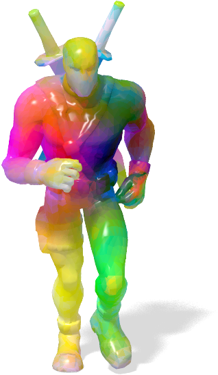
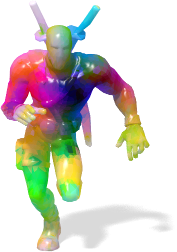
Before delving into training on large datasets, we begin our experimental section with testing one extreme of the shape matching problem: single input pair. Clearly, this is the native environment for classical, non-learning based methods. While learning based methods have endowed us with better solutions given large train sets, they are not equipped to handle entirely novel examples. Having developed an unsupervised network we demonstrate it can be utilized as an ad-hoc solver for a single pair, producing excellent results. In Figure 1 we show our result on a pair of shapes made by an artist111credit to the artist appears in the Acknowledgements section. Note that we do not have groundtruth correspondences for this pair and therefore a supervised learning based method cannot be fine-tuned on the input pair. Instead we compare with raw predictions of FMNet that has been pre-trained on human shapes from FAUST. In addition, we ran the post processing procedure described in 4.3. While we got comparable results to our method (please see Appendix A for visualization), runtime has exceeded one hour. Conversely, optimizing our network took about minutes. Furthermore, had we been given an additional deformation of the same shape to solve for, an axiom-based method would have needed to solve the problem from scratch. Differently, as our method had already learned to convert the pair-wise optimization problem to a descriptor matching problem, inference would take about one second!
5.2 Faust synthetic
Faust synthetic models [7] are a widely used data in shape matching tasks. In this experiment we use it for comparing our unsupervised method and its supervised counterpart under the same setting. We show that (a) optimizing for the unsupervised loss results in a correlated decrease of the supervised loss; (b) the unsupervised method, achieves the same accuracy as the supervised one. For training our network, We followed the same dataset splits as in [26] where the first shapes of subjects are used for training, while a disjoint set of shapes of other subjects were used for testing. Each training mini-batch contained pairs of shapes in their full resolution of vertices. Since the corresponding vertices in the dataset have corresponding indices, we shuffled randomly the vertices of each shape in the training pair, for every new appearance in the training mini-batches, creating a nontrivial permutation between the corresponding vertices. This step is intended to eliminate the possibility that the network converges to descriptors that lead always to the trivial permutation. We used the same parameters as in [26], namely, eigenfunctions and ADAM optimizer with a learning rate of and . We used training mini-batches. Note that, as in [26], since we train on pairs of shapes we have an effective train set size of .
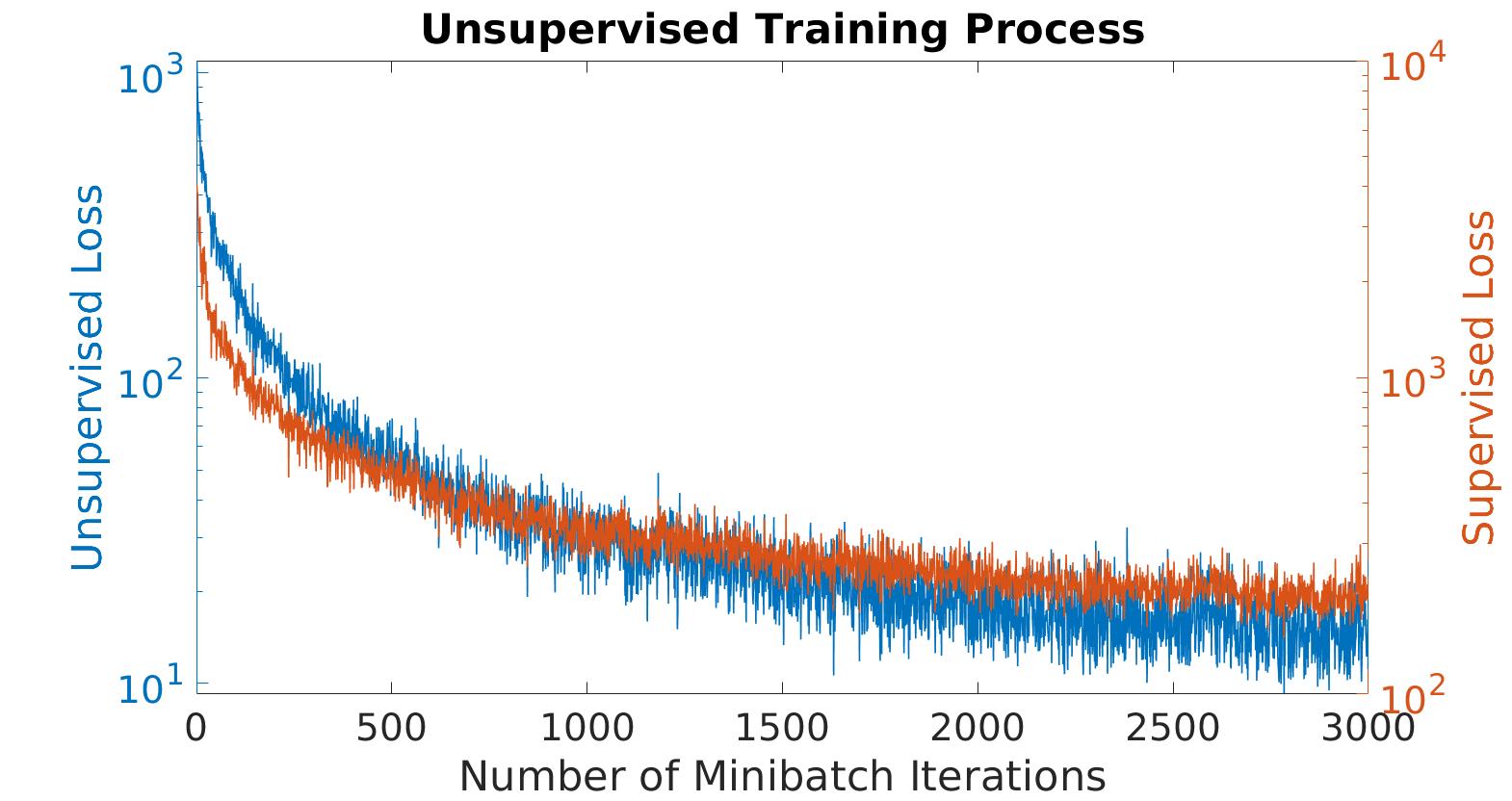
Loss function analysis. Figure 3 displays the unsupervised loss during the training process (top), alongside with the supervised loss (bottom). Importantly, the unsupervised network had no access to ground truth correspondence.
From the graphs, it can be observed that while the optimization target is the unsupervised loss, the supervised loss is decreased as well. This demonstrates nicely that when our underlying assumption of (quasi-) isometric deformations holds, one can replace the expensive supervision altogether with a single axiomatic-driven loss term.
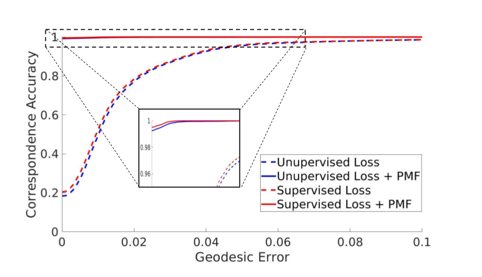
Performance comparison. To compare our results with the supervised network, we followed the same training scheme, this time using the supervised loss. We used the test shapes to construct a test dataset of pairs in total; of which are of the same subject at different poses, and the other are of different subjects at different poses (Note that the matching is directional from source to target, hence this set is not redundant). The intra-subject pairs, are well modeled by isometry while the inter-subject pairs exhibit deviation from isometry. For each test pairs the vertices of both shapes were shuffled separately in a random manner (but consistent between the two networks). Figure 4 compares the results for the intra-subject pairs in synthetic Faust. Figure 5 visualizes the calculated correspondences.
5.3 Real scans
Traditionally, axiom-based methods were proven useful only in the Computer Graphics regime. One of our goals in introducing learned descriptors is to demonstrate the applicability of our method to real scanned data. To this end, we make use of FAUST real scans benchmark. These are very high-resolution, non-watertight meshes, many of which contain holes and topological noise. We used the dataset split as prescribed in the benchmark. The scans were down-sampled to a resolution of K vertices. For each scan the distance matrix was calculated, as well as -dimensional SHOT descriptors and LBO eigenfunctions. Each training mini-batch contained pairs of shapes. We trained our network for iterations. The raw network predictions were only upscaled but not refined with PMF. Quantitative results were evaluated through the online evaluation system. With an average and worst case scores of cm and cm, respectively, on the intra challenge, our network performs on par with state of the art methods that do not use additional data; namely, FMNet (, ), and Chen et al. [14] (, ). We perform slightly below the recent 3D-CODED method [20] (, ) which uses an additional augmentation of over K shapes at training. The same method, when not using additional data achieves worse results by a factor of .
5.4 Generalization
Having an unsupervised loss grants us the ability to train on datasets without given dense correspondences, or even to optimize on individual pairs. Both methods were demonstrated in the previous experiments. In this subsection, however, we would like to pose a different question: what has our network learned by training on a source dataset, and to which extent this knowledge is transferable to a target one. Transferability between training domains is a long-standing research area that has recently re-gained lots of interest, yet it hasen’t been explored as much in the shape analysis community. In the scope of this work we focus on transferring from either the synthetic or scanned FAUST shapes to the either (a) human shapes form Dynamic-FAUST, (b) human shapes form SCAPE, and (c) Animal shapes from TOSCA.
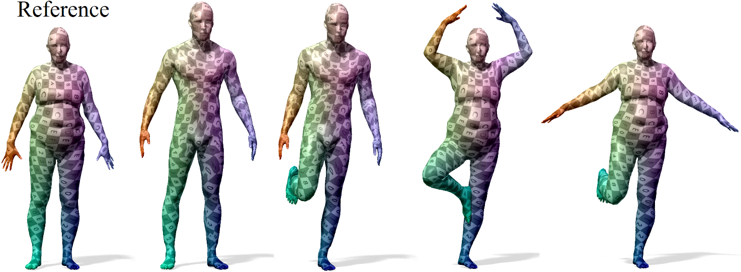
Dynamic FAUST is a recent very large collection of human shapes [8], demonstrating various sequences of activities. While the shapes are triangulated in the same way as our train set of synthetic FAUST, they significantly differ in pose and appearance. Figure 8 shows excellent generalization to this set, suggesting that the small set of synthetic FAUST shapes were sufficient to capture the pose and shape variability. Please see Appendix B for more visualizations.
SCAPE dataset [5] also comprises human shapes only. Yet, we’ve witnessed a quite poor performance using the network trained on synthetic data. By the same reasoning behind the former result, the network might have learned to specialize on the synthetic connectivity. To circumvent this, we have tested the network trained on scans, that demonstrate different meshes. Indeed it can be seen that the generalization improved significantly.
TOSCA dataset [13] includes various animal shapes. Interestingly, the network trained on scans showed very good performance without ever seeing a single animal shape at train time. In Figure 6 we compare the results with a network trained separately on each animal category and show comparable results before pre-processing, and near-perfect results after.
5.5 Partial correspondence
Partial shape correspondence is a notoriously hard problem, and techniques that aim at solving it often require special care [27, 36, 28]. That said, in this experiment we tested the performance of our method under extreme partiality conditions as is, namely, without any modification to our network. To this end, we used the challenging “dog with holse” class from [16]. We trained the network on a small set of partial shapes, and evaluated the results test shapes. The network results are shown in Figure 7.
We found that the mismatches occur typically near the boundary of the partial shape. The reason might be the distortion of the SHOT descriptor in these regions.
6 Discussion and conclusions
The main message of the paper is that a properly designed unsupervised surrogate task can replace massive labeling. While we advocate the pure unsupervised approach as a replacement to the supervised one, the two can also be combined in a semi-supervised learning scheme. While we demonstrate that the minimization of geodesic distance distortion achieves good generalization on a variety of benchmarks, local scale variation and topological changes can challenge the classic model and require a proper adaptation. In future studies, we intend to investigate training tasks based on the preservation of more general scale- and conformal-invariant pair-wise geometric quantities, as well as topological properties, e.g. by utilizing pairwise diffusion distances. The proposed network exhibits surprisingly high performance on partial correspondence tasks, even though the functional map layer is not explicitly designed to treat partial data. Extending it to the partial setting based, e.g., on the recently introduced partial functional map formalism [36, 27] will be the subject of further investigation. Finally, we would like to explore additional descriptor fields with enhanced properties like increased sensitivity to symmetries, increased robustness to partiality and non rigid deformations. Our work is a first attempt to create a fully unsupervised learning framework to solve the fundamental problem of non rigid shape correspondence. We believe that the fusion of axiomatic models and deep learning is a promising direction that makes it possible to accommodate the expected future growth of 3D data.
Acknowledgements
This research was partially supported by the Israel Ministry of Science, grant number 3-14719 and the Technion Hiroshi Fujiwara Cyber Security Research Center and the Israel Cyber Bureau. Alex Bronstein was supported by ERC grant no. 335491 (RAPID). Emanuele Rodolà was supported by ERC grant no. 802554 (SPECGEO).
Appendix A Training with scarce data
As discussed in Section 5.1, having an unsupervised learning method bridges the gap between axiomatic solvers and supervised learning methods. The latter can excel on particular data but often suffer from limited generalization capabilities, while the former offer a general purpose tool for solving matches between unseen pairs but suffer from computational inefficiency. Our method can do both, while demonstrating improved capabilities in both regimes. The TOSCA experiment in Section 5.4 (Figure 6) shows that our network trained on human scans generalizes well to non-human shapes. The single-pair experiment in Section 5.1 (Figure 1) shows that our method can efficiently solve for a single unseen pair of shapes. In addition, we have emphasized its usefulness in fast inference given a scarce unlabeled train set. In what follows we present additional evidence that did not fit into the main paper due to page limitation.
Learning to match a single pair. The extreme, one-pair settings described in Section 5.1 of the main manuscript, compared our method and a supervised learning-based one. Here Figure 10 provides an additional comparison with an axiomatic method: Functional Maps [33] with SHOT descriptors [43], refined with PMF [44]. Interestingly, this computationally intensive method is still inferior to ours.
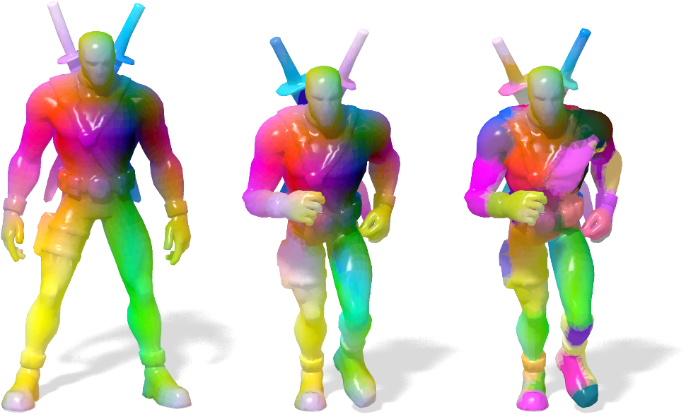
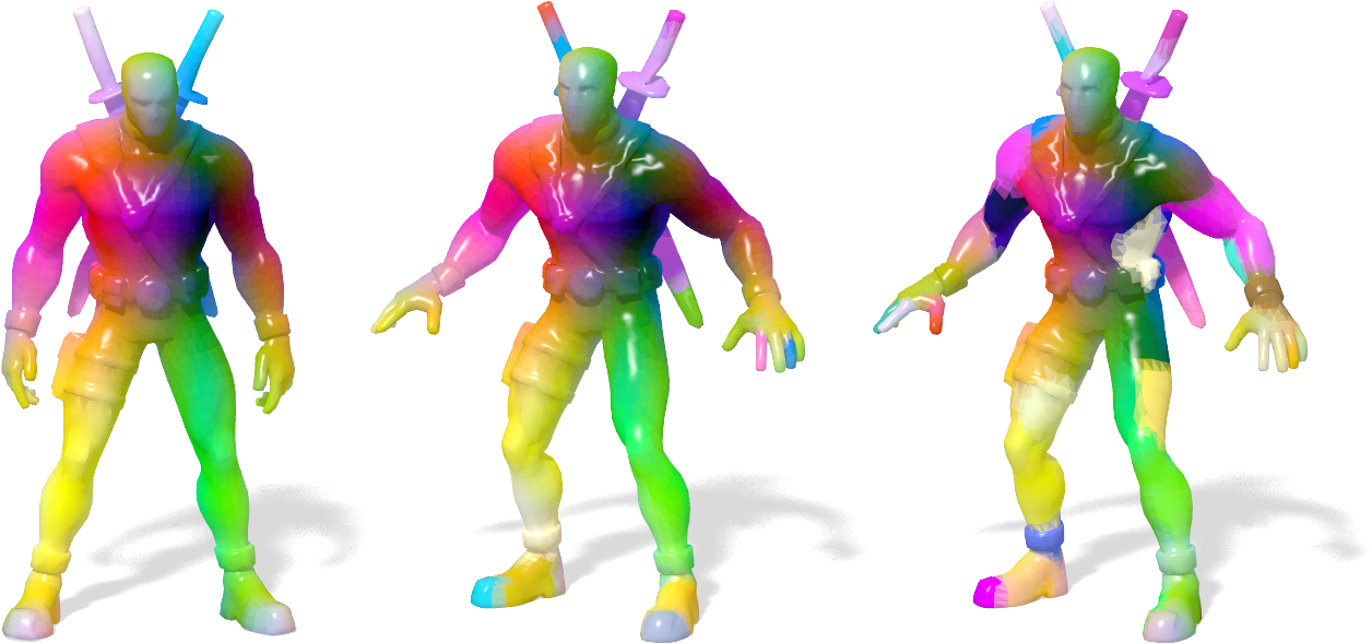
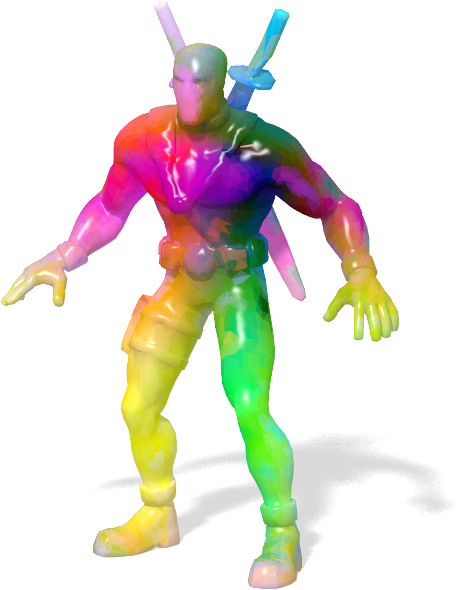
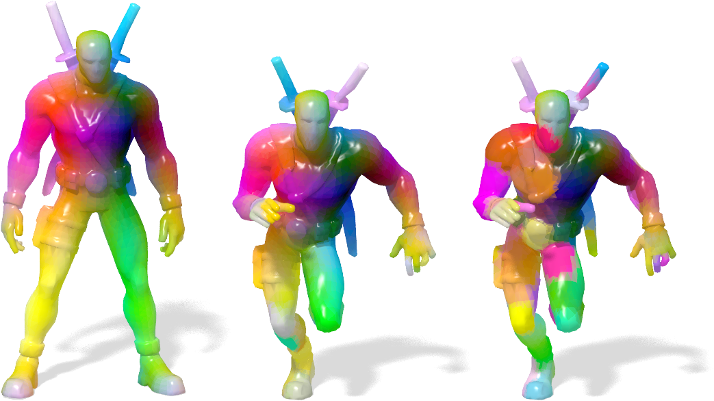
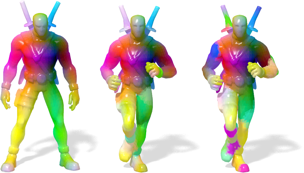
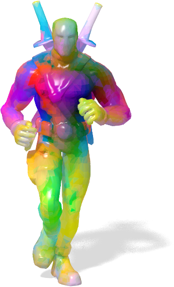
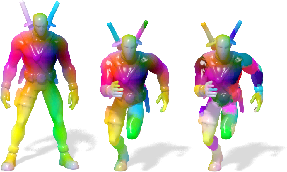
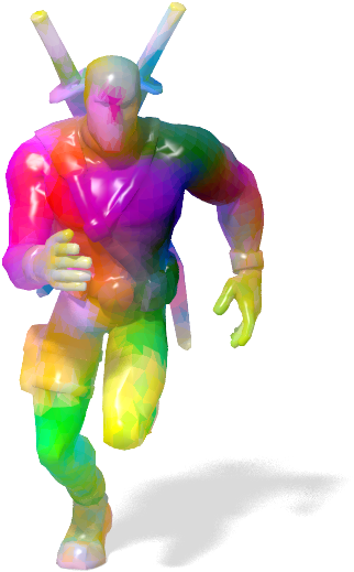
Fast inference. As discussed above, when fast inference is required on newly encountered unlabeled data, axiomatic methods are no longer an option. Also, one cannot afford full retraining and therefore has two options: either using a pre-trained network on a labelled similar data using supervised learning, or use the unsupervised network to train quickly on few examples. We demonstrate this using an artistic model of Deadpool, a super-hero comics character, provided in a variety of poses sampled from animations.
To convert the artistic mesh to a manifold we used [22]. The models were remeshed to a K resolution, using edge contraction [19]. We wish to stress that the artistic models do not have any ground-truth labeling, emphasizing the usefulness of an unsupervised approach.
In Figure 11 we compare the performance of the unsupervised network, trained with only shapes for a total of minutes ( iterations); and the supervised network trained on FAUST synthetic human dataset ( shapes) for hours (K iterations). Visualized are the test examples (i.e., pairs of shapes unavailable to the network at training time). While both methods demonstrate equivalent inference time of less than one second, the performance gap is significant showing a clear advantage for our method.
Appendix B MPI Dynamic FAUST additional visualization
Section 5.4 discusses the generalization of our network, trained on the FAUST synthetic human dataset, on the recent Dynamic FAUST dataset [8]. As demonstrated in Figure , when tested on test pairs comprising different subjects at different poses, our method showed extremely good results. To save space, we only included few visualizations. In Figure 12 we show many more results via texture transfer.
References
- [1] M. Abadi, A. Agarwal, P. Barham, E. Brevdo, Z. Chen, C. Citro, G. S. Corrado, A. Davis, J. Dean, M. Devin, S. Ghemawat, I. Goodfellow, A. Harp, G. Irving, M. Isard, Y. Jia, R. Jozefowicz, L. Kaiser, M. Kudlur, J. Levenberg, D. Mané, R. Monga, S. Moore, D. Murray, C. Olah, M. Schuster, J. Shlens, B. Steiner, I. Sutskever, K. Talwar, P. Tucker, V. Vanhoucke, V. Vasudevan, F. Viégas, O. Vinyals, P. Warden, M. Wattenberg, M. Wicke, Y. Yu, and X. Zheng. TensorFlow: Large-scale machine learning on heterogeneous systems, 2015. Software available from tensorflow.org.
- [2] Y. Aflalo, H. Brezis, and R. Kimmel. On the optimality of shape and data representation in the spectral domain. SIAM Journal on Imaging Sciences, 8(2):1141–1160, 2015.
- [3] Y. Aflalo, A. Bronstein, and R. Kimmel. On convex relaxation of graph isomorphism. Proceedings of the National Academy of Sciences, 112(10):2942–2947, 2015.
- [4] Y. Aflalo, A. Dubrovina, and R. Kimmel. Spectral generalized multi-dimensional scaling. IJCV, 118(3):380–392, 2016.
- [5] D. Anguelov, P. Srinivasan, D. Koller, S. Thrun, J. Rodgers, and J. Davis. SCAPE: Shape Completion and Animation of People. TOG, 24(3):408–416, 2005.
- [6] M. Aubry, U. Schlickewei, and D. Cremers. The wave kernel signature: A quantum mechanical approach to shape analysis. In Proc. ICCV Workshops, pages 1626–1633, 2011.
- [7] F. Bogo, J. Romero, M. Loper, and M. J. Black. FAUST: Dataset and Evaluation for 3d Mesh Registration. In Proc. CVPR, 2014.
- [8] F. Bogo, J. Romero, G. Pons-Moll, and M. J. Black. Dynamic FAUST: Registering human bodies in motion. In IEEE Conf. on Computer Vision and Pattern Recognition (CVPR), July 2017.
- [9] D. Boscaini, J. Masci, S. Melzi, M. M. Bronstein, U. Castellani, and P. Vandergheynst. Learning class-specific descriptors for deformable shapes using localized spectral convolutional networks. Computer Graphics Forum, 34(5):13–23, 2015.
- [10] D. Boscaini, J. Masci, E. Rodolà, and M. Bronstein. Learning shape correspondence with anisotropic convolutional neural networks. In Advances in Neural Information Processing Systems, pages 3189–3197, 2016.
- [11] D. Boscaini, J. Masci, E. Rodolà, M. M. Bronstein, and D. Cremers. Anisotropic diffusion descriptors. In Computer Graphics Forum, volume 35, pages 431–441. Wiley Online Library, 2016.
- [12] A. M. Bronstein, M. M. Bronstein, and R. Kimmel. Generalized multidimensional scaling: a framework for isometry-invariant partial surface matching. PNAS, 103(5):1168–1172, 2006.
- [13] A. M. Bronstein, M. M. Bronstein, and R. Kimmel. Numerical geometry of non-rigid shapes. Springer Science & Business Media, 2008.
- [14] Q. Chen and V. Koltun. Robust Nonrigid Registration by Convex Optimization. In Proceedings of the IEEE International Conference on Computer Vision, pages 2039–2047, 2015.
- [15] R. R. Coifman, S. Lafon, A. B. Lee, M. Maggioni, B. Nadler, F. Warner, and S. W. Zucker. Geometric diffusions as a tool for harmonic analysis and structure definition of data: Diffusion maps. PNAS, 102(21):7426–7431, 2005.
- [16] L. Cosmo, E. Rodolà, M. M. Bronstein, et al. SHREC’16: Partial matching of deformable shapes. In Proc. 3DOR, 2016.
- [17] L. Cosmo, E. Rodolà, J. Masci, A. Torsello, and M. M. Bronstein. Matching deformable objects in clutter. In Proc. 3DV, 2016.
- [18] A. Elad and R. Kimmel. On bending invariant signatures for surfaces. PAMI, 25(10):1285–1295, 2003.
- [19] M. Garland and P. S. Heckbert. Surface simplification using quadric error metrics. In Proceedings of the 24th annual conference on Computer graphics and interactive techniques, pages 209–216. ACM Press/Addison-Wesley Publishing Co., 1997.
- [20] T. Groueix, M. Fisher, V. G. Kim, B. Russell, and M. Aubry. 3d-coded : 3d correspondences by deep deformation. In ECCV, 2018.
- [21] K. He, X. Zhang, S. Ren, and J. Sun. Deep residual learning for image recognition. In Proceedings of the IEEE conference on computer vision and pattern recognition, pages 770–778, 2016.
- [22] J. Huang, H. Su, and L. Guibas. Robust watertight manifold surface generation method for shapenet models. arXiv preprint arXiv:1802.01698, 2018.
- [23] A. E. Johnson and M. Hebert. Using spin images for efficient object recognition in cluttered 3d scenes. IEEE Transactions on Pattern Analysis & Machine Intelligence, (5):433–449, 1999.
- [24] V. G. Kim, Y. Lipman, and T. A. Funkhouser. Blended intrinsic maps. Trans. Graphics, 30(4), 2011.
- [25] R. Kimmel and J. A. Sethian. Computing geodesic paths on manifolds. Proceedings of the national academy of Sciences, 95(15):8431–8435, 1998.
- [26] O. Litany, T. Remez, E. Rodolà, A. M. Bronstein, and M. M. Bronstein. Deep functional maps: Structured prediction for dense shape correspondence. In Proc. ICCV, volume 2, page 8, 2017.
- [27] O. Litany, E. Rodolà, A. M. Bronstein, and M. M. Bronstein. Fully spectral partial shape matching. Computer Graphics Forum, 36(2):247–258, 2017.
- [28] O. Litany, E. Rodolà, A. M. Bronstein, M. M. Bronstein, and D. Cremers. Non-rigid puzzles. In Computer Graphics Forum, volume 35, pages 135–143. Wiley Online Library, 2016.
- [29] R. Litman and A. M. Bronstein. Learning spectral descriptors for deformable shape correspondence. IEEE transactions on pattern analysis and machine intelligence, 36(1):171–180, 2014.
- [30] R. Litman and A. M. Bronstein. Learning spectral descriptors for deformable shape correspondence. IEEE Trans. Pattern Anal. Mach. Intell., 36(1):171–180, Jan. 2014.
- [31] J. Masci, D. Boscaini, M. Bronstein, and P. Vandergheynst. Geodesic convolutional neural networks on riemannian manifolds. In Proceedings of the IEEE international conference on computer vision workshops, pages 37–45, 2015.
- [32] F. Monti, D. Boscaini, J. Masci, E. Rodolà, J. Svoboda, and M. M. Bronstein. Geometric deep learning on graphs and manifolds using mixture model cnns. In Computer Vision and Pattern Recognition (CVPR), 2017 IEEE Conference on, pages 5425–5434. IEEE, 2017.
- [33] M. Ovsjanikov, M. Ben-Chen, J. Solomon, A. Butscher, and L. Guibas. Functional maps: a flexible representation of maps between shapes. TOG, 31(4):1–11, 2012.
- [34] H. Pottmann, J. Wallner, Q.-X. Huang, and Y.-L. Yang. Integral invariants for robust geometry processing. Computer Aided Geometric Design, 26(1):37–60, 2009.
- [35] E. Rodolà, A. M. Bronstein, A. Albarelli, F. Bergamasco, and A. Torsello. A game-theoretic approach to deformable shape matching. In 2012 IEEE Conference on Computer Vision and Pattern Recognition, pages 182–189. IEEE, 2012.
- [36] E. Rodolà, L. Cosmo, M. M. Bronstein, A. Torsello, and D. Cremers. Partial functional correspondence. Computer Graphics Forum, 36(1):222–236, 2017.
- [37] E. Rodolà, S. Rota Bulo, T. Windheuser, M. Vestner, and D. Cremers. Dense non-rigid shape correspondence using random forests. In Proceedings of the IEEE Conference on Computer Vision and Pattern Recognition, pages 4177–4184, 2014.
- [38] R. M. Rustamov. Laplace-beltrami eigenfunctions for deformation invariant shape representation. In Proceedings of the fifth Eurographics symposium on Geometry processing, pages 225–233. Eurographics Association, 2007.
- [39] S. Salti, F. Tombari, and L. Di Stefano. Shot: Unique signatures of histograms for surface and texture description. Computer Vision and Image Understanding, 125:251–264, 2014.
- [40] G. Shamai and R. Kimmel. Geodesic distance descriptors. In CVPR, pages 3624–3632, 2017.
- [41] J. Sun, M. Ovsjanikov, and L. Guibas. A Concise and Provably Informative Multi-Scale Signature Based on Heat Diffusion. In Computer graphics forum, volume 28, pages 1383–1392, 2009.
- [42] A. Tevs, A. Berner, M. Wand, I. Ihrke, and H.-P. Seidel. Intrinsic shape matching by planned landmark sampling. In Computer Graphics Forum, volume 30, pages 543–552. Wiley Online Library, 2011.
- [43] F. Tombari, S. Salti, and L. Di Stefano. Unique signatures of histograms for local surface description. In International Conference on Computer Vision (ICCV), pages 356–369, 2010.
- [44] M. Vestner, Z. Lähner, A. Boyarski, O. Litany, R. Slossberg, T. Remez, E. Rodolà, A. Bronstein, M. Bronstein, R. Kimmel, and D. Cremers. Efficient deformable shape correspondence via kernel matching. In Proc. 3DV, 2017.
- [45] M. Vestner, R. Litman, E. Rodolà, A. M. Bronstein, and D. Cremers. Product manifold filter: Non-rigid shape correspondence via kernel density estimation in the product space. In CVPR, pages 6681–6690, 2017.
- [46] U. Von Luxburg, A. Radl, and M. Hein. Hitting and commute times in large random neighborhood graphs. The Journal of Machine Learning Research, 15(1):1751–1798, 2014.
- [47] C. Wang, M. M. Bronstein, A. M. Bronstein, and N. Paragios. Discrete minimum distortion correspondence problems for non-rigid shape matching. In Proc. SSVM, 2011.