Heavy-traffic analysis of the $M^{X}/\text{semi-Markov}/1$ queue

Abstract

In this paper we analyze a single server queue with batch arrivals and semi-Markovian service times. We also include the feature that the first service of each busy period might have a different distribution than subsequent service times. Our generating function based approach allows us to determine the heavy traffic limit of the scaled queue-length distribution. It turns out that this distribution converges to an exponential distribution. Nonsurprisingly, the exceptional first service does not influence this limiting distribution. We identify a sufficient and necessary condition under which the dependence between successive service times disappears in the limit, which we illustrate in a numerical example.

1 Introduction

In many systems, successive service times of customers are not independent. The service type of a customer may depend on the type and the service duration of the preceding customer. Queueing systems with correlated service durations arise in many applications: logistics, production/inventory systems, computer and telecommunication networks. The model considered in this paper, is specifically motivated by its application to a road traffic setting, in which a stream of vehicles on a minor road merges with, or crosses a stream on a main road at an unsignalized intersection. The queueing model of vehicles on the minor road is known to be a single server queue (possibly with batch arrivals) with semi-Markovian service times and a different service time distribution for vehicles that arrive when no queue is present (see AbhishekMMOR ; AbhishekWaitingTimes ). The dependence between successive service times (i.e. the time to wait for a sufficiently large gap and crossing the road) is caused by either platoon forming on the major road, or by the fact that the remaining part of a gap between successive vehicles on the major road may be used by the following vehicle.

In this paper, we consider a single-server queue with batch arrivals and correlated service times. The correlations are modeled with different service types, which form a Markov chain that itself depends on the sequence of service lengths. In addition, the first customer in a busy period has a different service time distribution than regular customers served in the busy period, which was firstly introduced in the framework of the $M/G/1$ queueing model by Welch welch and by Yeo yeo .

Queues with correlated service times have been studied for many years QUESTA2017 ; cin_s ; gaver ; neuts66 ; neuts77a ; neuts77b . One of the first studies for Markov-modulated single-server queueing systems in heavy traffic (HT) was by Burman and Smith burman , who study the mean delay and the mean number in queue in a single-server system in both light-traffic and heavy-traffic regimes, where customers arrive according to a nonhomogeneous Poisson process with rate equal to a function of the state of an independent Markov process. In their model, service times are independent and identically distributed. Later, G. Falin and A. Falin falin suggest another approach to analyze the same queueing model, which is based on certain ‘semi-explicit’ formulas for the stationary distribution of the virtual waiting time and its mean value under heavy traffic. Dimitrov dimitrov applies the same approach to a single-server queueing system with arrival rate and service time depending on the state of Markov chain at an arrival epoch, and shows that the distribution of the scaled stationary virtual waiting time is exponential under a HT scaling. Several other authors asmussen ; thorsdottir also study Markov-modulated $M/G/1$-type queueing systems in heavy traffic. However, we are not aware of any prior work analyzing the $M^{X}/\text{SM}/1$ queue with exceptional first service under a HT scaling.

The current model is a slight extension of that in QUESTA2017 . We allow the service duration of a customer arriving into an empty system to have a distribution that differs from the service-time distributions of other customers. For the stationary analysis of the model this requires minor adaptations of that in QUESTA2017 . In addition, we investigate the stationary distribution in the heavy-traffic regime.

The remainder of this paper is organized as follows. In Section 2, we present the description of the queueing model. In Section 3, we first determine the stationary probability generating function of the queue length of the system at the departure time of a customer. Subsequently, we use that result to derive the generating functions of the stationary queue length at an arbitrary time, at batch arrival instants, and at customer arrival instants. Using these results, we obtain the heavy-traffic distribution of the scaled stationary queue length in Section 4. In Section 5, a numerical example is presented to demonstrate the impact of the correlated service times on the queue length distribution in the heavy-traffic regime.

2 Model description

We consider a single-server queuing system. Customers arrive in batches at the system according to a Poisson process with rate $\lambda$. The arriving batch size is denoted by the random variable $B$, with generating function $B(z)$, for $|z|\leq 1$ (zero-sized batches are not allowed, i.e. $B\geq 1$). Customers are served individually, and the first customer in a busy period has a different service time distribution than regular customers served in the busy period. There are $N$ types of customers, which we number $1,2,\dots,N$. Denote by $J_{n}$ the type of the $n$th customer and $G^{(n)}$ its service time, $n=1,2,\dots$. The type of a customer is only determined at the moment its service begins. More specifically, the type of the $n$th customer depends on the type, and on the service duration of the $(n-1)$th customer, as well as on whether the queue is empty at the departure time of the $(n-1)$th customer. We introduce, for $i=1,2,\dots,N$,

$$\tilde{G}_{ij}(s) =\mathbb{E}[e^{-sG^{(n)}}1_{\{J_{n+1}=j\}}|J_{n}=i,X_{n-1}\geq 1],$$ (2.1)

$$\tilde{G}^{*}_{ij}(s) =\mathbb{E}[e^{-sG^{(n)}}1_{\{J_{n+1}=j\}}|J_{n}=i,X_{n-1}=0],$$ (2.2)

where $X_{n-1}$ is the number of customers in the system immediately after the departure of the $(n-1)$th customer.

In particular, for $i,j=1,2,\dots,N$, we define

$$P_{ij}=\tilde{G}_{ij}(0)=\mathbb{P}(J_{n+1}=j|J_{n}=i,X_{n-1}\geq 1),$$ (2.3)

$$P^{*}_{ij}=\tilde{G}^{*}_{ij}(0)=\mathbb{P}(J_{n+1}=j|J_{n}=i,X_{n-1}=0).$$ (2.4)

In the literature, the service process considered in this paper is referred to as a semi-Markov (SM) process, and thus the queuing system is referred to as the $M^{X}/SM/1$. In fact, in the gap acceptance literature, the single server queue with exceptional first service is commonly referred to as the $M/G2/1$ queue, a term seemingly introduced by Daganzo daganzo1977 , which motivates us to denote this model (with batch arrivals and exceptional first service) as the $M^{X}/SM2/1$ queue.

We assume that $P=[P_{ij}]_{i,j\in\{1,2,\dots,N\}}$ is the transition probability matrix of an irreducible discrete time Markov chain, with stationary distribution $\pi=(\pi_{1},\pi_{2},\dots,\pi_{N})$ such that

$$\pi P=\pi.$$ (2.5)

For intuition we may think of $\pi$ as the conditional equilibrium distribution of $J_{n}$ in case the queue would never empty. Using Cramer’s rule with the normalizing equation $\sum_{i=1}^{N}\pi_{i}=1$, the solutions of the system of equations (2.5) are given by

$$\pi_{i}=\frac{d_{i}}{d},$$ (2.6)

where $d=\sum_{i=1}^{N}d_{i},$ and $d_{i}$ is the cofactor of the entry in the $i$-th row and the first column of the matrix $(I-P)$, which is given by

$$d_{1}= \begin{vmatrix}1-P_{22}&-P_{23}&\dots&-P_{2N}\\ -P_{32}&1-P_{33}&\dots&-P_{3N}\\ \vdots&\vdots&\ddots&\vdots\\ -P_{N2}&-P_{N3}&\dots&1-P_{NN}\end{vmatrix},$$ (2.7)

$$d_{i}= (-1)^{i+1}\begin{vmatrix}-P_{12}&-P_{13}&\dots&-P_{1N}\\ \vdots&\vdots&\ddots&\vdots\\ -P_{i-12}&-P_{i-13}&\dots&-P_{i-1N}\\ -P_{i+12}&-P_{i+13}&\dots&-P_{i+1N}\\ \vdots&\vdots&\ddots&\vdots\\ -P_{N2}&-P_{N3}&\dots&1-P_{NN}\end{vmatrix},\quad i=2,3,\dots,N-1,$$ (2.8)

$$d_{N}= (-1)^{N+1}\begin{vmatrix}-P_{12}&-P_{13}&\dots&-P_{1N}\\ 1-P_{22}&-P_{23}&\dots&-P_{2N}\\ \vdots&\vdots&\ddots&\vdots\\ -P_{N-12}&-P_{N-13}&\dots&-P_{N-1N}\end{vmatrix}.$$ (2.9)

In the next section, to study the queue length distribution at departure times of customers, we denote by $A_{n}$ the number of arrivals during the service time of the $n$th customer (counting the individual customers inside the batches). We introduce, for $i=1,2,\dots,N$,

$$A_{i}(z) =\sum_{j=1}^{N}A_{ij}(z),$$ (2.10)

$$A^{*}_{i}(z) =\sum_{j=1}^{N}A^{*}_{ij}(z),$$ (2.11)

with

$$A_{ij}(z)=\mathbb{E}[z^{A_{n}}1_{\{J_{n+1}=j\}}|J_{n}=i,X_{n-1}\geq 1],$$ (2.12)

$$A^{*}_{ij}(z)=\mathbb{E}[z^{A_{n}}1_{\{J_{n+1}=j\}}|J_{n}=i,X_{n-1}=0].$$ (2.13)

Let us define

$$\rho =\sum_{i=1}^{N}\pi_{i}\alpha_{i},$$ (2.14)

where

$$\alpha_{i} =\sum_{j=1}^{N}\alpha_{ij},$$ (2.15)

with

$$\alpha_{ij}=\mathbb{E}[A_{n}1_{\{J_{n+1}=j\}}|J_{n}=i,X_{n-1}\geq 1].$$ (2.16)

Intuitively, we can think of $\rho$ as being the expected number of arrivals during a service time if the process $(J_{n},X_{n-1})$ would never hit the level $X_{n-1}=0$. Introducing some further notations:

$$\alpha^{*}_{i}=\sum_{j=1}^{N}\alpha^{*}_{ij},$$ (2.17)

with

$$\alpha^{*}_{ij}=\mathbb{E}[A^{*}_{n}1_{\{J_{n+1}=j\}}|J_{n}=i,X_{n-1}=0].$$ (2.18)

Note that the number of arrivals during the service time of a customer is a batch Poisson process. Therefore, we can write the following relations:

$$A_{ij}(z)= \tilde{G}_{ij}(\lambda(1-B(z))),$$ (2.19)

$$A^{*}_{ij}(z)= \tilde{G}^{*}_{ij}(\lambda(1-B(z))),\quad\text{ for }i,j=1,2,\dots,N.$$ (2.20)

To derive the stability condition for our model we use the results from QUESTA2017 . Note that the dynamics in the current model only differs from that in QUESTA2017 when the queue length is zero. More specifically, the two processes have identical transition rates, except in a finite number of states. This implies that the two processes are either both positive recurrent, both null recurrent or both transient. The condition for stability reads $\rho<1$, in accordance with QUESTA2017 , and similarly, both processes are null recurrent if $\rho=1$. Hence, if we modify the parameters such that $\rho\uparrow 1$, the processes move from positive recurrence to null recurrence. In particular, $\mathbb{P}[X=0]>0$ if $\rho<1$ and $\mathbb{P}[X=0]\rightarrow 0$ as $\rho\uparrow 1$.

3 Stationary queue length analysis

In this section, we shall first determine the steady-state joint distribution of the number of customers in the system immediately after a departure, and the type of the next customer to be served. Subsequently, we will use this result to derive the generating functions of the stationary number of customers at an arbitrary time, at batch arrival instants, and at customer arrival instants.

3.1 Stationary queue length analysis: departure epochs

Starting-point of the analysis is the following recurrence relation:

$$X_{n}=\left\{\begin{array}[]{l l}\ X_{n-1}-1+A_{n}&\quad\text{if $X_{n-1}\geq 1$ }\\ A_{n}+B_{n}-1&\quad\text{if $X_{n-1}=0$}\end{array}\right.,~{}~{}~{}n=1,2,3,\dots,$$ (3.3)

where $X_{n}$ is the number of customers at the departure times of the $n$th customer and $B_{n}$ is the size of the batch in which $n$th customer arrived, with generating function $B(z)$, for $|z|\leq 1$. Due to dependent successive service times, $X_{n}$ here is not a Markov chain. In order to obtain a Markovian model, it is required to keep track of the type of a departing customer together with the number of customers in the system immediately after the departure of that customer. As a consequence, $(X_{n},J_{n+1})$ forms a Markov chain.

Taking generating functions and exploiting the fact that $X_{n-1}$ and ($A_{n},J_{n+1}$) are conditionally independent, given $J_{n}$ and $X_{n-1}\geq 1$, we find:

$$\mathbb{E}[z^{X_{n}}1_{\{J_{n+1}=j\}}]=\sum_{i=1}^{N}\mathbb{E}[z^{X_{n-1}-1}|J_{n}=i,X_{n-1}\geq 1]\mathbb{E}[z^{A_{n}}1_{\{J_{n+1}=j\}}|J_{n}=i,X_{n-1}\geq 1]\mathbb{P}(X_{n-1}\geq 1,J_{n}=i)$$

$$+\frac{B(z)}{z}\sum_{i=1}^{N}\mathbb{E}[z^{A_{n}}1_{\{J_{n+1}=j\}}|J_{n}=i,X_{n-1}=0]\mathbb{P}(X_{n-1}=0,J_{n}=i)$$

$$= \frac{1}{z}\sum_{i=1}^{N}\mathbb{E}[z^{X_{n-1}}1_{\{J_{n}=i\}}]\mathbb{E}[z^{A_{n}}1_{\{J_{n+1}=j\}}|J_{n}=i,X_{n-1}\geq 1]$$

$$+\frac{1}{z}\sum_{i=1}^{N}\Big{(}B(z)\mathbb{E}[z^{A_{n}}1_{\{J_{n+1}=j\}}|J_{n}=i,X_{n-1}=0]-\mathbb{E}[z^{A_{n}}1_{\{J_{n+1}=j\}}|J_{n}=i,X_{n-1}\geq 1]\Big{)}\mathbb{P}(X_{n-1}=0,J_{n}=i),$$

$$\text{for}~{}~{}n=1,2,3,\dots,~{}~{}~{}j=1,2,\dots,N.$$

Now, we restrict ourselves to the stationary situation, assuming that the stability condition holds.
Introduce, for $i,j=1,2,\dots,N$ and $|z|\leq 1$:

$$f_{i}(z)={\rm lim}_{n\rightarrow\infty}\mathbb{E}[z^{X_{n}}1_{\{J_{n+1}=i\}}],$$ (3.5)

with, for $i=1,2,\dots,N$,

$$f_{i}(0)={\rm lim}_{n\rightarrow\infty}\mathbb{P}(X_{n}=0,J_{n+1}=i)$$ (3.6)

such that

$$F(z)=\sum_{i=1}^{N}f_{i}(z).$$ (3.7)

In stationarity, Equation (LABEL:twentysixAA) leads to the following $N$ equations:

$$(z-A_{jj}(z))f_{j}(z)-\sum_{i=1,i\neq j}^{N}A_{ij}(z)f_{i}(z)=\sum_{i=1}^{N}(B(z)A^{*}_{ij}(z)-A_{ij}(z))f_{i}(0),\quad\quad~{}~{}~{}~{}~{}~{}j=1,2,\dots,N.$$ (3.8)

We can also write these $N$ linear equations in matrix form as

$$M(z)^{T}f(z)=b(z),$$

where

$$M(z)= \begin{bmatrix}z-A_{11}(z)&-A_{12}(z)&\dots&-A_{1N}(z)\\ -A_{21}(z)&z-A_{22}(z)&\dots&-A_{2N}(z)\\ \vdots&\vdots&\ddots&\vdots\\ -A_{N1}(z)&-A_{N2}(z)&\dots&z-A_{NN}(z)\end{bmatrix},$$ (3.9)

$$f(z)= \begin{bmatrix}f_{1}(z)\\ f_{2}(z)\\ \vdots\\ f_{N}(z)\end{bmatrix},b(z)=\begin{bmatrix}b_{1}(z)\\ b_{2}(z)\\ \vdots\\ b_{N}(z)\end{bmatrix},\text{ with }b_{j}(z)=\sum_{i=1}^{N}(B(z)A^{*}_{ij}(z)-A_{ij}(z))f_{i}(0).$$ (3.10)

Therefore, by Cramer’s rule, solutions of the non-homogeneous linear system $M(z)^{T}f(z)=b(z)$ are in the form

$$f_{i}(z)=\frac{\det L_{i}(z)}{\det M(z)^{T}},\quad\det M(z)^{T}\neq 0,\quad i=1,2,\dots,N,$$ (3.11)

where $L_{i}(z)$ is the matrix formed by replacing the $i$-th column of $M(z)^{T}$ by the column vector $b(z)$:

$$\det L_{1}(z)= \begin{vmatrix}b_{1}(z)&-A_{21}(z)&\dots&-A_{N1}(z)\\ b_{2}(z)&z-A_{22}(z)&\dots&-A_{N2}(z)\\ \vdots&\vdots&\ddots&\vdots\\ b_{N}(z)&-A_{2N}(z)&\dots&z-A_{NN}(z)\\ \end{vmatrix},$$ (3.12)

$$\det L_{i}(z)= \begin{vmatrix}z-A_{11}(z)&\dots&-A_{i-11}(z)&b_{1}(z)&-A_{i+11}(z)&\dots&-A_{N1}(z)\\ -A_{12}(z)&\dots&-A_{i-12}(z)&b_{2}(z)&-A_{i+12}(z)&\dots&-A_{N2}(z)\\ \vdots&\ddots&\vdots&\vdots&\vdots&\ddots&\vdots\\ -A_{1N}(z)&\dots&-A_{i-1N}(z)&b_{N}(z)&-A_{i+1N}(z)&\dots&z-A_{NN}(z)\\ \end{vmatrix},\quad i=2,3,\dots,N.$$ (3.13)

It remains to find the values of $f_{1}(0),f_{2}(0),\dots,f_{N}(0)$. We shall derive $N$ linear equations for $f_{1}(0),f_{2}(0),\dots,f_{N}(0)$.

First equation:

Note that $\det M(z)^{T}=\det M(z)$. After replacing the first column by sum of all $N$ columns in (3.9), and using (2.10), we get,

$$\det M(z)^{T}= \begin{vmatrix}z-A_{1}(z)&-A_{12}(z)&\dots&-A_{1N}(z)\\ z-A_{2}(z)&z-A_{22}(z)&\dots&-A_{2N}(z)\\ \vdots&\vdots&\ddots&\vdots\\ z-A_{N}(z)&-A_{N2}(z)&\dots&z-A_{NN}(z)\end{vmatrix}.$$ (3.14)

This implies that

$$\det M(z)^{T}=\sum_{i=1}^{N}(z-A_{i}(z))u_{i1}(z),$$ (3.15)

where $u_{i1}(z)$ is the cofactor of the entry in the $i$-th row and the first column of the matrix in Equation (3.14).

Note that $\{z-A_{i}(z)\}|_{z=1}=0,\frac{d}{dz}\{z-A_{i}(z)\}|_{z=1}=1-\alpha_{i}$, and $u_{i1}(1)=d_{i}$, where $d_{i}$ are given by Equations (2.7),(2.8),(2.9), and $\alpha_{i}$ are defined in (2.17), for $i=1,2,\dots,N$. Therefore, we obtain

$$\frac{d}{dz}\{\det M(z)^{T}\}\Big{|}_{z=1} =\sum_{i=1}^{N}(1-\alpha_{i})d_{i}=d-\sum_{i=1}^{N}\alpha_{i}d_{i}=d(1-\rho).$$ (3.16)

This implies that

$$\det L_{i}(z)=\sum_{j=1}^{N}b_{j}(z)r_{ji}(z),\quad i=1,2,\dots,N,$$ (3.17)

where $b_{j}(z)$ is given by (3.10), and $r_{ji}(z)$ is the cofactor of the entry in the $j$th row and $i$th column of the matrix $L_{i}(z)$, which is given by

$$r_{11}(z)= \begin{vmatrix}z-A_{22}(z)&-A_{32}(z)&\dots&-A_{N2}(z)\\ -A_{23}(z)&z-A_{33}(z)&\dots&-A_{N3}(z)\\ \vdots&\vdots&\ddots&\vdots\\ -A_{2N}(z)&-A_{3N}(z)&\dots&z-A_{NN}(z)\\ \end{vmatrix},$$ (3.18)

$$r_{1i}(z)= (-1)^{i+1}\begin{vmatrix}-A_{12}(z)&\dots&-A_{i-12}(z)&-A_{i+12}(z)&\dots&-A_{N2}(z)\\ -A_{13}(z)&\dots&-A_{i-13}(z)&-A_{i+13}(z)&\dots&-A_{N3}(z)\\ \vdots&\ddots&\vdots&\vdots&\ddots&\vdots\\ -A_{1N}(z)&\dots&-A_{i-1N}(z)&-A_{i+1N}(z)&\dots&z-A_{NN}(z)\\ \end{vmatrix},\quad i=2,3,\dots,N,$$ (3.19)

$$r_{j1}(z)= (-1)^{j+1}\begin{vmatrix}-A_{21}(z)&-A_{31}(z)&-\dots&-A_{N1}(z)\\ \vdots&\vdots&\ddots&\vdots\\ -A_{2j-1}(z)&-A_{3j-1}(z)&\dots&-A_{Nj-1}(z)\\ -A_{2j+1}(z)&-A_{3j+1}(z)&\dots&-A_{Nj+1}(z)\\ \vdots&\vdots&\ddots&\vdots\\ -A_{2N}(z)&-A_{3N}(z)&\dots&z-A_{NN}(z)\\ \end{vmatrix},\quad j=2,3,\dots,N$$ (3.20)

$$r_{ji}(z)= (-1)^{i+j}\begin{vmatrix}z-A_{11}(z)&\dots&-A_{i-11}(z)&-A_{i+11}(z)&\dots&-A_{N1}(z)\\ \vdots&\ddots&\vdots&\vdots&\ddots&\vdots\\ -A_{1j-1}(z)&\dots&-A_{i-1j-1}(z)&-A_{i+1j-1}(z)&\dots&-A_{Nj-1}(z)\\ -A_{1j+1}(z)&\dots&-A_{i-1j+1}(z)&-A_{i+1j+1}(z)&\dots&-A_{Nj+1}(z)\\ \vdots&\ddots&\vdots&\vdots&\ddots&\vdots\\ -A_{1N}(z)&\dots&-A_{i-1N}(z)&-A_{i+1N}(z)&\dots&z-A_{NN}(z)\\ \end{vmatrix},\quad i,j=2,3,\dots,N.$$ (3.21)

Subsequently,

$$\frac{d}{dz}\{\det L_{i}(z)\}|_{z=1} =\sum_{j=1}^{N}(b_{j}(1)r_{ji}^{\prime}(1)+b^{\prime}_{j}(1)r_{ji}(1))$$

$$=\sum_{j=1}^{N}\sum_{k=1}^{N}\Big{(}r_{ji}^{\prime}(1)(P^{*}_{kj}-P_{kl})+r_{ji}(1)(\mathbb{E}[B]P^{*}_{kj}+\alpha^{*}_{kj}-\alpha_{kj})\Big{)}f_{k}(0).$$ (3.22)

After replacing the first row by the sum of all $N$ rows of $\det L_{i}(z)$ in (3.13), we obtain $\det L_{i}(z)$, $i=2,3,\dots,N$, as

$$\det L_{i}(z)= \begin{vmatrix}z-A_{1}(z)&\dots&z-A_{i-1}(z)&\sum_{j=1}^{N}b_{j}(z)&z-A_{i+1}(z)&\dots&z-A_{N}(z)\\ -A_{12}(z)&\dots&-A_{i-12}(z)&b_{2}(z)&-A_{i+12}(z)&\dots&-A_{N2}(z)\\ \vdots&\ddots&\vdots&\vdots&\vdots&\ddots&\vdots\\ -A_{1N}(z)&\dots&-A_{i-1N}(z)&b_{N}(z)&-A_{i+1N}(z)&\dots&z-A_{NN}(z)\\ \end{vmatrix}.$$ (3.23)

In particular,

$$\det L_{i}(1)= \begin{vmatrix}0&\dots&0&0&0&\dots&0\\ -P_{12}&\dots&-P_{i-12}&b_{2}(1)&-P_{i+12}&\dots&-P_{N2}\\ \vdots&\ddots&\vdots&\vdots&\vdots&\ddots&\vdots\\ -P_{1N}&\dots&-P_{i-1N}&b_{N}(1)&-P_{i+1N}&\dots&1-P_{NN}\\ \end{vmatrix},\quad i=2,3,\dots,N,$$

$$= \ 0.$$

Following the same steps, one can show that $\det L_{1}(1)=0$ and $\det M(1)^{T}=0$. Therefore, for $i=1,2,\dots,N$, we obtain,

$$f_{i}(1) =\lim_{z\to 1}\frac{\det L_{i}(z)}{\det M(z)^{T}}$$

$$=\frac{\frac{d}{dz}\{\det L_{i}(z)\}|_{z=1}}{\frac{d}{dz}\{\det M(z)^{T}\}|_{z=1}}.$$ (3.24)

Note that $F(1)=1$, which implies that $\sum_{i=1}^{N}f_{i}(1)=1$. And, as a consequence, we obtain,

$$\frac{\sum_{i=1}^{N}\frac{d}{dz}\{\det L_{i}(z)\}|_{z=1}}{\frac{d}{dz}\{\det M(z)^{T}\}|_{z=1}} =1.$$

This implies that

$$\sum_{k=1}^{N}\Bigg{(}\sum_{i=1}^{N}\sum_{j=1}^{N}\Big{(}r_{ji}^{\prime}(1)(P^{*}_{kj}-P_{kl})+r_{ji}(1)(\mathbb{E}[B]P^{*}_{kj}+\alpha^{*}_{kj}-\alpha_{kj})\Big{)}\Bigg{)}f_{k}(0) =d(1-\rho).$$ (3.25)

$(N-1)$ equations:

Under the stability condition, $\det M(z)^{T}$ has exactly $N-1$ zeros in $|z|<1$, denoted by $\hat{z_{l}}$, $l=1,2,\dots,N-1$ (see in QUESTA2017 ), and $F(z)$ is an analytical function in $|z|<1$. Therefore, the numerator of $F(z)$ also has $(N-1)$ zeros in $|z|<1$. As a consequence, these $(N-1)$ zeros provide $(N-1)$ linear equations for $f_{1}(0),f_{2}(0),\dots,f_{N}(0)$:

$$\sum_{i=1}^{N}\det L_{i}(\hat{z_{l}}) =0,\quad|\hat{z_{l}}|<1$$

$$\implies\sum_{i=1}^{N}\sum_{j=1}^{N}b_{j}(\hat{z_{l}})r_{ji}(\hat{z_{l}}) =0$$

$$\implies\sum_{k=1}^{N}\Bigg{(}\sum_{i=1}^{N}\sum_{j=1}^{N}r_{ji}(\hat{z_{l}})\Big{(}B(\hat{z_{l}})A^{*}_{kj}(\hat{z_{l}})-A_{kj}(\hat{z_{l}})\Big{)}\Bigg{)}f_{k}(0) =0,\quad l=1,2,\dots,N-1.$$ (3.26)

3.2 Special case: $N=2$

For $N=2$, we can solve (3.8) and find an explicit expression for the steady-state probability generating function of the number of customers.

$$f_{1}(z)=\frac{\sum_{i=1}^{2}\Big{(}(z-A_{22}(z))(B(z)A^{*}_{i1}(z)-A_{i1}(z))+A_{21}(z)(B(z)A^{*}_{i2}(z)-A_{i2}(z))\Big{)}f_{i}(0)}{(z-A_{11}(z))(z-A_{22}(z))-A_{12}(z)A_{21}(z)},$$ (3.27)

$$f_{2}(z)=\frac{\sum_{i=1}^{2}\Big{(}(z-A_{11}(z))(B(z)A^{*}_{i2}(z)-A_{i2}(z))+A_{12}(z)(B(z)A^{*}_{i1}(z)-A_{i1}(z))\Big{)}f_{i}(0)}{(z-A_{11}(z))(z-A_{22}(z))-A_{12}(z)A_{21}(z)}.$$ (3.28)

In particular,

$$f_{1}(1)=\lim_{z\to 1}\frac{\sum_{i=1}^{2}\Big{(}(z-A_{22}(z))(B(z)A^{*}_{i1}(z)-A_{i1}(z))+A_{21}(z)(B(z)A^{*}_{i2}(z)-A_{i2}(z))\Big{)}f_{i}(0)}{(z-A_{11}(z))(z-A_{22}(z))-A_{12}(z)A_{21}(z)}$$

$$= \frac{\sum_{i=1}^{2}\Big{(}P_{21}(P^{*}_{i1}\mathbb{E}[B]+\alpha^{*}_{i1}-\alpha_{i1})+(1-\alpha_{22})(P^{*}_{i1}-P_{i1})+P_{21}(P^{*}_{i2}\mathbb{E}[B]+\alpha^{*}_{i2}-\alpha_{i2})+\alpha_{21}(P^{*}_{i2}-P_{i2})\Big{)}f_{i}(0)}{(1-P_{11})(1-\alpha_{22})+(1-P_{22})(1-\alpha_{11})-P_{12}\alpha_{21}-P_{21}\alpha_{12}}$$

$$= \frac{\sum_{i=1}^{2}\Big{(}P_{21}(\mathbb{E}[B]+\alpha^{*}_{i}-\alpha_{i})+(1-\alpha_{2})(P^{*}_{i1}-P_{i1})\Big{)}f_{i}(0)}{(P_{12}+P_{21})\left(1-\frac{P_{21}}{P_{12}+P_{21}}\alpha_{1}-\frac{P_{12}}{P_{12}+P_{21}}\alpha_{2}\right)}$$

$$= \frac{\sum_{i=1}^{2}\Big{(}P_{21}(\mathbb{E}[B]+\alpha^{*}_{i}-\alpha_{i})+(1-\alpha_{2})(P^{*}_{i1}-P_{i1})\Big{)}f_{i}(0)}{(P_{12}+P_{21})\left(1-\rho\right)}.$$ (3.29)

Similarly,

$$f_{2}(1)=\frac{\sum_{i=1}^{2}\Big{(}P_{12}(\mathbb{E}[B]+\alpha^{*}_{i}-\alpha_{i})+(1-\alpha_{1})(P^{*}_{i2}-P_{i2})\Big{)}f_{i}(0)}{(P_{12}+P_{21})\left(1-\rho\right)}.$$ (3.30)

As a consequence of $f_{1}(1)+f_{2}(1)=1$, we obtain

$$\sum_{i=1}^{2}\Big{(}(P_{12}+P_{21})(\mathbb{E}[B]+\alpha^{*}_{i}-\alpha_{i})+(\alpha_{1}-\alpha_{2})(P^{*}_{i1}-P_{i1})\Big{)}f_{i}(0)=(P_{12}+P_{21})\left(1-\rho\right).$$ (3.31)

After substituting the values of $f_{1}(z)$ and $f_{2}(z)$ from Equations (3.27) and (3.28), respectively, in (3.7), we obtain

$$F(z)=\frac{\sum_{i=1}^{2}\Big{(}(z+A_{12}(z)-A_{22}(z))(B(z)A^{*}_{i1}(z)-A_{i1}(z))+(z+A_{21}(z)-A_{11}(z))(B(z)A^{*}_{i2}(z)-A_{i2}(z))\Big{)}f_{i}(0)}{(z-A_{11}(z))(z-A_{22}(z))-A_{12}(z)A_{21}(z)}.$$ (3.32)

Let $z=\hat{z}$ be the zero of the denominator of $F(z)$ such that $|\hat{z}|<1$. Since $z=\hat{z}$ must also be the zero of the numerator of $F(z)$, we obtain the following equation in terms of $f_{1}(0)$ and $f_{2}(0)$:

$$\sum_{i=1}^{2}\Big{(}(\hat{z}+A_{12}(\hat{z})-A_{22}(\hat{z}))(B(\hat{z})A^{*}_{i1}(\hat{z})-A_{i1}(\hat{z}))+(\hat{z}+A_{21}(\hat{z})-A_{11}(\hat{z}))(B(\hat{z})A^{*}_{i2}(\hat{z})-A_{i2}(\hat{z}))\Big{)}f_{i}(0)=0.$$ (3.33)

Solving Equations (3.31)and (3.33) yields

$$f_{1}(0)= \frac{-(P_{12}+P_{21})\left(1-\rho\right)R_{12}}{\det R},$$ (3.34)

$$f_{2}(0)= \frac{(P_{12}+P_{21})\left(1-\rho\right)R_{11}}{\det R},$$ (3.35)

where $\det R$ is the determinant of the matrix $R=[R_{ij}]$, whose elements are given by

$$R_{1j} =(\hat{z}+A_{12}(\hat{z})-A_{22}(\hat{z}))(B(\hat{z})A^{*}_{j1}(\hat{z})-A_{j1}(\hat{z}))+(\hat{z}+A_{21}(\hat{z})-A_{11}(\hat{z}))(B(\hat{z})A^{*}_{j2}(\hat{z})-A_{j2}(\hat{z})),$$

$$R_{2j} =(P_{12}+P_{21})(\mathbb{E}[B]+\alpha^{*}_{j}-\alpha_{j})+(\alpha_{1}-\alpha_{2})(P^{*}_{j1}-P_{j1}),\quad j=1,2.$$

3.3 Stationary queue length analysis: arrival and arbitrary epochs

In the previous subsection, we determined the probability generating function of the stationary queue length distribution at the departure epoch of an arbitrary customer for general batch arrivals. As customers arrive at the system according to a batch Poisson process with rate $\lambda$, from the PASTA property, the distribution of the number of customers in the system at the arrival time of a batch is the same as the distribution of the number of customers at an arbitrary time. After using PASTA and level-crossing arguments (see QUESTA2017 for more details), we obtain the following relations:

$$\mathbb{E}[z^{X}]=\mathbb{E}[z^{X^{\textit{ca}}}]=\mathbb{E}[z^{X^{\textit{ba}}}]\frac{1-B(z)}{\mathbb{E}[B](1-z)},$$ (3.36)

with,

$$\mathbb{E}[z^{X^{\textit{arb}}}]=\mathbb{E}[z^{X^{\textit{ba}}}],$$ (3.37)

where $X$ and $X^{\textit{ca}}$ are the number of customers at the departure and the arrival epoch of the customer respectively; $X^{\textit{arb}}$ and $X^{\textit{ba}}$ are the number of customers at an arbitrary time and the arrival time of a batch respectively. From these relations, we can obtain all the required distributions.

4 Heavy-traffic analysis

In this section, we shall determine the HT limit of the scaled queue length at departure epochs. In particular, we will show that under some conditions the distribution of the scaled stationary queue length in heavy traffic is exponential. This will be formally stated in Theorem 4.1.

Let us define the HT limit for the LST of the scaled queue length at departure epochs, $(1-\rho)X$, for $i=1,2,\dots,N$:

$$\bar{F}(s)=\lim_{\rho\uparrow 1}\mathbb{E}[e^{-s(1-\rho)X}]=\sum_{i=1}^{N}\bar{f}_{i}(s),$$

with

$$\bar{f}_{i}(s)=\lim_{\rho\uparrow 1}\mathbb{E}[e^{-s(1-\rho)X_{n}}1_{\{J_{n+1}=i\}}].$$

Firstly, we introduce the following notation. For $i=1,2,\dots,N$, $|z|\leq 1$,

$$\mathcal{A}_{i}(z)=\mathbb{E}[z^{A_{n}}|J_{n+1}=i,X_{n-1}\geq 1],$$ (4.1)

and

$$\gamma_{i}=\mathbb{E}[A_{n}|J_{n+1}=i,X_{n-1}\geq 1].$$ (4.2)

To find the limiting HT distribution, we substitute

$$z=e^{-s(1-\rho)}=1-s(1-\rho)+\frac{1}{2}s^{2}(1-\rho)^{2}+O((1-\rho)^{3}),~{}~{}~{}~{}~{}\text{as }\rho\uparrow 1.$$ (4.3)

With this substitution, we can write the generating function of the batch size, $B(z)$, as

$$B(e^{-s(1-\rho)})=1-s(1-\rho)\mathbb{E}[B]+\frac{1}{2}s^{2}(1-\rho)^{2}\mathbb{E}[B^{2}]+O((1-\rho)^{3}).$$ (4.4)

Similarly, from Equations (2.12), (2.13), and (4.1), we obtain for $\rho\uparrow 1$,

$$A_{ij}(e^{-s(1-\rho)})= P_{ij}-s(1-\rho)\alpha_{ij}+\frac{1}{2}s^{2}(1-\rho)^{2}\hat{\alpha}_{ij}+O((1-\rho)^{3}),$$ (4.5)

$$A^{*}_{ij}(e^{-s(1-\rho)})= P^{*}_{ij}-s(1-\rho)\alpha^{*}_{ij}+\frac{1}{2}s^{2}(1-\rho)^{2}\hat{\alpha}^{*}_{ij}+O((1-\rho)^{3}),$$ (4.6)

$$\mathcal{A}_{i}(e^{-s(1-\rho)})= 1-s(1-\rho)\gamma_{i}+\frac{1}{2}s^{2}(1-\rho)^{2}\hat{\gamma}_{i}+O((1-\rho)^{3}),~{}\text{as }\rho\uparrow 1,$$ (4.7)

where $\alpha_{ij},\alpha^{*}_{ij}$, and $\gamma_{i}$ are respectively defined in Equations (2.16), (2.18) and (4.2), and

$$\hat{\alpha}_{ij}= \mathbb{E}[(A_{n})^{2}1_{\{J_{n+1}=j\}}|J_{n}=i,X_{n-1}\geq 1],$$ (4.8)

$$\hat{\alpha}^{*}_{ij}= \mathbb{E}[(A^{*}_{n})^{2}1_{\{J_{n+1}=j\}}|J_{n}=i,X_{n-1}=0],$$ (4.9)

$$\hat{\gamma}_{i}= \mathbb{E}[(A_{n})^{2}|J_{n+1}=i,X_{n-1}\geq 1].$$ (4.10)

Using $A_{i}(z)=\sum_{j=1}^{N}A_{ij}(z)$ and $A^{*}_{i}(z)=\sum_{j=1}^{N}A^{*}_{ij}(z)$, we obtain,

$$A_{i}(e^{-s(1-\rho)})= 1-s(1-\rho)\alpha_{i}+\frac{1}{2}s^{2}(1-\rho)^{2}\hat{\alpha}_{i}+O((1-\rho)^{3}),$$ (4.11)

$$A^{*}_{i}(e^{-s(1-\rho)})= 1-s(1-\rho)\alpha^{*}_{i}+\frac{1}{2}s^{2}(1-\rho)^{2}\hat{\alpha}^{*}_{i}+O((1-\rho)^{3}),~{}\text{as }\rho\uparrow 1,$$ (4.12)

where $\alpha_{i}$ and $\alpha^{*}_{i}$ are respectively defined in Equations (2.15) and (2.17), and

$$\hat{\alpha}_{i}= \sum_{j=1}^{N}\hat{\alpha}_{ij},$$ (4.13)

$$\hat{\alpha}^{*}_{i}= \sum_{j=1}^{N}\hat{\alpha}^{*}_{ij}.$$ (4.14)

After substituting the values of $B(z),A_{ij}(z)$ and $A^{*}_{ij}(z)$ from Equations (4.4), (4.5) and (4.6) respectively, we obtain $b_{j}(z)$, with $z=e^{-s(1-\rho)}$, from (3.10) as

$$b_{j}(e^{-s(1-\rho)})=\sum_{i=1}^{N}\Big{(}\ (P^{*}_{ij}-P_{ij})-s(1-\rho)(P^{*}_{ij}\mathbb{E}[B]+\alpha^{*}_{ij}-\alpha_{ij})$$

$$+\frac{s^{2}(1-\rho)^{2}}{2}(\mathbb{E}[B^{2}]P^{*}_{ij}+2\mathbb{E}[B]\alpha^{*}_{ij}+\hat{\alpha}^{*}_{ij}-\hat{\alpha}_{ij})+O((1-\rho)^{3})\Big{)}f_{i}(0),~{}\text{as }\rho\uparrow 1.$$ (4.15)

Summing over $j$ and using $\sum_{j=1}^{N}P_{ij}=\sum_{j=1}^{N}P^{*}_{ij}=1$ gives

$$\sum_{j=1}^{N}b_{j}(e^{-s(1-\rho)}) =-s(1-\rho)\sum_{i=1}^{N}\Big{(}(\mathbb{E}[B]+\alpha^{*}_{i}-\alpha_{i})-\frac{s(1-\rho)}{2}(\mathbb{E}[B^{2}]$$

$$+2\mathbb{E}[B]\alpha^{*}_{i}+\hat{\alpha}^{*}_{i}-\hat{\alpha}_{i})+O((1-\rho)^{2})\Big{)}f_{i}(0),~{}\text{as }\rho\uparrow 1.$$ (4.16)

Substituting the values of $z,A_{ij}(z),A_{i}(z),b_{j}(z)$, and $\sum_{j=1}^{N}b_{j}(z)$ from Equations (4.3), (4.5), (4.11), (4.15), and (4.16), respectively, in Equation (3.23), and after simplification, we obtain $\det L_{i}(z)$, with $z=e^{-s(1-\rho)}$, as

$$\det L_{i}(e^{-s(1-\rho)})=-s(1-\rho)$$

$$\times\begin{vmatrix}1-\alpha_{1}&\dots&1-\alpha_{i-1}&\sum_{k=1}^{N}(\mathbb{E}[B]+\alpha^{*}_{k}-\alpha_{k})f_{k}(0)&1-\alpha_{i+1}&\dots&1-\alpha_{N}\\ -P_{12}&\dots&-P_{i-12}&\sum_{k=1}^{N}(P^{*}_{k2}-P_{k2})f_{k}(0)&-P_{i+12}&\dots&-P_{N2}\\ \vdots&\ddots&\vdots&\vdots&\vdots&\ddots&\vdots\\ -P_{1N}&\dots&-P_{i-1N}&\sum_{k=1}^{N}(P^{*}_{kN}-P_{kN})f_{k}(0)&-P_{i+1N}&\dots&1-P_{NN}\\ \end{vmatrix}$$

$$+c_{i}s^{2}(1-\rho)^{2}+O((1-\rho)^{3}),\quad i=2,3,\dots,N,$$ (4.17)

where $c_{i}$ is the coefficient of $s^{2}(1-\rho)^{2}$ term such that

$$\lim_{\rho\uparrow 1}c_{i}=0.$$ (4.18)

This coefficient exists, because

$$\lim_{\rho\uparrow 1}\mathbb{P}(X=0)=\lim_{\rho\uparrow 1}\sum_{k=1}^{N}f_{k}(0)=0,$$

implying that $\lim_{\rho\uparrow 1}f_{k}(0)=0$ for all $1\leq k\leq N$.

Now, differentiating Equation (3.23) w.r.t. $z$, and substituting $z=1$, we get,

$$\frac{d}{dz}\{\det L_{i}(z)\}|_{z=1}=\begin{vmatrix}1-\alpha_{1}&\dots&1-\alpha_{i-1}&\sum_{k=1}^{N}(\mathbb{E}[B]+\alpha^{*}_{k}-\alpha_{k})f_{k}(0)&1-\alpha_{i+1}&\dots&1-\alpha_{N}\\ -P_{12}&\dots&-P_{i-12}&\sum_{k=1}^{N}(P^{*}_{k2}-P_{k2})f_{k}(0)&-P_{i+12}&\dots&-P_{N2}\\ \vdots&\ddots&\vdots&\vdots&\vdots&\ddots&\vdots\\ -P_{1N}&\dots&-P_{i-1N}&\sum_{k=1}^{N}(P^{*}_{kN}-P_{kN})f_{k}(0)&-P_{i+1N}&\dots&1-P_{NN}\\ \end{vmatrix}.$$ (4.19)

After using Equations (3.16), (3.24) and (4.19) in Equation (4.17), we can write

$$\det L_{i}(e^{-s(1-\rho)})$$

$$=-s(1-\rho)\frac{d}{dz}\{\det L_{i}(z)\}|_{z=1}+c_{i}s^{2}(1-\rho)^{2}+O((1-\rho)^{3})$$

$$=-s(1-\rho)\frac{d}{dz}\{\det M(z)^{T}\}|_{z=1}f_{i}(1)+c_{i}s^{2}(1-\rho)^{2}+O((1-\rho)^{3})$$

$$=-sd(1-\rho)^{2}(f_{i}(1)-\frac{c_{i}s}{d})+O((1-\rho)^{3}),\quad i=2,3,\dots,N.$$

Similarly,

$$\det L_{1}(e^{-s(1-\rho)}) =-sd(1-\rho)^{2}(f_{1}(1)-\frac{c_{1}s}{d})+O((1-\rho)^{3}).$$

Hence, we can write, for $i=1,2,\dots,N$,

$$\det L_{i}(e^{-s(1-\rho)}) =-sd(1-\rho)^{2}(f_{i}(1)-\frac{c_{i}s}{d})+O((1-\rho)^{3}).$$ (4.20)

From Equation (3.14), $\det M(z)^{T}$ is given by

$$\det M(z)^{T}=\begin{vmatrix}z-A_{1}(z)&-A_{12}(z)&\dots&-A_{1N}(z)\\ z-A_{2}(z)&z-A_{22}(z)&\dots&-A_{2N}(z)\\ \vdots&\vdots&\ddots&\vdots\\ z-A_{N}(z)&-A_{N2}(z)&\dots&z-A_{NN}(z)\end{vmatrix}$$

$$=\frac{1}{\prod_{i=1}^{N}\pi_{i}}\begin{vmatrix}\pi_{1}(z-A_{1}(z))&-\pi_{1}A_{12}(z)&\dots&-\pi_{1}A_{1N}(z)\\ \pi_{2}(z-A_{2}(z))&\pi_{2}(z-A_{22}(z))&\dots&-\pi_{2}A_{2N}(z)\\ \vdots&\vdots&\ddots&\vdots\\ \pi_{N}(z-A_{N}(z))&-\pi_{N}A_{N2}(z)&\dots&\pi_{N}(z-A_{NN}(z))\end{vmatrix},$$

$$\qquad\qquad\qquad\qquad\qquad\text{ since }\pi_{i}\neq 0,i=1,2,\dots,N.$$ (4.21)

Using $\lim_{\rho\uparrow 1}f_{k}(0)=0$, we will first show that $\lim_{\rho\uparrow 1}f_{j}(1)=\pi_{j}$ for all $1\leq j\leq N$. To do so, we first write $\lim_{\rho\uparrow 1}f_{j}(1)$ as

$$\lim_{\rho\uparrow 1}f_{j}(1) =\lim_{\rho\uparrow 1}\mathbb{P}(J_{n+1}=j)$$

$$=\lim_{\rho\uparrow 1}(\mathbb{P}(J_{n+1}=j,X_{n-1}=0)+\mathbb{P}(J_{n+1}=j,X_{n-1}\geq 1))$$

$$=\lim_{\rho\uparrow 1}\mathbb{P}(J_{n+1}=j|X_{n-1}\geq 1)\mathbb{P}(X_{n-1}\geq 1)$$

$$=\lim_{\rho\uparrow 1}\sum_{i=1}^{N}\mathbb{P}(J_{n+1}=j|J_{n}=i,X_{n-1}\geq 1)\mathbb{P}(J_{n}=i|X_{n-1}\geq 1)\mathbb{P}(X_{n-1}\geq 1)$$

$$=\lim_{\rho\uparrow 1}\sum_{i=1}^{N}P_{ij}P(J_{n}=i,X_{n-1}\geq 1)$$

$$=\lim_{\rho\uparrow 1}\sum_{i=1}^{N}P_{ij}(\mathbb{P}(J_{n}=i)-\mathbb{P}(J_{n}=i,X_{n-1}=0))$$

$$=\lim_{\rho\uparrow 1}\sum_{i=1}^{N}P_{ij}(f_{i}(1)-f_{i}(0))$$

$$=\sum_{i=1}^{N}P_{ij}\lim_{\rho\uparrow 1}f_{i}(1),\quad\text{for }j=1,2,\dots,N.$$

As $P=[P_{ij}]_{i,j\in\{1,2,\dots,N\}}$ is the transition probability matrix of an irreducible discrete time Markov chain, with stationary distribution $\pi=(\pi_{1},\pi_{2},\dots,\pi_{N})$, $\pi$ is the unique solution of the system of equations $\pi(I-P)=0$, and, hence, $\lim_{\rho\uparrow 1}f_{j}(1)=\pi_{j}$ for all $1\leq j\leq N$. As a consequence, we obtain $\lim_{\rho\uparrow 1}\mathbb{P}(J_{n}=j|X_{n-1}\geq 1)=\pi_{j}$.

Furthermore,

$$\lim_{\rho\uparrow 1}\mathbb{P}(J_{n+1}=j|X_{n-1}\geq 1) =\lim_{\rho\uparrow 1}\sum_{i=1}^{N}\mathbb{P}(J_{n+1}=j|J_{n}=i,X_{n-1}\geq 1)\mathbb{P}(J_{n}=i|X_{n-1}\geq 1)$$

$$=\sum_{i=1}^{N}P_{ij}\pi_{i}$$

$$=\pi_{j}.$$ (4.22)

As a consequence, $\lim_{\rho\uparrow 1}\mathcal{A}_{j}(z)$ is given by

$$\lim_{\rho\uparrow 1}\mathcal{A}_{j}(z) =\lim_{\rho\uparrow 1}\frac{\mathbb{E}[z^{A_{n}}1_{\{J_{n+1}=j\}}|X_{n-1}\geq 1]}{\mathbb{P}(J_{n+1}=j|X_{n-1}\geq 1)}$$

$$=\lim_{\rho\uparrow 1}\frac{\sum_{i=1}^{N}\mathbb{P}(J_{n}=i|X_{n-1}\geq 1)\mathbb{E}[z^{A_{n}}1_{\{J_{n+1}=j\}}|J_{n}=i,X_{n-1}\geq 1]}{\mathbb{P}(J_{n+1}=j|X_{n-1}\geq 1)}$$

$$=\frac{\sum_{i=1}^{N}\pi_{i}A_{ij}(z)}{\pi_{j}}.$$ (4.23)

Subsequently, we obtain,

$$\gamma_{j}=\frac{\sum_{i=1}^{N}\pi_{i}\alpha_{ij}}{\pi_{j}},\quad\text{as }\rho\uparrow 1.$$ (4.24)

Replacing the first row by the sum of all $N$ rows in Equation (4.21), and using $\mathcal{A}_{j}(z)=\frac{1}{\pi_{j}}\sum_{i=1}^{N}\pi_{i}A_{ij}(z)$ as $\rho\uparrow 1$ and $\sum_{i=1}^{N}\pi_{i}=1$ , we obtain $\det M(z)^{T}$ as, for $\rho\uparrow 1$,

$$\det M(z)^{T} =\frac{1}{\prod_{i=1}^{N}\pi_{i}}\begin{vmatrix}z-\sum_{i=1}^{N}\pi_{i}A_{i}(z)&\pi_{2}(z-\mathcal{A}_{2}(z))&\dots&\pi_{N}(z-\mathcal{A}_{N}(z))\\ \pi_{2}(z-A_{2}(z))&\pi_{2}(z-A_{22}(z))&\dots&-\pi_{2}A_{2N}(z)\\ \vdots&\vdots&\ddots&\vdots\\ \pi_{N}(z-A_{N}(z))&-\pi_{N}A_{N2}(z)&\dots&\pi_{N}(z-A_{NN}(z))\end{vmatrix}$$

$$=\frac{1}{\pi_{1}}\begin{vmatrix}z-\sum_{i=1}^{N}\pi_{i}A_{i}(z)&\pi_{2}(z-\mathcal{A}_{2}(z))&\dots&\pi_{N}(z-\mathcal{A}_{N}(z))\\ z-A_{2}(z)&z-A_{22}(z)&\dots&-A_{2N}(z)\\ \vdots&\vdots&\ddots&\vdots\\ z-A_{N}(z)&-A_{N2}(z)&\dots&z-A_{NN}(z)\end{vmatrix}.$$ (4.25)

Substituting the values of $z,A_{ij}(z),A_{i}(z)$, and $\mathcal{A}_{i}(z)$ from Equations (4.3), (4.5), (4.11), and (4.7), respectively, in Equation (4.25), and after simplification, with $z=e^{-s(1-\rho)},\rho=\sum_{i=1}^{N}\pi_{i}\alpha_{i},\hat{\alpha}=\sum_{i=1}^{N}\pi_{i}\hat{\alpha}_{i},\pi_{1}=\frac{d_{1}}{d}$, we obtain

$$\det M(e^{-s(1-\rho)})^{T}$$

$$=\frac{d}{d_{1}}\begin{vmatrix}-s(1-\rho)^{2}(1-\frac{s}{2}(1-\hat{\alpha}))&-\pi_{2}s(1-\rho)(1-\gamma_{2})&\dots&-\pi_{N}s(1-\rho)(1-\gamma_{N})\\ -s(1-\rho)(1-\alpha_{2})&1-P_{22}&\ddots&-P_{2N}\\ \vdots&\vdots&\ddots&\vdots\\ -s(1-\rho)(1-\alpha_{N})&-P_{N2}&\ddots&1-P_{NN}\end{vmatrix}+O((1-\rho)^{3})$$

$$=\frac{-sd(1-\rho)^{2}}{d_{1}}\begin{vmatrix}1-\frac{s}{2}(1-\hat{\alpha})&-\pi_{2}s(1-\gamma_{2})&\dots&-\pi_{N}s(1-\gamma_{N})\\ 1-\alpha_{2}&1-P_{22}&\ddots&-P_{2N}\\ \vdots&\vdots&\ddots&\vdots\\ 1-\alpha_{N}&-P_{N2}&\ddots&1-P_{NN}\end{vmatrix}+O((1-\rho)^{3})$$

$$=\frac{-sd(1-\rho)^{2}}{d_{1}}\Big{(}(1-\frac{s}{2}(1-\hat{\alpha}))d_{1}-s\sum_{k=2}^{N}\pi_{k}(1-\gamma_{k})q_{k}\Big{)}+O((1-\rho)^{3})$$

$$=-sd(1-\rho)^{2}\left(1+s\left(\frac{\hat{\alpha}-1}{2}-\frac{1}{d_{1}}\sum_{k=2}^{N}\pi_{k}(1-\gamma_{k})q_{k}\right)\right)+O((1-\rho)^{3}),$$ (4.26)

where $d_{1}$ is defined in Equation (2.7), and $q_{k}$, $k=2,3,\dots,N$, is the cofactor of the entry in the first row and the $k$-th column of the matrix

$$\begin{bmatrix}1-\frac{s}{2}(1-\hat{\alpha})&-\pi_{2}s(1-\gamma_{2})&\dots&-\pi_{N}s(1-\gamma_{N})\\ 1-\alpha_{2}&1-P_{22}&\ddots&-P_{2N}\\ \vdots&\vdots&\ddots&\vdots\\ 1-\alpha_{N}&-P_{N2}&\ddots&1-P_{NN}\end{bmatrix},$$

which is given by

$$q_{2}= -\begin{vmatrix}1-\alpha_{2}&-P_{23}&-P_{24}&\dots&-P_{2N}\\ 1-\alpha_{3}&1-P_{33}&-P_{34}&\dots&1-P_{3N}\\ \vdots&\vdots&\vdots&\ddots&\vdots\\ 1-\alpha_{N}&-P_{N3}&-P_{N4}&\dots&1-P_{NN}\end{vmatrix},$$ (4.27)

$$q_{k}= (-1)^{k+1}\begin{vmatrix}1-\alpha_{2}&1-P_{22}&\dots&-P_{2k-1}&-P_{2K+1}&\dots&-P_{2N}\\ 1-\alpha_{3}&-P_{32}&\dots&-P_{3k-1}&-P_{3K+1}&\dots&1-P_{3N}\\ \vdots&\vdots&\ddots&\vdots&\vdots&\ddots&\vdots\\ 1-\alpha_{N}&-P_{N2}&\dots&-P_{Nk-1}&-P_{NK+1}&\dots&1-P_{NN}\end{vmatrix},$$ (4.28)

for $k=3,4,\dots,N$. Therefore,

$$\bar{f}_{i}(s) =\lim_{\rho\uparrow 1}\frac{\det L_{i}(e^{-s(1-\rho)})}{\det M(e^{-s(1-\rho)})^{T}}$$

$$=\lim_{\rho\uparrow 1}\frac{-sd(1-\rho)^{2}(f_{i}(1)-\frac{c_{i}s}{d})+O((1-\rho)^{3})}{-sd(1-\rho)^{2}\left(1+s\left(\frac{\hat{\alpha}-1}{2}-\frac{1}{d_{1}}\sum_{k=2}^{N}\pi_{k}(1-\gamma_{k})q_{k}\right)\right)+O((1-\rho)^{3})}$$

$$=\frac{\pi_{i}}{1+s\left(\frac{\bar{\hat{\alpha}}-1}{2}-\frac{1}{d_{1}}\sum_{k=2}^{N}\pi_{k}(1-\bar{\gamma}_{k})\bar{q}_{k}\right)},$$ (4.29)

where we define $\lim_{\rho\uparrow 1}\hat{\alpha}=\bar{\hat{\alpha}},\lim_{\rho\uparrow 1}\gamma_{k}=\bar{\gamma}_{k}$ and $\lim_{\rho\uparrow 1}q_{k}=\bar{q}_{k}$.

This finally gives us the HT limit of the scaled queue length, which we formulate in the following theorem.

Theorem 4.1

If $\mathbb{E}[B^{2}]$ and $\hat{\alpha}_{ij}$ are finite for $i,j=1,2,\dots,N$, then

$$\bar{F}(s)=\lim_{\rho\uparrow 1}\mathbb{E}[e^{-s(1-\rho)X}]=\frac{1}{1+s\left(\frac{\bar{\hat{\alpha}}-1}{2}-\frac{1}{d_{1}}\sum_{k=2}^{N}\pi_{k}(1-\bar{\gamma}_{k})\bar{q}_{k}\right)},$$ (4.30)

provided $\left(\frac{\bar{\hat{\alpha}}-1}{2}-\frac{1}{d_{1}}\sum_{k=2}^{N}\pi_{k}(1-\bar{\gamma}_{k})\bar{q}_{k}\right)>0$, which is the LST of an exponentially distributed random variable with rate parameter

$$\eta=\frac{1}{\frac{\bar{\hat{\alpha}}-1}{2}-\frac{1}{d_{1}}\sum_{k=2}^{N}\pi_{k}(1-\bar{\gamma}_{k})\bar{q}_{k}}.$$

Remark 1

If $\alpha_{i}=\alpha$ for all $i=1,2,\dots,N$, then Equation (2.14) implies that $\rho=\alpha$. In that case, the system is in heavy traffic when $\alpha\uparrow 1$ and, as a consequence, when $\alpha_{i}\uparrow 1$ for all $i=1,2,\dots,N$. Note that each element of the first column of $q_{k}$, $k=2,3,\dots,N$, tends to zero, as $\alpha_{i}\uparrow 1$ for all $i=1,2,\dots,N$. It follows that $q_{k}=0$, which implies that $\bar{q}_{k}=0$ for all $k=2,3,\dots,N$, and

$$\bar{F}(s)\rightarrow\frac{1}{1+s\left(\frac{\bar{\hat{\alpha}}-1}{2}\right)},\quad\text{as }\alpha=\rho\uparrow 1,$$

which is the HT limit of the scaled queue length of the standard $M^{X}/G/1$ without dependencies at the departure epochs. Furthermore, we can conclude that the term $-\frac{s}{d_{1}}\sum_{k=2}^{N}\pi_{k}(1-\bar{\gamma}_{k})\bar{q}_{k}$ in Equation (4.30) appears due to the dependent service times.

Remark 2

For $N=2$, Equation (4.30) reduces to

$$\bar{F}(s)=\frac{1}{1+s\left(\frac{\bar{\hat{\alpha}}-1}{2}+\frac{\left(1-\bar{\alpha}_{2}\right)}{P_{12}+P_{21}}\left(\frac{P_{12}}{P_{21}}(1-\bar{\alpha}_{22})-\bar{\alpha}_{12}\right)\right)}.$$

Additionally, when $\frac{\left(1-\bar{\alpha}_{2}\right)}{P_{12}+P_{21}}\left(\frac{P_{12}}{P_{21}}(1-\bar{\alpha}_{22})-\bar{\alpha}_{12}\right)=0$, then $\bar{F}(s)$ becomes $(1+s((\bar{\hat{\alpha}}-1)/{2}))^{-1}$, which is the HT limit of the scaled queue length at departure epochs of the standard $M^{X}/G/1$ queue without dependencies.

Remark 3

After using Equation (4.30) in (3.36) and (3.37), it can be shown by substituting $z=e^{-s(1-\rho)}$ and taking $\rho\uparrow 1$ that the HT distribution of the scaled stationary queue length at an arbitrary epoch is the same as the HT distribution of the scaled stationary queue length at a departure epoch.

5 Numerical example

In this section we would like to given an example of the interesting situation described in Remark 2, where we carefully construct the dependencies between successive service times in such a way that they disappear as $\rho$ tends to one. For simplicity, we take $N=2$, $B(z)=z$ and $\tilde{G}^{*}_{ij}(s)=\tilde{G}_{ij}(s)$ for all $i,j=1,2$, i.e., there are two customer types, the batch size is one, and customers arriving in an empty system have the same service-time distributions as regular customers. The conditional service times are Erlang distributed random variables, with

$$G_{ij}(x) =\Big{(}1-\sum_{m=0}^{k_{ij}-1}\frac{(\mu_{ij}x)^{m}}{m!}e^{-\mu_{ij}x}\Big{)}P_{ij},$$

where $k_{ij}=i+j,\mu_{ij}>0,$ $i,j=1,2$. We can use Equation (2.19) to obtain

$$A_{ij}(z)=P_{ij}\left(\frac{\mu_{ij}}{\lambda(1-B(z))+\mu_{ij}}\right)^{k_{ij}},\quad\text{for }i,j=1,2.$$

We choose model parameters $P_{11}=0.9$, $\alpha_{11}=\lambda,\alpha_{12}=3\lambda,\alpha_{21}=10\lambda$, and $\alpha_{22}=20\lambda$. To ensure that $\frac{P_{12}}{P_{21}}(1-\bar{\alpha}_{22})-\bar{\alpha}_{12}=0$, we take $P_{22}=0.951138$.

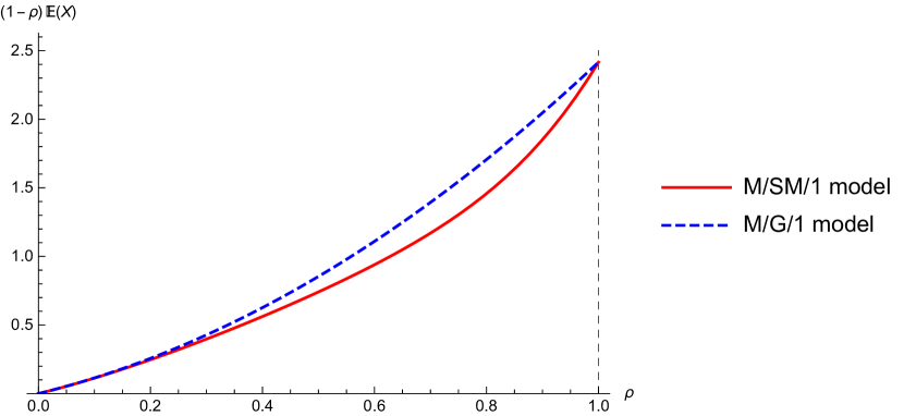
Figure 1: The mean scaled queue length versus the number of arrivals per time unit.

Indeed, it can be observed in Figure 1 that the HT limits of the mean queue lengths in both models, with and without correlated service times, are the same. Note that the light-traffic limits, when $\rho\downarrow 0$, are also the same. This, however, is caused by the fact that we chose an example with single arrivals. In the batch arrival case, the queue-length distributions would also be different in light traffic, due to the correlation between service times of customers inside one batch. It is interesting to see, however, that when $\rho$ tends to $1$, the dependence between subsequent service times no longer influences the mean scaled queue length, and thus the system can be analyzed as an $M/G/1$ queueing system, in this particular example. Furthermore, in Figure 2, it can be seen that the density of the scaled queue length converges to the limiting density of an exponential distribution when the traffic intensity $\rho$ approaches $1$.

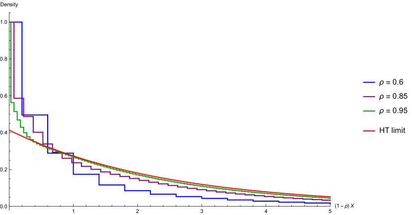
Figure 2: The density of the scaled queue length.

References

• [1] Abhishek, M. A. A. Boon, O. J. Boxma, and R. Núñez Queija. A single server queue with batch arrivals and semi-Markov services. Queueing Systems, 86(3–4):217–240, 2017.
• [2] Abhishek, M. A. A. Boon, and M. R. H. Mandjes. Generalized gap acceptance models for unsignalized intersections. submitted for publication. ArXiv report, University of Amsterdam, 2018.
• [3] Abhishek, M. A. A. Boon, and R. Núñez Queija. Applications of the $m^{x}/\text{semi-Markov}/1$ queue to road traffic. ArXiv report, University of Amsterdam, 2018.
• [4] S. Asmussen. The heavy traffic limit of a class of Markovian queueing models. Operations Research Letters, 6(6):301–306, 1987.
• [5] D. Y. Burman and S. D. R. An asymptotic analysis of a queueing system with Markov-modulated arrivals. Operations Research, 34(1):105–119, 1986.
• [6] E. Çinlar. Time dependence of queues with semi-Markovian services. J. Appl. Probab., 4:356–364, 1967.
• [7] C. F. Daganzo. Traffic delay at unsignalized intersections: clarification of some issues. Transportation Science, 11(2):180–189, 1977.
• [8] M. Dimitrov. Single-server queueing system with Markov-modulated arrivals and service times. Pliska Stud. Math. Bulgar., 20:53–62, 2011.
• [9] G. Falin and A. Falin. Heavy traffic analysis of M/G/1 type queueing systems with Markov-modulated arrivals. Sociedad de Estadistica e Investigacion Operativa Top, 7(2):279–291, 1999.
• [10] D. P. Gaver. A comparison of queue disciplines when service orientation times occur. Naval Res. Logist. Quart., 10:219–235, 1963.
• [11] M. F. Neuts. The single server queue with Poisson input and semi-Markov service times. J. Appl. Probab., 3:202–230, 1966.
• [12] M. F. Neuts. The ${M/G/1}$ queue with several types of customers and change-over times. Adv. in Appl. Probab., 9:604–644, 1977.
• [13] M. F. Neuts. Some explicit formulas for the steady-state behavior of the queue with semi-Markovian service times. Adv. in Appl. Probab., 9:141–157, 1977.
• [14] H. Thorsdottir and I. M. Verloop. Markov-modulated M/G/1-type queue in heavy traffic and its application to time-sharing disciplines. Queueing Systems, 83:29–55, 2016.
• [15] P. D. Welch. On a generalized m/g/1 queuing process in which the first customer of each busy period receives exceptional service. Operations Research, 12(5):736–752, 1964.
• [16] G. F. Yeo. Single server queues with modified service mechanisms. Journal of the Australian Mathematical Society, 2(4):499–507, 1962.