Viscous-elastic dynamics of power-law fluids within an elastic cylinder

Abstract

In a wide range of applications, microfluidic channels are implemented in soft substrates. In such configurations, where fluidic inertia and compressibility are negligible, the propagation of fluids in channels is governed by a balance between fluid viscosity and elasticity of the surrounding solid. The viscous-elastic interactions between elastic substrates and non-Newtonian fluids are particularly of interest due to the dependence of viscosity on the state of the system. In this work, we study the fluid-structure interaction dynamics between an incompressible non-Newtonian fluid and a slender linearly elastic cylinder under the creeping flow regime. Considering power-law fluids and applying the thin shell approximation for the elastic cylinder, we obtain a non-homogeneous p-Laplacian equation governing the viscous-elastic dynamics. We present exact solutions for the pressure and deformation fields for various initial and boundary conditions for both shear-thinning and shear-thickening fluids. We show that in contrast to Stokes’ problem where a compactly supported front is obtained for shear-thickening fluids, here the role of viscosity is inversed and such fronts are obtained for shear-thinning fluids. Furthermore, we demonstrate that for the case of a step in inlet pressure, the propagation rate of the front has a $t^{\frac{n}{n+1}}$ dependence on time ($t$), suggesting the ability to indirectly measure the power-law index ($n$) of shear-thinning liquids through measurements of elastic deformation.

I Introduction

Viscous-elastic interaction (VEI) is a sub-field of fluid-structure interaction focused on fluid motion at low-Reynolds numbers DupratStone . VEI received considerable attention over recent years due to its relevance to a wide spectrum of natural processes and applications. These include biological flows Ku ; Nichols , geophysical and geological flows Hewitt2015 , suppression of viscous fingering instabilities Pihler-Puzovic2012 ; Pihler-Puzovic2013 ; AlHousseiny ; Pihler-Puzovic2014 ; Pihler-Puzovic2015 ; Peng2015 , manufacturing of micro-electro-mechanical systems Hosoi2004 ; Lister2013 , development of flexible microfluidic valves Holmes , and soft robotics Shepherd ; Martinez ; Marchese ; Matia .

In particular, the case of Newtonian viscous flow through elastic channels has been extensively studied as a model problem for internal VEI flows such as those found in veins and arteries Canic , collapsible tubes (see Grotberg ; Heil and DupratStone , ch. 8, and references therein), and soft actuators Elbaz2014 . In the field of micro and nano-fluidics, channels are often fabricated from flexible materials (e.g. PDMS), which deform under internal or external pressures Hardy ; deRutte . While many microfluidic applications involve non-Newtonian fluids, very few studies examined the deformation field and flow of non-Newtonian fluids within elastic configurations. In addition to an academic interest in such systems, we believe they hold potential for novel applications, particularly in soft robotics and soft lab-on-a-chip systems, where the choice of fluid properties could allow new modes of actuation and flow control.

In this work, we extend the recent study of Elbaz and Gat Elbaz2014 which focused on Newtonian fluids, and analyze the viscous-elastic dynamics of non-Newtonian power-law fluids flowing through a slender linearly elastic cylinder. In Sec. II, we present the problem formulation as well as the key assumptions we use in the derivation of the model. In Sec. III we apply the lubrication approximation to the flow equations and the thin shell approximation to the elasticity equations and derive a non-linear p-Laplacian governing equation for the viscous-elastic dynamics. We provide appropriate scaling for physical variables and clarify the range of validity of the model. In Sec. IV we examine the viscous-elastic dynamics of the system, subjected to various initial and boundary conditions, and obtain both exact and numerical solutions for the pressure and deformation fields for both shear-thinning and shear-thickening fluids. In Sec. V we demonstrate and discuss the inverse role of viscosity in the p-Laplacian equation governing the viscous-elastic problem, as compared to Stokes’ problems Pascal1992 ; Ai ; Pritchard . We conclude with a discussion of the results in Sec. VI.

II Problem formulation

We study the low-Reynolds number fluid-structure interaction dynamics of non-Newtonian, incompressible, axisymmetric flow through a slender linearly elastic cylinder. Figure 1 presents a schematic illustration of the configuration and coordinate system. We hereafter denote dimensional variables by tildes, normalized variables without tildes and characteristic values by an asterisk superscript.

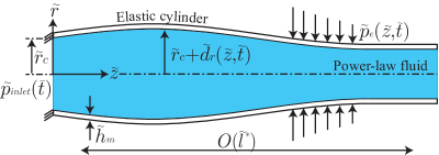
Figure 1: Schematic illustration of the examined configuration, showing the coordinate system and relevant physical parameters. An elastic cylinder of inner radius $\tilde{r}_{c}$ and wall thickness $\tilde{h}_{m}$ is clamped at $\tilde{z}=0$ and contains a non-Newtonian power-law fluid. Viscous-elastic interaction between the fluid and the elastic structure, induced by externally applied pressures $\tilde{p}_{inlet}$ and $\tilde{p}_{e}$ at the inlet and the outer boundary respectively, leads to radial, $\tilde{d}_{r}$, and axial, $\tilde{d}_{z}$, displacement fields of the elastic cylinder.

We employ a cylindrical coordinate system $(\tilde{r},\tilde{\theta},\tilde{z})$ whose $\tilde{z}$ axes coincides with the symmetry line of the cylinder. The elastic cylinder is clamped at $\tilde{z}=0$, and has an initial uniform radius $\tilde{r}_{c}$, constant wall thickness $\tilde{h}_{m}$, Young’s modulus $\tilde{E}$ and Poisson’s ratio $\nu$. The fluid’s density is $\tilde{\rho}$ and is assumed to be constant, its velocity is $\mathbf{\tilde{\mathrm{\mathit{\bm{u}}}}}=\left(\tilde{u}_{r},\tilde{u}_{z}\right)$ and its pressure is $\tilde{p}$. The externally applied pressures $\tilde{p}_{inlet}$ and $\tilde{p}_{e}$ at the inlet and the outer shell boundary, result in viscous-elastic interaction between the non-Newtonian fluid and the elastic cylinder, which in turn leads to both radial, $\tilde{d}_{r}$, and axial, $\tilde{d}_{z}$, deformation fields. The characteristic length scale in the $\bm{\hat{z}}$ direction is denoted by $\tilde{l}^{*}$, while $\tilde{d}_{r}^{*}$ and $\tilde{d}_{z}^{*}$ are the characteristic radial and axial deformations, respectively.

We further assume a slender geometry, thin walls, negligible fluidic inertia effects (small Womersley number), and small deformations in both the radial and axial directions. These can be summarized as

$$\epsilon_{1}=\frac{\tilde{r}_{c}}{\tilde{l}^{*}}\ll 1,\quad\epsilon_{2}=\frac{\tilde{h}_{m}}{\tilde{r}_{c}}\ll 1,\quad Wo\ll 1,\quad\epsilon_{3}=\frac{\tilde{d}_{r}^{*}}{\tilde{r}_{c}}\sim\frac{\tilde{d}_{z}^{*}}{\tilde{l}^{*}}\ll 1,$$ (1)

allowing the use of lubrication and thin elastic shell approximations. The exact expression for the Womersley number appearing in (1) depends on the viscosity model, which we will define in (12). Furthermore, defining both ratios, $\tilde{d}_{r}^{*}/\tilde{r}_{c}$ and $\tilde{d}_{z}^{*}/\tilde{l}^{*}$, to be of scale $\epsilon_{3}$ emanates from mass conservation of the fluid and the constitutive law of the elastic structure, as shown in the following section.

III Viscous-elastic governing equations for power-law fluids

III.1 Fluidic problem

Description of the non-Newtonian fluid rheology requires the use of a specific constitutive model. Of all models, the commonly used power-law model approximately describes the behavior of shear-dependent non-Newtonian fluids over an intermediate range of shear rates, and at the same time is sufficiently simple to allow analytical treatment. Therefore, throughout this work we consider the following constitutive model for the viscosity $\tilde{\eta}$ Bird

$$\tilde{\eta}(\dot{\gamma})=\tilde{\mu}_{eff}\dot{\gamma}^{n-1},$$ (2)

where $n$ is the dimensionless power-law index, $\tilde{\mu}_{eff}$ is the effective constant viscosity with units $\mathrm{Pa\,s^{n}}$ and $\dot{\gamma}$ is the shear rate defined as $\dot{\gamma}=\sqrt{2\bm{\tilde{D}}:\bm{\tilde{D}}},$ where $\bm{\tilde{D}}$ is the rate of deformation tensor given by $\bm{\tilde{D}}=(\bm{\tilde{\nabla}\tilde{u}}+\bm{\tilde{\nabla}\tilde{u}^{\dagger}})/2.$ The power-law index lies in the range $0<n<1$ for shear-thinning fluids, and $n>1$ for shear-thickening fluids, while $n=1$ represents the case of a Newtonian fluid.

Based on the assumptions mentioned above, the relevant governing equations and boundary conditions are the continuity equation

$$\frac{1}{\tilde{r}}\frac{\partial}{\partial\tilde{r}}\left(\tilde{r}\tilde{u}_{r}\right)+\frac{\partial\tilde{u}_{z}}{\partial\tilde{z}}=0,$$ (3)

the momentum equation in the $\bm{\hat{z}}$ direction

$$\tilde{\rho}\left(\frac{\partial\tilde{u}_{z}}{\partial\tilde{t}}+\tilde{u}_{r}\frac{\partial\tilde{u}_{z}}{\partial\tilde{r}}+\tilde{u}_{z}\frac{\partial\tilde{u}_{z}}{\partial\tilde{z}}\right)=-\frac{\partial\tilde{p}}{\partial\tilde{z}}+\frac{\partial}{\partial\tilde{z}}\left(\tilde{\tau}_{zz}\right)+\frac{1}{\tilde{r}}\frac{\partial}{\partial\tilde{r}}\left(\tilde{r}\tilde{\tau}_{rz}\right),$$ (4)

the momentum equation in the $\bm{\hat{r}}$ direction

$$\tilde{\rho}\left(\frac{\partial\tilde{u}_{r}}{\partial t}+\tilde{u}_{r}\frac{\partial\tilde{u}_{r}}{\partial\tilde{r}}+\tilde{u}_{z}\frac{\partial\tilde{u}_{r}}{\partial\tilde{z}}\right)=-\frac{\partial\tilde{p}}{\partial\tilde{r}}+\frac{1}{\tilde{r}}\frac{\partial}{\partial\tilde{r}}\left(\tilde{r}\tilde{\tau}_{rr}\right)+\frac{\partial}{\partial\tilde{z}}\left(\tilde{\tau}_{zr}\right)-\frac{\tilde{\tau}_{\theta\theta}}{\tilde{r}},$$ (5)

the constitutive equation for the stress tensor $\bm{\tilde{\tau}}$ of power-law fluid

$$\tilde{\bm{\tau}}=2\tilde{\mu}_{eff}\dot{\gamma}^{n-1}\tilde{\bm{D}},$$ (6)

as well as the no-slip and the no-penetration conditions at the solid-liquid interface

$$\tilde{u}_{z}|_{\tilde{r}=\tilde{r}_{c}+\tilde{d}_{r}}=\frac{\partial\tilde{d_{z}}}{\partial\tilde{t}},\quad\tilde{u}_{r}|_{\tilde{r}=\tilde{r}_{c}+\tilde{d}_{r}}=\frac{\partial\tilde{d_{r}}}{\partial\tilde{t}}+\tilde{u}_{z}|_{\tilde{r}=\tilde{r}_{c}+\tilde{d}_{r}}\frac{\partial d_{r}}{\partial z},$$ (7)

where $\tilde{t}$ is the time.

Scaling by the characteristic dimensions, we define the normalized coordinates, $(r,z)=(\tilde{r}/\tilde{r}_{c},\tilde{z}/\tilde{l}^{*})$, normalized velocity, $(u_{r},u_{z})=(\tilde{u}_{r}/\tilde{u}_{r}^{*},\tilde{u}_{z}/\tilde{u}_{z}^{*})$, normalized pressure, $p=\tilde{p}/\tilde{p}^{*}$, and normalized time, $t=\tilde{t}/\tilde{t}^{*}$, where $\tilde{t}^{*}$ is a characteristic time scale, $\tilde{p}^{*}$ is a characteristic pressure, $\tilde{u}_{r}^{*}$ and $\tilde{u}_{r}^{*}$ are radial and axial characteristic velocities, respectively.

Substituting the normalized parameters into the continuity equation (3), order of magnitude analysis yields the balance between radial and axial velocities

$$\frac{\tilde{u}_{r}^{*}}{\tilde{u}_{z}^{*}}\sim\frac{\tilde{r}_{c}}{\tilde{l}^{*}}=\epsilon_{1},$$ (8)

and suggests the scaling for shear rate, $\dot{\gamma}$ ,

$$\dot{\gamma}\sim\frac{\tilde{u}_{z}^{*}}{\tilde{r}_{c}}\left(\left|\frac{\partial u_{z}}{\partial r}\right|+O(\epsilon_{1}^{2})\right).$$ (9)

Order of magnitude analysis of the boundary conditions (7) yields the characteristic viscous-elastic times scale

$$\tilde{t}^{*}\sim\frac{\tilde{d}_{z}^{*}}{\tilde{u}_{z}^{*}}\sim\frac{\tilde{d}_{r}^{*}}{\tilde{u}_{r}^{*}}.$$ (10)

Substituting (8) into (4) and performing order of magnitude analysis, we obtain the axial characteristic velocity in terms of the characteristic pressure

$$\tilde{u}_{z}^{*}=\frac{\epsilon_{1}^{1+1/n}\tilde{p}^{*1/n}\tilde{l}^{*}}{\tilde{\mu}_{eff}^{1/n}},$$ (11)

as well as the condition for a negligible Womersley number in terms of relevant physical quantities

$$Wo=\frac{\tilde{\rho}\tilde{r}_{c}^{2}}{\tilde{\eta}(\dot{\gamma})\tilde{t}^{*}}=\frac{\epsilon_{1}}{\epsilon_{3}}\frac{\tilde{\rho}\tilde{u}_{z}^{*2-n}\tilde{r}_{c}^{n}}{\tilde{\mu}_{eff}}=\frac{\tilde{\rho}\tilde{u}_{z}^{*2-n}\tilde{r}_{c}^{n+1}}{\tilde{\mu}_{eff}d_{z}^{*}}\ll 1,$$ (12)

representing the ratio between the inertial-viscous time scale $\tilde{\rho}\tilde{r}_{c}^{2}/\tilde{\eta}(\dot{\gamma})=\tilde{\rho}\tilde{r}_{c}^{2}/\tilde{\mu}_{eff}(\tilde{u}_{z}^{*}/\tilde{r}_{c})^{n-1}$ and the viscous-elastic time scale $\tilde{t}^{*}=\tilde{d}_{z}^{*}/\tilde{u}_{z}^{*}.$

Substituting (8)-(12) into (3)-(7) and applying the lubrication approximation results in the following set of normalized equations and boundary conditions,

$$\frac{1}{r}\frac{\partial}{\partial r}\left(ru_{r}\right)+\frac{\partial u_{z}}{\partial z}=0,$$ (13)

$$\frac{\partial p}{\partial z}=\frac{1}{r}\frac{\partial}{\partial r}\left(r\left|\frac{\partial u_{z}}{\partial r}\right|^{n-1}\frac{\partial u_{z}}{\partial r}\right)+O(Wo,\epsilon_{1}^{2}),$$ (14)

$$\frac{\partial p}{\partial r}=O(\epsilon_{1}^{2}Wo,\epsilon_{1}^{2}),$$ (15)

and

$$u_{z}|_{r=1+\epsilon_{3}d_{r}}=\frac{\partial d{}_{z}}{\partial t},\quad u_{r}|_{r=1+\epsilon_{3}d_{r}}=\frac{\partial d_{r}}{\partial t}+\epsilon_{3}\frac{\partial d{}_{z}}{\partial t}\frac{\partial d_{r}}{\partial z}.$$ (16)

Integrating (14) with respect to $r$ and applying the symmetry condition at $r=0$ yields

$$\frac{\partial u_{z}}{\partial r}=\left|\frac{\partial p}{\partial z}\right|^{\frac{1}{n}-1}\frac{\partial p}{\partial z}\left(\frac{r}{2}\right)^{\frac{1}{n}}.$$ (17)

Integrating (17) again with respect to $r$ and applying the no-slip boundary conditions (16), results in

$$u_{z}=\frac{1}{2^{\frac{1}{n}}}\frac{n}{n+1}\left|\frac{\partial p}{\partial z}\right|^{\frac{1}{n}-1}\frac{\partial p}{\partial z}\left(r^{1+\frac{1}{n}}-(1+\epsilon_{3}d_{r}(z,t))^{1+\frac{1}{n}}\right)+\frac{\partial d_{z}}{\partial t}.$$ (18)

Defining volume flux as $q=2\pi\int_{r=0}^{r=1+\epsilon_{3}d_{r}}ru_{z}dr$, from (18) it follows

$$\frac{q}{2\pi}=\int_{r=0}^{r=1+\epsilon_{3}d_{r}}ru_{z}dr=-\frac{1}{2^{\frac{1+n}{n}}}\frac{n}{3n+1}\left|\frac{\partial p}{\partial z}\right|^{\frac{1}{n}-1}\frac{\partial p}{\partial z}+\frac{1}{2}\frac{\partial d_{z}}{\partial t}+O(\epsilon_{3}).$$ (19)

Utilizing (16) and (19), and then integrating (13) with respect to $r$, we relate the pressure and deformation fields

$$\frac{\partial d_{r}}{\partial t}+\frac{\partial}{\partial z}\left(-\frac{1}{2^{\frac{1+n}{n}}}\frac{n}{3n+1}\left|\frac{\partial p}{\partial z}\right|^{\frac{1}{n}-1}\frac{\partial p}{\partial z}+\frac{1}{2}\frac{\partial d_{z}}{\partial t}\right)=0.$$ (20)

III.2 Elastic problem

A similar elastic configuration was considered by Elbaz and Gat Elbaz2014 , who provided relations between the pressure and deformation fields. For completeness, we here present the governing equations and these key relations, adapted to our notation.

Focusing on viscous-elastic time scales which are typically significantly longer than elastic inertial time scales, and further neglecting body forces, the deformation field of an axisymmetric linearly elastic material is described by the momentum equations in the $\bm{\hat{r}}$ and $\bm{\hat{z}}$ directions (see Timoshenko, ; Howell, ),

$$\frac{\partial}{\partial\tilde{r}}\left(\tilde{r}\tilde{\sigma}_{rr}\right)+\frac{\partial}{\partial\tilde{z}}\left(\tilde{r}\tilde{\sigma}_{rz}\right)-\tilde{\sigma}_{\theta\theta}=0,\quad\frac{\partial}{\partial\tilde{r}}\left(\tilde{r}\tilde{\sigma}_{rz}\right)+\frac{\partial}{\partial\tilde{z}}\left(\tilde{r}\tilde{\sigma}_{zz}\right)=0,$$ (21)

the strain-displacement relations for small deformations,

$$\tilde{e}_{rr}=\frac{\partial\tilde{d}_{r}}{\partial\tilde{r}},\quad\tilde{e}_{\theta\theta}=\frac{\tilde{d}_{r}}{\tilde{r}},\quad\tilde{e}_{zz}=\frac{\partial\tilde{d}_{z}}{\partial\tilde{z}},\quad\tilde{e}_{rz}=\frac{1}{2}\left(\frac{\partial\tilde{d}_{r}}{\partial\tilde{z}}+\frac{\partial\tilde{d}_{z}}{\partial\tilde{r}}\right),$$ (22)

and Hooke’s law,

$$\tilde{e}_{rr}=\frac{1}{\tilde{E}}\left(\tilde{\sigma}_{rr}-\nu\left(\tilde{\sigma}_{zz}+\tilde{\sigma}_{\theta\theta}\right)\right),\quad\tilde{e}_{\theta\theta}=\frac{1}{\tilde{E}}\left(\tilde{\sigma}_{\theta\theta}-\nu\left(\tilde{\sigma}_{zz}+\tilde{\sigma}_{rr}\right)\right),$$ (23a)

$$\tilde{e}_{zz}=\frac{1}{\tilde{E}}\left(\tilde{\sigma}_{zz}-\nu\left(\tilde{\sigma}_{\theta\theta}+\tilde{\sigma}_{rr}\right)\right),\quad\tilde{e}_{rz}=\frac{1+\nu}{\tilde{E}}\tilde{\sigma}_{rz}.$$ (23b)

The governing equations (21) are subjected to the following boundary conditions applied by the liquid

$$\tilde{\sigma}_{rr}|_{\tilde{r}=\tilde{r}_{c}+\tilde{d}_{r}}=-\tilde{p}+2\tilde{\mu}_{eff}\dot{\gamma}^{n-1}\frac{\partial\tilde{u}_{r}}{\partial\tilde{r}},\quad\tilde{\sigma}_{rz}|_{\tilde{r}=\tilde{r}_{c}+\tilde{d}_{r}}=\tilde{\mu}_{eff}\dot{\gamma}^{n-1}\left(\frac{\partial\tilde{u}_{z}}{\partial\tilde{r}}+\frac{\partial\tilde{u}_{r}}{\partial\tilde{z}}\right),$$ (24)

and the external stress

$$\tilde{\sigma}_{rr}|_{\tilde{r}=\tilde{r}_{c}+\tilde{d}_{r}+\tilde{h}_{m}}=-\tilde{p}_{e},\quad\tilde{\sigma}_{rz}|_{\tilde{r}=\tilde{r}_{c}+\tilde{d}_{r}+\tilde{h}_{m}}=0.$$ (25)

We follow the derivation of Elbaz and Gat Elbaz2014 and obtain the normalized governing equations for the radial and axial deformations in terms of the pressure

$$d_{r}(z,t)=\left(1-\frac{\nu}{2}\right)p(z,t)-p_{e},\quad d_{z}(z,t)=\int_{0}^{z}\left[(\frac{1}{2}-\nu)p(z,t)+\nu p_{e}\right]dz,$$ (26)

as well as the characteristic radial deformation, $\tilde{d}_{r}^{*}$, in terms of characteristic pressure

$$\frac{\tilde{d}_{r}^{*}}{\tilde{r}_{c}}=\frac{\tilde{p}^{*}}{\epsilon_{2}\tilde{E}}\ll 1.$$ (27)

In the Supplemental Material SI , we show that early scaling of the radial differential, $d\tilde{r}$, in (21) by $\tilde{h}_{m}$ (instead of $\tilde{r}_{c}$ (see Elbaz2014, )) is a more natural choice which leads to significant simplification in the derivation of (26) and (27) in the current configuration.

III.3 P-Laplacian equation governing the pressure field and its asymptotic approximation

To combine the fluidic and elastic problems, we substitute elastic relation (26) into the fluidic relation (20), resulting in a single equation in terms of the pressure

$$\frac{\partial p}{\partial t}-\frac{\partial}{\partial z}\left(\left|\frac{\partial p}{\partial z}\right|^{\frac{1}{n}-1}\frac{\partial p}{\partial z}\right)=\frac{4-2\nu}{5-4\nu}\frac{\partial p_{e}}{\partial t},$$ (28)

subjected to the following initial and boundary conditions

$$p(z,t=0)=p_{initial}(z),\quad p(z=0,t)=p_{inlet}(t),$$ (29)

where, for the convenience, we have rescaled the time, $t$, according to

$$t\rightarrow\frac{t}{\alpha},\quad\alpha\triangleq\frac{1}{5-4\nu}\frac{1}{2^{\frac{1-n}{n}}}\frac{n}{3n+1}.$$ (30)

Equation (28) is a non-homogeneous one dimensional p-Laplacian equation describing the pressure in an elastic cylinder containing a power-law fluid subjected to external forcing.

Similar p-Laplacian equations are encountered in other problems involving the use of non-Newtonian power-law fluids. For example, the p-Laplacian equation represents balance between compressibility and viscosity for the flow of a weakly compressible non-Newtonian fluid in a porous medium Pascal1985 ; Pascal1991 ; DiFederico , as well as a balance between viscosity and inertia in Stokes’ first Pascal1992 ; Duffy and second problems Ai ; Pritchard , where the operator is applied to the fluid velocity. We here rely on the previous mathematical analysis of the p-Laplacian equation to provide insight into our viscous-elastic problem, such as self-similarity and compact support of the solutions for pressure and deformation fields.

For the case of a non-Newtonian power-law fluid that exhibits a weak shear-thinning or shear-thickening behavior, we follow Ross, Wilson and Duffy Ross and define the auxiliary small parameter $\varepsilon$,

$$n=1-\varepsilon,$$ (31)

and the asymptotic expansion

$$p=p^{(0)}+\varepsilon p^{(1)}+O(\varepsilon^{2}),$$ (32)

where $\left|\varepsilon\right|\ll 1$ is a small parameter which is positive for shear-thinning and negative for shear-thickening behaviors. Using (31) and (32) the expansion $1/n\sim 1+\varepsilon+O(\varepsilon^{2})$, yields

$$\left|\frac{\partial p}{\partial z}\right|^{\frac{1}{n}-1}=1+\varepsilon\ln\left|\frac{\partial p^{(0)}}{\partial z}\right|+O(\varepsilon^{2}).$$ (33)

We note that the expansion (33) is valid only provided the leading-order pressure gradient is non-zero and bounded throughout the domain. Utilizing (31)-(33), we obtain the leading-order and first-order corrections of the governing equation (28)

$$O(1):\quad\frac{\partial p^{(0)}}{\partial t}-\frac{\partial^{2}p^{(0)}}{\partial z^{2}}=\frac{4-2\nu}{5-4\nu}\frac{\partial p_{e}}{\partial t},$$ (34)

and

$$O(\varepsilon):\quad\frac{\partial p^{(1)}}{\partial t}-\frac{\partial^{2}p^{(1)}}{\partial z^{2}}=\frac{\partial}{\partial z}\left(\ln\left|\frac{\partial p^{(0)}}{\partial z}\right|\frac{\partial p^{(0)}}{\partial z}\right).$$ (35)

Both (34) and (35) are parabolic equations where the inhomogeneous part of (34) is related to the external forcing (see Elbaz2014, ), and the inhomogeneous part of (35) emanates from the non-Newtonian response of the fluid to the leading-order pressure gradients.

III.4 Characteristic physical parameters and model range of validity

We here summarize the characteristic values of relevant physical parameters and the range of validity of the current model. From order of magnitude analysis, the characteristic length scale $\tilde{l}^{*}$, the characteristic axial velocity $\tilde{u}_{z}^{*}$, and the characteristic deformations $\tilde{d}_{r}^{*}$ and $\tilde{d}_{z}^{*}$ are given by

$$\tilde{l}^{*}=\left(\alpha\frac{\tilde{E}\tilde{h}_{m}\tilde{t}^{*}}{\tilde{p}^{*}}\right)^{\frac{n}{n+1}}\left(\frac{\tilde{p}^{*}\tilde{r}_{c}}{\tilde{\mu}_{eff}}\right)^{\frac{1}{n+1}},$$ (36a)

$$\tilde{u}_{z}^{*}=\tilde{r}_{c}\left(\frac{\tilde{p}^{*}}{\tilde{\mu}_{eff}}\frac{\tilde{r}_{c}}{\tilde{l}^{*}}\right)^{\frac{1}{n}},$$ (36b)

$$\tilde{d}_{r}^{*}=\tilde{r}_{c}\frac{\tilde{r}_{c}}{\tilde{h}_{m}}\frac{\tilde{p}^{*}}{\tilde{E}},$$ (36c)

and

$$\tilde{d}_{z}^{*}=\tilde{l}^{*}\frac{\tilde{r}_{c}}{\tilde{h}_{m}}\frac{\tilde{p}^{*}}{\tilde{E}}.$$ (36d)

Since in this work we focus on semi-infinite configuration, there is no inherent axial length scale to the problem and thus scaling analysis provides only a relation between $\tilde{l}^{*}$ and $\tilde{t}^{*}$. We define the characteristic pressure $\tilde{p}^{*}$ and the characteristic time scale $\tilde{t}^{*}$ from the boundary condition $\tilde{p}(0,\tilde{t})=\tilde{p}_{inlet}(\tilde{t})$ with characteristic amplitude $\tilde{p}_{0}$ and time scale $\tilde{t}_{0}$, by setting $\tilde{p}^{*}=\tilde{p}_{0}$ and $\tilde{t}^{*}=\tilde{t}_{0}$.

Substituting (36a)-(36d) into (1) provides formulation of the assumptions made in the model in terms of known physical and geometrical parameters:

$$\epsilon_{1}=\tilde{r}_{c}\left(\alpha\frac{\tilde{E}\tilde{h}_{m}\tilde{t}_{0}}{\tilde{p}_{0}}\right)^{-\frac{n}{n+1}}\left(\frac{\tilde{p}_{0}\tilde{r}_{c}}{\tilde{\mu}_{eff}}\right)^{-\frac{1}{n+1}}\ll 1,$$ (37a)

$$\epsilon_{2}=\frac{\tilde{h}_{m}}{\tilde{r}_{c}}\ll 1,$$ (37b)

$$\epsilon_{3}=\frac{\tilde{d}_{r}^{*}}{\tilde{r}_{c}}=\frac{\tilde{d}_{z}^{*}}{\tilde{l}^{*}}=\frac{\tilde{r}_{c}}{\tilde{h}_{m}}\frac{\tilde{p}_{0}}{\tilde{E}}\ll 1,$$ (37c)

$$Wo=\frac{\tilde{\rho}\tilde{r}_{c}^{2}}{\tilde{\mu}_{eff}\tilde{t}_{0}}\left(\alpha\frac{\tilde{h}_{m}}{\tilde{r}_{c}}\frac{\tilde{E}}{\tilde{p}_{0}}\frac{\tilde{t}_{0}\tilde{\mu}_{eff}}{\tilde{p}_{0}}\right)^{\frac{n-1}{n+1}}\ll 1.$$ (37d)

Property	Symbol	Value	Units	Based on
Wall thickness	$\tilde{h}_{m}$	50	$\mu m$	input
Inner radius	$\tilde{r}_{c}$	500	$\mu m$	input
Young’s modulus (PDMS)	$\tilde{E}$	$1\times 10^{6}$	Pa	input
Poisson’s ratio	$\nu$	0.3	–	input
Power-law index (Xanthan suspension)	$n$	$0.55$	–	input
Effective viscosity (Xanthan suspension)	$\tilde{\mu}_{eff}$	0.57	Pa sn	input
Characteristic time scale	$\tilde{t}^{*}$	0.5	s	input
Characteristic pressure	$\tilde{p}^{*}$	$1\times 10^{4}$	Pa	input
Axial length scale	$\tilde{l}^{*}$	$14$	cm	(36a)
Typical axial velocity	$\tilde{u}_{z}^{*}$	0.91	$\mathrm{m\,s^{-1}}$	(36b)
Typical radial deformation	$\tilde{d}_{r}^{*}$	50	$\mu m$	(36c)
Typical axial deformation	$\tilde{d}_{z}^{*}$	14	mm	(36d)
Slenderness	$\epsilon_{1}$	$3.5\times 10^{-3}$	–	(37a)
Wall thinness	$\epsilon_{2}$	0.1	–	(37b)
Smallness of deformations	$\epsilon_{3}$	0.1	–	(37c)
Womersley number	$Wo$	$2.5\times 10^{-2}$	–	(37d)

Table 1: Characteristic values of physical parameters corresponding to the flow of Xanthan gum suspension in a 500 $\mu m$ radius PDMS channel, subjected to external pressure of $1\times 10^{4}$ Pa. Resulting values for the non-dimensional parameters (in bold) indicate that the model holds well in this regime.

To illustrate the applicability of these assumptions in soft-robotic and lab-on a-chip applications, we examine a typical micro-configuration made of PDMS (polydimethylsiloxane, $\tilde{E}=10^{6}\,\mathrm{Pa}$, Cheng, ) and containing a suspension of Xanthan gum behaving as power-law viscous fluid ($n=0.55,\,\tilde{\mu}_{eff}=0.57\,$$\mathrm{Pa\,s^{n}}$, Longo, ). Table 1 presents the characteristic values of physical and geometric parameters, readily satisfying the assumptions used in the current analysis.

IV Results

In this section, we examine the viscous-elastic dynamics resulting from time-varying inlet pressure. We first obtain the pressure field by solving the governing equation (28) for arbitrary values of $n$. Then, using (19) and (26), we provide the corresponding volume flux and deformation field.

IV.1 Instantaneous injection of mass at the inlet

We examine the viscous-elastic dynamics due to an initial localized pressure at $z=0$, which may be represented by

$$p(z,t=0)=\delta(z),$$ (38)

where $\delta$ is Dirac’s delta function. We note that (38) physically results from instantaneous release of a fluid mass, $\tilde{m}$, into the elastic cylinder at the inlet at $t=0$ after which ($t>0$), the inlet is sealed and thus

$$\frac{\partial p}{\partial z}\left(z=0,t>0\right)=0.$$ (39)

Mass is thus conserved globally according to

$$\int_{0}^{\infty}d_{r}dz=\frac{\tilde{m}}{2\pi\tilde{\rho}\tilde{r}_{c}\tilde{l}^{*}\tilde{d}_{r}^{*}},$$ (40)

which using (26) can be rewritten as

$$\int_{0}^{\infty}pdz=\frac{\tilde{m}}{\pi\left(2-\nu\right)\tilde{\rho}\tilde{r}_{c}\tilde{l}^{*}\tilde{d}_{r}^{*}}.$$ (41)

In the following, we assume that the fluid mass, $\tilde{m}$, is such that the right-hand side of (41) is unity, $\int_{0}^{\infty}pdz=1$. Note that the conservation law, (41), can be also derived by integrating (28) with respect to $z$ from $0$ to $\infty$, using (38). Following Di Federico and Ciriello DiFederico , who focused on shear-thinning fluids and considered an instantaneous mass injection of a weakly compressible power-law fluid into porous medium, we construct self-similar solutions by defining a similarity variable $\xi$

$$\xi=zt^{-\frac{n}{2}},$$ (42)

and self-similar profile $f$

$$p(z,t)=t^{-\frac{n}{2}}f(\xi).$$ (43)

For a Newtonian fluid ($n=1$) the solution is well-known

$$p(z,t)=\frac{1}{\sqrt{\pi t}}\exp\left(-\frac{z^{2}}{4t}\right)=t^{-1/2}\frac{1}{\sqrt{\pi}}\exp\left(-\frac{\xi^{2}}{4}\right)\triangleq t^{-\frac{1}{2}}f(\xi).$$ (44)

For non-Newtonian fluids, substituting (43) into (28) and (41) yields an ordinary differential equation for the self-similar profile and the corresponding conservation law,

$$\frac{d}{d\xi}\left(\left|\frac{df(\xi)}{d\xi}\right|^{\frac{1}{n}-1}\frac{df(\xi)}{d\xi}+\frac{n}{2}\xi f(\xi)\right)=0,$$ (45)

and

$$\int_{0}^{\infty}f(\xi)d\xi=1.$$ (46)

Integrating (45) with respect to $\xi$ and applying the far-field condition of vanishing pressure and its derivatives $f=df/d\xi\rightarrow 0$ as $\xi\rightarrow\infty$, yield

$$\left|\frac{df(\xi)}{d\xi}\right|^{\frac{1}{n}-1}\frac{df(\xi)}{d\xi}+\frac{n}{2}\xi f(\xi)=0.$$ (47)

Since, the pressure should be positive and the pressure gradient should be negative, i.e. $f\geq 0$ and $df/d\xi\leq 0$, we can drop the absolute value in (47) and obtain

$$\frac{df}{d\xi}=-\left(\frac{n}{2}\right)^{n}\xi^{n}f(\xi)^{n}<0.$$ (48)

Integrating (48) with respect to $\xi$ leads to

$$f(\xi)=\xi_{*}^{\frac{1+n}{1-n}}\left|k\right|^{\frac{1}{1-n}}\left(1\mp\frac{\xi^{n+1}}{\xi_{*}^{n+1}}\right)_{+}^{\frac{1}{1-n}},$$ (49)

where the minus and plus signs stand for $n<1$ and $n>1$, respectively, $k$ is defined as

$$k=\left(\frac{n}{2}\right)^{n}\frac{1-n}{1+n},$$ (50)

$x_{+}=\max\left\{x,0\right\}$ and $\xi_{*}$ is a positive constant uniquely determined from (46) and given by

$$\xi_{*}=\left\{\begin{array}[]{ll}\xi_{front}=\left(\frac{1}{\left|k\right|^{\frac{1}{1-n}}}\frac{\Gamma(\frac{3-n^{2}}{1-n^{2}})}{\Gamma(\frac{2-n}{1-n})\Gamma(\frac{2+n}{1+n})}\right)^{\frac{1-n}{2}}&n<1\\ \xi_{no\,front}=\left(\frac{1}{\left|k\right|^{\frac{1}{1-n}}}\frac{\Gamma(\frac{1}{n-1})}{\Gamma(\frac{2}{n^{2}-1})\Gamma(\frac{2+n}{1+n})}\right)^{\frac{1-n}{2}}&n>1\end{array},\right.$$ (51)

where $\Gamma$ is the Gamma function Abramowitz .

For a shear-thinning fluid, $n<1$, the self-similar profile $f(\xi)$ becomes uniformly zero for $\xi>\xi_{front}$ thus indicating the existence of a front which moves according to $z_{front}(t)=\xi_{front}t^{\frac{n}{2}}$. The condition $f=df/d\xi\rightarrow 0$ holds now at $\xi=\xi_{front}$. In contrast to the shear-thinning fluid, the self-similar profile $f(\xi)$ of the shear-thickening fluid, $n>1$, approaches zero only as $\xi\rightarrow\infty$, similarly to the case of a Newtonian fluid.

The closed-form solutions, (49), provide the associated radial deformation

$$d_{r}(z,t)=\left(1-\frac{\nu}{2}\right)p(z,t)=\left(1-\frac{\nu}{2}\right)t^{-\frac{n}{2}}f(\xi),$$ (52)

which admits the same self-similar profile $f$. Substituting (44) and (49) into (26), we obtain the corresponding self-similar axial deformation in the form $d_{z}(z,t)=\left(0.5-\nu\right)\int_{0}^{z}p(z,t)dz=\left(0.5-\nu\right)D_{z}(\xi)$, where $D_{z}(\xi)$ is expressed in terms of generalized hyper-geometric functions

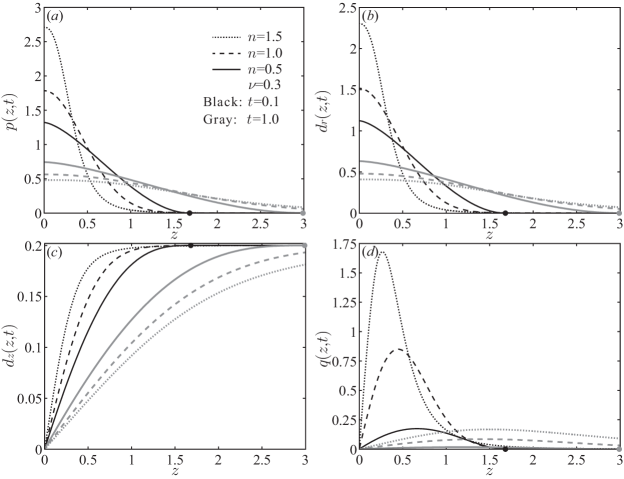
Figure 2: Propagation of a power-law fluid in an elastic cylinder due to instantaneous injection of mass at $z=0$. (a) and (b) present, respectively, the pressure distribution and radial deformation as a function of the axial coordinate, both of which are characterized by the decay rate of $t^{-n/2}$. (c) and (d) present, respectively, the axial deformation and volume flux as a function of the axial coordinate, both of which have a decay rate that is independent of $n$. Black and gray lines correspond to $t=0.1$ and $t=1.0$, respectively. Dotted lines represent a shear-thickening fluid ($n=1.5)$, dashed lines represent a Newtonian fluid ($n=1)$ and solid lines represent a shear-thinning fluid ($n=0.5)$. At early times the shear-thickening fluid is more localized (but not compactly supported) than the Newtonian and shear-thinning fluids, while for longer times the shear-thinning fluid has the lowest propagation rate remaining compactly supported. Black and gray dots indicate the location of the front of shear-thinning fluid, $z_{front}(t)=2.99t^{1/4}$.

$$D_{z}(\xi)=\left\{\begin{array}[]{ll}\xi_{*}^{\frac{1+n}{1-n}}\left|k\right|^{\frac{1}{1-n}}\xi{}_{2}F_{1}\left(\frac{1}{n-1},\frac{1}{n+1};\frac{n+2}{n+1};\pm\frac{\xi^{n+1}}{\xi_{*}^{n+1}}\right)&n\neq 1\\ \mathrm{erf}\left(\frac{\xi}{2}\right)&n=1\end{array},\right.$$ (53)

where ${}_{2}F_{1}\left(a,b;c;z\right)$ is the Gaussian hyper-geometric function Abramowitz ; Slater . The plus and minus signs correspond to $n<1$ and $n>1$, respectively. Rescaling the time in the expression for the volume flux, (19), according to (30), we find

$$q=\frac{n}{3n+1}\frac{\pi}{2^{\frac{1}{n}}}\left(-\left|\frac{\partial p}{\partial z}\right|^{\frac{1}{n}-1}\frac{\partial p}{\partial z}+\frac{2}{5-4\nu}\frac{\partial d_{z}}{\partial t}\right).$$ (54)

Expressing (54) in terms of the similarity variable $\xi$ yields

$$q=\frac{n^{2}}{3n+1}\frac{\pi}{2^{\frac{1}{n}}}\frac{2-\nu}{5-4\nu}t^{-1}\xi f(\xi)=\frac{n^{2}}{3n+1}\frac{\pi}{2^{\frac{1}{n}}}\frac{2-\nu}{5-4\nu}t^{-1}Q(\xi),$$ (55)

where $f(\xi)$ is given in (44) and in (49) for the Newtonian fluid and the non-Newtonian fluid, respectively, and $Q(\xi)=\xi f(\xi)$.

Figure (2) summarizes the results of viscous-elastic interaction due to a pressure impulse applied at the inlet for $n=0.5,1,1.5$. All solutions corresponding to shear-thinning fluids are compactly supported, in contrast to solutions of Newtonian and shear-thickening fluids. Figures 2(a) and 2(b) present the pressure distribution and the radial deformation versus the axial coordinate $z$, for different times. From (43) and (52), the decay rate in this case scales as $t^{-n/2}$, thus indicating that for long times the pressure and the radial deformation of shear-thickening fluids decay (and propagate) faster than in the case of Newtonian and shear-thinning fluids, consistent with the results of Figs. 2(a) and 2(b). Figures 2(c) and 2(d) show the axial deformation and volume flux versus axial coordinate. In this case, the decay rate is similar for Newtonian and non-Newtonian fluids (i.e. is independent of $n$).

It worth to note that at early-times, $t\ll 1$, the shear-thickening fluids have the lowest propagation rate and are thus more localized (but not compactly supported) than the Newtonian and shear-thinning fluids. This is inverted at longer times as propagation rate of the shear-thickening fluids increases, and they are least localized.

Furthermore, we note that the current analysis is limited to an intermediate range of shear rates in accordance the validity range of the power-law model. For sufficiently long times, as $\partial p/\partial z$ diminishes, the shear rate will also diminish, driving the effective viscosity outside the validity range of the power-law model. Thus, the current analysis will become invalid at long times. In practice, in such cases the effective viscosity would approach a constant value, and the dynamics could be described by a linear diffusion equation.

IV.2 Sudden change of inlet pressure

We here examine the viscous-elastic dynamics associated with a sudden change of inlet pressure

$$p(z=0,t)=p_{0}H(t),$$ (56)

from an initially uniform pressure within the cylinder, $p(z,t=0)=p_{i}$. Here $H$ stands for the Heaviside function, whereas $p_{i}$ and $p_{0}$ are the magnitudes of the initial and the applied pressure, respectively. The pressure gradient is positive for $p_{i}>p_{0}$ and negative for $p_{i}<p_{0}$, corresponding to filling or discharging of the elastic tube, respectively.

For convenience, we define $\beta=\mathrm{sgn}\left(p_{i}-p_{0}\right)$ and rewrite (28) as

$$\frac{\partial p}{\partial t}-\frac{\partial}{\partial z}\left(\left(\beta\frac{\partial p}{\partial z}\right)^{\frac{1}{n}-1}\frac{\partial p}{\partial z}\right)=0.$$ (57)

Following Pascal and Pascal Pascal1985 , we define a similarity variable $\xi$

$$\xi=zt^{-\frac{n}{n+1}},$$ (58)

and require

$$p(z,t)=p(\xi).$$ (59)

The corresponding solution for a Newtonian fluid solution is

$$p(z,t)=p_{0}+\left(p_{i}-p_{0}\right)\mathrm{erf}\left(\frac{z}{2\sqrt{t}}\right),\quad p(\xi)=p_{0}+\left(p_{i}-p_{0}\right)\mathrm{erf}\left(\frac{\xi}{2}\right).$$ (60)

For the non-Newtonian case, we substitute (58) and (59) into (57), obtaining an ordinary differential equation for the pressure

$$\frac{d^{2}p(\xi)}{d\xi^{2}}+\beta\frac{n^{2}}{n+1}\xi\left(\beta\frac{dp(\xi)}{d\xi}\right)^{\frac{2n-1}{n}}=0,$$ (61)

with boundary conditions for $t>0$

$$p(\xi=0)=p_{0},\quad p(\xi\rightarrow\infty)=p_{i},\quad\frac{dp}{d\xi}(\xi\rightarrow\infty)=0.$$ (62)

Integrating once (61) with respect to $\xi$ yields

$$\frac{dp}{d\xi}=\beta\xi_{*}^{\frac{2n}{1-n}}\left|k\right|^{\frac{n}{1-n}}\left(1\mp\frac{\xi^{2}}{\xi_{*}^{2}}\right)_{+}^{\frac{n}{1-n}},$$ (63)

where the upper and lower signs correspond to $n<1$ and $n>1$, respectively. The parameter $k$ is defined as

$$k=\frac{n}{2}\frac{1-n}{1+n},$$ (64)

and $\xi_{*}$ is a constant to be determined from boundary conditions on the pressure, in contrast to Sec. IV A where a similar constant is found from conservation of mass.

Integrating (63) with respect to $\xi$ and applying the boundary condition (62) at $\xi=0$, leads to

$$p(\xi)=p_{0}+\beta\xi_{*}^{\frac{2n}{1-n}}\left|k\right|^{\frac{n}{1-n}}\xi{}_{2}F_{1}\left(\frac{1}{2},\frac{n}{n-1};\frac{3}{2};\pm\frac{\xi^{2}}{\xi_{*}^{2}}\right).$$ (65)

To determine the constant $\xi_{*}$ for different values of $n$, we utilize the boundary condition $p(\xi\rightarrow\infty)=0$, yielding

$$\xi_{*}=\left\{\begin{array}[]{ll}\xi_{front}=\left(\frac{2\left|p_{i}-p_{0}\right|}{\sqrt{\pi}\left|k\right|^{\frac{n}{1-n}}}\frac{\Gamma(\frac{n-3}{2(n-1)})}{\Gamma(\frac{1}{1-n})}\right)^{\frac{1-n}{1+n}}&n<1\\ \xi_{no\,front}=\left(\frac{2\left|p_{i}-p_{0}\right|}{\sqrt{\pi}\left|k\right|^{\frac{n}{1-n}}}\frac{\Gamma(\frac{n}{(n-1)})}{\Gamma(\frac{n+1}{2(n-1)})}\right)^{\frac{1-n}{1+n}}&n>1\end{array}.\right.$$ (66)

From (63) we obtain that for shear-thinning fluids $dp/d\xi=0$ at $\xi=\xi_{*}=\xi_{front}$, thus indicating the existence of a front moving according to $z_{front}(t)=\xi_{front}t^{n/(n+1)}$. On the other hand, for shear-thickening fluids it follows that $dp/d\xi=0$ only as $\xi\rightarrow\infty$, and therefore no front exists.

Figures 3(a) and 3(b) present the resulting pressure distribution, (65), and the radial deformation, $d_{r}(z,t)=\left(1-0.5\nu\right)p(z,t)=\left(1-0.5\nu\right)p(\xi)$, corresponding to the case of $p_{0}=1,\,p_{i}=0,\,\beta=-1$, for different times. Figure 3(c) shows the axial deformation, $d_{z}(z,t)$, given as $d_{z}(z,t)=\left(0.5-\nu\right)\int_{0}^{z}p(z,t)dz=\left(0.5-\nu\right)zD_{z}(\xi)/\xi$, where for the Newtonian fluid ($n=1$) $D_{z}(\xi)$ is the following self-similar profile,

$$D_{z}(\xi)=p_{0}\xi+\left(p_{i}-p_{0}\right)\left(\frac{2}{\sqrt{\pi}}\left(-1+\mathrm{e}^{-\xi^{2}/4}\right)+\xi\mathrm{erf}\left(\frac{\xi}{2}\right)\right),$$ (67)

and for a non-Newtonian fluid is given by

$$D_{z}(\xi) = p_{0}\xi+\beta\xi_{*}^{\frac{2n}{1-n}}\left|k\right|^{\frac{n}{1-n}}\left[\xi^{2}{}_{2}F_{1}\left(\frac{1}{2},\frac{n}{n-1};\frac{3}{2};\pm\frac{\xi^{2}}{\xi_{*}^{2}}\right)\right.$$

$$\left.+\frac{1}{2}\left(n-1\right)\xi_{*}^{2}\left(\mp\xi^{2}+\xi_{*}^{2}\right)^{\frac{n}{1-n}}\left(\xi^{2}\xi_{*}^{\frac{2}{n-1}}\mp\xi_{*}^{\frac{2n}{n-1}}\pm\left(\mp\xi^{2}+\xi_{*}^{2}\right)^{\frac{n}{n-1}}\right)\right],$$ (68)

where the upper signs in (68) correspond to $n<1$ and the lower signs correspond to $n>1$, respectively. The solution for volume flux is presented in Fig. 3(d) and is obtained using (54),

$$q=\frac{n}{3n+1}\frac{\pi}{2^{\frac{1}{n}}}t^{-\frac{1}{n+1}}\left[\left(\beta\frac{dp}{d\xi}\right)^{\frac{1}{n}}+\frac{n}{n+1}\frac{1-2\nu}{5-4\nu}\left(D_{z}(\xi)-\xi\frac{dD_{z}(\xi)}{d\xi}\right)\right],$$ (69)

where the expressions of $p(\xi)$ and $D_{z}(\xi)$ are given in (60) and (67) for the Newtonian fluid, and in (65) and (68) for the non-Newtonian fluid.

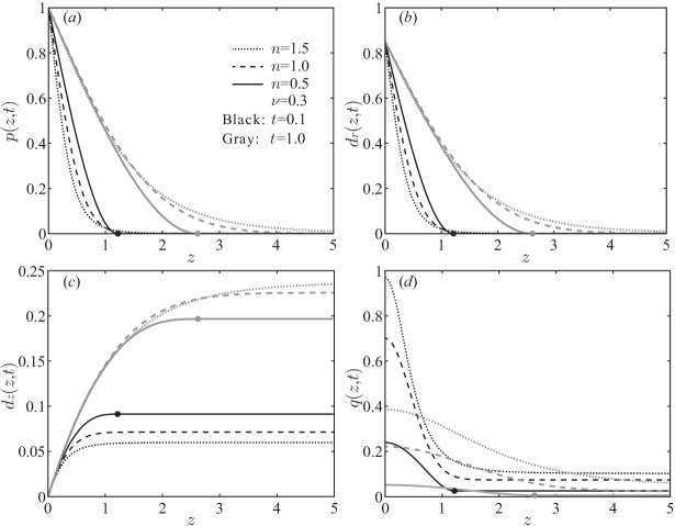
Figure 3: Viscous-elastic dynamics of power-law fluids within an elastic cylinder due to a step increase in inlet pressure. (a), (b) and (c) present, respectively, the pressure distribution and the radial and axial deformations a function of the axial coordinate. While for sufficiently long times, $t\rightarrow\infty$, the radial deformation approaches a constant value, $d_{r}\rightarrow 0.85$, the axial deformation is a linear function of $z$ with the slope of 0.2, $d_{z}/z\rightarrow 0.2$, independently of $n$. (d) shows the volume flux versus axial coordinate, characterized by the decay rate of $t^{-1/(n+1)}$. Black and gray lines correspond to $t=0.1$ and $t=1.0$, respectively. Dotted lines represent a shear-thickening fluid ($n=1.5)$, dashed lines represent a Newtonian fluid ($n=1)$ and solid lines represent a shear-thinning fluid ($n=0.5)$. Notably, self-similar solutions exhibit a compactly supported propagation front (black and gray dots), $z_{front}(t)=2.62t^{1/3}$, solely for shear-thinning fluids. All calculations were performed using $p_{0}=1$, $p_{i}=0$ and $\nu=0.3$.

While the Newtonian and non-Newtonian fluids have the same decay rate in pressure and radial deformation, the shear-thinning fluids exhibit the fastest decay in volume flux and the shear-thickening fluids exhibit the fastest growth in axial deformation.

IV.3 Steady-state dynamics due to an oscillatory inlet pressure

In this section, we examine the steady non-Newtonian viscous-elastic interaction resulting from an oscillatory pressure at the inlet

$$p(z=0,t)=\mathrm{Re}\left\{\mathrm{e}^{i\omega t}\right\},$$ (70)

where $\omega$ is the non-dimensional magnitude of the base frequency $1/\tilde{t}^{*}$, and the far-field boundary conditions is $p(z\rightarrow\infty,t)=0$.

The corresponding steady-state solution for a Newtonian fluid is

$$p(z,t)=\mathrm{e}^{-\sqrt{\omega/2}z}\mathrm{Re}\left\{\mathrm{e}^{i\left(\omega t-\sqrt{\omega/2}z\right)}\right\}=\mathrm{e}^{-\sqrt{\omega/2}z}\cos\left(\omega t-\sqrt{\omega/2}z\right).$$ (71)

For a non-Newtonian fluid, an exact solution of (28) together with the boundary condition (70) is difficult to obtain. In the Supplemental Material SI we present an asymptotic solution in terms of Green’s functions, but it is difficult to obtain direct insight from this solution as some of the resulting expressions can be evaluated only numerically. Nevertheless, some physical insight on this problem can be obtained by relying on the first-order asymptotic correction without the need for an exact solution. As opposed to Newtonian fluids where the resulting pressure oscillates only with the imposed frequency $\omega$ (see (71)), we expect non-Newtonian fluids to respond at various frequencies due to the non-linearity of (28). To explore these active frequencies $\omega_{ai}$, we examine the source term of the first-order equation (35) that reflects the non-Newtonian response of the fluid

$$\frac{\partial p^{(1)}}{\partial t}-\frac{\partial^{2}p^{(1)}}{\partial z^{2}}=-\frac{1}{2}\omega\mathrm{e}^{-\sqrt{\omega/2}z}\sin\left(\sqrt{\frac{\omega}{2}}z-\omega t\right)\\ \times\left[2+\ln\frac{\omega}{2}-\sqrt{2\omega}z+\ln\left(1+\sin\left(\sqrt{2\omega}z-2\omega t\right)\right)\right].$$ (72)

By decomposing the right-hand side of (72) into three contributions:

$$S_{1}\left(z,t\right)=-\frac{1}{2}\omega\left(2+\ln\frac{\omega}{2}\right)\mathrm{e}^{-\sqrt{\omega/2}z}\sin\left(\sqrt{\frac{\omega}{2}}z-\omega t\right),$$ (73a)

$$S_{2}\left(z,t\right)=\sqrt{\frac{\omega^{3}}{2}}z\mathrm{e}^{-\sqrt{\omega/2}z}\sin\left(\sqrt{\frac{\omega}{2}}z-\omega t\right),$$ (73b)

$$S_{3}\left(z,t\right)=-\frac{1}{2}\omega\mathrm{e}^{-\sqrt{\omega/2}z}\ln\left(1+\sin\left(\sqrt{2\omega}z-2\omega t\right)\right)\sin\left(\sqrt{\frac{\omega}{2}}z-\omega t\right),$$ (73c)

and adopting for convenience the following notations

$$\sin\left[m\left(\sqrt{\frac{\omega}{2}}z-\omega t\right)\right]=\mathrm{s}\left(m\omega\right),\quad\cos\left[m\left(\sqrt{\frac{\omega}{2}}z-\omega t\right)\right]=\mathrm{c}\left(m\omega\right),$$ (74)

where $m=1,2,3...$, it is evident that the first two contributions (73a) and (73b) act with the imposed frequency $\omega$.

Expanding the logarithmic term in (73c) in a Taylor series yields

$$\ln\left(1+\mathrm{s}\left(2\omega\right)\right)\mathrm{s}\left(\omega\right) \approx \left(1-\frac{\mathrm{s}\left(2\omega\right)}{2}+...\right)\mathrm{s}\left(\omega\right)\mathrm{s}\left(2\omega\right)=$$ (75)

$$= \frac{1}{2}\left(1-\frac{\mathrm{s}\left(2\omega\right)}{2}+...\right)\left(\mathrm{c}\left(\omega\right)-\mathrm{c}\left(3\omega\right)\right)=$$

$$= \frac{1}{2}\left(\mathrm{c}\left(\omega\right)-\mathrm{c}\left(3\omega\right)-\frac{1}{4}\left(\mathrm{2s}\left(\omega\right)+\mathrm{s}\left(3\omega\right)-\mathrm{s}\left(5\omega\right)\right)+...\right),$$

and thus we conclude that the third contribution (73c) adds additional forcing frequencies which are the multiplication of the imposed frequency with odd natural numbers ($3\omega,\,5\omega,\,...$).

To validate the Taylor-expansion approximation made in (75), we performed fast Fourier transform (FFT) analysis on a numerical calculation for the source term of (72). The results presented in Fig. 4(a) show full agreement with analytically predicted frequencies of the first-order source term. To further explore the viscous-elastic dynamics of the problem, we solved the governing equation (28) numerically on a fixed domain $(0,L)$ using a second-order explicit finite-difference scheme. The detailed description of the numerical scheme is presented in the Supplemental Material SI . In all simulations we used values of $L=10$ and $\omega=2\pi$.

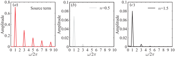
Figure 4: FFT analysis results showing active frequencies due to imposed frequency $\omega=2\pi$. (a) Resulting frequencies from FFT analysis applied directly to the source term of (72). (b,c) Resulting frequencies from FFT analysis applied on the numerical solution of (28) and corresponding to shear-thinning and shear-thickening fluids, respectively. Clearly, the source term itself predicts well the governing frequencies of the solution, though of course cannot predict the amplitudes.

In Figs. 4(b) and 4(c) we present the resulting frequencies of FFT analysis applied on the results of numerical simulations for shear-thinning and shear-thickening fluids, showing excellent agreement with the analytically predicted frequencies obtained from the first-order source term. From Figs. 4(b) and 4(c) we obtain that for actuation at the viscous-elastic time scale ($\omega\sim O(1)$), the dominant frequencies are

$$\omega_{a1}=\omega=2\pi,\quad\omega_{a2}=3\omega=3\cdot 2\pi,\quad\omega_{a3}=5\omega=5\cdot 2\pi,$$ (76)

and therefore the steady-state time variation of the pressure at any location $z$ can be approximately described by the superposition of only three sinusoidal waveforms

$$p(z,t)=A_{1}\left(z\right)\mathrm{e}^{i\omega_{\omega_{a1}}t}+A_{2}\left(z\right)\mathrm{e}^{i\omega_{\omega_{a2}}t}+A_{3}\left(z\right)\mathrm{e}^{i\omega_{\omega_{a3}}t}+\mathrm{c.c.},$$ (77)

where $A_{1}\left(z\right)$, $A_{2}\left(z\right)$ and $A_{3}\left(z\right)$ are complex functions solely depending on $z$ and ”c.c.” represents the complex conjugate of preceding terms.

Figure (5) summarizes the steady-state results of viscous-elastic interaction due to an oscillatory pressure (70). Figures 5(a,b,c) present the steady-state pressure distribution versus axial coordinate for one period of oscillations, obtained from numerical solution of (28) and corresponding to shear-thinning, Newtonian and shear-thickening fluids, respectively. Clearly, the shear-thinning fluid is characterized by the most rapid pressure decay rate similarly to the results in previous sections, thus suggesting the existence of a propagation front (which we however did not prove for this case).

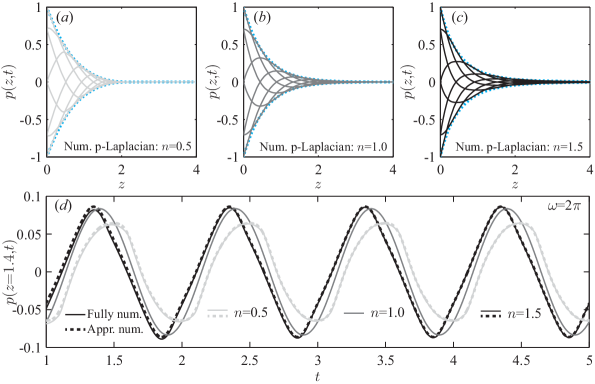
Figure 5: Numerical results showing the steady-state pressure distribution resulting from viscous-elastic interaction induced by oscillating inlet pressure with $\omega=2\pi$. (a,b,c) Pressure versus axial coordinate for one time period, corresponding to shear-thinning, Newtonian, and shear-thickening fluids, respectively. Dotted lines represent the envelope of the pressure decay, and indicate the most rapid decay for the shear-thinning fluid. (d) Comparison of numerical results (solid lines) and approximate solutions (dashed lines), (77), for pressure distributions at $z=1.4$ as a function of time and corresponding to $n=0.5,1,1.5$. While Newtonian fluid (dark gray line) is characterized by a sinusoidal waveform, shear-thinning (light gray lines) and shear-thickening (black lines) fluids exhibit non-sinusoidal ”saw-tooth” and ”shark-tooth” waveforms, respectively.

In Fig. 5(d), we compare the numerical solutions (solid lines) and approximate solutions (dashed lines), (77), for the pressure variation as a function of time at $z=1.4$, showing good agreement. As can be inferred from Fig. 5(d), in the steady-state the shear-thinning fluid exhibits a non-sinusoidal ”saw-tooth” waveform, whereas the shear-thickening is characterized by a non-sinusoidal ”shark-tooth” waveform.

V The inverse role of viscosity between viscous-elastic and Stokes’ problems

In Secs. IV B and IV C, we studied analytically and numerically the viscous-elastic interaction of power-law fluids through an elastic cylinder resulting from a constant or an oscillating pressure at the inlet. Specifically, we solved a homogeneous p-Laplacian equation that can be written in dimensional form as

$$\frac{\partial\tilde{p}}{\partial\tilde{t}}=\frac{n}{3n+1}\frac{\tilde{E}\tilde{h}_{m}\tilde{r}_{c}}{5-4\nu}\frac{\partial}{\partial\tilde{z}}\left(\frac{1}{\tilde{\eta}(\dot{\gamma})}\frac{\partial\tilde{p}}{\partial\tilde{z}}\right);\quad\tilde{\eta}(\dot{\gamma})=2^{\frac{1-n}{n}}\left(\frac{\tilde{\mu}_{eff}}{\tilde{r}_{c}}\right)^{\frac{1}{n}}\tilde{r}_{c}\left|\frac{\partial\tilde{p}}{\partial\tilde{z}}\right|^{\frac{n-1}{n}}.$$ (78)

We note that for $n=1$ (78) reduces to an unforced version of equation (2.53) derived by Elbaz and Gat Elbaz2014 .

This p-Laplacian equation is found in various fluid mechanics problems including Stokes’ first and second problems for power-law fluids, which involve the solution of the following p-Laplacian equation for $\tilde{u}_{z}$

$$\tilde{\rho}\frac{\partial\tilde{u}_{z}}{\partial\tilde{t}}=\frac{\partial}{\partial\tilde{z}}\left(\tilde{\eta}(\dot{\gamma})\frac{\partial\tilde{u}_{z}}{\partial\tilde{z}}\right);\quad\tilde{\eta}(\dot{\gamma})=\tilde{\mu}_{eff}\left|\frac{\partial\tilde{u}_{z}}{\partial\tilde{z}}\right|^{n-1},$$ (79)

subjected to a constant or an oscillatory velocity at $\tilde{z}=0$. The Stokes’ first problem was considered by Pascal Pascal1992 who showed that the velocity profile is compactly supported for shear-thickening fluids. Pritchard et al. Pritchard presented semi-analytical, self-similar and periodic solutions for the flow of a power-law fluid driven by a non-sinusoidal oscillating waveform at the wall and showed that in this case these solutions predict a finite penetration length $\tilde{l}_{p}$ for shear-thickening fluids, beyond which the fluid is essentially unaffected by external forcing and is motionless. To confirm these solutions, Pritchard et al. Pritchard studied numerically the Stokes’ second problem (on a finite numerical domain) with the sinusoidal boundary condition and the numerical results corresponding to shear-thickening fluids decay rapidly with the distance from the wall thus suggesting the existence of a finite penetration length. In addition, Pritchard et al. Pritchard obtained that the velocity of shear-thickening fluids adopt a ”saw-tooth” oscillating form, while shear-thinning fluids have a ”shark-tooth” oscillating form.

Clearly, the results we obtained in Secs. IV B and IV C are opposite to the results of Pascal Pascal1992 and Pritchard et al. Pritchard . To explain this difference we should examine the effect of viscosity in the p-Laplacian equations, (78) and (79), on the fluid penetration. While in Stokes’ equation, (79), viscosity contributes to diffusivity and thus to fluid penetration, in the viscous-elastic equation, (78), viscosity reduces the diffusivity and fluid penetration. This can be observed more clearly from the expressions of the penetration length, $\tilde{l}_{p}$, which can be obtained from scaling arguments as

$$\tilde{l}_{p,VE}\sim\sqrt{\tilde{E}\tilde{h}_{m}\tilde{r}_{c}\tilde{t}^{*}/\tilde{\eta}(\dot{\gamma})}\sim\sqrt{\tilde{E}\tilde{h}_{m}\tilde{t}^{*}}\frac{\left(\tilde{r}_{c}/\tilde{\mu}_{eff}\right)^{\frac{1}{2n}}}{\left|\partial\tilde{p}/\partial\tilde{z}\right|^{\frac{n-1}{2n}}},$$ (80)

$$\tilde{l}_{p,S}\sim\sqrt{\tilde{t}^{*}\tilde{\eta}(\dot{\gamma})/\tilde{\rho}}\sim\sqrt{\tilde{t}^{*}\tilde{\mu}_{eff}/\tilde{\rho}}\left|\frac{\partial\tilde{u}_{z}}{\partial\tilde{z}}\right|^{\frac{n-1}{2}},$$ (81)

where subscript VE indicates a viscous-elastic problem parameter, S indicates a Stokes’ problem parameter. Noting that for shear-thickening fluids ($n>1$), both viscosities (S) and (VE) tend to zero as the gradient of the velocity (or pressure) goes to zero, it follows from (80) and (81) that while for the Stokes’ problem the penetration length, $\tilde{l}_{p,S}$, goes to zero, for the viscous-elastic problem the penetration length tends to infinity, $\tilde{l}_{p,VE}\rightarrow\infty$, as $\tilde{\eta}(\dot{\gamma})\rightarrow 0$.

On the other hand, for shear-thinning fluids, both viscosities (S) and (VE) diverge as the gradient of the velocity (or pressure) goes to zero, and thus Stokes’ problem yields an infinite penetration length, $\tilde{l}_{p,S}\rightarrow\infty$, whereas the viscous-elastic problem exhibits a finite penetration length indicating the existence of the front in this case.

These conclusions are fully consistent with our results from Secs. IV B and IV C and with the results of Pascal Pascal1992 and Pritchard et al. Pritchard . Shear-thinning and shear-thickening fluids play opposite roles in the Stokes’ and the viscous-elastic problems.

VI Discussion and concluding remarks

In this work, we studied the viscous-elastic interaction and the flow of power-law fluids through an elastic cylinder. Applying the lubrication and the elastic shell approximations, we derived a p-Laplacian governing equation relating the fluidic pressure and the external forces acting on the cylinder. We showed that in this equation viscosity acts as an inverse diffusion coefficient, such that the familiar roles of shear-thinning and shear-thickening are inversed relative to similar equations that appear in Stokes’ problems. For example, for instantaneous mass injection and a step pressure applied at the inlet, our analysis revealed that a compactly supported propagation front exists solely for shear-thinning fluids, in contrast to Stokes’ problem where a compactly supported front is obtained for shear-thickening fluids. Furthermore, the scaling for penetration length, (80), based on a power-law viscosity model, further suggests that any Dirichlet-type boundary condition imposed at $z=0$, would result in compactly supported propagation for shear-thinning fluids, consistent with our numerical observations in Sec. IV C.

Throughout this work we have mainly considered the viscous-elastic dynamics due to imposed pressure at the inlet. However, we note that the solutions obtained in Sec. IV can be used to construct new solutions resulting from an external pressure distribution $p_{e}(z,t)$. Applying the Laplace transform on (28) we obtain that the solution for the pressure in Sec. IV A for impulse pressure applied at the inlet of a semi-infinite cylinder also holds for the case of a sudden localized pressure, $p_{e}=p_{e}H(t)\delta(z)$, applied to an infinitely long cylinder. Similarly, the solution for the pressure in the case of a discharging elastic tube ((65) with $\beta>0$, $p_{0}=0$) also holds for discharge due to suddenly applied constant pressure $p_{e}=p_{e}H(t)$. While the solutions for the pressure in these case are identical, the solutions for the corresponding deformation fields and the volume fluxes are different, and can be obtained from (26) and (54).

For weakly non-Newtonian fluids, we obtained the leading- and first-order asymptotic approximations, and showed (see Sec. IV C) that the source term in first-order equation, (35), is important as it enables physical insight on the non-Newtonian behavior without a direct solution.

The regime of an incompressible fluid with negligible inertia is commonly encountered in lab-on-chip and soft robotics applications. For the former, controlling the propagation of mass flux within microfluidic channels could be a mechanism the timing of simple delivery on chip, or controlling the extent of mixing between reagents. For soft robotics, control with non-Newtonian liquids holds to potential for additional degrees of freedom in modulation, and particularly with the use of compactly supported deformations where part of the structure can be guaranteed to stay stationary while another is translating. Furthermore, we believe that the dependence of the front on time and on specific value of $n$, can be used to indirectly measure the rheological properties of power-law shear-thinning liquids through measurements of deformation and front location.

References

- (1) C. Duprat and H. A. Stone (eds.), Fluid-Structure Interactions in Low-Reynolds-Number Flows, RSC Soft Matter Series (Royal Society of Chemistry, Cambridge, UK, 2016).
- (2) D. N. Ku, Blood flow in arteries, Annu. Rev. Fluid Mech. 29, 399 (1997).
- (3) W. Nichols, M. O’Rourke, and C. Vlachopoulos, McDonald’s blood flow in arteries:theoretical, experimental and clinical principles (CRC Press, 2011).
- (4) I. J. Hewitt, N. J. Balmforth, and J. R. De Bruyn, Elastic-plated gravity currents, Eur. J. Appl. Math. 26, 1 (2015).
- (5) D. Pihler-Puzovic, P. Illien, M. Heil, and A. Juel, Suppression of complex fingerlike patterns at the interface between air and a viscous fluid by elastic membranes, Phys. Rev. Lett. 108, 074502 (2012).
- (6) D. Pihler-Puzovic, R. Perillat, M. Russell, A. Juel, and M. Heil, Modelling the suppression of viscous fingering in elastic-walled Hele-Shaw cells, J. Fluid Mech. 731, 162 (2013).
- (7) T. T. Al-Housseiny, I. C. Christov, and H. A. Stone, Two-phase fluid displacement and interfacial instabilities under elastic membranes, Phys. Rev. Lett. 111, 034502 (2013).
- (8) D. Pihler-Puzovic, A. Juel, and M. Heil, The interaction between viscous fingering and wrinkling in elastic-walled Hele-Shaw cells, Phys. Fluids. 26, 022102 (2014).
- (9) D. Pihler-Puzovic, A. Juel, G. G. Peng, J. R. Lister, and M. Heil, Displacement flows under elastic membranes. Part 1. Experiments and direct numerical simulations, J. Fluid Mech. 784, 487 (2015).
- (10) G. G. Peng, D. Pihler-Puzovic, A. Juel, M. Heil, and J. R. Lister, Displacement flows under elastic membranes. Part 2. Analysis of interfacial effects., J. Fluid Mech. 784, 512 (2015).
- (11) A. E. Hosoi and L. Mahadevan, Peeling, healing, and bursting in a lubricated elastic sheet, Phys. Rev. Lett. 93, 137802 (2004).
- (12) J. R. Lister, G. G. Peng, and J. A. Neufeld, Viscous Control of Peeling an Elastic Sheet by Bending and Pulling, Phys. Rev. Lett. 111, 154501 (2013).
- (13) D. P. Holmes, B. Tavakol, G. Froehlicher, and H. A. Stone, Control and manipulation of microfluidic flow via elastic deformations, Soft Matter 9, 7049 (2013).
- (14) R. F. Shepherd, F. Ilievski, W. Choi, S. A. Morin, A. A. Stokes, A. D. Mazzeo, X. Chen, M. Wang, and G. M. Whitesides, Multigait soft robot, Proc. Natl Acad. Sci. 108, 20400 (2011).
- (15) R. V. Martinez, C. R. Fish, X. Chen, and G. M. Whitesides, Elastomeric origami: Programmable paper-elastomer composites as pneumatic actuators, Adv. Mater. 22, 1376 (2012).
- (16) A. D. Marchese, C. D. Onal, and D. Rus, Autonomous soft robotic fish capable of escape maneuvers using fluidic elastomer actuators, Soft Robotics 1, 75 (2014).
- (17) Y. Matia, T. Elimelech, and A. D. Gat, Leveraging nternal viscous flow to extend the capabilities of beam-shaped soft robotic actuators, Soft Robotics 4, 126 (2017).
- (18) S. Canic and A. Mikelic, Effective equations modeling the flow of a viscous incompressible fluid through a long elastic tube arising in the study of blood flow through small arteries, SIAM J. Appl. Dyn. Syst. 2, 431 (2003).
- (19) J. B. Grotberg and O. E. Jensen, Biofluid mechanics in flexible tubes, Annu. Rev. Fluid Mech. 36, 121 (2004).
- (20) M. Heil and A. L. Hazel, Fluid-structure interaction in internal physiological flows, Annu. Rev. Fluid Mech. 43, 141 (2011).
- (21) S. B. Elbaz and A. D. Gat, Dynamics of viscous liquid within a closed elastic cylinder subject to external forces with application to soft robotics, J. Fluid Mech. 758, 221 (2014).
- (22) B. S. Hardy, K. Uechi, J. Zhen, and H. P. Kavehpour, The deformation of flexible PDMS microchannels under a pressure driven flow, Lab on a Chip 9, 935 (2009).
- (23) J. M. de Rutte, K. G. H. Janssen, N. R. Tas, J. C. T. Eijkel, and S. Pennathur, Numerical investigation of micro-and nanochannel deformation due to discontinuous electroosmotic flow, Microfluid Nanofluid 20, 150 (2016).
- (24) H. Pascal, Similarity solutions to some unsteady flows of non-Newtonian fluids of power-law behavior, Intl J. Non-Linear Mech. 27, 759 (1992).
- (25) L. Ai and K. Vafai, An investigation of Stokes’ second problem for non-Newtonian fluids, Numer. Heat Tr. A-Appl. 47, 955 (2005).
- (26) D. Pritchard, C. R. McArdle, and S. K. Wilson, The Stokes boundary layer for a power-law fluid, J. Non-Newtonian Fluid Mech. 166, 745 (2011).
- (27) R. B. Bird, R. C. Armstrong, and O. Hassager, Dynamics of polymeric liquids. Volume 1: Fluid Mechanics (2nd ed. John Wiley and Sons, 1987).
- (28) S. Timoshenko and J. N. Goodier, Theory of elasticity (McGraw-Hill, New York, 1951).
- (29) P. Howell, G. Kozyreff, and J. Ockendon, Applied solid mechanics (Cambridge University Press, 2009).
- (30) See Supplemental Material for additional details.
- (31) H. Pascal, and F. Pascal, Flow of non-Newtonian fluid through porous media, Intl J. Engng Sci. 23, 571 (1985).
- (32) H. Pascal, On propagation of pressure disturbances in a non-Newtonian fluid flowing through a porous medium, Intl J. Non-Linear Mech. 26, 475 (1991).
- (33) V. Di Federico and V. Ciriello, Generalized solution for 1-d non-Newtonian flow in a porous domain due to an instantaneous mass injection, Transp. Porous Med. 93, 63 (2012).
- (34) B. R. Duffy, D. Pritchard and S. K. Wilson, The shear-driven Rayleigh problem for generalised Newtonian fluids, J. Non-Newtonian Fluid Mech. 206, 11 (2014).
- (35) A. B. Ross, S. K. Wilson, and B. R. Duffy, Blade coating of a power-law fluid, Phys. Fluids. 11, 958 (1999).
- (36) Q. Cheng, Z. Sun, G. A. Meininger, and M. Almasri, Note: Mechanical study of micromachined polydimethylsiloxane elastic microposts, Rev. Sci. Instrum. 81, 106104 (2010).
- (37) S. Longo, V. Di Federico, and V. Chiapponi, A dipole solution for power-law gravity currents in porous formations, J. Fluid Mech. 778, 534 (2015).
- (38) M. Abramowitz and I. A. Stegun, Handbook of Mathematical Functions (Dover, 1964).
- (39) L. J. Slater, Generalized hypergeometric functions (Cambridge University Press, 1966).