Finite Dissipation in Anisotropic Magnetohydrodynamic Turbulence

Abstract

In presence of an externally supported, mean magnetic field a turbulent, conducting medium, such as plasma, becomes anisotropic. This mean magnetic field, which is separate from the fluctuating, turbulent part of the magnetic field, has considerable effects on the dynamics of the system. In this paper, we examine the dissipation rates for decaying incompressible magnetohydrodynamic (MHD) turbulence with increasing Reynolds number, and in the presence of a mean magnetic field of varying strength. Proceeding numerically, we find that as the Reynolds number increases, the dissipation rate asymptotes to a finite value for each magnetic field strength, confirming the Kármán-Howarth hypothesis as applied to MHD. The asymptotic value of the dimensionless dissipation rate is initially suppressed from the zero-mean-field value by the mean magnetic field but then approaches a constant value for higher values of the mean field strength. Additionally, for comparison, we perform a set of two-dimensional (2DMHD) and a set of reduced MHD (RMHD) simulations. We find that the RMHD results lie very close to the values corresponding to the high mean-field limit of the three-dimensional runs while the 2DMHD results admit distinct values far from both the zero mean field cases and the high mean field limit of the three-dimensional cases. These findings provide firm underpinnings for numerous applications in space and astrophysics wherein von Kármán decay of turbulence is assumed.

I Introduction and Background

Turbulence is a ubiquitous, although incompletely understood phenomena. In turbulent astrophysical plasmas, velocity and magnetic fields are often equally important, and magnetohydrodynamic (MHD) turbulence, the case considered here, becomes an appropriate description. Energy supply for turbulence usually originates at large scales due to some type of stirring or driving mechanism, after which the energy cascades to smaller scales, finally reaching the dissipation scale where the energy is dissipated into heat by viscosity and resistivity. For incompressible hydrodynamics, the single scalar viscosity $\nu$ parameterizes microscopic nonideal effects, such that, for laminar flows the energy dissipation rate vanishes when $\nu\to 0$. However, for turbulent flows, following the hypothesis stated by Taylor Taylor (1935) and von Kármán & Howarth  de Kármán and Howarth (1938) and later employed by Kolmogorov Kolmogorov (1941a), in the zero viscosity, infinite Reynolds number $Re\sim 1/\nu\to\infty$ limit, the energy dissipation rate approaches a constant, nonzero limitDonzis et al. (2005). (The renowned Kolmogorov theory of universal scaling in the inertial range (K41) Kolmogorov (1941b), in essence assumes this limiting behavior.) This so-called “dissipative anomaly” is well supported in experiments and computations Ravelet et al. (2008); Saint-Michel et al. (2014).

For the case of incompressible MHD, there are two relevant dissipation coefficients, viscosity $(\nu)$ and resistivity $(\mu)$, associated with velocity and magnetic field, respectively. The limit of zero viscosity and resistivity $(\nu,\mu\rightarrow 0)$ is again of interest with regard to fully developed turbulent systems. In practice one finds that, for essentially all astrophysical as well as terrestrial turbulent systems, the mechanical and magnetic Reynolds numbers (inverse of viscosity and resistivity in non-dimensional units) are of large, and sometimes colossal magnitude, justifying the success of turbulence phenomenologies like K41. For example, the effective mechanical and magnetic Reynolds number, in the solar wind, are of the order of $10^{5}$ or more Matthaeus et al. (2005) (also see Verma (1996)), and much larger in the interstellar medium. Therefore, one might be tempted to assume $\nu,\mu=0$ as an approximation. However, in analogy to the hydrodynamics case, the limit $\nu,\mu\rightarrow 0$ is very different from the $\nu,\mu=0$ case. This is manifested in the counterintuitive phenomena that as the limit $\nu,\mu\rightarrow 0$ is approached, the total turbulent energy dissipation rate does not vanish, but remains finite. MHD energy dissipation is exactly zero for the ideal case $(\nu,\mu=0)$. Onsager Onsager (1949) conjectured that this problem of energy-dissipation anomaly arises due to lack of smoothness in the velocity field increments in the context of three-dimensional hydrodynamic turbulence. Based on this idea of lack of smoothness in the velocity field, Duchon $\&$ Robert Duchon and Robert (2000) derived a local form of dissipation which was generalized to incompressible Hall MHD by Galtier Galtier (2018). An apparent explanation of anomalous dissipation was given in a work by Cichowlas et al. Cichowlas et al. (2005) who showed that even for ideal Eulerian flows, the large-wavenumber modes play the role of an effective eddy viscosity leading to an approximate Kolmogorov scaling at the inertial scales. This idea was further extended to two-dimensional MHD by Krstulovic et al. Krstulovic et al. (2011). Here we will examine this apparently singular behavior (see e.g., Morf et al. (1980); Kerr (1993); Dmitruk and Montgomery (2005); Mininni and Pouquet (2009)) not from a rigorous mathematical perspective, but from an empirical perspective based on accurate spectral method computations.

Taylor first suggested, based on empirical arguments, that the dissipation rate in a fully developed turbulent system becomes independent of viscosity. Kármán and Howarth de Kármán and Howarth (1938) established Taylor’s results more rigorously, assuming that the shape of the two-point correlation function remains unchanged. The first experimental verification of Kármán and Howarth’s result came from an experiment performed by Batchelor and Townsend Batchelor (1953); Batchelor and Townsend (1947, 1948a, 1948b) using wind tunnel measurements. Politano and Pouquet Politano and Pouquet (1998) generalized the von Kármán-Howarth equations for isotropic MHD. Wan et al. Wan et al. (2012) investigated nonuniversality of Kármán-Howarth like decay in MHD in the presence of factors like mean magnetic field, helicity, etc.

Recently, Wu et al. Wu et al. (2013) and Parashar et al. Parashar et al. (2015) have shown using particle in cell (PIC) simulations that even in the case of weakly collisional plasmas, the von Kármán decay law remains valid. Most of these studies were interested in the temporal behavior of the fluctuation amplitude and its relationship with the large-scale fluctuations and an energy-containing length scale. For neutral fluids, the variation of dimensionless dissipation rate, $C_{\epsilon}$ with Reynolds number was studied experimentally in shear flows  Pearson et al. (2002), numerically in homogeneous incompressible flows Kaneda et al. (2003), and in weakly compressible flows Pearson et al. (2004). In all cases, an asymptotic value of $C_{\epsilon}\approx 0.5$ was found. We remark here that the dimensionless dissipation rate, $C_{\epsilon}$, as defined in Pearson et al. Pearson et al. (2004) is proportional to one of the constants in von Kármán decay phenomenology (See Appendix B of  Usmanov et al. (2014)). Mininni and Pouquet Mininni and Pouquet (2009) carried out direct numerical simulations (DNS) of decaying isotropic MHD turbulence, demonstrating that the mean dissipation rate per unit mass, $\epsilon$, remains finite and becomes independent of viscosity and resistivity as the Reynolds number (Taylor-scale Reynolds number, $R_{\lambda}$, in this case) increases. Dallas and Alexakis Dallas and Alexakis (2014) performed a similar analysis showing the variation of dimensionless dissipation rate with Taylor-scale Reynolds number with initial velocity and current density being highly correlated. A comparison with Mininni and Pouquet (2009) revealed that the dimensionless dissipation rate saturates to a finite value but the level of saturation depends on the strength of initial cross-correlation. Recently, Linkmann et al. Linkmann et al. (2015, 2017) have performed a series of investigations for similar analysis in isotropic MHD. By fitting a model equation, an asymptotic value of dimensionless dissipation rate, $C_{\epsilon,\infty}=0.265\pm 0.013$, was found for nonhelical decaying MHD with no mean field. This value is considerably different from the fluid case. McComb et al. McComb and Fairhurst (2017) derived a similar model equation for fluid turbulence.

The presence of a mean magnetic field suppresses the decay rate in MHD systems and renders the system anisotropic. Early studies by Hossain et al. Hossain et al. (1995, 1996) at low Reynolds number demonstrated that the mean field initially inhibits dissipation, but the effect of Alfvénic propagation soon saturates for sufficiently large values of the mean field. More recently, Bigot et al. Bigot et al. (2008a, b); Bigot and Galtier (2011) investigated the energy decay in the presence of a strong uniform magnetic field. Zhdankin et al. Zhdankin et al. (2017) also studied the effect of a mean field at dissipation sites in MHD turbulence. Naturally, one would expect a decrease of the dimensionless dissipation rate (or, the von Kármán decay constant) with increasing strength of mean field. We present here a further analysis of the dissipation rate for increasing values of mean field. We find that for each value of the mean field, the dissipation rate asymptotes to a finite value in the limit of large Reynolds number. These results are relevant for systems in which the anisotropy due to presence of a mean magnetic field cannot be neglected. Such situations are often realized in astrophysical plasmas near stellar objects. Our results show that the value of the dimensionless dissipation rate is well separated from the isotropic value for a strong mean field. We first reestablish the isotropic case by comparing with results from Linkmann et al. (2017) and then proceed in similar fashion to anisotropic cases.

II Equations and Approach

The equations of three dimensional incompressible MHD, in the absence of external forcing, are written as,

$$\frac{\partial\mathbf{u}}{\partial t}+(\mathbf{u}\cdot\mathbf{\nabla})\mathbf{u} = -\mathbf{\nabla}P+(\mathbf{j}\times\mathbf{B})+\nu\mathbf{\nabla}^{2}\mathbf{u},$$ (1)

$$\frac{\partial\mathbf{B}}{\partial t}+(\mathbf{u}\cdot\mathbf{\nabla})\mathbf{B} = (\mathbf{B}\cdot\mathbf{\nabla})\mathbf{u}+\mu\mathbf{\nabla}^{2}\mathbf{B},$$ (2)

$$\mathbf{\nabla}\cdot\mathbf{u} = 0,$$ (3)

$$\mathbf{\nabla}\cdot\mathbf{B} = 0,$$ (4)

where $\mathbf{u}$ is the fluctuating velocity field, $\mathbf{B}$ is the total magnetic field which we assume can be decomposed into a spatially uniform mean and a fluctuating part, $\mathbf{B}(\mathbf{r},t)=\mathbf{B_{0}}+\mathbf{b}(\mathbf{r},t)$. Without any loss of generality, we choose $\mathbf{B_{0}}=B_{0}\mathbf{\hat{z}}$. $P$ is the total (thermal+magnetic) pressure field, $\mathbf{j}=(\mathbf{\nabla}\times\mathbf{B})/\mu_{0}$ is the current density, $\nu$ is the kinematic viscosity, and $\mu$ is the magnetic diffusivity. Eq. (3) enforces incompressibility. For simplicity, we assume the fluid density $\rho$ is constant and set it to unity. For this study, we consider unit magnetic Prandtl number $(\mathrm{Pm}=\nu/\mu)$, i.e., equal viscosity and resistivity,

$$\nu=\mu.$$ (5)

With this constraint, the MHD equations Eqs. (1)–(4) can be written in terms of the Elsasser variables, $\mathbf{z_{\pm}}=\mathbf{u}\pm\mathbf{b}$, as,

$$\frac{\partial\mathbf{z}_{\pm}}{\partial t}=\pm\mathbf{v_{A}}\cdot\mathbf{\nabla}\mathbf{z}_{\pm}-\mathbf{z}_{\mp}\cdot\mathbf{\nabla}\mathbf{z}_{\pm}-\mathbf{\nabla}P+\nu\mathbf{\nabla}^{2}\mathbf{z}_{\pm}.$$ (6)

Here, $\mathbf{v_{A}}$ is the Alfvén velocity defined as $\mathbf{v_{A}}=\mathbf{B_{0}}/\sqrt{4\pi}$. The Elsasser energies are given by

$$Z^{2}_{\pm}=\langle|\mathbf{z}_{\pm}|^{2}\rangle=\langle|\mathbf{u}\pm\mathbf{b}|^{2}\rangle.$$ (7)

Following the argument associated with preservation of the functional form of the two-point correlation functions, one can generalize the von Kármán-Howarth de Kármán and Howarth (1938) result to isotropic MHD Politano and Pouquet (1998) or MHD isotropic in a plane perpendicular to a strong mean field Wan et al. (2012),

$$\frac{dZ^{2}_{\pm}}{dt} = -\alpha_{\pm}\frac{Z^{2}_{\pm}Z_{\mp}}{L_{\pm}},$$ (8)

$$\frac{dL_{\pm}}{dt} = \beta_{\pm}Z_{\mp},$$ (9)

where $\alpha_{\pm}$ and $\beta_{\pm}$ are constants, and $L_{\pm}$ are the energy-containing scales corresponding to the two Elsasser variables. Precise definitions of $L_{\pm}$ depend on the phenomenology used. We shall come back to the definition of energy-containing scale later in the paper. For small cross helicity $(H_{c}\simeq 0)$, the $``+"$ and $``-"$ variables remain almost equal, so that one can write,

$$\frac{dZ^{2}}{dt} = -\alpha\frac{Z^{3}}{L},$$ (10)

$$\frac{dL}{dt} = \beta Z,$$ (11)

where, $Z\simeq Z_{+}\simeq Z_{-}$. It is apparent from these equations that the sequence of assumptions (especially, self-preservation of the correlations) leading to this point implies that the energy dissipation rate becomes independent of the dissipation coefficients $\nu=\mu$. It is one of the main goals of this paper to measure the finite energy dissipation rate in the asymptotic limit of large Reynolds number for MHD in presence of a mean field at zero magnetic and cross helicity.

The mean turbulent energy dissipation rate per unit mass in incompressible MHD, for unit magnetic Prandtl number $(\mathrm{Pm})$, can be written as,

$$\epsilon(t)=\nu\langle\omega^{2}+j^{2}\rangle,$$ (12)

where $\mathbf{\omega}=\mathbf{\nabla}\times\mathbf{u}$ is the vorticity and $\langle\cdots\rangle$ denotes spatial averaging.

Linkmann et al. Linkmann et al. (2015, 2017) proposed a definition of the non-dimensional energy dissipation rate in MHD turbulence as,

$$C_{\epsilon}(t) = C^{+}_{\epsilon}(t)+C^{-}_{\epsilon}(t),$$ (13)

where

$$C^{\pm}_{\epsilon}(t) = \frac{\epsilon(t)L_{\pm}(t)}{W_{\pm}(t)^{2}W_{\mp}(t)},$$ (14)

where

$$L_{\pm}(t)=\frac{3\pi}{8E_{\pm}(t)}\int k^{-1}\langle|\mathbf{z}_{\pm}(\mathbf{k},t)|^{2}\rangle d\mathbf{k},$$ (15)

where $\mathbf{z}_{\pm}(\mathbf{k},t)$ denotes the Fourier transform of the respective Elsasser variables. Assuming isotropy, the rms values of the Cartesian components of $Z_{\pm}^{2}$ are given by,

$$W^{2}_{\pm}=Z^{2}_{\pm}/3.$$ (16)

The $W_{\pm}$ are the Elsasser variable analogs of the $u^{\prime}$ in $E^{u}=3(u^{\prime})^{2}/2$, which is the classical definition often employed in isotropic hydrodynamic work Batchelor (1953). Here we use

$$E_{\pm}(t)=2E(t)\pm 2H_{c}(t)\equiv Z^{2}_{\pm},$$ (17)

where $E(t)$ is the total energy

$$E(t)=\frac{1}{4}\int\langle|\mathbf{z}_{+}(\mathbf{k},t)|^{2}+|\mathbf{z}_{-}(\mathbf{k},t)|^{2}\rangle d\mathbf{k},$$ (18)

and $H_{c}(t)$ is the cross helicity

$$H_{c}(t)=\frac{1}{4}\int\langle|\mathbf{z}_{+}(\mathbf{k},t)|^{2}-|\mathbf{z}_{-}(\mathbf{k},t)|^{2}\rangle d\mathbf{k}.$$ (19)

For $H_{c}\simeq 0$, one expects $C^{+}_{\epsilon}\simeq C^{-}_{\epsilon}$. Further, Linkmann et al. Linkmann et al. (2015, 2017) also suggested a generalized Reynolds number defined as

$$R_{-} = \frac{W_{-}L_{+}}{(\nu+\mu)},$$ (20)

In this paper we have studied the variation of dimensionless dissipation rate, as defined by Eqs. (13)–(14) with generalized Reynolds number defined in Eq. (20). For comparison, we also report the integral scale Reynolds number defined as

$$R_{L} = \frac{u^{\prime}L_{\mathrm{int}}}{\nu},$$ (21)

where

$$L_{\mathrm{int}}=\bigg{(}\frac{3\pi}{4}\bigg{)}\frac{\int k^{-1}E^{u}(k)dk}{\int E^{u}(k)dk}.$$ (22)

and $u^{\prime}$ denotes the rms speed with $E^{u}=3(u^{\prime})^{2}/2$. Here $E^{u}(k)$ denotes the omnidirectional kinetic energy spectrum and $E^{u}=\int E^{u}(k)dk$ is the total kinetic energy. Similarly, the Taylor microscale Reynolds number is defined as

$$R_{\lambda} = \frac{u^{\prime}\lambda}{\nu},$$ (23)

where

$$\lambda=\bigg{[}\frac{5\int E^{u}(k)dk}{\int k^{2}E^{u}(k)dk}\bigg{]}^{1/2}=u^{\prime}\sqrt{\frac{15\nu}{\epsilon}}.$$ (24)

The effect of a mean magnetic field on magnetohydrodynamic turbulence was first investigated and quantified by Shebalin et al. Shebalin et al. (1983) in two dimensions, and generalized to three dimensions by Oughton et al. Oughton et al. (1994). Spectral anisotropy in three dimensions is quantified by defining Shebalin angles, $\theta_{Q}$ as

$$\tan^{2}\theta_{Q}(t)=\frac{\sum k^{2}_{\perp}|\mathbf{Q}(\mathbf{k},t)|^{2}}{\sum k^{2}_{\parallel}|\mathbf{Q}(\mathbf{k},t)|^{2}},$$ (25)

where $k_{\parallel}$ is the wave vector component along the direction of the mean magnetic field, $k_{\perp}$ is the wave vector in the plane perpendicular to the mean field, and the summations extend over all values of wave vector $\mathbf{k}$. In the present notation, $k_{\parallel}=k_{z}$ and $k^{2}_{\perp}=k^{2}_{x}+k^{2}_{y}$. In general $\mathbf{Q}$ can be any vector field, although here we consider only velocity field $\mathbf{u}$, and magnetic field $\mathbf{b}$.

We define

$$r=\frac{2E^{b}}{B^{2}_{0}},$$ (26)

where $E^{b}=\delta b^{2}/2$ is the total magnetic field fluctuation energy. Therefore, $\sqrt{r}$ is the ratio of fluctuation amplitude and mean magnetic field strength.

$$r=\bigg{(}\frac{\delta b}{B_{0}}\bigg{)}^{2}.$$ (27)

III Numerical Method

We solve the MHD equations in a periodic box of dimension $(2\pi)^{3}$ using a pseudo-spectral method in a Fourier basis. We employ second-order Runge-Kutta (RK2) scheme for time advancement and the $2/3$ rule for dealiasing. Instead of using an automatically adjustable time step, in this study the time step was held constant for a set of runs, but halved when instabilities occurred. All the runs have been initialized with a modal spectrum proportional to $1/[1+(k/k_{0})^{11/3}]$, where the “knee” of the spectrum is $k_{0}=4$, and only Fourier modes within the band $1\leq k\leq 15$ are excited. The total kinetic and magnetic energy are both normalized to 0.5 initially. All the measurements have been made at the time of highest dissipation. In all runs, the kinetic, magnetic, and cross helicities are small initially and remain so during the simulation times considered. Further, since velocity and magnetic fields are generated independently, we may assume that cross correlations involving higher derivatives Dallas and Alexakis (2014) are suitably small throughout.

In all runs, the maximum resolved wavenumber, $k_{\mathrm{max}}$, is greater than the dissipation wavenumber (reciprocal of the Kolmogorov length scale $\eta$) defined as

$$k_{\mathrm{diss}}=\frac{1}{\eta}=\bigg{(}\frac{\epsilon}{\nu^{3}}\bigg{)}^{1/4}.$$ (28)

Wan et al. Wan et al. (2010) showed that the ratio $k_{\mathrm{max}}/k_{\mathrm{diss}}=k_{\mathrm{max}}\eta$ should be at least three for sufficient numerical accuracy of fourth-order moments. However, for studies of the present kind, as was earlier reported by Pearson et al. Pearson et al. (2004), we find that $k_{\mathrm{max}}\eta\geq 1$ suffices and increasing resolution further does not substantially change the results. Recall that the more strict requirement proposed by Wan et al Wan et al. (2010) pertains mainly to higher-order statistics and coherent structures, while accurate portrayal of lower-order quantities such as energy spectra, which control instantaneous dissipation, have less stringent requirements. This can also be seen from Table II of  Wan et al. (2010) where $k_{\mathrm{diss}}$ becomes accurate in the range $1\leq k_{\mathrm{max}}\eta\leq 1.9$. Since $k^{4}_{\mathrm{diss}}=\epsilon/\nu^{3}$, this implies that dissipation rate also becomes accurate in this range.

The details of the simulations used in this study are found in Table 1.

Table 1: Parameters for three dimensional spectral simulations: Mean magnetic field strength $B_{0}$, grid resolution $N^{3}$, viscosity and resistivity $\nu$ and $\mu$ (set equal), Taylor scale Reyolds number $R_{\lambda}$, Integral scale Reynolds number $R_{L}$, Generalized Reynolds number $R_{-}$, Dimensionless dissipation rate $C_{\epsilon}$, Shebalin angles for velocity field $\theta_{u}$, and for magnetic field $\theta_{b}$, Square of ratio of fluctuation amplitude and mean magnetic field $r=(\delta b/B_{0})^{2}$ (Not Applicable for $B_{0}=0$ case), time step $dt$, Ratio of maximum resolved wavenumber and dissipation wavenumber $k_{\mathrm{max}}\eta$. See text for definitions of the quantities. All measurements have been made near the time of maximum dissipation.

$B_{0}$	$N^{3}$	$\nu=\mu$	$R_{\lambda}$	$R_{L}$	$R_{-}$	$C_{\epsilon}$	$\theta_{u}$	$\theta_{b}$	$r$	$dt$	$k_{\mathrm{max}}\eta$
		$(\times 10^{-3})$								$(\times 10^{-4})$
$0$	$256^{3}$	$2.0$	$32.53$	$116.09$	$89.05$	$0.456$	54.7	54.8	NA	$10.0$	$1.83$
$0$	$512^{3}$	$1.0$	$48.07$	$216.26$	$166.82$	$0.382$	54.7	54.6	NA	$5.0$	$2.24$
$0$	$512^{3}$	$0.5$	$68.44$	$394.21$	$308.21$	$0.330$	54.8	54.7	NA	$5.0$	$1.36$
$0$	$768^{3}$	$0.4$	$76.06$	$483.43$	$382.76$	$0.316$	54.6	54.4	NA	$4.0$	$1.73$
$0$	$768^{3}$	$0.3$	$87.68$	$622.84$	$496.21$	$0.300$	54.6	54.5	NA	$4.0$	$1.40$
$0$	$1024^{3}$	$0.2$	$105.7$	$886.04$	$713.61$	$0.285$	54.9	55.0	NA	$2.5$	$1.39$
$0$	$1536^{3}$	$0.15$	$121.68$	$1126.96$	$910.97$	$0.270$	54.7	54.6	NA	$1.5$	$1.69$
$0$	$2048^{3}$	$0.1$	$145.63$	$1605.56$	$1313.66$	$0.261$	54.6	54.7	NA	$1.25$	$1.66$
$1$	$256^{3}$	$2.0$	$40.59$	$121.5$	$88.59$	$0.356$	60.2	61.8	0.7550	$10$	$1.92$
$1$	$512^{3}$	$1.0$	$59.94$	$228.62$	$168.50$	$0.298$	62.8	63.9	0.7377	$5.0$	$2.36$
$1$	$512^{3}$	$0.5$	$86.22$	$413.14$	$303.21$	$0.264$	64.9	65.7	0.7209	$5.0$	$1.43$
$1$	$768^{3}$	$0.4$	$96.17$	$506.29$	$374.40$	$0.254$	58.0	59.9	0.7138	$4.0$	$1.82$
$1$	$768^{3}$	$0.3$	$110.80$	$656.66$	$485.14$	$0.249$	66.1	66.8	0.7074	$4.0$	$1.47$
$1$	$1024^{3}$	$0.2$	$135.28$	$931.42$	$688.66$	$0.236$	66.6	67.1	0.7029	$2.5$	$1.45$
$1$	$1536^{3}$	$0.15$	$159.67$	$1273.54$	$932.60$	$0.238$	67.3	67.6	0.7060	$2.0$	$1.77$
$1$	$2048^{3}$	$0.1$	$190.99$	$1811.17$	$1331.78$	$0.234$	67.0	67.3	0.6986	$1.25$	$1.73$
$3$	$256^{3}$	$2.0$	$59.15$	$137.51$	$96.14$	$0.216$	64.6	65.3	0.0953	$2.5$	$2.18$
$3$	$512^{3}$	$1.0$	$90.3$	$256.40$	$183.8$	$0.160$	69.8	70.3	0.0899	$1.0$	$2.77$
$3$	$512^{3}$	$0.5$	$134.42$	$463.69$	$331.23$	$0.132$	74.0	74.5	0.0870	$1.0$	$1.72$
$3$	$512^{3}$	$0.4$	$157.05$	$572.75$	$408.17$	$0.120$	75.1	75.5	0.0882	$1.0$	$1.48$
$3$	$768^{3}$	$0.3$	$177.78$	$738.42$	$524.07$	$0.122$	76.7	77.2	0.0871	$9.0$	$1.77$
$3$	$1024^{3}$	$0.2$	$216.76$	$1054.46$	$752.93$	$0.116$	78.2	78.6	0.0846	$0.8$	$1.77$
$3$	$1024^{3}$	$0.15$	$247.75$	$1367.76$	$977.78$	$0.114$	79.1	79.4	0.0839	$0.8$	$1.42$
$3$	$1536^{3}$	$0.1$	$299.74$	$1961.17$	$1406.34$	$0.111$	80.0	80.3	0.0838	$0.5$	$1.57$
$8$	$256^{3}$	$2.0$	$67.45$	$141.86$	$99.52$	$0.169$	63.2	63.5	0.013	$1.0$	$2.35$
$8$	$512^{3}$	$1.0$	$98.98$	$247.13$	$176.00$	$0.131$	69.3	69.7	0.0125	$0.5$	$2.96$
$8$	$512^{3}$	$0.5$	$159.41$	$459.39$	$327.15$	$0.094$	73.8	74.0	0.0124	$0.5$	$1.86$
$8$	$512^{3}$	$0.4$	$190.30$	$572.86$	$407.77$	$0.082$	74.8	75.0	0.0126	$0.5$	$1.61$
$8$	$512^{3}$	$0.3$	$225.92$	$725.48$	$514.83$	$0.074$	76.6	76.7	0.0124	$0.5$	$1.33$
$8$	$768^{3}$	$0.2$	$284.55$	$1014.84$	$726.54$	$0.064$	78.3	78.4	0.0123	$0.3$	$1.49$
$15$	$256^{3}$	$2.0$	$66.5$	$138.08$	$96.15$	$0.173$	63.7	64.0	0.0037	$0.65$	$2.34$
$15$	$512^{3}$	$1.0$	$101.34$	$249.22$	$178.09$	$0.125$	69.6	69.8	0.0036	$0.3$	$2.99$
$15$	$512^{3}$	$0.5$	$163.05$	$461.06$	$327.82$	$0.090$	73.9	74.3	0.0036	$0.3$	$1.88$
$15$	$512^{3}$	$0.4$	$184.57$	$556.69$	$397.84$	$0.084$	74.8	74.9	0.0035	$0.3$	$1.61$
$15$	$512^{3}$	$0.3$	$228.77$	$727.64$	$519.81$	$0.072$	76.4	76.6	0.0035	$0.3$	$1.33$
$15$	$768^{3}$	$0.2$	$292.14$	$1023.87$	$730.58$	$0.062$	78.4	78.4	0.0035	$0.25$	$1.51$

Measurements are made at instant of peak dissipation, and shortly after this time the simulations are stopped. Ideally, one should consider performing an ensemble of runs and then calculate the statistics. However, the computational cost being prohibitively expensive, particularly for the high mean field cases, we defer such refinements to a later time.

IV Results

The dimensionless dissipation rates, obtained from the runs in Table 1, are plotted as function of the generalized Reynolds number in Fig. 1.

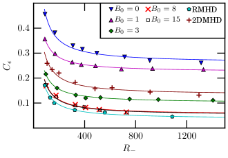
Figure 1: Dimensionless dissipation rate $(C_{\epsilon})$ plotted as a function of generalized Reynolds number $R_{-}$ for three-dimensional runs with different values of mean field $B_{0}$, one set of two-dimensional runs, and one set of reduced MHD runs along with fitted polynomials represented by continuous lines of same color as the corresponding runs.

Linkmann et al. Linkmann et al. (2015, 2017) showed that for isotropic MHD one can fit a simple model equation to $C_{\epsilon}$, provided $R_{-}\geq 80$,

$$C_{\epsilon}=C_{\epsilon,\infty}+\frac{A}{R_{-}}+O(R^{-2}_{-}),$$ (29)

where $C_{\epsilon,\infty}$ is the asymptotic value of $C_{\epsilon}$ as $R_{-}$ tends to $\infty$, $A$ is a time dependent coefficient, and $O(R^{-2}_{-})$ represents terms of higher order, which we are neglecting here. For lower Reynolds numbers, second order and higher terms cannot be neglected and may be important to derive model equations such as those described in  Linkmann et al. (2015, 2017). Since the main goal of this paper is not to build such model equations, but to measure the asymptotic value of the dimensionless dissipation rate and investigate its variation with mean magnetic field, we consider only high Reynolds numbers $(R_{-}\geq 80)$ and work only with the leading-order term.

We fit Eq. (29) to each set of runs; see Table 1. The solid lines in Fig. 1 are obtained from this fitting. We use a least-square fitting technique to fit the polynomial Eq. (29) to the data for each value of the mean magnetic field, which ranges over values $0,1,3,8,$ and $15$. In all cases we see that the fits agree reasonably well with the the sets of individual data points, and in some cases the agreement is excellent. The asymptotic values, i.e., the values of $C_{\epsilon,\infty}$, obtained by this procedure, are reported in Table 2.

Table 2: Summary of the asymptotic non-dimensional dissipation rate $C_{\epsilon,\infty}$ from different simulation sets of Table 1, and sets of RMHD and 2DMHD runs. Additionally, we report the value of the constant $A$ in Eq. (29).

$B_{0}$	$C_{\epsilon,\infty}$	$A$
$0.0$	$0.260\pm 0.007$	$18\pm 1$
$1.0$	$0.224\pm 0.002$	$11.8\pm 0.4$
$3.0$	$0.100\pm 0.002$	$11.0\pm 0.5$
$8.0$	$0.053\pm 0.006$	$12\pm 1$
$15.0$	$0.051\pm 0.005$	$12.1\pm 0.9$
RMHD	$0.036\pm 0.005$	$11.5\pm 0.8$
2DMHD	$0.132\pm 0.007$	$14\pm 1$

The value for the isotropic case is in agreement with the one reported in Linkmann et al. (2017), within uncertainty. The values of $C_{\epsilon,\infty}$ for $B_{0}>0$ decrease first with increasing strength of the mean field, but then saturate. This can be seen by comparing the two sets of data obtained for $B_{0}=8.0$ and $B_{0}=15.0$, which almost lie on top of each other. Quantitatively, it can be seen from Table 2 that the two values of $C_{\epsilon}$ for the $B_{0}=8.0$ and $B_{0}=15.0$ case lie within their limits of simulation uncertainty. This result is reminiscent of the Hossain et al. Hossain et al. (1996) study, that observed a suppression of dissipation rate due to a mean field of moderate strength compared to the dissipation rate in the isotropic case. This effect, however, saturates at higher mean field strengths. This is explained by noticing that the mean magnetic field suppresses spectral transfer parallel to the mean field, so that the spectrum becomes progressively more anisotropic, saturating at an anisotropy determined by the parallel bandwidth of the initial data (or forcing) Shebalin et al. (1983); Oughton et al. (1994); Bigot and Galtier (2011). Once saturated, further increase of the mean field has negligible effect. Thus, at strong mean field values, the Alfvén time does not play a dominant role in determining the triple decorrelation time that establishes the spectral transfer rates (see e.g., Zhou et al. (2004)).

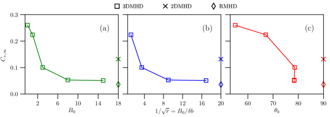
Figure 2: Asymptotic value of the dimensionless dissipation rate $C_{\epsilon}$ plotted against different measures of anisotropy. Panel (a): $C_{\epsilon,\infty}$ versus mean magnetic field strength $B_{0}$, panel (b): $C_{\epsilon,\infty}$ versus $1/\sqrt{r}=B_{0}/\delta b$, panel (c): $C_{\epsilon,\infty}$ versus Shebalin angles $\theta_{b}$. The square, cross, and diamond symbols represent results from the 3DMHD, RMHD, and 2DMHD runs. The RMHD and 2DMHD values are plotted at the edge of the horizontal axes.

We note here that for the simple case of unit Alfvén ratio $(r_{\mathrm{A}}=E^{u}/E^{b}=1)$ and zero cross helicity $(H_{c}=0)$, as considered here, similar convergence is obtained if the traditional, hydrodynamic, definition of dimensionless dissipation rate, $C_{\epsilon}=\epsilon{u^{\prime}}^{3}/L_{\mathrm{int}}$, is used instead of Eq. (13)–(14). However, this may not be necessarily true for any general condition.

To compare the convergence of the non-dimensional dissipation rate in three-dimensional MHD in the presence of a strong mean field with two-dimensional MHD (2DMHD), we perform a set of 2DMHD simulations with decreasing viscosity and resistivity (See Shebalin et al. (1983) for governing equations and other details). The two-dimensional simulations are performed in almost identical conditions as the three dimensional ones. Here, the box dimension is $(2\pi)^{2}$ and the initial spectrum is excited in $1\leq k\leq 15$ band, with the modal spectrum proportional to $1/[1+(k/4)^{8/3}]$ so that the omni-directional spectrum is $\sim k^{-5/3}$ at large $k$. As can be seen in Fig. 1, the values corresponding to 2DMHD are close to neither the $B_{0}=0$ case nor the $B_{0}=8,15$ limit. This result demonstrates the unique nature of two-dimensional decay of magnetofluids. Although spectral transfer becomes progressively two-dimensional as the mean magnetic field is increased, the limit is not identical with the perfectly two-dimensional system. This discontinuity is presumably due to the additional invariant in 2DMHD, namely the mean squared magnetic potential which is not conserved for 3DMHD, even in the presence of a strong mean field. This extra invariant puts additional constraints on the dynamics of decay of energy-containing eddies in 2DMHD. In particular, with regard to the presence of a second ideal invariant in 2D, we note that the mean-square potential is expected to be back-transfered to longer wavelengths during the cascade. This induces the growth of large magnetic islands, which contribute at most very weakly to the direct cascade. Therefore, one might view the standard estimate of the similarity scale (i.e., energy-containing scale), given in Eq. (15), as somewhat of an overestimate. This may point the way to understanding the overestimate given by Eq. (15) when applied to the 2D case.

To investigate the issue of reduction of dimensionality further, we also employ a set of reduced MHD (RMHD) simulations. RMHD is often used as a simpler model of plasma in the presence of an energetically strong mean magnetic field (see Oughton et al. (2017) for governing equations and other discussions). Again, the RMHD runs have almost identical conditions as the 3DMHD ones except that here, the measurements have been made near the instant of maximum dissipation associated with the $k_{\parallel}=1$ modes. Here, we set $B_{0}=1$, noting that this is in rescaled “code” units. In unscaled units this corresponds to physical situations with $\delta b\ll B_{0}$, as must be the case for RMHD (e.g., Oughton et al., 2017). Fig. 1 shows that, contrary to the 2DMHD results, the RMHD values almost superimpose on the 3DMHD values for high mean field cases. These results show that, at least for the problem of global dissipation, RMHD may be a more realistic approximation to the full three-dimensional system in the presence of a strong mean magnetic field than 2DMHD is.

An additional view of the approach to asymptotic values of the dissipation rate is provided in Fig. 2. Panel (a) shows the empirical estimate of the asymptotic decay rate $C_{\epsilon,\infty}$ plotted against the mean field strength $B_{0}$, and panel (b) shows $C_{\epsilon,\infty}$ plotted versus $1/\sqrt{r}=B_{0}/\delta b$. Still another view is provided by examining how the asymptotic decay rate varies with spectral anisotropy measured by the value of the Shebalin angle $\theta_{b}$ at the time of peak dissipation; this is shown in Figure 2, panel (c). Here we see that the anisotropy saturates at large mean field values, so that the subsequent values of dissipation rate cluster near the associated saturated Shebalin angle. Since the values of the Shebalin angles also loosely depend on the Reynolds number, the values of $\theta_{b}$ corresponding to $\nu=0.0002$ are considered here.

In Fig. 2 we also show the values of $C_{\epsilon,\infty}$, extrapolated from the 2DMHD and RMHD runs. The values of $\delta b/B_{0}$ and the ratio of perpendicular to parallel characteristic length scales $\ell_{\perp}/\ell_{\parallel}$ are small but somewhat arbitrary for RMHD and there are an infinite choice of values. The 2DMHD values are only for comparison. Therefore, we have plotted the $C_{\epsilon,\infty}$ corresponding to the 2DMHD and RMHD simulations at the right edge of the horizontal axes of the three subplots, arbitrarily.

V Summary

We have performed a quantitative measurement of variation of the non-dimensional dissipation rate in MHD turbulence in presence of a mean magnetic field using Fourier pseudo-spectral simulations. We find that the dissipation rate approaches a nonzero asymptotic value for increasing Reynolds numbers (mechanical and magnetic), and for increasing mean DC magnetic field strength. This confirms the generalizations of the von Kármán-Howarth theory of hydrodynamics to the case of magnetohydrodynamics Hossain et al. (1995, 1996).

This conclusion provides essential confirmation of the underlying theory, normally assumed, upon which research is based in several key areas of space and astrophysics. Two prominent examples are the derivation and use of so-called “third-order laws” or Yaglom relations, such as the well studied Politano-Pouquet relations Politano and Pouquet (1998), and the estimation of decay rates in turbulence transport theories Breech et al. (2008). Generalized Yaglom laws have been widely employed in studies of interplanetary turbulence MacBride et al. (2008); Sorriso-Valvo et al. (2007); Coburn et al. (2015), while turbulence-based global models have found important applications (as well as agreement with observations) in simulation of the outer heliospheric plasma Breech et al. (2008); van der Holst et al. (2014); Lionello et al. (2014), and in the inner solar wind and corona Usmanov et al. (2014).

We note that the saturation of dimensionless dissipation rate is obtained for low values of $\delta b/B_{0}$ where weak turbulence could become important in certain circumstances Galtier et al. (2000); Meyrand et al. (2016). For weak turbulence, the leading order behavior is that of waves, and energy transfer across scales is achieved through resonant interactions among wave modes, mediated by interaction with 2D (non-propagating) modes or quasi-2D modes. Although the present simulation results, including the RMHD cases, fall within the strong-turbulence regime (due to non-propagating fluctuations, see Dmitruk and Matthaeus (2009)), one might expect a similar dissipation anomaly in weak turbulence. However, we have not examined the weak turbulence regime here.

Clearly there is scope for application of the present findings to numerous astrophysical plasmas. As discussed before, the Reynolds number in these systems are very large and often these systems have a strong mean magnetic field along with the turbulent component. For example, the ratio of the rms fluctuation to the mean magnetic field in the solar wind at 1 AU is $\sim 0.5$. Other astrophysical systems can be even more anisotropic. The solar corona has an even stronger mean magnetic field, which makes the plasma highly anisotropic in those regions. The Parker Solar Probe (PSP) Mission, which was launched on August 12, 2018, will make in-situ measurements close to the Sun, in the solar corona. The results presented in this paper will be helpful to investigate PSP data and for modeling the solar corona.

The analysis presented here also enables one to directly probe the validity of the dissipative anomaly, that is, the assumption of finite dissipation at (approaching) infinite Reynolds number for anisotropic MHD. The same may not be true for pure hydrodynamic turbulence Dmitruk and Montgomery (2005), since two dimensional hydrodynamic turbulence, unlike its MHD counterpart, does not maintain finite dissipation in the limit of vanishing viscosity.

Beyond the explanation based on anisotropic spectral transfer given above, the saturation of dissipation rate may also be related to the reconnection rate in the system, especially since magnetic reconnection provides an efficient mechanism of dissipation. We note that as the mean magnetic field becomes stronger, the system becomes quasi-two dimensional and the islands may begin to form thin current sheets, facilitating reconnection in the classical sense. It would be interesting to investigate further how the statistics of the reconnection rates change as the strength of the mean field increases (see Smith et al. (2004)).

It may be interesting to perform a study similar to the current one for other systems that become anisotropic. One example is rotating turbulence. It has been shown that under rotation, a turbulent fluid system becomes anisotropic and approaches a two dimensional state, similar to anisotropic MHD Zhou (1995).

Another important direction of further investigation is eddy viscosity which is often used in global and homogeneous turbulence simulations as an approximation to represent effects of unresolved scales. In order for the results of an eddy viscosity or any other such models to be physical, it is important that the results presented in this paper are maintained in such approximations, at least qualitatively. We plan to address these problems using Large-Eddy Simulations (LES) in future.

References

- Taylor (1935) G. I. Taylor, Statistical Theory of Turbulence. Parts 1–4, Proc. R. Soc. London Ser. A 151, 421–444 (1935).
- de Kármán and Howarth (1938) T. de Kármán and L. Howarth, On the Statistical Theory of Isotropic Turbulence, Proc. Roy. Soc. London Ser. A 164, 192–215 (1938).
- Kolmogorov (1941a) A. N. Kolmogorov, Dissipation of Energy in the Locally Isotropic Turbulence, C.R. Acad. Sci. U.R.S.S. 32, 16 (1941a), [Reprinted in Proc. R. Soc. London, Ser. A 434, 15–17 (1991)].
- Donzis et al. (2005) D. A. Donzis, K. R. Sreenivasan, and P. K. Yeung, Scalar Dissipation Rate and Dissipative Anomaly in Isotropic Turbulence, J. Fluid Mech. 532, 199–216 (2005).
- Kolmogorov (1941b) A. N. Kolmogorov, Local Structure of Turbulence in an Incompressible Viscous Fluid at Very High Reynolds Numbers, Dokl. Akad. Nauk SSSR 30, 301–305 (1941b), [Reprinted in Proc. R. Soc. London, Ser. A 434, 9–13 (1991)].
- Ravelet et al. (2008) F. Ravelet, A. Chiffaudel, and F. Daviaud, Supercritical Transition to Turbulence in an Inertially Driven von Kármán Closed Flow, J. Fluid Mech. 601, 339–364 (2008).
- Saint-Michel et al. (2014) B. Saint-Michel, E. Herbert, J. Salort, C. Baudet, M. Bon Mardion, P. Bonnay, M. Bourgoin, B. Castaing, L. Chevillard, F. Daviaud, P. Diribarne, B. Dubrulle, Y. Gagne, M. Gibert, A. Girard, B. Hébral, Th. Lehner, and B. Rousset, Probing Quantum and Classical Turbulence Analogy in von Kármán Liquid Helium, Nitrogen, and Water Experiments, Phys. Fluids 26, 125109 (2014).
- Matthaeus et al. (2005) W. H. Matthaeus, S. Dasso, J. M. Weygand, L. J. Milano, C. W. Smith, and M. G. Kivelson, Spatial Correlation of Solar-Wind Turbulence from Two-Point Measurements, Phys. Rev. Lett. 95, 231101 (2005).
- Verma (1996) M. K. Verma, Nonclassical Viscosity and Resistivity of the Solar Wind Plasma, J. Geophys. Res. 101, 27543–27548 (1996).
- Onsager (1949) L. Onsager, Statistical Hydrodynamics, Il Nuovo Cimento 6, 279–287 (1949).
- Duchon and Robert (2000) J. Duchon and R. Robert, Inertial Energy Dissipation for Weak Solutions of Incompressible Euler and Navier-Stokes Equations, Nonlinearity 13, 249 (2000).
- Galtier (2018) S. Galtier, On the Origin of the Energy Dissipation Anomaly in (Hall) Magnetohydrodynamics, J. Phys. A: Math. Theor. 51, 205501 (2018).
- Cichowlas et al. (2005) C. Cichowlas, P. Bonaïti, F. Debbasch, and M. Brachet, Effective Dissipation and Turbulence in Spectrally Truncated Euler Flows, Phys. Rev. Lett. 95, 264502 (2005).
- Krstulovic et al. (2011) G. Krstulovic, M. Brachet, and A. Pouquet, Alfvén Waves and Ideal Two-Dimensional Galerkin Truncated Magnetohydrodynamics, Phys. Rev. E 84, 016410 (2011).
- Morf et al. (1980) R. H. Morf, S. A. Orszag, and U. Frisch, Spontaneous Singularity in Three-Dimensional, Inviscid, Incompressible Flow, Phys. Rev. Lett. 44, 572–575 (1980).
- Kerr (1993) R. M. Kerr, Evidence for a Singularity of the Three-Dimensional, Incompressible Euler Equations, Phys. Fluids 5, 1725–1746 (1993).
- Dmitruk and Montgomery (2005) P. Dmitruk and D. C. Montgomery, Numerical Study of the Decay of Enstrophy in a Two-Dimensional Navier-Stokes Fluid in the Limit of Very Small Viscosities, Phys. Fluids 17, 035114 (2005).
- Mininni and Pouquet (2009) P. D. Mininni and A. Pouquet, Finite Dissipation and Intermittency in Magnetohydrodynamics, Phys. Rev. E 80, 025401 (2009).
- Batchelor (1953) G. K. Batchelor, The Theory of Homogeneous Turbulence (Cambridge university press, 1953).
- Batchelor and Townsend (1947) G. K. Batchelor and A. A. Townsend, Decay of Vorticity in Isotropic Turbulence, in Proc. R. Soc. London Ser. A, Vol. 190 (The Royal Society, 1947) pp. 534–550.
- Batchelor and Townsend (1948a) G. K. Batchelor and A. A. Townsend, Decay of Isotropic Turbulence in the Initial Period, in Proc. R. Soc. London Ser. A, Vol. 193 (The Royal Society, 1948) pp. 539–558.
- Batchelor and Townsend (1948b) G. K. Batchelor and A. A. Townsend, Decay of Turbulence in the Final Period, in Proc. Roy. Soc. London Ser. A, Vol. 194 (The Royal Society, 1948) pp. 527–543.
- Politano and Pouquet (1998) H. Politano and A. Pouquet, von Kármán Howarth Equation for Magnetohydrodynamics and its Consequences on Third-Order Longitudinal Structure and Correlation Functions, Phys. Rev. E 57, R21–R24 (1998).
- Wan et al. (2012) M. Wan, S. Oughton, S. Servidio, and W. H. Matthaeus, von Kámán Self-Preservation Hypothesis for Magnetohydrodynamic Turbulence and its Consequences for Universality, J. Fluid Mech. 697, 296–315 (2012).
- Wu et al. (2013) P. Wu, M. Wan, W. H. Matthaeus, M. A. Shay, and M. Swisdak, von Kármán Energy Decay and Heating of Protons and Electrons in a Kinetic Turbulent Plasma, Phys. Rev. Lett. 111, 121105 (2013).
- Parashar et al. (2015) T. N. Parashar, W. H. Matthaeus, M. A. Shay, and M. Wan, Transition from Kinetic to MHD Behavior in a Collisionless Plasma, Astrophys. J. 811, 112 (2015).
- Pearson et al. (2002) B. R. Pearson, P. A. Krogstad, and W. van de Water, Measurements of the Turbulent Energy Dissipation Rate, Phys. Fluids 14, 1288–1290 (2002).
- Kaneda et al. (2003) Y. Kaneda, T. Ishihara, M. Yokokawa, K. Itakura, and A. Uno, Energy Dissipation Rate and Energy Spectrum in High Resolution Direct Numerical Simulations of Turbulence in a Periodic Box, Phys. Fluids 15, L21–L24 (2003).
- Pearson et al. (2004) B. R. Pearson, T. A. Yousef, N. L. Haugen, A. Brandenburg, and P. Krogstad, Delayed Correlation Between Turbulent Energy Injection and Dissipation, Phys. Rev. E 70, 056301 (2004).
- Usmanov et al. (2014) A. V. Usmanov, M. L. Goldstein, and W. H. Matthaeus, Three-Fluid, Three-Dimensional Magnetohydrodynamic Solar Wind Model with Eddy Viscosity and Turbulent Resistivity, Astrophys. J. 788, 43 (2014).
- Dallas and Alexakis (2014) V. Dallas and A. Alexakis, The Signature of Initial Conditions on Magnetohydrodynamic Turbulence, Astrophys. J. Lett. 788, L36 (2014).
- Linkmann et al. (2015) M. F. Linkmann, A. Berera, W. D. McComb, and M. E. McKay, Nonuniversality and Finite Dissipation in Decaying Magnetohydrodynamic Turbulence, Phys. Rev. Lett. 114, 235001 (2015).
- Linkmann et al. (2017) M. Linkmann, A. Berera, and E. E. Goldstraw, Reynolds-number Dependence of the Dimensionless Dissipation Rate in Homogeneous Magnetohydrodynamic Turbulence, Phys. Rev. E 95, 013102 (2017).
- McComb and Fairhurst (2017) W. D. McComb and R. B. Fairhurst, The Dimensionless Dissipation Rate and the Kolmogorov (1941) Hypothesis of Local Stationarity in Freely Decaying Isotropic Turbulence, arXiv preprint arXiv:1712.05300 (2017).
- Hossain et al. (1995) M. Hossain, P. C. Gray, D. H. Pontius, W. H. Matthaeus, and S. Oughton, Phenomenology for the Decay of Energy-Containing Eddies in Homogeneous MHD Turbulence, Phys. Fluids 7, 2886–2904 (1995).
- Hossain et al. (1996) M. Hossain, P. C. Gray, D. H. Pontius Jr., W. H. Matthaeus, and S. Oughton, Is the Alfvén-Wave Propagation Effect Important for Energy Decay in Homogeneous MHD Turbulence? AIP Conf. Proc. 382, 358–361 (1996).
- Bigot et al. (2008a) B. Bigot, S. Galtier, and H. Politano, Energy Decay Laws in Strongly Anisotropic Magnetohydrodynamic Turbulence, Phys. Rev. Lett. 100, 074502 (2008a).
- Bigot et al. (2008b) B. Bigot, S. Galtier, and H. Politano, Development of Anisotropy in Incompressible Magnetohydrodynamic Turbulence, Phys. Rev. E 78, 066301 (2008b).
- Bigot and Galtier (2011) B. Bigot and S. Galtier, Two-Dimensional State in Driven Magnetohydrodynamic Turbulence, Phys. Rev. E 83, 026405 (2011).
- Zhdankin et al. (2017) V. Zhdankin, S. Boldyrev, and J. Mason, Influence of a Large-Scale Field on Energy Dissipation in Magnetohydrodynamic Turbulence, Mon. Not. R. Astron. Soc. 468, 4025–4029 (2017).
- Shebalin et al. (1983) J. V. Shebalin, W. H. Matthaeus, and D. Montgomery, Anisotropy in MHD Turbulence Due to a Mean Magnetic Field, J. Plasma Phys. 29, 525–547 (1983).
- Oughton et al. (1994) S. Oughton, E. R. Priest, and W. H. Matthaeus, The Influence of a Mean Magnetic Field on Three-Dimensional Magnetohydrodynamic Turbulence, J. Fluid Mech. 280, 95–117 (1994).
- Wan et al. (2010) M. Wan, S. Oughton, S. Servidio, and W. H. Matthaeus, On the Accuracy of Simulations of Turbulence, Phys. Plasmas 17, 082308 (2010).
- Zhou et al. (2004) Y. Zhou, W. H. Matthaeus, and P. Dmitruk, Colloquium: Magnetohydrodynamic Turbulence and Time Scales in Astrophysical and Space Plasmas, Rev. Mod. Phys. 76, 1015–1035 (2004).
- Oughton et al. (2017) S. Oughton, W. H. Matthaeus, and P. Dmitruk, Reduced MHD in Astrophysical Applications: Two-Dimensional or Three-Dimensional? Astrophys. J. 839, 2 (2017).
- Galtier et al. (2000) S. Galtier, S. V. Nazarenko, A. C. Newell, and A. Pouquet, A Weak Turbulence Theory for Incompressible Magnetohydrodynamics, J. Plasma Phys. 63, 447–488 (2000).
- Meyrand et al. (2016) R. Meyrand, S. Galtier, and K. H. Kiyani, Direct Evidence of the Transition from Weak to Strong Magnetohydrodynamic Turbulence, Phys. Rev. Lett. 116, 105002 (2016).
- Dmitruk and Matthaeus (2009) P. Dmitruk and W. H. Matthaeus, Waves and Turbulence in Magnetohydrodynamic Direct Numerical Simulations, Phys. Plasmas 16, 062304 (2009).
- Breech et al. (2008) B. Breech, W. H. Matthaeus, J. Minnie, J. W. Bieber, S. Oughton, C. W. Smith, and P. A. Isenberg, Turbulence Transport Throughout the Heliosphere, J. Geophys. Res. 113 (2008), 10.1029/2007JA012711.
- MacBride et al. (2008) Benjamin T. MacBride, Charles W. Smith, and Miriam A. Forman, The Turbulent Cascade at 1 AU: Energy Transfer and the Third-Order Scaling for MHD, Astrophys. J. 679, 1644 (2008).
- Sorriso-Valvo et al. (2007) L. Sorriso-Valvo, R. Marino, V. Carbone, A. Noullez, F. Lepreti, P. Veltri, R. Bruno, B. Bavassano, and E. Pietropaolo, Observation of Inertial Energy Cascade in Interplanetary Space Plasma, Phys. Rev. Lett. 99, 115001 (2007).
- Coburn et al. (2015) J. T. Coburn, M. A. Forman, C. W. Smith, B. J. Vasquez, and J. E. Stawarz, Third-Moment Descriptions of the Interplanetary Turbulent Cascade, Intermittency and Back Transfer, Phil. Trans. R. Soc. A 373 (2015).
- van der Holst et al. (2014) B. van der Holst, I. V. Sokolov, X. Meng, M. Jin, W. B. Manchester, IV, G. Toth, and T. I. Gombosi, Alfvén Wave Solar Model (AWSoM): Coronal Heating, Astrophys. J. 782, 81 (2014).
- Lionello et al. (2014) R. Lionello, M. Velli, C. Downs, J. A. Linker, Z. Mikic, and A. Verdini, Validating a Time-Dependent Turbulence-Driven Model of the Solar Wind, Astrophys. J. 784, 120 (2014).
- Smith et al. (2004) D. Smith, S. Ghosh, P. Dmitruk, and W. H. Matthaeus, Hall and Turbulence Effects on Magnetic Reconnection, Geophys. R. Lett. 31 (2004).
- Zhou (1995) Y. Zhou, A Phenomenological Treatment of Rotating Turbulence, Phys. Fluids 7, 2092–2094 (1995).