EPHOU-18-015
KUNS-2744
MISC-2018-2
F-term Moduli Stabilization and Uplifting

1 Introduction

Superstring theory is a promising candidate for a quantum theory of gravity. Also, it is a good candidate for a unified theory of all the gauge interactions and matter particles such as quarks and leptons as well as the Higgs particle. Superstring theory predicts six-dimensional (6D) compact space in addition to the four-dimensional (4D) space-time. From the theoretical and phenomenological viewpoints, moduli stabilization of the 6D compact space is one of the most serious problems. Without moduli stabilization, we cannot determine parameters of the 4D low energy effective field theory of superstring theory, including the Kaluza-Klein scale, the supersymmetry (SUSY) breaking scale, gauge couplings, Yukawa couplings and so on. (For phenomenological aspects of superstring theory, see [1, 2] and reference therein.)

In the mid 2000’s, several moduli stabilization mechanisms were proposed. Among them, the Kachru-Kallosh-Linde-Trivedi (KKLT) scenario [3] and the Large Volume Scenario (LVS) [4, 5] are two well-known mechanisms in type IIB superstring theory. In such scenarios of type IIB superstring theory, moduli stabilization is carried out in three steps. First, background 3-form fluxes are turned on, and they induce superpotential for the dilaton and complex structure moduli stabilization [6]. Second, some corrections, such as $\alpha^{\prime}$ corrections, string 1-loop corrections, and non-perturbative corrections, are introduced. They generate a potential including Kähler moduli and stabilize them. The potential minimum is an anti de Sitter vacuum. Finally, a source of SUSY-breaking such as anti D-branes is introduced and the vacuum energy is uplifted to the Minkowski (or de Sitter) vacuum. The KKLT scenario and the LVS have been actively investigated since they can realize a de Sitter vacua in controllable schemes.

In the second step, both the KKLT scenario and the LVS make use of non-perturbative effects, such as gaugino condensations and D-brane instanton effects to stabilize the Kähler moduli. However, there is no reason why the non-perturbative effects behave as the leading order contribution.

In this paper, we propose a new Kähler modulus stabilization mechanism. We study the modulus potential from the Kähler potential with $\alpha^{\prime}$ corrections and the superpotenital with a chiral superfield $X$ which spontaneously breaks SUSY. When $X$ couples to the Kähler modulus in the Kähler potential, it effectively generates a modulus potential. We show that when the modulus dependence satisfies certain conditions, the Kähler modulus can be stabilized. However, the vacuum energy in our model is positive definite for a nonvanishing vacuum expectation value (VEV) of the superpotential, and it is quite large for a natural VEV of the superpotential compared with the cosmological constant. It is because the chiral superfield $X$ uplifts the vacuum energy. In order to realize the Minkowski vacuum, we need some effects to depress the vacuum energy. Indeed, instead of anti D-branes, F-term uplifting by $X$ was already studied in the KKLT scenario [7, 8, 9, 10, 11]. Here, we also study F-term uplifting for the LVS by the chiral superfield $X$.

This paper is organized as follows. In section 2, we study a new model for Kähler modulus stabilization by the chiral superfield. There, we consider Kähler potential, where the chiral superfield couples to the Kähler modulus. In section 3, we study another scenario for uplifting the AdS vacuum of the LVS by the chiral superfield. Section 4 is devoted to conclusion and discussion.

2 Kähler Moduli Stabilization

In this section, we study moduli stabilization mechanism by the SUSY breaking chiral superfield. We consider IIB flux compactification; Type IIB superstring theory compactified on a Calabi-Yau 3-fold with background 3-form fluxes. The theory has several types of moduli fields. They are classified to three types: the dilaton $S$, complex structure moduli $U_{\alpha}$ and Kähler moduli $T_{i}$, where $\alpha$ and $i$ represent indices of $(1,2)$-cycle and a $(1,1)$-cycle respectively [12]. Their effective theory is described by supergravity. The scalar potential is given by

$$V=e^{K/M_{P}^{2}}\Big{(}\sum_{I,J}K^{I\bar{J}}D_{I}WD_{\bar{J}}\bar{W}-3\frac{|W|^{2}}{M_{P}^{2}}\Big{)},$$ (2.1)

where $K$ and $W$ are the Kähler potential and the superpotential respectively, and $M_{P}$ denotes the 4D reduced Planck mass. $K^{I\bar{J}}$ is the inverse of $K_{I\bar{J}}=\partial^{2}K/\partial\phi_{I}\partial\bar{\phi}_{J}$, and $D_{I}W$ is the covariant derivative; $D_{I}W=\frac{1}{M_{P}^{2}}W\partial K/\partial\phi_{I}+\partial W/\partial\phi_{I}$, where $\phi_{I}$ represent scalar components of all the chiral superfields that include the moduli fields. The 3-form flux $G_{3}$ background induces the superpotential terms of the dilaton and the complex structure moduli [6]. The dilaton and the complex structure moduli are stabilized at the point satisfying $D_{S,U_{\alpha}}W=0$. On the other hand, a potential for the Kähler moduli is not generated at the tree level. After integrating the dilaton and the complex structure moduli out, the Kähler potential for the Kähler moduli is given by

$$K=-2M_{P}^{2}\log\left(\mathcal{V}\right),$$ (2.2)

where $\mathcal{V}$ denotes the dimensionless volume of the compact space, and it is measured in units of the string length $\ell_{s}=2\pi\sqrt{\alpha^{\prime}}$. From now on, for the simplicity of calculation, we use the unit that $M_{P}=1$, but note that $\mathcal{V}$ is still measured in units of the string length [4, 5]. The volume $\mathcal{V}$ is a function of the real part of the Kähler moduli, i.e.

$$\mathcal{V}=\mathcal{V}(\tau_{1},\,\tau_{2},\,\cdots),~{}~{}T_{i}=\tau_{i}+i\theta_{i},$$

where $\tau_{i}$ denotes the dimensionless volume of the corresponding 4-cycle. Moreover, after integrating the dilaton and the complex structure moduli out, the superpotential is a constant; $W\big{|}_{S=\braket{S},U_{\alpha}=\braket{U_{\alpha}}}=\int\Omega\wedge G_{3}\big{|}_{S=\braket{S},U_{\alpha}=\braket{U_{\alpha}}}\equiv W_{0}.$ Here, $\Omega$ is the holomorphic 3-form.

Suppose that there is a single Kähler modulus $T$ and the whole volume is given by,

$$\mathcal{V}=(T+\bar{T})^{3/2}.$$

In this setup, the tree level potential is calculated that

$$V=\frac{1}{\mathcal{V}^{2}}\left[\frac{1}{3}\mathcal{V}^{4/3}(-3\mathcal{V}^{-2/3})^{2}-3\right]|W_{0}|^{2}=0.$$ (2.3)

Thus, the potential of $T$ vanishes as mentioned above. This is known as the no-scale structure of supergravity. It is also true for the model including several Kähler moduli. Thus, we need some effects for moduli stabilization.

Non-perturbative effects can stabilize $T$ successfully. Non-perturbative superpotential is typically written as,

$$W=W_{0}+A\,e^{-\beta T},$$ (2.4)

where $A$ and $\beta$ are constants. Such a superpotential is effectively induced by gaugino condensations and D-brane instanton effects. When $W_{0}$ is sufficiently small as it balances the non-perturbative term, $D_{T}W=0$ has nontrivial solution, e.g., $\beta=1$ and $\tau=10$ implies $|W_{0}/A|\sim e^{-10}$. Its solution is known as the KKLT vacuum [3].

Also, perturbative $\alpha^{\prime}$ corrections can play an important role for the moduli stabilization. The $\alpha^{\prime}$ corrections to the Kähler potential is calculated in [14], and the leading order approximation is given as

$$K=-2\log\left[\mathcal{V}+\frac{\xi}{2}\right],~{}\xi=-\zeta(3)\chi(M)/2(2\pi)^{3},$$ (2.5)

where $\zeta(z)$ is the Riemann zeta function, i.e., $\zeta(3)\sim 1.2$, and $\chi(M)$ is the Euler number of the Calabi-Yau manifold $M$.

For instance, in the LVS [4, 5], moduli fields are stabilized at a point where the non-perturbative effects and the $\alpha^{\prime}$ corrections are balanced. This model has a SUSY-breaking vacuum, which means $\partial V/\partial\tau_{i}=0$, but $D_{T_{i}}W\neq 0$.

In the above two models, the no-scale structure is broken by the (non-)perturbative corrections. Here, we propose a new mechanism for the Kähler moduli stabilization.

2.1 Potential by Chiral Superfield

Suppose that there is a chiral superfield $X$ in addition to the Kähler modulus $T$. We assume that the Kähler potential is represented as,

$$K=-2\log\left[(T+\bar{T})^{3/2}+\frac{\xi}{2}\right]+(T+\bar{T})^{-n}|X|^{2}.$$ (2.6)

This form of the Kähler potential is given by a dimensional reduction of the effective action of superstring theory [14, 15]. The modular weight $n$, which would be a fractional number, depends on the origin of $X$. In this paper, we do not specify a concrete origin of $X$. We treat $n$ as a free parameter.

We assume the following superpotential,

$$W=W_{0}-f(T)X.$$ (2.7)

The linear term $X$ would be generated, e.g. from the Yukawa term, $W^{(Y)}=YXQ\bar{Q}$ after condensation $\langle Q\bar{Q}\rangle\neq 0$ by strong dynamics. When the Yukawa coupling $Y$ depends only on the dilaton and complex structure moduli, i.e., the perturbative Yukawa coupling term, $f(T)$ is just a constant, $f$. When this Yukawa coupling term is induced by non-perturbative effects, the function $f(T)$ would be written by $f(T)=Ae^{-bT}$.

We postulate that $X$ is coupled with other massive chiral fields $\phi$ in the superpotential such as $X\phi^{2}$, and then radiative corrections generate the mass of $X$ like the O’Raifeartaigh model [17] as we explicitly study in section 2.2. Thus, the potential in our model is written by

$$V=e^{K}\left[\sum_{i,j}K^{i\bar{j}}D_{i}WD_{\bar{j}}\bar{W}-3|W|^{2}\right]+\tilde{m}_{X}^{2}|X|^{2},$$ (2.8)

where $\tilde{m}_{X}$ is the SUSY breaking mass of $X$ generated by the quantum corrections. The tilde indicates that the chiral superfield $X$ is not canonically normalized yet. We assume that the mass of $X$ is much larger than that of $T$. We justify this assumption later.

We expand the scalar potential as $V=V_{0}+V_{1}+V_{2}+...$, where $V_{i}$ is the $i$-th order term of $X$. When $f$ is a real constant, each $V_{i}$ is given as follows,

$$V_{0} =\frac{1}{\left(\mathcal{V}+\frac{\xi}{2}\right)^{2}}\left[(T+\bar{T})^{n}f^{2}+\frac{3\xi}{4\mathcal{V}-\xi}W_{0}^{2}\right],$$ (2.9)

$$V_{1} =\frac{fW_{0}}{\mathcal{V}+\frac{\xi}{2}}\frac{n-1}{\mathcal{V}-\frac{\xi}{4}}(X+\bar{X}),$$ (2.10)

$$V_{2} =\tilde{m}_{X}^{2}|X|^{2}+\cdots,$$ (2.11)

where the ellipsis represents mass terms of $\mathcal{O}(\mathcal{V}^{-2})$. The $f^{2}$ term comes from $K^{X\bar{X}}\partial_{X}W\partial_{\bar{X}}\bar{W}.$ After integrating $X$ out, the modulus potential is given by

$$V=\frac{1}{\left(\mathcal{V}+\frac{\xi}{2}\right)^{2}}\left[\frac{3\xi}{4\mathcal{V}-\xi}+\frac{f^{2}}{|W_{0}|^{2}}\mathcal{V}^{2n/3}\right]|W_{0}|^{2}+\mathcal{O}(\braket{X}^{2}).$$ (2.12)

We also assume that $\braket{X}$ is small enough compared to the Planck mass and higher order terms of $\braket{X}$ are negligible. We will justify this assumption later, too. This potential has a local minimum $\mathcal{V}=\mathcal{V}_{0}$, satisfying the following equations,

$$V_{T}/|W_{0}|^{2} =\frac{3\mathcal{V}_{0}^{4/3}}{\left(\mathcal{V}_{0}+\frac{\xi}{2}\right)^{3}}h(\mathcal{V}_{0})=0,$$ (2.13)

$$V_{TT}/|W_{0}|^{2} =\frac{9}{2}\frac{\mathcal{V}_{0}^{\frac{5}{3}}}{\left(\mathcal{V}_{0}+\frac{\xi}{2}\right)^{3}}h^{\prime}(\mathcal{V}_{0})>0,$$ (2.14)

where $h(\mathcal{V})$ is given by

$$h(\mathcal{V})=\left[-\frac{9\xi}{8\left(\mathcal{V}-\frac{\xi}{4}\right)^{2}}+\left(\frac{n}{3}-1\right)\left|\frac{f}{W_{0}}\right|^{2}\mathcal{V}^{\frac{2}{3}n-1}+\frac{1}{6}n\xi\left|\frac{f}{W_{0}}\right|^{2}\mathcal{V}^{\frac{2}{3}n-2}\right],$$ (2.15)

and $V_{T},V_{TT}$, and $h^{\prime}(\mathcal{V})$ are the derivatives of $V$ and $h$: $V_{T}=dV/dT$, $V_{TT}=d^{2}V/dT^{2}$, and $h^{\prime}(\mathcal{V})=dh/d\mathcal{V}$.

When $n$ is smaller than or equal to 1, $h(\mathcal{V})$ is always negative, and the above conditions can not be satisfied.

When $n$ is equal to 2, the local minimum conditions $V_{T}=0$ and $V_{TT}>0$ are rewritten as,

$$\frac{27\xi}{8}\mathcal{V}_{0}^{2/3}+\left|\frac{f}{W_{0}}\right|^{2}\left(\mathcal{V}_{0}-\frac{\xi}{4}\right)^{2}(\mathcal{V}_{0}-\xi)=0,$$ (2.16)

$$\frac{1}{\left(\mathcal{V}_{0}+\frac{\xi}{2}\right)^{3}\left(\mathcal{V}_{0}-\frac{\xi}{4}\right)}\left[\mathcal{V}_{0}-\frac{\xi}{8}(17+3\sqrt{57})\right]\left[\mathcal{V}_{0}-\frac{\xi}{8}(17-3\sqrt{57})\right]<0.$$ (2.17)

If $\xi$ is negative, these equations have no solutions. If $\xi$ is positive, the second inequality means $\frac{\xi}{4}<\mathcal{V}_{0}<\frac{\xi}{8}(17+3\sqrt{57})\simeq 4.96\xi$. The necessary condition for a solution of (2.16) to exist is $|\frac{f}{W_{0}}|^{2}(\frac{\xi}{4})^{4/3}\gtrsim 6.83$, and a range of solutions is

$$\frac{\xi}{4}<\mathcal{V}_{0}<\xi.$$ (2.18)

As the result, the volume of the compact space is positive definite and can be stabilized.

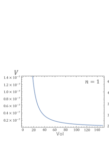
Figure 1: Modulus potential. The left one represents the modulus potential with $n=1,~{}\xi=10,~{}|f|=2.0\times 10^{-3},~{}|W_{0}|=1.0\times 10^{-2}$. The middle one represents the modulus potential with $n=2,~{}\xi=10,~{}|f|=2.0\times 10^{-2},~{}|W_{0}|=1.0\times 10^{-2}$. The right one represents the modulus potential with $n=3,~{}\xi=10,~{}|f|=2.0\times 10^{-4},~{}|W_{0}|=1.0\times 10^{-2}$.

When $n$ is equal to 3, the potential always has a nontrivial local minimum. If $\xi$ is negative, the minimum $\mathcal{V}_{0}$ is negative and it is not a valid stationary point, since the volume of the compact space must be positive. If $\xi$ is positive, the solutions are given by $\mathcal{V}_{0}=\frac{\xi}{4}\pm\frac{3|W_{0}|}{2f},$ and the potential is minimized by,

$$\mathcal{V}_{0}=\frac{\xi}{4}+\frac{3|W_{0}|}{2f}.$$ (2.19)

If either $|\frac{W_{0}}{f}|$ or $\xi$ is large enough, the Kähler modulus is stabilized at $\mathcal{V}_{0}\gg 1$. $\mathcal{V}_{0}\gg\xi$ for $|\frac{W_{0}}{f}|\gg\xi$.

When $n$ is larger than 3, the second term of (2.12) overcomes the prefactor $\frac{1}{(\mathcal{V}+\xi/4)^{2}}$, and it diverges to positive infinity as $\mathcal{V}\rightarrow\infty$. If $\xi$ is positive, (2.12) diverges to positive infinity as $\mathcal{V}\rightarrow\frac{\xi}{4}$, too, and we must have global minimum in the range of $\frac{\xi}{4}<\mathcal{V}$. If $\xi$ is negative and $|\frac{f}{W_{0}}|^{2}>(\frac{2}{|\xi|})^{2/3n}$, (2.12) diverges to positive infinity as $\mathcal{V}\rightarrow\frac{\xi}{4}$ and we have a nontrivial solution, too. Otherwise, we have no solutions.

In Figure 1, we show typical shapes of the potentials with $n=1,2,3$. It shows that large $n$ potentials stabilize the Kähler modulus.

On the other hand, when the $f$ in the superpotential is generated non-perturbatively, that is, $f$ is a function of $T$, the result of moduli stabilization is completely different. The superpotential is rewritten as

$$W=W_{0}-AXe^{-bT},$$ (2.20)

where the coefficient $A$ and $b$ are constant parameters. In this model the F-term potential is expanded as

$$V_{0}= \frac{1}{(\mathcal{V}+\frac{\xi}{4})^{2}}\left[\frac{3\xi}{4\mathcal{V}-\xi}|W_{0}|^{2}+A^{2}e^{-b(T+\bar{T})}\mathcal{V}^{2n/3}\right],$$ (2.21)

$$V_{1}= \frac{1}{(\mathcal{V}+\frac{\xi}{4})^{2}}\left[2\frac{2\mathcal{V}+\xi}{4\mathcal{V}-\xi}\left\{n-1-b(T+\bar{T})\right\}A\bar{W}_{0}e^{-bT}X+\mbox{h.c.}\right],$$ (2.22)

$$V_{2}= \tilde{m}_{X}^{2}|X|^{2}+\cdots.$$ (2.23)

When $\braket{X}$ is sufficiently small, we can approximate the modulus potential by the above $V_{0}$. $T$ is stabilized at the point satisfying the following equations,

$$V_{T}/|W_{0}|^{2} =\frac{3\mathcal{V}_{0}^{4/3}}{(\mathcal{V}_{0}+\frac{\xi}{2})^{3}}g(\mathcal{V}_{0})=0,$$ (2.24)

$$V_{TT}/|W_{0}|^{2} =\frac{9}{2}\frac{\mathcal{V}_{0}^{\frac{5}{3}}}{(\mathcal{V}_{0}+\frac{\xi}{2})^{3}}g^{\prime}(\mathcal{V}_{0})>0,$$ (2.25)

where $g(\mathcal{V})$ is given by

$$g(\mathcal{V})=-\frac{9}{8}\frac{\xi}{(\mathcal{V}-\frac{\xi}{4})^{2}}+\frac{f^{2}}{3|W_{0}|^{2}}e^{-b\mathcal{V}^{2/3}}\mathcal{V}^{2n/3-1}\left[\big{(}n-(3+b\mathcal{V}^{2/3})\big{)}+\frac{1}{2}\frac{\xi}{\mathcal{V}}(n-b\mathcal{V}^{2/3})\right].$$ (2.26)

When $\xi$ is positive, to realize $g(\mathcal{V})=0$, the first and the second terms of (2.26) must be balanced, which implies

$$\big{(}n-(3+b\mathcal{V}^{2/3})\big{)}+\frac{\xi}{2\mathcal{V}}(n-b\mathcal{V}^{2/3})>0.$$ (2.27)

Thus, we need $n>b\mathcal{V}^{2/3}.$ Here, $b\mathcal{V}^{2/3}$ is considered as an instanton action and it should be much larger than 1 for the single instanton approximation. $n$ is given by dimensional reduction, and it is typically of $\mathcal{O}(1)$ [15]. Therefore, we can not satisfy the stationary condition.

When $\xi$ is negative, there may be a stationary solution, but since there is the single Kähler modulus $T$ in our model, it is natural to assume that $(h_{1,2}-h_{1,1})>0$, hence $\xi$ is positive. Thus, this solution is invalid. We conclude that this form of superpotential can not stabilize the whole volume.

2.2 Consistency

Here, we examine the consistency of our model. Hereafter, we consider the case that the prefactor $f(T)$ is a constant.

For a consistent moduli stabilization, the compact space should be large enough to justify the supergravity approximation, i.e., $\mathcal{V}_{0}\gg 1$ in units of the string length. In our scenario, the size of the compact space is characterized by $\xi$ and $|\frac{W_{0}}{f}|^{2}$. For $n=2$, the stationary point is approximated by $\xi$. 3-dimensional Calabi-Yau manifolds admit variety of topologies and the Euler numbers [18]. It is possible to find a Calabi-Yau manifold whose Euler number is of $\mathcal{O}(10^{3})$, i.e. $\xi\sim 10$. Our moduli stabilization mechanism works well in such compactifications. For $n=3$, the stationary point is given by (2.19). The volume of the compact space is stabilized at a large volume when either of $|\frac{W_{0}}{f}|$ and $\xi$ is much larger than 1. We have a range of parameters to realize the consistency of the supergravity approximation.

Next, we also have to justify our assumptions that the mass of $X$ is much heavier than that of $T$ and the modulus potential terms proportional to $\braket{}{X}{}$ are negligible. The mass of $X$ is generated by quantum corrections [10, 17]. For a concrete discussion, we consider the O’Raifeartaigh-like model. To begin with, we briefly review the mass of $X$ generated by this model. Suppose that there are extra chiral superfields $\phi_{1}$ and $\phi_{2}$, and the superpotential is given by,

$$W=m\phi_{1}\phi_{2}+\lambda\phi_{1}^{2}X-fX.$$ (2.28)

For simplicity, we assume that Kähler metrics of these chiral superfields depend on heavy (stabilized) moduli other than $T$, and then we have canonically normalized their Kähler metrics; $K=|\phi_{1}|^{2}+|\phi_{2}|^{2}+|X|^{2}$. The masses $m$ of $\phi_{1,2}$ are relatively heavier than that of $X$, and we can integrate them out in order to study the dynamics of $X$. We consider the case of $\lambda f\ll m$, which means the VEVs of $\phi_{1}$ and $\phi_{2}$ are sufficiently small compared to the Planck mass. Integrating $\phi_{1}$ and $\phi_{2}$ out, we obtain the Coleman-Weinberg potential. It is interpreted as a correction to the Kähler potential and written as

$$W = -fX,$$

$$K = X\bar{X}\left(1-\frac{c\lambda^{2}}{16\pi^{2}}\log(1+\frac{\lambda^{2}X\bar{X}}{m^{2}})\right),$$ (2.29)

where we have assumed many $\phi_{1}$ and $\phi_{2}$, and the constant parameter $c$ denotes their multiplicity. Expanding the Kähler potential, we obtain

$$K\sim X\bar{X}-\frac{(X\bar{X})^{2}}{\Lambda^{2}},$$ (2.30)

where $\Lambda^{2}=\frac{16\pi^{2}m^{2}}{c\lambda^{4}}$. Then, the mass of $X$ comes from F-term potential; $e^{K}(K^{X\bar{X}}D_{X}WD_{\bar{X}}W-3|W|^{2})$. It is calculated as

$$V=f^{2}+\frac{4f^{2}}{\Lambda^{2}}X\bar{X}+\cdots,$$ (2.31)

and the mass of $X$ is $\frac{2f}{\Lambda}$. In our model, a similar mass term can be generated. The difference only comes from the Kähler potential. Since we postulate the Kähler potential is the sum of the Kähler potential of $T$ and that of $\phi_{i}$ and $X$, the mass of $X$ is given by

$$\tilde{m}_{X}^{2}=4e^{-2\log(\mathcal{V}+\xi/2)}\frac{f^{2}}{\Lambda^{2}}\sim 4\frac{f^{2}}{\Lambda^{2}}\mathcal{V}_{0}^{-2}.$$ (2.32)

To guarantee that $\phi_{1,2}$ are heavier than $X$, $\Lambda^{2}$ is much larger than $f$. The canonically normalized masses are calculated as

$$m_{X}^{2} =4\frac{f^{2}}{\Lambda^{2}}\mathcal{V}_{0}^{2n/3-2},$$ (2.33)

$$m_{T}^{2} =\frac{3}{2}\frac{\mathcal{V}_{0}^{\frac{4}{3}}}{(\mathcal{V}_{0}+\frac{\xi}{2})}\left[\left[\left(\frac{2}{3}n-2\right)\frac{1}{2\mathcal{V}_{0}}+\frac{1}{\mathcal{V}_{0}-\frac{\xi}{4}}\right]\frac{9}{4}\frac{\xi}{(\mathcal{V}_{0}-\frac{\xi}{4})^{2}}+\left(\frac{n}{3}-1\right)\left|\frac{f}{W_{0}}\right|^{2}\mathcal{V}_{0}^{\frac{2}{3}n-2}\right]|W_{0}|^{2}.$$ (2.34)

When $n$ is less than 3, $\mathcal{V}_{0}$ is characterized by $\xi$. We can estimate $m_{T}$ and $m_{X}$ as

$$m_{X}^{2} \sim 4\frac{f^{2}}{\Lambda^{2}}\left(\frac{\xi}{4}\right)^{2n/3-2},$$

$$m_{T}^{2} \sim \left(\frac{\xi}{4}\right)^{-\frac{5}{3}}\left[C_{1}+C_{2}\left|\frac{f}{W_{0}}\right|^{2}\left(\frac{\xi}{4}\right)^{\frac{2}{3}n}\right]|W_{0}|^{2},$$ (2.35)

where the parameters, $C_{1}$ and $C_{2}$, are of ${\mathcal{O}}(1)$. When $|\frac{f}{W_{0}}|$ is much less than 1, $m_{T}^{2}$ is approximated as $m_{T}^{2}\sim\left(\frac{\xi}{4}\right)^{-\frac{5}{3}}|W_{0}|^{2}$. The mass ratio is given as

$$\frac{m_{X}^{2}}{m_{T}^{2}}\sim\frac{1}{\Lambda^{2}}\frac{f^{2}}{|W_{0}|^{2}}\left(\frac{\xi}{4}\right)^{\frac{2n-1}{3}}.$$ (2.36)

$\frac{m_{X}^{2}}{m_{T}^{2}}\gg 1$ implies $\Lambda\ll 1$. On the other hand, when $|\frac{f}{W_{0}}|$ is much larger than 1, $m_{T}^{2}$ is approximated as $m_{T}^{2}\sim\left(\frac{\xi}{4}\right)^{\frac{2n}{3}-\frac{5}{3}}f^{2}$. The mass ratio is given as,

$$\frac{m_{X}^{2}}{m_{T}^{2}}\sim\frac{1}{\Lambda^{2}}\left(\frac{\xi}{4}\right)^{-\frac{1}{3}}.$$ (2.37)

It must be much greater than 1 since $\Lambda$ is measured in units of the Planck scale and $\Lambda<1$. In both cases, for $n<3$, a small $\Lambda$ justifies our assumption. When $n$ is equal to 3, $\mathcal{V}_{0}$ is given by (2.19). $m_{T}^{2}$ is given by

$$m_{T}^{2} =\frac{\mathcal{V}_{0}^{\frac{4}{3}}}{(\mathcal{V}_{0}+\frac{\xi}{2})}\frac{\xi f^{3}}{|W_{0}|}.$$ (2.38)

The ratio of the masses is written as

$$\frac{m_{X}^{2}}{m_{T}^{2}}=\frac{4}{\xi\Lambda^{2}}\frac{|W_{0}|}{f}\frac{\mathcal{V}_{0}^{4/3}}{\mathcal{V}_{0}+\frac{\xi}{2}}\sim\frac{4}{\xi\Lambda^{2}}\frac{|W_{0}|}{f}\mathcal{V}_{0}^{1/3}.$$ (2.39)

We can realize $m_{X}^{2}\gg m_{T}^{2}$ for $\frac{|W_{0}|^{2}}{f\xi\Lambda^{2}}\gg 1$.

Now, we examine our assumption that $\braket{X}\ll 1$. From (2.10) and (2.11), $\braket{}{X}{}$ is given by,

$$\braket{}{X}{}\sim\frac{(n-1)f|W_{0}|\mathcal{V}_{0}^{-2}}{\tilde{m}_{X}^{2}}.$$ (2.40)

Since $\tilde{m}_{X}$ is given by (2.32), $\braket{}{X}{}$ is calculated as

$$\braket{}{X}{}\sim\frac{(n-1)\Lambda^{2}|W_{0}|}{4f}.$$ (2.41)

To realize a small $\braket{}{X}{}$, we need $\Lambda^{2}\frac{|W_{0}|}{f}\ll 1$ in units of the Planck mass.

To illustrate the consistency conditions of our model, we study them for the case of $n=3$. In this case, the aforementioned conditions are written as follows,

$$3|W_{0}|\gg 2fM_{P},$$

$$6|W_{0}|^{2}\gg \xi f^{2}\Lambda^{2},$$

$$2fM_{P}^{3}\gg \Lambda^{2}|W_{0}|,$$

$$\Lambda^{4}\gg 4f^{2}.$$ (2.42)

We explicitly indicate the Planck mass which has been omitted. Roughly speaking, these conditions imply $|W_{0}|\gg fM_{P}$ and $\Lambda M_{P}\gg f$. There is a large range of parameters satisfying the above conditions. For example, $\xi=1,W_{0}=10^{-3},\Lambda=10^{-2},f=10^{-5},$ is a typical solution.

2.3 Cosmological Constant and Other Comments

In the above scenario, we can realize the modulus stabilization, where the potential minimum is given by (2.12), and the stationary point is given by (2.13). Then, we can approximate the vacuum energy as

$$V_{0}=|W_{0}|^{2}\frac{1}{(\mathcal{V}_{0}+\frac{\xi}{2})^{2}}\left(\frac{3\xi}{4(\mathcal{V}_{0}-\frac{\xi}{4})}+\frac{9\xi\mathcal{V}_{0}^{2}}{8(\mathcal{V}_{0}-\frac{\xi}{4})^{2}}\frac{1}{(\frac{n}{3}-1)\mathcal{V}_{0}+\frac{1}{6}n\xi}\right).$$ (2.43)

We can estimate

$$V_{0}\sim\frac{|W_{0}|^{2}}{M_{P}^{2}}\frac{1}{\ell_{s}^{18}\mathcal{V}_{0}^{-3}}.$$ (2.44)

This model has a positive cosmological constant. The vacuum energy is uplifted by the auxiliary component of $X$. It may be interesting that the vacuum energy is proportional to $\mathcal{V}_{0}^{-3}$. In order to realize the Minkowski vacuum, we need some effects to depress the vacuum energy.

We should also comment on the imaginary part of $T$, i.e. the axion. The axion is not stabilized in this scenario. That can be understood from the forms of the Kähler potential and the superpotential. We have shown that, in the superpotential (2.7), $f(T)$ must be a constant for the stabilization of $\tau$. The Kähler potential does not include the imaginary part of $T$ either. Thus the axion does not appear in the F-term potential. To stabilize it, we need to consider additional effects, for example, non-perturbative effects.

Although we have supposed the model that has one Kähler modulus only, we would apply this scenario to more general models that have many Kähler moduli. In general, the mass of Kähler moduli is suppressed by volume of the cycle related to the Kähler moduli, and the overall volume modulus would be lighter than the other Kähler moduli. In such cases, we can apply our moduli stabilization mechanism after the other moduli are stabilized by another stabilization mechanism, e.g. D-terms [21, 19], non-perturbative effects [3, 4, 5], etc.

Therefore, it is important to consider our moduli stabilization mechanism collaborated with another one, such as the KKLT scenario and the LVS. In the next section, we consider the latter one. We discuss the possibility of the F-term uplifting of the LVS by our model.

3 F-term Uplifting and the Large Volume Scenario

In this section, we study uplifting the AdS vacuum of the LVS to the Minkowski vacuum by adding one chiral superfield. First, we briefly review the LVS, and then, we study F-term uplifting mechanism.

3.1 Large Volume Scenario

The LVS was proposed in [4, 5] about 10 years ago. Here, we give a brief review on the LVS. In this scenario, the Kähler moduli are stabilized at the point where the $\alpha^{\prime}$ corrections and the non-perturbative effects are balanced. In this paper, we study the LVS based on swiss cheese compactifications, which means that the dimensionless volume of the Calabi-Yau space is given like

$$\mathcal{V}=(T_{1}+\bar{T}_{1})^{3/2}-\sum_{i>1}\gamma_{i}(T_{i}+\bar{T}_{i})^{3/2},$$ (3.1)

where $T_{i}$ represents a volume modulus corresponding to the $i$-th 4-cycle on the Calabi-Yau manifold, and $\gamma_{i}$ is a geometrical parameter. With perturbative $\alpha^{\prime}$ corrections and non-perturbative effects taken into account, the Kähler potential and the superpotential can be represented as follows,

$$K=-2\log\left[\mathcal{V}+\frac{\xi}{2}\right],\qquad W=W_{0}+\sum_{i>1}A_{i}e^{-a_{i}T_{i}}.$$ (3.2)

Calculating (2.1), the scalar potential is given as

$$V_{LVS}= \frac{A}{\mathcal{V}^{3}}-\sum_{i>1}\frac{B_{i}a_{i}\tau_{i}e^{-a_{i}\tau_{i}}}{\mathcal{V}^{2}}+\sum_{i>1}\frac{C_{i}\sqrt{a_{i}\tau_{i}}e^{-2a_{i}\tau_{i}}}{\mathcal{V}}+\mathcal{O}(\mathcal{V}^{-4}),$$ (3.3)

where $A,B_{i},C_{i}$ are given as,

$$A=\frac{3\xi|W_{0}|^{2}}{4},~{}~{}B_{i}=4A_{i}|W_{0}|,~{}~{}C_{i}=\frac{2\sqrt{2}a_{i}^{3/2}A_{i}^{2}}{3\gamma_{2}}.$$ (3.4)

The minimum of the potential is given by the point satisfying the following equations,

$$A=\sum_{i>1}\frac{B_{i}^{2}(a_{i}\tau_{i})^{3/2}}{4C_{i}}\frac{a_{i}\tau_{i}(a_{i}\tau_{i}-1)}{(a_{i}\tau_{i}-1/4)^{2}},\qquad\mathcal{V}=\frac{1}{2}\frac{B_{i}}{C_{i}}\sqrt{a_{i}\tau_{i}}e^{a_{i}\tau_{i}}\frac{a_{i}\tau_{i}-1}{a_{i}\tau_{i}-1/4}.$$ (3.5)

When $a_{i}\tau_{i}$ is much larger than 1, the solution is approximated by,

$$\tau_{i}\sim\frac{1}{a_{i}}\left(\frac{4A}{\sum_{i>1}\frac{B_{i}^{2}}{C_{i}}}\right)^{2/3},\qquad\mathcal{V}\sim\frac{1}{2}\frac{B_{i}}{C_{i}}\sqrt{a_{i}\tau_{i}}e^{a_{i}\tau_{i}}.$$ (3.6)

As the results, all the Kähler moduli are stabilized successfully. The volume of the compact space is stabilized at an exponentially large value compared to $\tau_{i}$.

The vacuum of the LVS breaks SUSY. In fact, the auxiliary fields of the Kähler moduli are not zero. However, its vacuum is still an AdS vacuum. The minimum value of the potential is calculated as,

$$V_{minimum}\sim-\frac{A}{2a_{i}\braket{\tau_{i}}\braket{\mathcal{V}}^{3}}+\mathcal{O}(\mathcal{V}^{-4}),$$ (3.7)

and it is negative.

In the original paper, anti D-branes are introduced for uplifting. Here, we study uplifting by the chiral superfield $X$.

3.2 F-term Uplifting

We study moduli stabilization and uplifting simultaneously. Suppose that there are two Kähler moduli, $T_{1},T_{2}$ and one chiral superfield $X$. Their Kähler potential and the volume of the compact space are given by,

$$K=-2\log\left[\mathcal{V}+\frac{\xi}{2}\right]+(T_{2}+\bar{T}_{2})^{-m}(T_{1}+\bar{T}_{1})^{-n}|X|^{2},$$ (3.8)

$$\mathcal{V}=(T_{1}+\bar{T}_{1})^{3/2}-\gamma_{2}(T_{2}+\bar{T}_{2})^{3/2}.$$ (3.9)

Similar to the previous section, we consider two forms of superpotential,

$$W= W_{0}-fX+A_{2}e^{-a_{2}T_{2}},$$ (3.10)

and

$$W= W_{0}-A\,e^{-bT_{2}}X,$$ (3.11)

where $f,\,a_{2},\,A_{2},\,A$ and $b$ are real constants. The superpotential (3.10) and (3.11) correspond to the case that the $f(T)X$ term are induced by perturbative and non-perturbative effects respectively. We assume that $W_{0}$ is real for simplicity. In both cases, we expect that the mass of $X$ is generated by radiative corrections and the scalar potential is given by,

$$V=e^{K}\left[K^{i\bar{j}}D_{i}WD_{\bar{j}}\bar{W}-3|W|^{2}\right]+\tilde{m}_{X}^{2}|X|^{2}.$$ (3.12)

We also assume that $X$ is much heavier than the other moduli, and we can integrate $X$ out before studying the Kähler moduli stabilization. We confirm the validity of this assumption later.

We expand $V$ in terms of $X$ as,

$$V(T_{1},T_{2},X)=V_{0}(T_{1},T_{2})+V_{1}(T_{1},T_{2},X)+V_{2}(T_{1},T_{2},X)+\cdots,$$ (3.13)

where $V_{i}$ is the $i$-th order term of $X$. For the case of (3.10), we obtain

$$V_{0} =V_{LVS}(T_{1},T_{2})+\frac{1}{(\mathcal{V}+\frac{\xi}{2})^{2}}(T_{1}+\bar{T}_{1})^{n}(T_{2}+\bar{T}_{2})^{m}f^{2},$$ (3.14)

$$V_{1} =\frac{1}{\mathcal{V}^{2}}\left[-(1+m)f\left(W_{0}+A_{2}e^{-a_{2}\bar{T}_{2}}\right)\bar{X}+m(2\tau_{2})^{-1/2}\frac{2\mathcal{V}}{3\gamma_{2}}f\left(-A_{2}a_{2}e^{-a_{2}\bar{T}_{2}}\right)\bar{X}+h.c.\,\right]+\cdots,$$ (3.15)

$$V_{2} =\tilde{m}_{X}^{2}|X|^{2}+\cdots,$$ (3.16)

where $V_{LVS}$ is the moduli potential of the LVS and the ellipses represent the higher order terms of $\mathcal{V}^{-1}$. Using (3.6), we can approximate $V_{1}$ as,

$$V_{1} \sim\frac{1}{\mathcal{V}^{2}}\left[(-1+(3\sqrt{2}-1)m)fW_{0}\bar{X}+h.c.\,\right]+\cdots.$$ (3.17)

Then, the approximated VEV of $X$ is given by

$$\braket{X}\sim\frac{f}{\mathcal{V}^{2}}\frac{(-1+(3\sqrt{2}-1)m)W_{0}}{\tilde{m}_{X}^{2}}.$$ (3.18)

Since $V_{LVS}$ is of $\mathcal{O}(\mathcal{V}^{-3})$, $\mathcal{O}(\braket{X}^{2})$ term is negligible. After integrating $X$ out, the moduli potential $\tilde{V}$ is evaluated as

$$\tilde{V}= V_{LVS}(\tau_{1},\tau_{2})+f^{\prime 2}\mathcal{V}^{-2}(\tau_{1})^{n}(\tau_{2})^{m}+\mathcal{O}(\mathcal{V}^{-4}),$$

$$\sim V_{LVS}(\tau_{1},\tau_{2})+f^{\prime 2}\mathcal{V}^{\frac{2}{3}n-2}(\tau_{2})^{m},$$ (3.19)

$$V_{LVS}= \frac{A}{\mathcal{V}^{3}}-\frac{Ba_{2}\tau_{2}e^{-a_{2}\tau_{2}}}{\mathcal{V}^{2}}+\frac{C\sqrt{a_{2}\tau_{2}}e^{-2a_{2}\tau_{2}}}{\mathcal{V}}+\mathcal{O}(\mathcal{V}^{-4}),$$ (3.20)

$$A= \frac{3\xi|W_{0}|^{2}}{4},~{}~{}B=4A_{2}|W_{0}|,~{}~{}C=\frac{2\sqrt{2}a_{2}^{3/2}A_{2}^{2}}{3\gamma_{2}},~{}~{}f^{\prime 2}=2^{n+m}f^{2}.$$ (3.21)

We see that the potential is uplifted by $f^{\prime 2}\mathcal{V}^{2n/3-2}(\tau_{2})^{m}$. If $f^{\prime}$ is sufficiently small such that the stationary point of our model is approximated by that of the LVS, its vacuum energy is approximated as

$$\tilde{V}(\mathcal{V}_{0},\tau_{2,0})=-\frac{A_{2}}{a_{2}\tau_{2,0}\mathcal{V}_{0}^{3}}+|f^{\prime}|^{2}\mathcal{V}_{0}^{2n/3-2}(\tau_{2,0})^{m},$$ (3.22)

where ($\mathcal{V}_{0}$,$\tau_{2,0}$) is the minimum point of the LVS potential. The Minkowski vacuum can be realized by,

$$|f^{\prime}|^{2}=\frac{A}{2a_{2}}\mathcal{V}_{0}^{-2n/3-1}(\tau_{2,0})^{-m-1}.$$ (3.23)

More precisely, the stationary point of our model is perturbed from that of the LVS. The true minimum is represented by,

$$\mathcal{V}=\mathcal{V}_{0}+\delta_{\mathcal{V}},$$ (3.24)

$$\tau_{2}=\tau_{2,0}+\delta_{\tau}.$$ (3.25)

We assume $\delta_{\mathcal{V}}/\mathcal{V}_{0},\delta_{\tau}/\tau_{2,0}\ll 1$. Using (3.23), we can calculate the leading order deviations from the vacuum of the LVS as follows,

$$\frac{\partial\tilde{V}}{\partial\tau_{2}}= \frac{a_{2}}{\mathcal{V}^{2}}\left[B(a_{2}\tau_{2}-1)e^{-a_{2}\tau_{2}}-C\mathcal{V}\left(2a_{2}\tau_{2}-\frac{1}{2}\right)\frac{e^{-2a_{2}\tau_{2}}}{\sqrt{a_{2}\tau_{2}}}\right]+\frac{A}{2a_{2}}m\frac{\mathcal{V}^{2n/3-2}}{\mathcal{V}_{0}^{2n/3+1}}\frac{(\tau_{2})^{m-1}}{(\tau_{2,0})^{m+1}}=0,$$ (3.26)

$$\frac{\partial\tilde{V}}{\partial\mathcal{V}}= -\frac{3A}{\mathcal{V}^{4}}+\frac{2Ba_{2}\tau_{2}e^{-a_{2}\tau_{2}}}{\mathcal{V}^{3}}-\frac{C\sqrt{a_{2}\tau_{2}}e^{-2a_{2}\tau_{2}}}{\mathcal{V}^{2}}+\frac{A}{2a_{2}}(\frac{2n}{3}-2)\frac{\mathcal{V}^{2n/3-3}}{\mathcal{V}_{0}^{2n/3+1}}\frac{(\tau_{2})^{m}}{(\tau_{2,0})^{m+1}}=0.$$ (3.27)

That is, the deviations of the VEVs are estimated as,

$$\frac{\delta_{\tau}}{\tau_{2,0}}=\frac{1}{x_{0}}\frac{2(\frac{n}{3}-1)}{5+2(\frac{n}{3}-1)(\frac{2n}{3}-3)}+\mathcal{O}(x_{0}^{-2}),$$ (3.28)

$$\frac{\delta_{\mathcal{V}}}{\mathcal{V}_{0}}=\frac{2}{5+2(\frac{n}{3}-1)(\frac{2n}{3}-3)}\frac{m}{2}+\mathcal{O}(x_{0}^{-1}),$$ (3.29)

where $x_{0}=a_{2}\tau_{2,0}$. The vacuum of the LVS implies that $a_{2}\tau_{2,0}$ is of $\mathcal{O}(10)$. Thus, $\delta_{\tau}/\tau_{2,0}$ is suppressed. On the other hand, there is no suppression factor for the deviation of the whole volume $\delta_{\mathcal{V}}/\mathcal{V}_{0}$, and it seems to be of $\mathcal{O}(1)$. However, since the denominator of (3.29) is of $\mathcal{O}(10)$, $\delta_{\mathcal{V}}/\mathcal{V}_{0}$ is successfully suppressed and of $\mathcal{O}(10^{-1})$. Therefore, the deviations are indeed small. The typical values of $\delta_{\mathcal{V}}/\mathcal{V}_{0}$ are summarized in Table 1, and we can confirm that the range of $\delta_{\mathcal{V}}/\mathcal{V}_{0}$ is small. The uplifting term does not destabilize the vacuum of the LVS drastically. Our rough estimation is valid and we can successfully uplift the vacuum energy of the LVS.

$m\backslash n$	0	1	2	3
0	0	0	0	0
1	1/22	9/146	9/110	1/10
2	1/11	9/73	9/55	1/5
3	3/22	27/146	27/110	3/10

Table 1: Typical values of $|\delta_{\mathcal{V}}/\mathcal{V}_{0}|$. The column represents $m$ and the row is $n$.

Finally, we study the mass of $X$. The heaviest mode of the Kähler moduli is the small volume moduli $\tau_{2}$, and its canonically normalized mass $m_{\tau_{2}}$ is estimated in [5] as

$$m_{\tau_{2}}^{2}\sim\left(\frac{W_{0}}{\sqrt{4\pi}\mathcal{V}_{0}}\right)^{2}.$$ (3.30)

The mass squared of $X$ is given by (2.33). Substituting $f$ by (3.23), the mass of $X$ is estimated as

$$m_{X}^{2}\sim 4\frac{f^{2}}{\Lambda^{2}}\mathcal{V}_{0}^{\frac{2}{3}n-2}\sim 3\xi(\tau_{2,0})^{-m-1}\frac{W_{0}^{2}}{2a_{2}\Lambda^{2}}\mathcal{V}_{0}^{-3}.$$ (3.31)

Roughly speaking, $X$ is heavier than $T$ for $\Lambda^{-2}>\mathcal{V}_{0}$. For instance, when $\mathcal{V}_{0}\sim 10^{6}$, $\Lambda$ should be smaller than $10^{-3}M_{P}$. When the above condition is satisfied, we can safely integrate $X$ out before the Kähler moduli stabilization, and succeed to uplift the vacuum energy.

On the other hand, if the superpotential of $X$ includes the dependence of Kähler moduli $T_{i}$, that is, the superpotential is given as (3.11), the result is completely different. Expanding its scalar potential in term of $X$ and integrating $X$ out, we obtain moduli potential,

$$V_{0} =\frac{1}{(\mathcal{V}+\frac{\xi}{2})^{2}}\left[-\frac{3}{4}\frac{\xi}{\mathcal{V}-\frac{\xi}{4}}|W_{0}|^{2}+(T_{1}+\bar{T}_{1})^{n}(T_{2}+\bar{T}_{2})^{m}A^{2}e^{-2b\tau_{2}}\right].$$ (3.32)

Its stationary point must satisfy the following conditions,

$$\frac{\partial V}{\partial\tau_{2}}\sim \frac{2(2\tau_{1})^{n}(2\tau_{2})^{m-1}A^{2}e^{-2b\tau_{2}}}{(\mathcal{V}+\frac{\xi}{2})^{2}}\left[m-2b\tau_{2}\right]=0,$$ (3.33)

$$\frac{\partial^{2}V}{\partial\tau_{2}^{2}}\sim \left(\frac{\partial}{\partial\tau_{2}}\frac{2(2\tau_{1})^{n}(2\tau_{2})^{m-1}A^{2}e^{-2b\tau_{2}}}{(\mathcal{V}+\frac{\xi}{2})^{2}}\right)\left[m-2b\tau_{2}\right]-\frac{4b(2\tau_{1})^{n}(2\tau_{2})^{m-1}A^{2}e^{-2b\tau_{2}}}{(\mathcal{V}+\frac{\xi}{2})^{2}}>0,$$ (3.34)

where we used that $\tau_{1}$ is much larger than 1. Since $\partial V/\partial\tau_{2}=0$ implies $m=2b\tau_{2}$, there are no stable vacua. Such a superpotential destabilizes the LVS vacuum. Hereafter, we treat $f(T)$ as a constant parameter and the superpotential is written as (3.10).

3.3 Numerical Analysis

In the previous subsection, we considered the LVS model uplifted by the chiral superfield. We confirmed that if $f(T)$ is a constant the vacuum of the LVS can be uplifted to the Minkowski vacuum successfully, by expanding the moduli potential in terms of the deviations from the vacuum of the LVS. Here, we examine the previous conclusion numerically. In Fig.2, we show the shape of a potential of the LVS (left) and that of the uplifted LVS (right). In Fig.2, we set $A=1,B=0.2,C=1,a_{2}=2\pi$. In this case, the approximated minimum of the original LVS (3.6) is calculated as,

$$\mathcal{V}_{0}=1.055\times 10^{9},~{}\tau_{2,0}=3.429,$$ (3.35)

and the numerical result is

$$\mathcal{V}_{0}^{Num}=1.449\times 10^{9},~{}\tau_{2,0}^{Num}=3.484.$$ (3.36)

The value of the potential minimum is well approximated. From (3.23), we get the value of $f^{\prime}$ that uplifts the minimum to the Minkowski vacuum. When $n=1,~{}m=2$, the value of $f^{\prime}$ is calculated using the approximated solution and numerical solution;

$$f^{\prime 2}\sim 1.344\times 10^{-9},~{}~{}~{}f_{Num}^{\prime 2}\sim 1.007\times 10^{-9}.$$ (3.37)

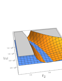
Figure 2: Moduli potential of the LVS (left) and that of the uplifted LVS (right). We set $A=1,~{}B=0.2,~{}C=1,~{}a_{2}=2\pi,~{}n=1,~{}m=2,~{}f^{\prime 2}=1.00742\times 10^{-9}$. Here, in order to visualize the minimum easily, we use the value of f’ in the numerical solution. The orange surfaces denote the moduli potentials and the blue surface is the $V=0$. You can see that the vacuum energy of the LVS is negative, but that of the uplifted LVS is almost zero.

Analytical calculation of the potential minimum of the uplifted LVS is difficult. We only illustrate the existence of the minimum of the uplifted LVS and its rough position by Fig.2. The orange surface represents the potential of the LVS and the uplifted LVS. The blue surface is $V=0$. In the left figure, there is a large region where the moduli potential is negative around the curve of $\mathcal{V}\sim\frac{1}{2}\frac{B_{i}}{C_{i}}\sqrt{a_{i}\tau_{i}}e^{a_{i}\tau_{i}}$. Thus its potential minimum is definitely negative. However, in the right figure, the orange surface is above the blue surface in almost all of the region. The potential minimum must be located in a small region at the upper-left corner of the right figure, where the blue surface overcomes the orange surface. This small region includes $(\mathcal{V}_{0},\tau_{2,0})$. The deviations from the vacuum of the LVS is not so drastic. The potential is almost uplifted by $X$. We conclude that our uplifting mechanism works well.

3.4 F-terms

In this subsection, we study the auxiliary components of the Kähler moduli fields and $X$. F-term SUSY breaking is characterized by the VEV of the auxiliary components of chiral superfields. They are given by,

$$F^{\bar{i}}=-e^{-K/2}K^{\bar{i}j}D_{j}W.$$ (3.38)

$D_{T_{1}}W,D_{T_{2}}W,D_{X}W$ are estimated by,

$$D_{T_{1}}W =\left[\frac{-3(2\tau_{1})^{1/2}}{\mathcal{V}+\frac{\xi}{2}}(W_{0}+e^{-a_{2}\tau_{2}})\right]\sim\mathcal{V}_{0}^{-2/3},$$ (3.39)

$$D_{T_{2}}W =\left[A_{2}a_{2}e^{-a_{2}T_{2}}+\frac{3\gamma_{2}(2\tau_{2})^{1/2}}{\mathcal{V}+\frac{\xi}{2}}(W_{0}+e^{-a_{2}\tau_{2}})\right]\sim\mathcal{V}_{0}^{-1},$$ (3.40)

$$D_{X}W =\left[-f+(2\tau_{1})^{-n}(2\tau_{2})^{-m}\braket{X}(W_{0}+e^{-a_{2}\tau_{2}})\right]\sim\mathcal{V}_{0}^{-n/3-1/2}.$$ (3.41)

We used that $\braket{X}$ is of $\mathcal{O}(\mathcal{V}_{0}^{-2})$ and its linear term is a subleading term. $K_{i\bar{j}}$ and $K^{i\bar{j}}$ are calculated as,

$$K_{i\bar{j}} \sim\begin{pmatrix}\mathcal{V}_{0}^{-2n/3}&0&0\\ 0&\mathcal{V}_{0}^{-4/3}&\mathcal{V}_{0}^{-5/3}\\ 0&\mathcal{V}_{0}^{-5/3}&\mathcal{V}_{0}^{-1}\end{pmatrix},$$ (3.42)

$$K^{i\bar{j}} \sim\begin{pmatrix}\mathcal{V}_{0}^{2n/3}&0&0\\ 0&\mathcal{V}_{0}^{4/3}&\mathcal{V}_{0}^{2/3}\\ 0&\mathcal{V}_{0}^{2/3}&\mathcal{V}_{0}\end{pmatrix}.$$ (3.43)

The VEVs of the F-terms are estimated as,

$$F^{X} =-\frac{1}{\mathcal{V}+a}K^{X\bar{X}}D_{X}W\sim\mathcal{V}_{0}^{\frac{n}{3}-\frac{3}{2}},$$ (3.44)

$$F^{T_{1}} =-\frac{1}{\mathcal{V}+a}(K^{T_{1}\bar{T}_{1}}D_{T_{1}}W+K^{T_{1}\bar{T}_{2}}D_{T_{2}}W)\sim\mathcal{V}_{0}^{-1/3},$$ (3.45)

$$F^{T_{2}} =-\frac{1}{\mathcal{V}+a}(K^{T_{2}\bar{T}_{1}}D_{T_{1}}W+K^{T_{2}\bar{T}_{2}}D_{T_{2}}W)\sim\mathcal{V}_{0}^{-1}.$$ (3.46)

Thus, if $n$ is larger than $\frac{7}{2}$, we obtain $\mathcal{V}_{0}^{\frac{n}{3}-\frac{3}{2}}\sim F^{X}\gg F^{T_{1}}\gg F^{T_{2}}\sim\mathcal{V}_{0}^{-1}$. If $\frac{7}{2}>n>\frac{3}{2}$, we find $\mathcal{V}_{0}^{-1/3}\sim F^{T_{1}}\gg F^{X}\gg F^{T_{2}}\sim\mathcal{V}_{0}^{-1}$, and if $n$ is smaller than $\frac{3}{2}$, we have $\mathcal{V}_{0}^{-1/3}\sim F^{T_{1}}\gg F^{T_{2}}\gg F^{X}\sim\mathcal{V}_{0}^{\frac{n}{3}-\frac{3}{2}}$.

On the other hand, the gravitino mass $m_{3/2}$ is independent of $n$, and it is given by,

$$m_{3/2}=e^{K/2}W_{0}\sim\mathcal{V}_{0}^{-1}.$$ (3.47)

Using the above equations, we can calculate soft terms. Although $F^{X}$ can overcome or be comparable to $F^{T_{1},T_{2}}$, the soft masses are not affected from those of the LVS.

4 Conclusion and Discussion

We have studied the new type of Kähler moduli stabilization and the F-term uplifting of the Large Volume Scenario. For realistic string models, moduli stabilization is crucial. In addition, since our universe has a positive cosmological constant, there must be a source of uplifting in superstring theory.

First, we have investigated whether the chiral superfield $X$ which is coupled with the whole volume in the Kähler potential can stabilize the Kähler modulus or not. The mass of $X$ is much heavier than the Kähler modulus and the VEV $\langle X\rangle$ is almost negligible, but its F-term potential can affect the moduli potential. We assumed that the superpotential is written as $W=W_{0}-f(T)X$ and Kähler potential is given as $K=-2\ln(\mathcal{V}+\frac{\xi}{2})+(T+\bar{T})^{-n}|X|^{2}$. We showed that if $f$ is a constant and $n$ is equal to 3 or larger, the whole volume of the extra dimension can be successfully stabilized. When $n=2$, the modulus potential has a nontrivial stationary point, but its value is too small for the leading order approximation in terms of $\alpha^{\prime}$ of the Kähler potential. If the higher order corrections remains subdominant, our moduli stabilization mechanism works well even for $n=2$. If $f$ is generated non-perturbatively, i.e. $f=f(T)$, the modulus potential has no stationary points and the Kähler modulus can not be stabilized. Thus, the form of the superpotential is very important for the modulus stabilization. We also studied the condition for heavy $X$. The mass scale of $X$ must be heavier than that of Kähler modulus. We explicitly show the parameter set satisfying the consistency conditions for $n=3$.

However, our moduli stabilization scenario has a few drawbacks. To stabilize the axions and other Kähler moduli, extra moduli stabilization mechanisms are required. The energy density of the stationary point is positive definite, and it must be depressed by another mechanism. Hence, it is important to consider this moduli stabilization mechanism collaborated with another one. In this paper, we consider it with the Large Volume Scenario. In this case, the chiral superfield $X$ plays as a source of the F-term uplifting.

In the original LVS, the vacuum energy is uplifted by anti D-branes. In this paper, we studied F-term uplifting of the LVS vacuum by the chiral superfield. We found that F-term uplifting requires a certain form of the superpotential too. We need the $T_{i}$ independent $fX$ term in the superpotential. If such a superpotential is induced, the vacuum energy of the LVS can be uplifted to the Minkowski vacuum (or de Sitter vacuum) by fine tuning the prefactor $f$.

In both cases, the form of the superpotentials is crucial. The superpotential including $X$ is written as

$$W=W_{0}-f(T)X.$$ (4.1)

$f$ must be a constant for the moduli stabilization and the F-term uplifting, otherwise it destabilizes the moduli stabilization mechanism completely. For example, such a constant prefactor may be induced by non-perturbative effects on D3-brane (or D(-1)-brane instanton). Since it is suppressed by $e^{-S}$, where $S$ is the dilaton. $S$ is stabilized by a 3-form flux at the tree level, and it can be substituted by its VEV. Another possibility is non-perturbative effects on D7-branes (D3-brane instantons) wrapping 4-cycles whose sizes are already stabilized by other effects. Such a mechanism may be provided by D-terms in magnetized D-branes or other flux effects. Studying a concrete origin of such a superpotential in superstring theory would be interesting.

References

- [1] L. E. Ibanez and A. M. Uranga, “String theory and particle physics: An introduction to string phenomenology,” Cambridge University Press (2012).
- [2] R. Blumenhagen, B. Kors, D. Lust and S. Stieberger, Phys. Rept. 445, 1 (2007) [hep-th/0610327].
- [3] S. Kachru, R. Kallosh, A. D. Linde and S. P. Trivedi, Phys. Rev. D 68, 046005 (2003) doi:10.1103/PhysRevD.68.046005 [hep-th/0301240].
- [4] V. Balasubramanian, P. Berglund, J. P. Conlon and F. Quevedo, JHEP 0503, 007 (2005) doi:10.1088/1126-6708/2005/03/007 [hep-th/0502058].
- [5] J. P. Conlon, F. Quevedo and K. Suruliz, JHEP 0508, 007 (2005) doi:10.1088/1126-6708/2005/08/007 [hep-th/0505076].
- [6] S. Gukov, C. Vafa and E. Witten, Nucl. Phys. B 584, 69 (2000) Erratum: [Nucl. Phys. B 608, 477 (2001)] [hep-th/9906070].
- [7] H. Abe, T. Higaki and T. Kobayashi, Phys. Rev. D 76, 105003 (2007) doi:10.1103/PhysRevD.76.105003 [arXiv:0707.2671 [hep-th]].
- [8] H. Abe, T. Higaki, T. Kobayashi and Y. Omura, Phys. Rev. D 75, 025019 (2007) doi:10.1103/PhysRevD.75.025019 [hep-th/0611024].
- [9] E. Dudas, C. Papineau and S. Pokorski, JHEP 0702, 028 (2007) doi:10.1088/1126-6708/2007/02/028 [hep-th/0610297].
- [10] R. Kallosh and A. D. Linde, JHEP 0702, 002 (2007) doi:10.1088/1126-6708/2007/02/002 [hep-th/0611183].
- [11] A. Achucarro and K. Sousa, JHEP 0803, 002 (2008) doi:10.1088/1126-6708/2008/03/002 [arXiv:0712.3460 [hep-th]].
- [12] P. Candelas and X. de la Ossa, Nucl. Phys. B 355, 455 (1991). doi:10.1016/0550-3213(91)90122-E
- [13] T. Kobayashi, N. Omoto, H. Otsuka and T. H. Tatsuishi, Phys. Rev. D 96, no. 4, 046004 (2017) [arXiv:1704.04875 [hep-th]]; Phys. Rev. D 97, no. 10, 106006 (2018) doi:10.1103/PhysRevD.97.106006 [arXiv:1711.10274 [hep-th]].
- [14] K. Becker, M. Becker, M. Haack and J. Louis, JHEP 0206, 060 (2002) doi:10.1088/1126-6708/2002/06/060 [hep-th/0204254].
- [15] M. Grana, T. W. Grimm, H. Jockers and J. Louis, Nucl. Phys. B 690, 21 (2004) [hep-th/0312232]; J. P. Conlon, D. Cremades and F. Quevedo, JHEP 0701, 022 (2007) [hep-th/0609180]; H. Jockers and J. Louis, Nucl. Phys. B 705, 167 (2005) [hep-th/0409098].
- [16] H. Abe, T. Kobayashi and K. Sumita, Nucl. Phys. B 911, 606 (2016) doi:10.1016/j.nuclphysb.2016.08.030 [arXiv:1605.02922 [hep-th]].
- [17] L. O’Raifeartaigh, Nucl. Phys. B 96, 331 (1975). doi:10.1016/0550-3213(75)90585-4
- [18] M. Kreuzer and H. Skarke, Adv. Theor. Math. Phys. 4, 1209 (2002) [hep-th/0002240]. S. B. Johnson and W. Taylor, JHEP 1410, 23 (2014) [arXiv:1406.0514 [hep-th]].
- [19] P. Fayet and J. Iliopoulos, Phys. Lett. 51B, 461 (1974); C. P. Burgess, R. Kallosh and F. Quevedo, JHEP 0310, 056 (2003) [hep-th/0309187]; R. Blumenhagen, D. Lust and T. R. Taylor, Nucl. Phys. B 663, 319 (2003) [hep-th/0303016].
- [20] S. Krippendorf and F. Quevedo, JHEP 0911, 039 (2009) doi:10.1088/1126-6708/2009/11/039 [arXiv:0901.0683 [hep-th]].
- [21] H. Abe, T. Kobayashi, K. Sumita and S. Uemura, Phys. Rev. D 96, no. 2, 026019 (2017) [arXiv:1703.03402 [hep-th]].