Counterfactual Critic Multi-Agent Training for Scene Graph Generation

Abstract

Scene graphs — objects as nodes and visual relationships as edges — describe the whereabouts and interactions of objects in an image for comprehensive scene understanding. To generate coherent scene graphs, almost all existing methods exploit the fruitful visual context by modeling message passing among objects. For example, “person” on “bike” can help to determine the relationship “ride”, which in turn contributes to the confidence of the two objects. However, we argue that the visual context is not properly learned by using the prevailing cross-entropy based supervised learning paradigm, which is not sensitive to graph inconsistency: errors at the hub or non-hub nodes should not be penalized equally. To this end, we propose a Counterfactual critic Multi-Agent Training (CMAT) approach. CMAT is a multi-agent policy gradient method that frames objects into cooperative agents, and then directly maximizes a graph-level metric as the reward. In particular, to assign the reward properly to each agent, CMAT uses a counterfactual baseline that disentangles the agent-specific reward by fixing the predictions of other agents. Extensive validations on the challenging Visual Genome benchmark show that CMAT achieves a state-of-the-art performance by significant gains under various settings and metrics.

1 Introduction

Figure 1: (a) An input image and its ground-truth scene graph. (b) For graph-coherent objective, a graph-level metric will penalize the red node more than $(>)$ the blue one, even though both are misclassified as man. (c) For local-sensitive objective, the individual reward for predicting the red node as bike can be identified by excluding $(-)$ the reward from non-bike predictions.

Visual scene understanding, e.g., what and where the things and stuff are, and how they relate with each other, is one of the core tasks in computer vision. With the maturity of object detection [49, 34] and segmentation [35, 16], computers can recognize object categories, locations, and visual attributes well. However, scene understanding goes beyond the whereabouts of objects. A more crucial step is to infer their visual relationships — together with the objects, they offer comprehensive and coherent visually-grounded knowledge, called scene graphs [23]. As shown in Figure 1 (a), the nodes and edges in scene graphs are objects and visual relationships, respectively. Moreover, scene graph is an indispensable knowledge representation for many high-level vision tasks such as image captioning [69, 66, 68, 24], visual reasoning [53, 14], and VQA [42, 19].

A straightforward solution for Scene Graph Generation (SGG) is in an independent fashion: detecting object bounding boxes by an existing object detector, and then predicting the object classes and their pairwise relationships separately [37, 74, 67, 52]. However, these methods overlook the fruitful visual context, which offers a powerful inductive bias [9] that helps object and relationship detection. For example in Figure 1, window and building usually co-occur within an image, and near is the most common relationship between tree and building; it is easy to infer that ? is building from window-on-? or tree-near-?. Such intuition has been empirically shown benefits in boosting SGG [62, 7, 28, 30, 29, 71, 20, 73, 58, 13, 44, 59, 45]. More specifically, these methods use a conditional random field [79] to model the joint distribution of nodes and edges, where the context is incorporated by message passing among the nodes through edges via a multi-step mean-field approximation [26]; then, the model is optimized by the sum of cross-entropy (XE) losses of nodes (e.g., objects) and edges (e.g., relationships).

Nevertheless, the coherency of the visual context is not captured effectively by existing SGG methods due to the main reason: the XE based training objective is not graph-coherent. By “graph-coherent”, we mean that the quality of the scene graph should be at the graph-level: the detected objects and relationships should be contextually consistent; however, the sum of XE losses of objects and relationships is essentially independent. To see the negative impact of this inconsistency, suppose that the red and the blue nodes are both misclassified in Figure 1 (b). Based on the XE loss, the errors are penalized equally. However, the error of misclassifying the red node should be more severe than the blue one, as the red error will influence more nodes and edges than the blue one. Therefore, we need to use a graph-level metric such as Recall@K [37] and SPICE [1] to match the graph-coherent objective, which penalizes more for misclassifying important hub nodes than others. Meanwhile, the training objective of SGG should be local-sensitive. By “local-sensitive”, we mean that the training objective is sensitive to the change of a single node. However, since the graph-coherent objective is a global pooling quantity, the individual contribution of the prediction of a node is lost. Thus, we need to design a disentangle mechanism to identify the individual contribution and provide an effective training signal for each local prediction.

In this paper, we propose a novel training paradigm: Counterfactual critic Multi-Agent Training (CMAT), to simultaneously meet the graph-coherent and local-sensitive requirements. Specifically, we design a novel communicative multi-agent model, where the objects are viewed as cooperative agents to maximize the quality of the generated scene graph. The action of each agent is to predict its object class labels, and each agent can communicate with others using pairwise visual features. The communication retains the rich visual context in SGG. After several rounds of agent communication, a visual relationship model triggers the overall graph-level reward by comparing the generated scene graph with the ground-truth.

For the graph-coherent objective, we directly define the objective as a graph-level reward (e.g., Recall@K or SPICE), and use policy gradient [56] to optimize the non-differentiable objective. In the view of Multi-Agent Reinforcement Learning (MARL) [57, 36], especially the actor-critic methods [36], the relationship model can be framed as a critic and the object classification model serves as a policy network. For the local-sensitive objective, we subtract a counterfactual baseline [11] from the graph-level reward by varying the target agent and fixing the others before feeding into the critic. As shown in Figure 1 (c), to approximate the true influence of the red node acting as bike, we fix the predictions of the other nodes and replace the bike by non-bike (e.g., person, boy, and car), and see how such counterfactual replacement affects the reward (e.g., the edges connecting their neighborhood are all wrong).

To better encode the visual context for more effective CMAT training, we design an efficient agent communication model, which discards the widely-used relationship nodes in existing message passing works [62, 30, 20, 28, 71, 29]. Thanks to this design, we disentangle the agent communication (i.e., message passing) from the visual relationship detection, allowing the former to focus on modeling the visual context, and the latter, which is a communication consequence, to serve as the critic that guides the graph-coherent objective.

We demonstrate the effectiveness of CMAT on the challenging Visual Genome [27] benchmark. We observe consistent improvements across extensive ablations and achieve state-of-the-art performances on three standard tasks.

In summary, we make three contributions in this paper:

1. We propose a novel training paradigm: Counterfactual critic Multi-Agent Training (CMAT) for SGG. To the best of our knowledge, we are the first to formulate SGG as a cooperative multi-agent problem, which conforms to the graph-coherent nature of scene graphs.

2. We design a counterfactual critic that is effective for training because it makes the graph-level reward local-sensitive by identifying individual agent contributions.

3. We design an efficient agent communication method that disentangles the relationship prediction from the visual context modeling, where the former is essentially a consequence of the latter.

Figure 2: The pipeline of CMAT framework. Given an image, the model uses RPN to propose object regions (a). Then, each object (agent) communicates with others to encode visual context (b). After agent communication, the model predicts class confidence for all objects. Based on the confidence, it selects (random or greedily sampling) object labels (c) and infers visual relationship of object pairs (d). Finally, it generates the scene graph (e). In the training stage, a counterfactual critic is used to calculate the individual contribution.

2 Related Work

Scene Graph Generation. Detecting visual relationships regains the community attention after the pioneering work by Lu et al. [37] and the advent of the first large-scale scene graph dataset by Krishna et al. [27]. In the early stage, many SGG works focus on detecting objects and visual relations independently [37, 74, 81, 80, 75], but these independent inference models overlook the fruitful visual context. To benefit both object and relationship detection from visual context, recent SGG methods resort to the message passing mechanism [62, 7, 30, 29, 71, 20, 65, 58, 13, 44, 59]. However, these methods fail to learn the visual context due to the conventional XE loss, which is not graph-level contextually consistent. Unlike previous methods, in this paper, we propose a CMAT model to simultaneously meet the graph-coherent and local-sensitive requirements.

Multi-Agent Policy Gradient. Policy gradient is a type of method which can optimize non-differentiable objective. It had been well-studied in many scene understanding tasks like image captioning [46, 50, 33, 51, 77, 32], VQA [18, 22], visual grounding [4, 72], visual dialog [8], and object detection [3, 38, 21]. Liang et al. [31] used a DQN to formulate SGG as a single agent decision-making process. Different from these single agent policy gradient settings, we formulate SGG as a cooperative multi-agent decision problem, where the training objective is graph-level contextually consistent and conforms to the graph-coherent nature of scene graphs. Meanwhile, compared with many well-studied multi-agent game tasks [10, 43, 12, 57], the agent number (64 objects) and action sample space (151 object categories) in CMAT are much larger.

3 Approach

Given a set of predefined object classes $\mathcal{C}$ (including background) and visual relationship classes $\mathcal{R}$ (including non-relationship), we formally represent a scene graph $\mathcal{G}=\left\{\mathcal{V}=\{(v_{i},\bm{l}_{i})\},\mathcal{E}=\{r_{ij}\}|i,j=1...n\right\}$, where $\mathcal{V}$ and $\mathcal{E}$ denote the set of nodes and edges, respectively. $v_{i}\in\mathcal{C}$ is the object class of $i^{th}$ node, $\bm{l}_{i}\in\mathbb{R}^{4}$ is the location of $i^{th}$ node, and $r_{ij}\in\mathcal{R}$ is the visual relationship between $i^{th}$ and $j^{th}$ node. Scene Graph Generation (SGG) is to detect the coherent configuration for nodes and edges.

In this section, we first introduce the components of the CMAT (Section 3.1). Then, we demonstrate the details about the training objective of the CMAT (Section 3.2).

3.1 SGG using Multi-Agent Communication

We sequentially introduce the components of CMAT following the inference path (   path in Figure 2), including object proposals detection, agent communication, and visual relationship detection.

3.1.1 Object Proposals Detection

$$\textbf{Input}:\text{IMAGE}\longmapsto\textbf{Output}:\{(\bm{l}_{i},\bm{x}^{0}_{i},\bm{s}^{0}_{i})\}$$

We use Faster R-CNN [49] as the object detector to extract a set of object proposals. Each proposal is associated with a location $\bm{l}_{i}$, a feature vector $\bm{x}^{0}_{i}$, and a class confidence $\bm{s}^{0}_{i}$. The superscript $0$ denotes the initial input for the following $T$-round agent communication. We follow previous works [62, 73] to fix all locations $\{\bm{l}_{i}\}$ as the final predictions. For simplicity, we will omit $\bm{l}_{i}$ in following sections.

3.1.2 Agent Communication

$$\textbf{Input}:\{(\bm{x}^{0}_{i},\bm{s}^{0}_{i})\}\longmapsto\textbf{Output}:\{(\bm{x}^{T}_{i},\bm{s}^{T}_{i},\bm{h}^{T}_{i})\}$$

Given the $n$ detected objects from the previous step, we regard each object as an agent and each agent will communicate with the others for $T$ rounds to encode the visual context. In each round of communication, as illustrated in Figure 3, there are three modules: extract, message, and update. These modules share parameters among all agents and time steps to reduce the model complexity. In the following, we introduce the details of these three modules.

Extract Module. The incarnation of the extract module is an LSTM, which encodes the agent interaction history and extracts the internal state of each agent. Specifically, for agent $i$ ($i^{th}$ object) at $t$-round ($0<t\leqslant T$) communication:

$$\bm{h}^{t}_{i} =\text{LSTM}(\bm{h}^{t-1}_{i},[\bm{x}^{t}_{i},\bm{e}^{t-1}_{i}]),$$ (1)

$$\bm{s}^{t}_{i} =F_{s}(\bm{s}^{t-1}_{i},\bm{h}^{t}_{i}),\;\bm{e}^{t}_{i}=F_{e}(\bm{s}^{t}_{i}),$$

where $\bm{h}^{t}_{i}$ is the hidden state of LSTM (i.e., the internal state of agent). $\bm{x}^{t}_{i}$ is the time-step input feature and $\bm{s}^{t}_{i}$ is the object class confidence. The initialization of $\bm{x}^{t}_{i}$ (i.e. $\bm{x}^{0}_{i}$) and $\bm{s}^{t}_{i}$ (i.e. $\bm{s}^{0}_{i}$) come from the proposal detection step. $\bm{e}^{t}_{i}$ is soft-weighted embedding of class label and $[,]$ is a concatenate operation. $F_{s}$ and $F_{e}$ are learnable functions. All internal states $\{\bm{h}^{t}_{i}\}$ are fed into the following message module to compose communication messages among agents.

Figure 3: The illustration of agent communication (at time step t) between agent $i$ and agent $j$ (the red and green node).

Message Module. Considering the communication between agent $i$ and $j$, the message module will compose message $M^{t}_{ij}$ and $M^{t}_{ji}$ for each agent. Specifically, the messages $M^{t}_{ij}$ for agent $i$ is a tuple $M^{t}_{ij}=(\bm{m}^{t}_{j},\bm{m}^{t}_{ij})$ including:

$$\bm{m}^{t}_{j}=F_{m1}(\bm{h}^{t}_{j}),\;\bm{m}^{t}_{ij}=F_{m2}(\bm{h}^{t}_{ij}),$$ (2)

where $\bm{m}^{t}_{j}$ is a unary message which captures the identity of agent $j$ (e.g., the local object content), and $\bm{m}^{t}_{ij}$ is a pairwise message which models the interaction between two agents (e.g., the relative spatial layout). $\bm{h}^{t}_{ij}$ is the pairwise feature between agent $i$ and $j$, and its initialization is the union box feature extracted by the object detector. $F_{m*}$ are message composition functions1. All communication message between agent $i$ and the others (i.e., $\{M^{t}_{i*}\}$) and its internal state $\bm{h}^{t}_{i}$ are fed into the following update module to update the time-step feature for next round agent communication.

Update Module. At each round communication, we use a soft-attention [5] to fuse message from other agents:

$$\alpha^{t}_{j} =F_{att1}(\bm{h}^{t}_{i},\bm{h}^{t}_{j}),\;\alpha^{t}_{ij}=F_{att2}(\bm{h}^{t}_{i},\bm{h}^{t}_{ij}),$$ (3)

$$\bm{x}^{t+1}_{i} =F_{u1}(\bm{h}^{t}_{i},\{\alpha^{t}_{j}\bm{m}^{t}_{j}\},\{\alpha^{t}_{ij}\bm{m}^{t}_{ij}\}),$$

$$\bm{h}^{t+1}_{ij} =F_{u2}(\bm{h}^{t}_{ij},\bm{h}^{t}_{i},\bm{h}^{t}_{j}),$$

where $\alpha^{t}_{j}$ and $\alpha^{t}_{ij}$ are attention weights to fuse different message, $F_{att*}$ and $F_{u*}$ are attention and update functions1.

3.1.3 Visual Relationship Detection

$$\textbf{Input}:\{(\bm{s}^{T}_{i},\bm{h}^{T}_{i})\}\longmapsto\textbf{Output}:\{r_{ij}\}$$

After $T$-round agent communication, all agents finish their states update. In inference stage, we greedily select the object labels $v^{T}_{i}$ based on confidence $\bm{s}^{T}_{i}$. Then the relation model predict the relationship class for any object pairs:

$$r_{ij}=F_{r}(\bm{h}^{T}_{i},\bm{h}^{T}_{j},v^{T}_{i},v^{T}_{j}),$$ (4)

where $F_{r}$ is the relationship function1. After predicting relationship for all object pairs, we finally obtain the generated scene graph: ($\{v^{T}_{i}\},\{r_{ij}\}$).

3.2 Counterfactual Critic Multi-Agent Training

We demonstrate the details of the training objective of CMAT, including: 1) multi-agent policy gradient for the graph-coherent objective, and 2) counterfactual critic for the local-sensitive objective. The dataflow of our CMAT in training stage is shown in Figure 2 (   path).

3.2.1 Graph-Coherent Training Objective

Almost all prior SGG works minimize the XE loss as the training objective. Given a generated scene graph $(\hat{\mathcal{V}},\hat{\mathcal{E}})$ and its ground-truth $(\mathcal{V}^{gt},\mathcal{E}^{gt})$, the objective is:

$$L(\theta)=\textstyle{\sum_{ij}}\left(\text{XE}(\hat{v}_{i},v^{gt}_{i})+\text{XE}(\hat{r}_{ij},r^{gt}_{ij})\right).$$ (5)

As can be seen in Eq. (5), the XE based objective is essentially independent and penalizes errors at all nodes equally.

To address this problem, we propose to replace XE with the following two graph-level metrics for graph-coherent training objective of SGG: 1) Recall@K [37]: It computes the fraction of the correct predicted triplets in the top $K$ confident predictions. 2) SPICE [1]: It is the F-score of predicted triplets precision and triplets recall. Being different from the XE loss, both Recall@K and SPICE are non-differentiable. Thus, our CMAT resorts to using the multi-agent policy gradient to optimize these objectives.

3.2.2 Multi-Agent Policy Gradient

We first describe formally the action, policy and state in CMAT, then derive the expression of parameter gradients.

Action. The action space for each agent is the set of all possible object classes, i.e., $v^{t}_{i}$ is the action of agent $i$. We denote $V^{t}=\{v^{t}_{i}\}$ as the set of actions of all agents.

State. We follow previous work [15] to use an LSTM (extract module) to encode the history of each agent. The hidden state $\bm{h}^{t}_{i}$ can be regarded as an approximation of the partially-observable environment state for agent $i$. We denote $H^{t}=\{\bm{h}^{t}_{i}\}$ as the set of states of all agents.

Policy. The stochastic policy for each agent is the object classifier. In the training stage, the action is sampled based on the object class distribution, i.e., $\bm{p}^{T}_{i}=\text{softmax}(\bm{s}^{T}_{i})$.

Because our CMAT only samples actions for each agents after $T$-round agent communication, based on the policy gradient theorem [56], the (stochastic) gradient for the cooperative multi-agent in CMAT is:

$$\small\nabla_{\theta}J\approx\sum^{n}_{i=1}\nabla_{\theta}\log\bm{p}^{T}_{i}(v^{T}_{i}|h^{T}_{i};\theta)Q(H^{T},V^{T}),$$ (6)

where $Q(H^{T},V^{T})$ is the state-action value function. Instead of learning an independent network to fit the function $Q$ and approximate reward like actor-critic works [2, 36, 25]; in our CMAT, we follow [47] to directly use the real global reward to replace $Q$. The reasons are as follows: 1) The number of agents and possible actions for each agent in SGG are much larger than the previous multi-agent policy gradient settings, thus the number of training samples is insufficient to train an accurate value function. 2) This can reduce the model complexity and speed up the training procedures. Thus, the gradient for our CMAT becomes:

$$\small\nabla_{\theta}J\approx\sum^{n}_{i=1}\nabla_{\theta}\log\bm{p}^{t}_{i}(v^{T}_{i}|h^{T}_{i};\theta)R(H^{T},V^{T}),$$ (7)

where $R(H^{T},V^{T})$ is the real graph-level reward (i.e., Recall@K or SPICE). It is worth noting that the reward $R(H^{T},V^{T})$ is a learnable reward function which includes a relation detection model.

3.2.3 Local-Sensitive Training Objective

As can been seen in Eq. (7), the graph-level reward can be considered as a global pooling contribution from all the local predictions, i.e., the reward for all the $n$ agents are identical. We demonstrate the negative impact of this situation with a toy example as shown in Figure 4.

Figure 4: (1)(2) are two generated scene graph results. The color green and red represents right and wrong prediction, respectively. The graph-level reward for this toy example is the number of right predicted triplets minus the number of wrong predicted triplets.

Suppose all predictions of two generated scene graph are identical, except that the prediction of node “a” is different. Based on Eq. (7), all nodes in the first graph and second graph get a positive reward (i.e., 3 (right) -1(wrong) = +2) and a negative reward (i.e., 1 (right)-3 (wrong) = -2), respectively. The predictions for the nodes “b”,“c”, and “d” are identical in the two graphs, but their gradient directions for optimization are totally different, which results in many inefficient optimization iteration steps. Thus, the training objective of SGG should be local-sensitive, i.e., it can identify the contribution of each local prediction to provide an efficient training signal for each agent.

3.2.4 Counterfactual Critic

An intuitive solution, for identifying the contribution of a specific agent’s action, is to replace the default action of the target agent with other actions. Formally, $R(H^{T},V^{T})-R(H^{T},(V^{T}_{-i},\tilde{v}^{T}_{i}))$ can reflect the true influence of action $v^{T}_{i}$, where $V^{T}_{-i}$ represents all agents except agent $i$ (i.e., the others $n-1$ agents) using the default action, and agent $i$ takes a new action $\tilde{v}^{T}_{i}$.

Since the new action $\tilde{v}^{T}_{i}$ for agent $i$ has $|\mathcal{C}|$ choices, and we can obtain totally different results for $R(H^{T},(V^{T}_{-i},\tilde{v}^{T}_{i}))$ with different action choices. To more precisely approximate the individual reward of the default action of agent $i$ (i.e., $v^{T}_{i}$), we marginalize the rewards when agent $i$ traverse all possible actions: $\text{CB}^{i}(H^{T},V^{T})=\sum\bm{p}^{T}_{i}(\tilde{v}^{T}_{i})R(H^{T},(V^{T}_{-i},\tilde{v}^{T}_{i}))$, where $\text{CB}^{i}(H^{T},V^{T})$ is the counterfactual baseline for the action of agent $i$. The counterfactual baseline represents the average global-level reward that the model should receive when all other agents take default actions and regardless of the action of agent $i$. The illustration of counterfactual baseline model (Figure 2) in CMAT is shown in Figure 5.

Given the global reward $R(H^{T},V^{T})$ and counterfactual baseline $\text{CB}^{i}(H^{T},V^{T})$ for action $\bm{v}^{T}_{i}$ of agent $i$, the disentangled contribution of the action of agent $i$ is:

$$\small A^{i}(H^{T},V^{T})=R(H^{T},V^{T})-\text{CB}^{i}(H^{T},V^{T}).$$ (8)

Note that $A^{i}(H^{T},V^{T})$ can be considered as the advantage in actor-critic methods [55, 39], $\text{CB}^{i}(H^{T},V^{T})$ can be regarded as a baseline in policy gradient methods, which reduces the variance of gradient estimation. The whole network to calculate $A^{i}(H^{T},V^{T})$ is dubbed as the counterfactual critic (Figure 2). Then the gradient becomes:

$$\small\nabla_{\theta}J\approx\sum^{n}_{i=1}\nabla_{\theta}\log\bm{p}^{T}_{i}(v^{T}_{i}|h^{T}_{i};\theta)A^{i}(H^{T},V^{T}).$$ (9)

Figure 5: The illustration of the counterfactual baseline (CB) model in Figure 2. For this given image, the model calculates CB for all agents (e.g., boy, face, hand, pants, and kite). As shown in the bottom, for the CB for boy, we traverse to replace class label boy to all possible classes (e.g., background $,...,$ hand et al.) and marginalize these rewards.

Finally, we incorporate the auxiliary XE supervised loss (weighted by a trade-off $\alpha$) for an end-to-end training, and the overall gradient is:

$$\small\begin{split}\nabla_{\theta}J\approx\overbrace{\sum^{n}_{i=1}\nabla_{\theta}\log\bm{p}^{T}_{i}(v^{T}_{i}|h^{T}_{i};\theta)A^{i}(H^{T},V^{T})}^{\text{CMAT}}+\\ \underbrace{\alpha\sum^{n}_{i=1}\sum^{n}_{j=1}\nabla_{\theta}\log\bm{p}_{ij}(r_{ij})}_{\text{XE for relationships}}+\underbrace{\alpha\sum^{n}_{i=1}\nabla_{\theta}\log\bm{p}^{T}_{i}(v^{T}_{i})}_{\text{XE for objects}},\end{split}$$ (10)

where CMAT encourages visual context exploration and XE stabilizes the training [47]. We also follow [63, 18] to add an entropy term to regularize $\{\bm{p}^{T}_{i}\}_{i}$.

4 Experiments

Dataset. We evaluated our method for SGG on the challenging benchmark: Visual Genome (VG) [27]. For fair comparisons, we used the released data preprocessing and splits which had been widely-used in [62, 73, 40, 65, 17]. The release selects the most frequent 150 object categories and 50 predicate classes. After preprocessing, each image has 11.5 objects and 6.2 relationships on average. The released split uses 70% of images for training (including 5K images as validation set) and 30% of images for test.

Settings. As the conventions in [62, 73, 20], we evaluate SGG on three tasks: Predicate Classification (PredCls): Given the ground-truth object bounding boxes and class labels, we need to predict the visual relationship classes among all the object pairs. Scene Graph Classification (SGCls): Given the ground-truth object bounding boxes, we need to predict both the object and pairwise relationship classes. Scene Graph Detection (SGDet): Given an image, we need to detect the objects and predict their pairwise relationship classes. In particular, the object detection needs to localize both the subject and object with at least 0.5 IoU with the ground-truth. As the conventions in [73, 20], we used Recall@20 (R@20), Recall@50 (R@50), and Recall@100 (R@100) as the evaluation metrics.

		SGDet			SGCls			PredCls
	Model	R@20	R@50	R@100	R@20	R@50	R@100	R@20	R@50	R@100	Mean
Constraint	VRD [37]	-	0.3	0.5	-	11.8	14.1	-	27.9	35.0	14.9
	IMP [62]	-	3.4	4.2	-	21.7	24.4	-	44.8	53.0	25.3
	MSDN [30, 65]	-	7.0	9.1	-	27.6	29.9	-	53.2	57.9	30.8
	AsscEmbed [40]	6.5	8.1	8.2	18.2	21.8	22.6	47.9	54.1	55.4	28.3
	FREQ+⋄ [73]	20.1	26.2	30.1	29.3	32.3	32.9	53.6	60.6	62.2	40.7
	IMP+⋄ [62, 73]	14.6	20.7	24.5	31.7	34.6	35.4	52.7	59.3	61.3	39.3
	TFR [20]	3.4	4.8	6.0	19.6	24.3	26.6	40.1	51.9	58.3	28.7
	MOTIFS⋄ [73]	21.4	27.2	30.3	32.9	35.8	36.5	58.5	65.2	67.1	43.7
	Graph-RCNN [65]	-	11.4	13.7	-	29.6	31.6	-	54.2	59.1	33.2
	GPI⋄ [17]	-	-	-	-	36.5	38.8	-	65.1	66.9	-
	KER⋄ [6]	-	27.1	29.8	-	36.7	37.4	-	65.8	67.6	44.1
	CMAT	22.1	27.9	31.2	35.9	39.0	39.8	60.2	66.4	68.1	45.4
No constraint	AsscEmbed [40]	-	9.7	11.3	-	26.5	30.0	-	68.0	75.2	36.8
	IMP+⋄ [62, 73]	-	22.0	27.4	-	43.4	47.2	-	75.2	83.6	49.8
	FREQ+⋄ [73]	-	28.6	34.4	-	39.0	43.4	-	75.7	82.9	50.6
	MOTIFS⋄ [73]	22.8	30.5	35.8	37.6	44.5	47.7	66.6	81.1	88.3	54.7
	KER⋄ [6]	-	30.9	35.8	-	45.9	49.0	-	81.9	88.9	55.4
	CMAT	23.7	31.6	36.8	41.0	48.6	52.0	68.9	83.2	90.1	57.0

Table 1: Performance (%) compared with the state-of-the-art methods w/o graph constraint on VG [27]. Since some works doesn’t evaluate on R@20, we compute the mean on all tasks over R@50 and R@100. ^⋄ denotes the methods using the same object detector as ours.

		XE	R@20	SPICE
SGCls	R@20	34.08	35.93	35.27
	SPICE	15.39	16.01	15.90
SGDet	R@20	16.23	16.53	16.51
	SPICE	7.48	7.66	7.64

(a) Results (%) of different reward choices.

		XE	MA	SC	CF
SGCls	R@20	34.08	34.76	34.68	35.93
	R@50	36.90	37.58	37.54	39.00
	R@100	37.61	38.29	38.25	39.75
SGDet	R@20	16.23	16.07	16.37	16.53
	R@50	20.62	20.41	20.82	20.95
	R@100	23.24	23.02	23.41	23.62

(b) Results (%) of different baseline types.

		2-step	3-step	4-step	5-step
SGCls	R@20	35.09	35.25	35.40	35.93
	R@50	37.95	38.19	38.37	39.00
	R@100	38.67	38.91	39.09	39.75
SGDet	R@20	16.35	16.43	16.47	16.53
	R@50	20.89	20.88	20.92	20.95
	R@100	23.49	23.50	23.54	23.62

(c) Results (%) of different #communication steps.

Table 2: Ablations. All results are with graph constraints. XE: The initialization performance after supervised XE pre-training. For clarity, the results of SGDet without post-processing are shown.

4.1 Implementation Details

Object Detector. For fair comparisons with previous works, we adopted the same object detector as [73]. Specifically, the object detector is a Faster-RCNN [49] with VGG backbone [54]. Moreover, the anchor box size and aspect ratio are adjusted similar to YOLO-9000 [48], and the RoIPooling layer is replaced with the RoIAlign layer [16].

Training Details. Following the previous policy gradient works that use a supervised pre-training step as model initialization (aka, teacher forcing), our CMAT also utilized this two-stage training strategy. In the supervised training stage, we froze the layers before the ROIAlign layer and optimized the whole framework with the sum of objects and relationships XE losses. The batch size and initial learning rate were set to 6 and $10^{-3}$, respectively. In the policy gradient training stage, the initial learning rate is set to $3\times 10^{-5}$. For SGDet, since the number of all possible relationship pairs are huge (e.g., 64 objects leads to $\approx$ 4,000 pairs), we followed [73] that only considers the relationships between two objects with overlapped bounding boxes, which reduced the number of object pairs to around 1,000.

Speed vs. Accuracy Trade-off. In the policy gradient training stage, the complete counterfactual critic calculation needs to sum over all possible object classes, which is significantly time-consuming (over 9,600 ($\approx 151\times 64$) times graph-level evaluation at each iteration). Fortunately, we noticed that only a few classes for each agent have large prediction confidence. To make a trade-off between training speed and accuracy, we only sum over the two highest positive classes and the background class probabilities to estimate the counterfactual baseline. In our experiments, this approximation only results in a slight performance drop but 70x faster training time.

Post-processing for SGDet. For SGDet, we followed the post-processing step in [73, 76] for a fair comparison. After predicting the object class probabilities for each RoI, we used a per-class NMS to select the RoI class and its corresponding class-specific offsets from Faster-RCNN. The IoU threshold in NMS was set to 0.5 in our experiments.

Figure 6: Qualitative results showing comparisons between higher R@20 (green tick) and lower R@20 (red cross) by CMAT and MOTIFS in SGDet. Green boxes are detected boxes with IoU large 0.5 with the ground-truth, blue boxes are detected but not labeled, red boxes are ground-truth with no match. Green edges are true positive predicted by each model at the R@20 setting, red edges are false negatives, and blue edges are false positives. Only detected boxes overlapped with ground-truth are shown.

4.2 Ablative Studies

We run a number of ablations to analyze CMAT, including the graph-level reward choice (for graph-coherent characteristic), the effectiveness of counterfactual baseline (for local-sensitive characteristic), and the early saturation problem in agent communication model. Results are shown in Table 2 and discussed in detail next.

Graph-level Reward Choices. To investigate the influence of choosing different graph-level metrics as the training reward, we compared two metrics: Recall@K and SPICE. In particular, we used the top-20 confident triplets as the predictions to calculate Recall and SPICE. The results are shown in Table 2 (a). We can observe that using both Recall and SPICE as the training reward can consistently improve the XE pre-trained model, because the graph-level metrics is a graph-coherent objective. Meanwhile, using Recall@K as training reward can always get slightly better performance than SPICE, because SPICE is not a suitable evaluation metric for the incomplete annotation nature of VG. Therefore, we used Recall@K as our training reward in the rest of the experiments.

Policy Gradient Baselines. To evaluate the effectiveness of our counterfactual baseline (CF), we compared it with other two widely-used baselines in policy gradient: Moving Average (MA) [60] and Self-Critical (SC) [51]. MA is a moving average constant over the recent rewards [63, 18]. SC is the received reward when model directly takes greedy actions as in the test. From Table 2 (b), we can observe that our CF baseline consistently improves the supervised initialization and outperforms others. Meanwhile, MA and SC can only improve the performance slightly or even worsen it. Because the CF baseline is a local-sensitive objective and provides a more effective training signal for each agent, while MA and SC baselines are only globally pooling rewards which are still not local-sensitive.

# of Communication Steps. To investigate the early saturation issue in message passing models [62, 30], we compared the performance of CMAT with different numbers of communication steps from 2 to 5. From Table 2 (c), we can observe the trend seems contiguously better with the increase of communication step. Due to the GPU memory limit, we conducted experiments up to 5 steps. Compared to existing message passing methods, the reason why CMAT can avoid the early saturation issue is that our agent communication model discards the widely-used relationship nodes.

4.3 Comparisons with State-of-the-Arts

Settings. We compared CMAT with the state-of-the-art models. According to whether the model encodes context, we group these methods into: 1) VRD [37], AsscEmbed [40], FREQ [73] are independent inference models, which predict object and relation classes independently. 2) MSDN [30], IMP [62], TFR [20], MOTIFS [73], Graph-RCNN [65], GPI [17], KER [6] are joint inference models, which adopt message passing to encode the context. All these models are optimized by XE based training objective.

Quantitative Results. The quantitative results are reported in Table 1. From Table 1, we can observe that our CMAT model achieves the state-of-the-art performance under all evaluation metrics. It is worth noting that CMAT can especially improve the performance of SGCls significantly (i.e., 3.4% and 4.3% absolute improvement in with and without graph constraint setting respectively), which means our CMAT model can substantially improve the object label predictions compared to others. The improvements in object label predictions meet our CMAT design, where the action of each agent is to predict an object label. Meanwhile, it also demonstrates the effectiveness of counterfactual critic multi-agent training for message passing models (agent communication) compared with XE based training. For PredCls task, even we use the easiest visual relationship model and it achieves the best performance, which means the input for relationship model (i.e., the state of agent) can better capture the internal state of each agent. Meanwhile, it is worth noting that any stronger relationship model can seamlessly be incorporated into our CMAT. For SGDet task, the improvements are not as significant as the SGCls, the reason may come from the imperfect and noisy detected bounding boxes.

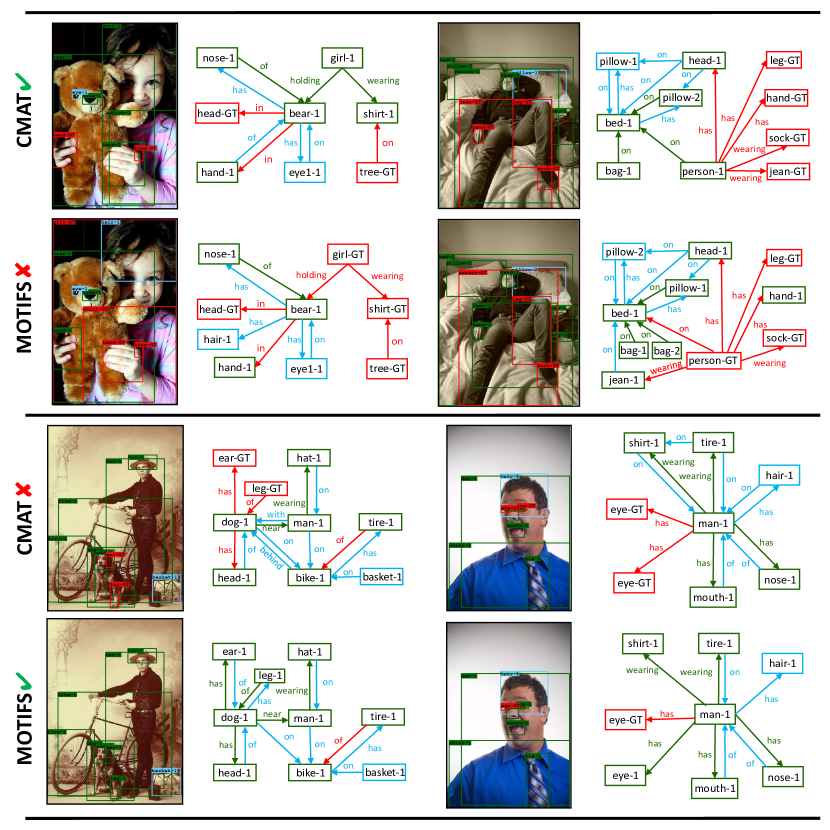
Qualitative Results. Figure 6 shows the qualitative results compared with MOTIFS. From the results in the top two rows, we can observe that CMAT rarely mistakes at the important hub nodes such as the man or girl, because CMAT directly optimizes the graph-coherent objective. From the results in the bottom two rows, the mistakes of CMAT always come from the incomplete annotation of VG: CMAT can detect more false positive (the blue color) objects and relationship than MOTIFS. Since the evaluation metric (i.e., Recall@K) is based on the ranking of labeled triplet confidence, thus, detecting more reasonable false positive results with high confidence will worsen the results.

5 Conclusions

We proposed a novel method CMAT to address the inherent problem with XE based objective in SGG: it is not a graph-coherent objective. CMAT solves the problems by 1) formulating SGG as a multi-agent cooperative task, and using graph-level metrics as the training reward. 2) disentangling the individual contribution of each object to allow a more focused training signal. We validated the effectiveness of CMAT through extensive comparative and ablative experiments. Moving forward, we are going to 1) design a more effective graph-level metric to guide the CMAT training and 2) apply CMAT in downstream tasks such as VQA [61, 70], dialog [41], and captioning [64].

Acknowledgement This work is supported by Zhejiang Natural Science Foundation (LR19F020002, LZ17F020001), National Natural Science Foundation of China (6197020369, 61572431), National Key Research and Development Program of China (SQ2018AAA010010), the Fundamental Research Funds for the Central Universities and Chinese Knowledge Center for Engineering Sciences and Technology. L. Chen is supported by 2018 Zhejiang University Academic Award for Outstanding Doctoral Candidates. H. Zhang is supported by NTU Data Science and Artificial Intelligence Research Center (DSAIR) and NTU-Alibaba Lab.

Appendix

This supplementary document is organized as follows:

• Section A provides the details of some simplified functions in Agent Communication and Visual Relationship Detection.

• Section B provides the detailed proof of the CMAT convergence, which guarantees that the proposed CMAT method can converge to a locally optimal policy.

• Section C provides the detailed derivation of Eq. (6), i.e., $\nabla_{\theta}J\approx\sum^{n}_{i=1}\nabla_{\theta}\log\bm{p}^{T}_{i}(v^{T}_{i}|h^{T}_{i};\theta)Q(H^{T},V^{T})$.

• Section D shows more qualitative results of CMAT compared with the strong baseline MOTIFS [73] in SGDet setting.

Appendix A Details of Some Simplified Functions

We demonstrate the details of some omitted functions in Eq. (1), Eq. (2), Eq. (3) and Eq. (4).

A.1 $F_{s}$ and $F_{e}$ in Extract Module

$$\bm{h}^{t}_{i} =\text{LSTM}(\bm{h}^{t-1}_{i},[\bm{x}^{t}_{i},\bm{e}^{t-1}_{i}]),$$ (11)

$$\bm{s}^{t}_{i} =\bm{s}^{t-1}_{i}+\bm{W}_{h}\bm{h}^{t}_{i},$$

$$v^{t}_{i} \sim\bm{p}^{t}_{i}=\text{softmax}(\bm{s}^{t}_{i}),$$

$$\bm{e}^{t}_{i} =\textstyle{\sum_{\tilde{v}}}\bm{p}^{t}_{i}(\tilde{v})\mathbf{E}[\tilde{v}],$$

where $\bm{h}^{t}_{i}\in\mathbb{R}^{h}$ is the hidden state of LSTM, $\bm{x}^{t}_{i}\in\mathbb{R}^{d}$ is the time-step input feature and $\bm{s}^{t}_{i}\in\mathbb{R}^{|\mathcal{C}|}$ is the object class confidence. $\mathbf{E}[\tilde{v}]\in\mathbb{R}^{e}$ is the embedding of class label $\tilde{v}\in\mathcal{C}$ and $\bm{e}^{t}_{i}\in\mathbb{R}^{e}$ is the soft-weighted embedding of class label based on probabilities $\bm{p}^{t}_{i}$. $\bm{W}_{h}\in\mathbb{R}^{h\times|\mathcal{C}|}$ is a learnable matrix. and $[,]$ is concatenate operation.

A.2 $F_{m*}$ in Message Module

$$\bm{m}^{t}_{j}=\bm{W}_{u}\bm{h}^{t}_{j},\;\bm{m}^{t}_{ij}=\bm{W}_{p}\bm{h}^{t}_{ij}$$ (12)

where $\bm{m}^{t}_{j}\in\mathbb{R}^{h}$ and $\bm{m}^{t}_{ij}\in\mathbb{R}^{h}$ is the unary message and pairwise message, respectively. $\bm{h}^{t}_{ij}\in\bm{R}^{d}$ is the pairwsie feature between agent $i$ and agent $j$. $\bm{W}_{u}\in\mathbb{R}^{h\times h}$, $\bm{W}_{p}\in\mathbb{R}^{d\times h}$ are learnable mapping matrices.

A.3 $F_{att*}$ and $F_{u*}$ in Update Module

$$u^{t}_{j} =\bm{w}_{u}[\bm{h}^{t}_{i},\bm{h}^{t}_{j}],\;\alpha^{t}_{j}=\exp(u^{t}_{j})/\textstyle{\sum_{k}}\exp(u^{t}_{k}),$$ (13)

$$u^{t}_{ij} =\bm{w}_{p}[\bm{h}^{t}_{i},\bm{h}^{t}_{ij}],\;\alpha^{t}_{ij}=\exp(u^{t}_{ij})/\textstyle{\sum_{k}}\exp(u^{t}_{ik})$$

$$\bm{x}^{t+1}_{i} =\bm{W}_{x}(\text{ReLU}(\bm{h}^{t}_{i}+\textstyle{\sum_{j}}\alpha^{t}_{j}\bm{m}^{t}_{j}+\textstyle{\sum_{j}}\alpha^{t}_{ij}\bm{m}^{t}_{ij}))$$

$$\bm{h}^{t+1}_{ij} =\text{ReLU}(\bm{h}^{t}_{ij}+\bm{W}_{s}\bm{h}^{t+1}_{i}+\bm{W}_{e}\bm{h}^{t+1}_{j})$$

where $\alpha^{t}_{j}$ and $\alpha^{t}_{ij}$ are attention weights to fuse different messages, $\bm{w}_{u}\in\mathbb{R}^{2h}$, $\bm{w}_{p}\in\mathbb{R}^{h+d}$, $\bm{W}_{x}\in\mathbb{R}^{h\times d}$, $\bm{W}_{s}\in\mathbb{R}^{h\times d}$, and $\bm{W}_{e}\in\mathbb{R}^{h\times d}$ are learnable mapping matrices.

A.4 $F_{r}$ in Visual Relationship Detection

$$\bm{z}_{i} =\bm{W}_{o}[\bm{h}^{T}_{i},\mathbf{E}[v^{T}_{i}]],\;\bm{z}_{j}=\bm{W}_{o}[\bm{h}^{T}_{j},\mathbf{E}[v^{T}_{j}]],$$ (14)

$$\bm{p}_{ij} =\text{softmax}([\bm{z}_{i},\bm{z}_{j}]\odot\bm{W}_{r}\bm{z}_{ij}+\bm{w}_{v^{T}_{i},v^{T}_{j}}),$$

$$r_{ij} =\arg\textstyle{\max_{r\in\mathcal{R}}}\bm{p}_{ij}(r),$$

where $\bm{W}_{o}\in\mathbb{R}^{(h+e)\times z}$, $\bm{W}_{r}\in\mathbb{R}^{z\times 2z}$ are transformation matrices, $\bm{z}_{ij}\in\mathbb{R}^{z}$ is the predicated visual feature between agent $i$ and $j$, $\odot$ is a fusing function , and $\bm{w}_{v^{T}_{i},v^{T}_{j}}\in\mathbb{R}^{|\mathcal{C}|}$ is the bias vector specific to head and tail labels as in [73].

Predicate Visual Features $z_{ij}$. For the predicate visual features, we used RoIAlign to pool the union box of subject and object, and resized the union box feature to $7\times 7\times 512$. Following [73, 7], we used a $14\times 14\times 2$ binary feature map to model the geometric spatial position of subject and object, with one channel per box. We applied two convolutional layers on this binary feature map and obtained a new $7\times 7\times 512$ spatial position feature map. We added this position feature map with the previous resized union box feature, and applied two fully-connected layers to obtain the final predicate visual feature.

Appendix B Proof of the Convergence of CMAT

Proof.

We denote $\pi_{i}$ as the policy of agent $i$, i.e.,$\pi_{i}=\bm{p}^{T}_{i}$ and $\bm{\pi}$ as the joint policy of all agents, i.e., $\bm{\pi}=\{\bm{p}^{T}_{1},...,\bm{p}^{T}_{n}\}$. Then, the expected gradient of CMAT is given by (cf. Eq. (11)):

$$\nabla_{\theta}J =\mathbb{E}_{\bm{\pi}}\left[\sum^{n}_{i=1}\nabla_{\theta}\log\pi_{i}(v^{T}_{i})A^{i}(H^{T},V^{T})\right],$$ (15)

$$=\mathbb{E}_{\bm{\pi}}\left[\sum^{n}_{i=1}\nabla_{\theta}\log\pi_{i}(v^{T}_{i})(R(H^{T},V^{T})-b(H^{T},V^{T}_{-i}))\right].$$

where the expection $\mathbb{E}_{\bm{\pi}}$ is with respect to the state-action distribution induced by the joint policy $\bm{\pi}$, $b(H^{T},V^{T}_{-i})$ is the counterfactual baseline in CMAT model, i.e., $b(H^{T},V^{T}_{-i})=\sum\bm{p}^{T}_{i}(\tilde{v}^{T}_{i})R(H^{T},(V^{T}_{-i},\tilde{v}^{T}_{i})).$

First, consider the expected contribution of this counterfactual baseline $b(H^{T},V^{T}_{-i})$,

$$\nabla_{\theta}J_{b}=\mathbb{E}_{\bm{\pi}}\left[\sum^{n}_{i=1}\nabla_{\theta}\log\pi_{i}(v^{T}_{i})b(H^{T},V^{T}_{-i})\right].$$ (16)

Let $d^{\bm{\pi}}(s)$ be the discounted ergodic state distribution as defined by  [56]:

$$\nabla_{\theta}J_{b}= \sum_{s}d^{\bm{\pi}}(s)\sum^{n}_{i=1}\sum_{V^{T}_{-i}}\bm{\pi}(V^{T}_{-i})\sum_{v^{T}_{i}}\pi_{i}(v^{T}_{i})\nabla_{\theta}\log\pi_{i}(v^{T}_{i})b(H^{T},V^{T}_{-i})$$ (17)

$$= \sum_{s}d^{\bm{\pi}}(s)\sum^{n}_{i=1}\sum_{V^{T}_{-i}}\bm{\pi}(V^{T}_{-i})\sum_{v^{T}_{i}}\nabla_{\theta}\pi_{i}(v^{T}_{i})b(H^{T},V^{T}_{-i})$$

$$= \sum_{s}d^{\bm{\pi}}(s)\sum^{n}_{i=1}\sum_{V^{T}_{-i}}\bm{\pi}(V^{T}_{-i})b(H^{T},V^{T}_{-i})\nabla_{\theta}1$$

$$= 0$$

Thus, this counterfactual baseline does not change the expected gradient. The reminder of the expected policy gradient is given by:

$$\nabla_{\theta}J =\mathbb{E}_{\bm{\pi}}\left[\sum^{n}_{i=1}\nabla_{\theta}\log\pi_{i}(v^{T}_{i})R(H^{T},V^{T})\right],$$ (18)

$$=\mathbb{E}_{\bm{\pi}}\left[\nabla_{\theta}\log\prod^{n}_{i=1}\pi_{i}(v^{T}_{i})R(H^{T},V^{T})\right].$$ (19)

Writing the joint policy into a product of the independent policies:

$$\bm{\pi}(V^{T})=\prod^{n}_{i=1}\pi_{i}(v^{T}_{i}),$$ (20)

we have the standard single-agent policy gradient:

$$\nabla_{\theta}J=\mathbb{E}_{\bm{\pi}}\left[\nabla_{\theta}\log\bm{\pi}(V^{T})R(H^{T},V^{T})\right].$$ (21)

Konda et al. [25] proved that this gradient converges to a local maximum of the expected return $J$, given that: 1) the policy $\bm{\pi}$ is differentiable, 2) the update timescales for $\bm{\pi}$ are sufficiently slow. Meanwhile, the parameterization of the policy (i.e., the single-agent joint-action learner is decomposed into independent policies) is immaterial to convergence, as long as it remains differentiable. ∎

Appendix C Derivation of Eq. (6)

Based on the policy gradient theorem we provide the detailed derivation of Eq. (6) as follows. We denote the action sequence for agent $i$ as $\hat{A}_{i}=\{\hat{a}^{1}_{i},\hat{a}^{2}_{i},...,\hat{a}^{T}_{i}\}$, and value function $V_{\theta}(\hat{A}_{i})$ as the expected future reward of sequence $\hat{A}_{i}$. Then the gradient of agent $i$ is:

$$\nabla_{\theta}J_{i} =\frac{dV(\hat{A}_{i})}{d\theta}=\frac{d}{d\theta}\mathbb{E}_{\hat{A}_{i}\sim\pi^{t}_{i}(\hat{A}_{i})}R(\hat{A}_{i})$$ (22)

$$=\sum_{\hat{A}_{i}}\frac{d}{d\theta}\left[\pi^{t}_{i}(\hat{a}^{1}_{i})\pi^{t}_{i}(\hat{a}^{2}_{i}|\hat{a}^{1}_{i})..\pi^{t}_{i}(\hat{a}^{T}_{i}|\hat{a}^{1}_{i}..\hat{a}^{T-1}_{i})\right]R(\hat{A}_{i})$$

$$=\sum^{T}_{t=1}\sum_{\hat{A}_{i}}\pi^{t}_{i}(\hat{A}^{1..t-1}_{i})\frac{d\pi^{t}_{i}(\hat{a}^{t}_{i}|\hat{A}^{1..t-1}_{i})}{d\theta}\pi^{t}_{i}(\hat{A}^{t+1..T}_{i}|\hat{A}^{1..t}_{i})R(\hat{A}_{i})$$

$$=\sum^{T}_{t=1}\sum_{\hat{A}^{1..t}_{i}}\pi^{t}_{i}(\hat{A}^{1..t-1}_{i})\frac{\pi^{t}_{i}(\hat{a}^{t}_{i}|\hat{A}^{1..t-1}_{i})}{d\theta}\sum_{\hat{A}^{t+1..T}_{i}}\pi^{t}_{i}(\hat{A}^{t+1..T}_{i}|\hat{A}^{1..t}_{i})\sum^{T}_{\tau=1}r^{\tau}_{i}(\hat{a}^{\tau}_{i};\hat{A}^{1..\tau-1}_{i})$$

$$=\sum^{T}_{t=1}\sum_{\hat{A}^{1..t}_{i}}\pi^{t}_{i}(\hat{A}^{1..t-1}_{i})\frac{\pi^{t}_{i}(\hat{a}^{t}_{i}|\hat{A}^{1..t-1}_{i})}{d\theta}\left[r^{t}(\hat{a}^{t}_{i};\hat{A}^{1..t-1}_{i})+\sum_{\hat{A}^{t+1..T}_{i}}\pi^{t}_{i}(\hat{Y}^{t+1..T}_{i}|\hat{Y}^{1..t}_{i})\sum^{T}_{\tau=t+1}r^{\tau}_{i}(\hat{a}^{\tau}_{i};\hat{A}^{1..\tau-1}_{i})\right]$$

$$=\sum^{T}_{t=1}\mathbb{E}_{\hat{A}^{1..t-1}_{i}\sim\pi^{t}_{i}(\hat{A}^{1..t-1}_{i})}\sum_{a^{t}\in\mathcal{A}}\frac{d\pi^{t}_{i}(a^{t}|\hat{A}^{1..t-1}_{i})}{d\theta}Q(a^{t};\hat{A}^{1..t-1}_{i})$$

$$=\mathbb{E}_{\hat{A}_{i}\sim\pi^{t}_{i}(\hat{A}_{i})}\sum^{T}_{t=1}\sum_{a^{t}\in\mathcal{A}}\frac{\pi^{t}_{i}(a^{t}|\hat{A}^{1..t-1}_{i})}{d\theta}Q(a^{t};\hat{A}^{1..t-1}_{i})$$

Further, the gradient for agent $i$ can be simplified as:

$$\nabla_{\theta}J_{i} =\mathbb{E}\left[\sum^{T}_{t=1}\sum_{a^{t}_{i}\in\mathcal{A}}\nabla_{\theta}\pi^{t}_{i}(a^{t}_{i})Q(s^{t}_{i},a^{t}_{i})\right]$$ (23)

$$=\mathbb{E}\left[\sum^{T}_{t=1}\sum_{a^{t}_{i}\in\mathcal{A}}\pi^{t}_{i}(a^{t}_{i})\nabla_{\theta}\log\pi^{t}_{i}(a^{t}_{i})Q(s^{t}_{i},a^{t}_{i})\right]$$

$$\approx\sum^{T}_{t=1}\nabla_{\theta}\log\pi^{t}_{i}(a^{t}_{i})Q(s^{t}_{i},a^{t}_{i})$$

Therefore, for the time step $t$, the gradient for agent $i$ is $\nabla_{\theta}\log\pi^{t}_{i}(a^{t}_{i})Q(s^{t}_{i},a^{t}_{i})$. For multi-agent in a cooperative environment, the state-action function $Q$ should estimate the reward based on the set of all agent state and actions, i.e., $Q(S^{t},A^{t})$. Then, the gradient for all agents is:

$$\nabla_{\theta}J\approx\sum^{n}_{i=1}\nabla_{\theta}J_{i}=\sum^{n}_{i=1}\nabla_{\theta}\log\pi^{t}_{i}(a^{t}_{i}|s^{t}_{i})Q(S^{t},A^{t}).$$ (24)

In our CMAT, we CMAT samples actions after $T$-round agent communication, and the action for agent $i$ is $\bm{v}^{T}_{i}$, the policy function is $\bm{p}^{T}_{i}$, and the state of agent is $\bm{h}^{t}$, i.e., $S^{t}=H^{t},A^{t}=V^{t}$. Therefore, the gradient for the cooperative multi-agent in CMAT is:

$$\nabla_{\theta}J\approx\sum^{n}_{i=1}\nabla_{\theta}\log\bm{p}^{T}_{i}(v^{T}_{i}|h^{T}_{i};\theta)Q(H^{T},V^{T})$$ (25)

Appendix D More Qualitative Results

Figure 7 and 8 show more qualitative results of CMAT and MOTIFS in SGDet setting. From the rows where CMAT is better than MOTIFS, we can see that CMAT rarely mistakes at the important hub nodes such aas the “surfboard” or “laptop”. This is because CMAT directly optimizes the graph-coherent objective. However, the rows show that the mistakes made by CMAT always come from the imcomplete anntation of CMAT can detect more false positive (the blue color) objects and relationship than MOTIFS. Since the evaluation metric (i.e., Recall@K) is based on the ranking of labeled triplet confidence, thus, detecting more reasonable false positive results with high confidence can worsen the performance.

Figure 7: More qualitative results showing comparisons between CMAT and MOTIFS in the SGDet setting. Green boxes are detected boxes with IoU large 0.5 with the ground truth, blue boxes are detected but not labeled, red boxes are ground-truth with no match. Green edges are true positive predicted by each model at the R@20 setting, red edges are false negatives, and blue edges are false positives. Only detected boxes overlapped with ground-truth are shown.

Figure 8: The caption is same as the one in Figure 8. More qualitative results showing comparisons between CMAT and MOTIFS in the SGDet setting. Green boxes are detected boxes with IoU large 0.5 with the ground truth, blue boxes are detected but not labeled, red boxes are ground-truth with no match. Green edges are true positive predicted by each model at the R@20 setting, red edges are false negatives, and blue edges are false positives. Only detected boxes overlapped with ground-truth are shown.

References

- [1] Peter Anderson, Basura Fernando, Mark Johnson, and Stephen Gould. Spice: Semantic propositional image caption evaluation. In ECCV, 2016.
- [2] Dzmitry Bahdanau, Philemon Brakel, Kelvin Xu, Anirudh Goyal, Ryan Lowe, Joelle Pineau, Aaron Courville, and Yoshua Bengio. An actor-critic algorithm for sequence prediction. In ICLR, 2017.
- [3] Juan C Caicedo and Svetlana Lazebnik. Active object localization with deep reinforcement learning. In ICCV, 2015.
- [4] Kan Chen, Rama Kovvuri, and Ram Nevatia. Query-guided regression network with context policy for phrase grounding. In ICCV, 2017.
- [5] Long Chen, Hanwang Zhang, Jun Xiao, Liqiang Nie, Jian Shao, Wei Liu, and Tat-Seng Chua. Sca-cnn: Spatial and channel-wise attention in convolutional networks for image captioning. In CVPR, 2017.
- [6] Tianshui Chen, Weihao Yu, Riquan Chen, and Liang Lin. Knowledge-embedded routing network for scene graph generation. In CVPR, 2019.
- [7] Bo Dai, Yuqi Zhang, and Dahua Lin. Detecting visual relationships with deep relational networks. In CVPR, 2017.
- [8] Abhishek Das, Satwik Kottur, José MF Moura, Stefan Lee, and Dhruv Batra. Learning cooperative visual dialog agents with deep reinforcement learning. In ICCV, 2017.
- [9] Santosh K Divvala, Derek Hoiem, James H Hays, Alexei A Efros, and Martial Hebert. An empirical study of context in object detection. In CVPR, 2009.
- [10] Jakob Foerster, Ioannis Alexandros Assael, Nando de Freitas, and Shimon Whiteson. Learning to communicate with deep multi-agent reinforcement learning. In NeurIPS, 2016.
- [11] Jakob Foerster, Gregory Farquhar, Triantafyllos Afouras, Nantas Nardelli, and Shimon Whiteson. Counterfactual multi-agent policy gradients. In AAAI, 2018.
- [12] Jakob Foerster, Nantas Nardelli, Gregory Farquhar, Triantafyllos Afouras, Philip HS Torr, Pushmeet Kohli, and Shimon Whiteson. Stabilising experience replay for deep multi-agent reinforcement learning. In ICML, 2017.
- [13] Jiuxiang Gu, Handong Zhao, Zhe Lin, Sheng Li, Jianfei Cai, and Mingyang Ling. Scene graph generation with external knowledge and image reconstruction. In CVPR, 2019.
- [14] Monica Haurilet, Alina Roitberg, and Rainer Stiefelhagen. It’s not about the journey; it’s about the destination: Following soft paths under question-guidance for visual reasoning. In CVPR, 2019.
- [15] Matthew Hausknecht and Peter Stone. Deep recurrent q-learning for partially observable mdps. In AAAI, 2015.
- [16] Kaiming He, Georgia Gkioxari, Piotr Dollár, and Ross Girshick. Mask r-cnn. In ICCV, 2017.
- [17] Roei Herzig, Moshiko Raboh, Gal Chechik, Jonathan Berant, and Amir Globerson. Mapping images to scene graphs with permutation-invariant structured prediction. In NeurIPS, 2018.
- [18] Ronghang Hu, Jacob Andreas, Marcus Rohrbach, Trevor Darrell, and Kate Saenko. Learning to reason: End-to-end module networks for visual question answering. In ICCV, 2017.
- [19] Drew A Hudson and Christopher D Manning. Gqa: A new dataset for real-world visual reasoning and compositional question answering. In CVPR, 2019.
- [20] Seong Jae Hwang, Sathya N Ravi, Zirui Tao, Hyunwoo J Kim, Maxwell D Collins, and Vikas Singh. Tensorize, factorize and regularize: Robust visual relationship learning. In CVPR, 2018.
- [21] Zequn Jie, Xiaodan Liang, Jiashi Feng, Xiaojie Jin, Wen Lu, and Shuicheng Yan. Tree-structured reinforcement learning for sequential object localization. In NeurIPS, 2016.
- [22] Justin Johnson, Bharath Hariharan, Laurens van der Maaten, Judy Hoffman, Li Fei-Fei, C Lawrence Zitnick, and Ross B Girshick. Inferring and executing programs for visual reasoning. In ICCV, 2017.
- [23] Justin Johnson, Ranjay Krishna, Michael Stark, Li-Jia Li, David Shamma, Michael Bernstein, and Li Fei-Fei. Image retrieval using scene graphs. In CVPR, 2015.
- [24] Dong-Jin Kim, Jinsoo Choi, Tae-Hyun Oh, and In So Kweon. Dense relational captioning: Triple-stream networks for relationship-based captioning. In CVPR, 2019.
- [25] Vijay R Konda and John N Tsitsiklis. Actor-critic algorithms. In NeurIPS, 2000.
- [26] Philipp Krähenbühl and Vladlen Koltun. Efficient inference in fully connected crfs with gaussian edge potentials. In NeurIPS, 2011.
- [27] Ranjay Krishna, Yuke Zhu, Oliver Groth, Justin Johnson, Kenji Hata, Joshua Kravitz, Stephanie Chen, Yannis Kalantidis, Li-Jia Li, David A Shamma, et al. Visual genome: Connecting language and vision using crowdsourced dense image annotations. IJCV, 2017.
- [28] Yikang Li, Wanli Ouyang, Xiaogang Wang, and Xiao’ou Tang. Vip-cnn: Visual phrase guided convolutional neural network. In CVPR, 2017.
- [29] Yikang Li, Wanli Ouyang, Bolei Zhou, Yawen Cui, Jianping Shi, and Xiaogang Wang. Factorizable net: An efficient subgraph-based framework for scene graph generation. In ECCV, 2018.
- [30] Yikang Li, Wanli Ouyang, Bolei Zhou, Kun Wang, and Xiaogang Wang. Scene graph generation from objects, phrases and region captions. In ICCV, 2017.
- [31] Xiaodan Liang, Lisa Lee, and Eric P Xing. Deep variation-structured reinforcement learning for visual relationship and attribute detection. In CVPR, 2017.
- [32] Daqing Liu, Zheng-Jun Zha, Hanwang Zhang, Yongdong Zhang, and Feng Wu. Context-aware visual policy network for sequence-level image captioning. In ACM MM, 2018.
- [33] Siqi Liu, Zhenhai Zhu, Ning Ye, Sergio Guadarrama, and Kevin Murphy. Improved image captioning via policy gradient optimization of spider. In ICCV, 2017.
- [34] Wei Liu, Dragomir Anguelov, Dumitru Erhan, Christian Szegedy, Scott Reed, Cheng-Yang Fu, and Alexander C Berg. Ssd: Single shot multibox detector. In ECCV, 2016.
- [35] Jonathan Long, Evan Shelhamer, and Trevor Darrell. Fully convolutional networks for semantic segmentation. In CVPR, 2015.
- [36] Ryan Lowe, Yi Wu, Aviv Tamar, Jean Harb, OpenAI Pieter Abbeel, and Igor Mordatch. Multi-agent actor-critic for mixed cooperative-competitive environments. In NeurIPS, 2017.
- [37] Cewu Lu, Ranjay Krishna, Michael Bernstein, and Li Fei-Fei. Visual relationship detection with language priors. In ECCV, 2016.
- [38] Stefan Mathe, Aleksis Pirinen, and Cristian Sminchisescu. Reinforcement learning for visual object detection. In CVPR, 2016.
- [39] Volodymyr Mnih, Adria Puigdomenech Badia, Mehdi Mirza, Alex Graves, Timothy Lillicrap, Tim Harley, David Silver, and Koray Kavukcuoglu. Asynchronous methods for deep reinforcement learning. In ICML, 2016.
- [40] Alejandro Newell and Jia Deng. Pixels to graphs by associative embedding. In NeurIPS, 2017.
- [41] Yulei Niu, Hanwang Zhang, Manli Zhang, Jianhong Zhang, Zhiwu Lu, and Ji-Rong Wen. Recursive visual attention in visual dialog. In CVPR, 2019.
- [42] Will Norcliffe-Brown, Stathis Vafeias, and Sarah Parisot. Learning conditioned graph structures for interpretable visual question answering. In NeurIPS, 2018.
- [43] Shayegan Omidshafiei, Jason Pazis, Christopher Amato, Jonathan P How, and John Vian. Deep decentralized multi-task multi-agent reinforcement learning under partial observability. In ICML, 2017.
- [44] Mengshi Qi, Weijian Li, Zhengyuan Yang, Yunhong Wang, and Jiebo Luo. Attentive relational networks for mapping images to scene graphs. In CVPR, 2019.
- [45] Xufeng Qian, Yueting Zhuang, Yimeng Li, Shaoning Xiao, Shiliang Pu, and Jun Xiao. Video relation detection with spatio-temporal graph. In ACM MM, 2019.
- [46] Marc’Aurelio Ranzato, Sumit Chopra, Michael Auli, and Wojciech Zaremba. Sequence level training with recurrent neural networks. In ICLR, 2016.
- [47] Yongming Rao, Dahua Lin, Jiwen Lu, and Jie Zhou. Learning globally optimized object detector via policy gradient. In CVPR, 2018.
- [48] Joseph Redmon and Ali Farhadi. Yolo9000: better, faster, stronger. In CVPR, 2017.
- [49] Shaoqing Ren, Kaiming He, Ross Girshick, and Jian Sun. Faster r-cnn: Towards real-time object detection with region proposal networks. In NeurIPS, 2015.
- [50] Zhou Ren, Xiaoyu Wang, Ning Zhang, Xutao Lv, and Li-Jia Li. Deep reinforcement learning-based image captioning with embedding reward. In CVPR, 2017.
- [51] Steven J Rennie, Etienne Marcheret, Youssef Mroueh, Jarret Ross, and Vaibhava Goel. Self-critical sequence training for image captioning. In CVPR, 2017.
- [52] Xindi Shang, Tongwei Ren, Jingfan Guo, Hanwang Zhang, and Tat-Seng Chua. Video visual relation detection. In ACM MM, 2017.
- [53] Jiaxin Shi, Hanwang Zhang, and Juanzi Li. Explainable and explicit visual reasoning over scene graphs. In CVPR, 2019.
- [54] Karen Simonyan and Andrew Zisserman. Very deep convolutional networks for large-scale image recognition. In ICLR, 2015.
- [55] Richard S Sutton, Andrew G Barto, Francis Bach, et al. Reinforcement learning: An introduction. MIT press, 1998.
- [56] Richard S Sutton, David A McAllester, Satinder P Singh, and Yishay Mansour. Policy gradient methods for reinforcement learning with function approximation. In NeurIPS, 2000.
- [57] Ardi Tampuu, Tambet Matiisen, Dorian Kodelja, Ilya Kuzovkin, Kristjan Korjus, Juhan Aru, Jaan Aru, and Raul Vicente. Multiagent cooperation and competition with deep reinforcement learning. In arXiv, 2015.
- [58] Kaihua Tang, Hanwang Zhang, Baoyuan Wu, Wenhan Luo, and Wei Liu. Learning to compose dynamic tree structures for visual contexts. In CVPR, 2019.
- [59] Wenbin Wang, Ruiping Wang, Shiguang Shan, and Xilin Chen. Exploring context and visual pattern of relationship for scene graph generation. In CVPR, 2019.
- [60] Lex Weaver and Nigel Tao. The optimal reward baseline for gradient-based reinforcement learning. In UAI, 2001.
- [61] Dejing Xu, Zhou Zhao, Jun Xiao, Fei Wu, Hanwang Zhang, Xiangnan He, and Yueting Zhuang. Video question answering via gradually refined attention over appearance and motion. In ACM MM, 2017.
- [62] Danfei Xu, Yuke Zhu, Christopher B Choy, and Li Fei-Fei. Scene graph generation by iterative message passing. In CVPR, 2017.
- [63] Kelvin Xu, Jimmy Ba, Ryan Kiros, Kyunghyun Cho, Aaron Courville, Ruslan Salakhudinov, Rich Zemel, and Yoshua Bengio. Show, attend and tell: Neural image caption generation with visual attention. In ICML, 2015.
- [64] Ning Xu, An-An Liu, Yongkang Wong, Yongdong Zhang, Weizhi Nie, Yuting Su, and Mohan Kankanhalli. Dual-stream recurrent neural network for video captioning. CSVT, 2018.
- [65] Jianwei Yang, Jiasen Lu, Stefan Lee, Dhruv Batra, and Devi Parikh. Graph r-cnn for scene graph generation. In ECCV, 2018.
- [66] Xu Yang, Kaihua Tang, Hanwang Zhang, and Jianfei Cai. Auto-encoding scene graphs for image captioning. In CVPR, 2019.
- [67] Xu Yang, Hanwang Zhang, and Jianfei Cai. Shuffle-then-assemble: learning object-agnostic visual relationship features. In ECCV, 2018.
- [68] Xu Yang, Hanwang Zhang, and Jianfei Cai. Learning to collocate neural modules for image captioning. In ICCV, 2019.
- [69] Ting Yao, Yingwei Pan, Yehao Li, and Tao Mei. Exploring visual relationship for image captioning. In ECCV, 2018.
- [70] Yunan Ye, Zhou Zhao, Yimeng Li, Long Chen, Jun Xiao, and Yueting Zhuang. Video question answering via attribute-augmented attention network learning. In SIGIR, 2017.
- [71] Guojun Yin, Lu Sheng, Bin Liu, Nenghai Yu, Xiaogang Wang, Jing Shao, and Chen Change Loy. Zoom-net: Mining deep feature interactions for visual relationship recognition. In ECCV, 2018.
- [72] Licheng Yu, Hao Tan, Mohit Bansal, and Tamara L Berg. A joint speakerlistener-reinforcer model for referring expressions. In CVPR, 2017.
- [73] Rowan Zellers, Mark Yatskar, Sam Thomson, and Yejin Choi. Neural motifs: Scene graph parsing with global context. In CVPR, 2018.
- [74] Hanwang Zhang, Zawlin Kyaw, Shih-Fu Chang, and Tat-Seng Chua. Visual translation embedding network for visual relation detection. In CVPR, 2017.
- [75] Ji Zhang, Mohamed Elhoseiny, Scott Cohen, Walter Chang, and Ahmed Elgammal. Relationship proposal networks. In CVPR, 2017.
- [76] Ji Zhang, Kevin J. Shih, Ahmed Elgammal, Andrew Tao, and Bryan Catanzaro. Graphical contrastive losses for scene graph parsing. In CVPR, 2019.
- [77] Li Zhang, Flood Sung, Feng Liu, Tao Xiang, Shaogang Gong, Yongxin Yang, and Timothy M Hospedales. Actor-critic sequence training for image captioning. In NeurIPS Workshop, 2017.
- [78] Yan Zhang, Jonathon Hare, and Adam Prügel-Bennett. Learning to count objects in natural images for visual question answering. In ICLR, 2018.
- [79] Shuai Zheng, Sadeep Jayasumana, Bernardino Romera-Paredes, Vibhav Vineet, Zhizhong Su, Dalong Du, Chang Huang, and Philip HS Torr. Conditional random fields as recurrent neural networks. In ICCV, 2015.
- [80] Yaohui Zhu and Shuqiang Jiang. Deep structured learning for visual relationship detection. In AAAI, 2018.
- [81] Bohan Zhuang, Lingqiao Liu, Chunhua Shen, and Ian Reid. Towards context-aware interaction recognition for visual relationship detection. In ICCV, 2017.