Towards a Fisher-information description of complexity in de Sitter universe

Abstract

Abstract

Recent developments on holography and quantum information physics suggest that quantum information theory has come to play a fundamental role in understanding quantum gravity. Cosmology, on the other hand, plays a significant role in testing quantum gravity effects. How to apply this idea to a realistic universe is still unknown. Here, we show that some concepts in quantum information theory have cosmological descriptions. Particularly, we show that the complexity of a tensor network can be regarded as a Fisher information measure (FIM) of a dS universe, followed by several observations: (i) the holographic entanglement entropy has a tensor-network description and admits a information-theoretical interpretation, (ii) on-shell action of dS spacetime has a same description of FIM, (iii) complexity/action(CA) duality holds for dS spacetime. Our result is also valid for $f(R)$ gravity, whose FIM exhibits the same features of a recent proposed $L^{n}$ norm complexity.

I Introduction

A milestone in the exploration of the unification of general relativity and quantum mechanics was the work of Bekenstein and Hawking on the area law of black hole entropy Bekenstein:1973ur ; Hawking:1974rv . Inspired by this discovery, ’t Hooft tHooft:1993dmi and Susskind Susskind:1994vu formulated the holographic principle, which suggests that the degrees of freedom of a higher dimensional gravitational system can be characterized by those of a lower dimensional quantum system. This principle is currently widely regarded as a fundamental principle of quantum gravity, especially after Maldacena’s discovery Maldacena:1997re ; Witten:1998 of AdS(Anti-de Sitter)/CFT(Conformal field theory) correspondence.

However, how these extra degrees of freedom emerge from CFT is still a mystery. A breakthrough came from the recently proposed holographic entanglement entropy (HEE) Ryu:2006bv , which suggests deep connections between quantum gravity theory and quantum information theory VanRaamsdonk:2010pw ; Swingle:2009bg . However, although these connections are generally believed to grasp a significant character of the theory of quantum gravity, there is a lack of applications to the realistic universe. Most current achievements are valid only for AdS spacetimes, with very limited efforts to our realistic universe.

In this work, we try to make a preliminary attempt to cross these gaps. We focus on the possible relations between the Friedmann-Robertson-Walker (FRW) universe (particularly the dS universe) and quantum information theory. We show that complexity of a multi-scale entanglement renormalization ansatz (MERA) Vidal:2008zz tensor network can be thought of as FIM of a dS spacetime. Our argument is based on the following three observations: First, we will show that for MERA tensor network, the entanglement entropy of a cut leg can be viewed as a flow—an information-bit (qubit) flow transmitted by a quantum circuit. It provides an information-theoretical picture of the MERA network. According to this picture, tensor network and spacetimes admit the same causal structure. This is consistent with the MERA/spacetime correspondence proposed in Beny:2011vh , where MERA is regarded as a quantum circuit and the dS metric is derived. A similar perspective can be found in Czech:2015qta ; Czech:2015kbp ; Asplund:2016koz ; Czech:2016xec ; deBoer:2015kda , where MERA is viewed as a discretization of kinematic space—the space of bulk geodesics, instead of the time slice of the original bulk, and the kinematic space of an AdS space is of dS geometry. Second, the on-shell action of dS can be identified as an FIM, which is a description of the measure of information. Third, we show that the on-shell Einstein-Hilbert (EH) action of dS spacetime exhibits the same features as complexity of MERA network, which can be viewed as a dS-version complexity/action(CA) duality Brown:2015bva ; Brown:2015lvg ; Chapman:2016hwi ; Carmi:2016wjl . Originally, the CA duality refers to the Wheeler-De Witt(WDW) patch under asymptotic AdS spacetime. In our dS-version CA duality, we do not need to constrain in the WDW patch. This follows from recent generalization, for instance, complexity of MERA in terms of Liouville action as shown in Caputa:2017urj ; Caputa:2017yrh ; Czech:2017ryf ; Caputa:2017 , and dS spacetime as shown in Bao:2017qmt .

II MERA/de Sitter Correspondence

Given a MERA network, without loss of generality, we assume it is a 2-isometry tensor network, which means each isometry in the network has two lower legs and one upper leg. Cutting one leg will gives $\log_{2}\chi$ entropy Vidal:2008zz , where $\chi$ is the bond dimension. The key point is that 2-isometry is a coarse-graining operator mapping $\chi^{2}$-dimensional Hilbert space to $\chi$-dimensional one as illustrated in Figure 1a. This property suggests that $\log_{2}\chi$ can be regarded as flux of entanglement flow in each leg and causal relation between tensors can be viewed as causal structure of the emergent spacetime Swingle:2009bg ; Czech:2015kbp . The entanglement entropy is given by counting the number of legs on the causal cut. Before discussing this MEAR/spacetime correspondence, let us first give a quick snapshot of tensor network in terms of the kinematic space of AdS₃. According to Czech:2015qta ; Czech:2015kbp ; Asplund:2016koz ; Czech:2016xec ; deBoer:2015kda , MERA tensor network is best viewed as kinematic space of AdS₃ rather than the time slice of the original AdS₃. The kinematic space is defined by a set of boundary-anchored geodesics. The measure of a kinematic space is determined by Czech:2015qta ; Asplund:2016koz $\mathcal{D}g\propto(\partial^{2}S(u,v)/\partial u\partial v)dudv$, which is the measure of dS₂.

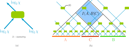
Figure 1: (a) A $2-$isometry tensor element. (b) The multi-scale entanglement renormalization ansatz (MERA) network. We have ignored disentangler because the spacetime volume is only interpreted as conditional mutual information. $A$ and $B$ share the information $I(A,B|C)$ Czech:2015kbp . These entangled degrees of freedom are transmitted by isometry in the blue region.

In terms of this picture, the volume of a causal diamond $D$ can be explained as conditional mutual information of two intervals as shown in Figure 1b: $I(A:B|C)=S(u-du,v)+S(u,v+dv)-S(u,v)-S(u-du,v+dv)=(\partial^{2}S(u,v)/\partial u\partial v)dudv.$ In other words, isometries in the region $D$ share the information of $A$ and $B$ so they contain the entanglement degrees of freedom between $A$ and $B$. The number of information bits in the region $D$, which is denoted as $\mathcal{N}$, is proportional to the volume integral over $D$,

$$\mathcal{N}=\int_{D}d^{2}x\sqrt{-g}\Theta_{I},$$ (1)

where $\Theta_{I}$ is a constant and $g_{\mu\nu}$ is the dS₂ metric with radius $L$. The idea that measuring the volume of a region in a manifold is replaced by counting the number of elements in this region, was first suggested by Riemann Riemann . This is also the main idea of some quantum gravity models such as causal sets theory Bombelli:1987aa and dS/MERA correspondence Beny:2011vh ; Czech:2015qta ; Czech:2015kbp ; SinaiKunkolienkar:2016lgg ; Bao:2017qmt .

Note that the number of information bits in the diamond $D$ (1) of the kinematic space is the same as the conditional mutual information, i.e., $I=\mathcal{N}$. Comparing with (1) and the expression of the conditional mutual information, one immediately has $\Theta_{I}\propto\frac{c}{L^{D}}$, where $c$ is the central charge of the boundary system. This constant can be explained as the “density” of each isometry tensor. It counts the number of information bits (or entangled pairs) in each isometry. In Section IV, we can see that one outstanding improvement in this paper is that we do not identify the number of the isometry as the volume, but rather the on-shell action, because (1) is equivalent to the number of quantum gates acting on an entangled pair in MERA. When $\Theta_{I}$ is a constant, the on-shell action is proportional to the volume, then our statement reduces to the usual one as mentioned above.

Now we treat the (continuous) MERA as a dS geometry rather than the AdS time slice. This implies the emergent dimension is temporal rather than spatial. That means the opposite direction of coarse graining can be viewed as the evolution time $\tau$ of the universe. We can write down the FRW metric for this tensor network

$$ds^{2}_{\text{TN}}=-d\tau^{2}+a^{2}(\tau)d{\bf x}^{2}.$$ (2)

For dS one has $a=\exp(\tau/L)$, where $L$ is the dS radius. One should note that our proposal can be applied to general $D$-dimensional case. Actually, since kinematic space is just an auxiliary space, it is possible to go beyond kinematic space picture to set up the connections between tensor networks and spacetime structure (2), and to discuss this model in cosmology.

III Fisher Information Measure = Gravitational Action

As explained above, the number of isometric tensors can be given by the integral (1). In this section we show that the integral (1) can be regarded as the on-shell action in dS background, with the help of an observation that the on-shell action of dS spacetime can be viewed as a FIM Chimento:2002 .

We can even consider a more general $D$-dimensional spacetime. For a $D$-dimensional spacetime without matter, the total action is given by

$$I_{\text{G}}=\frac{1}{16\pi G_{D}}\int_{\mathcal{M}}d^{D}x\sqrt{-g}(R-2\Lambda)+I_{GHY},$$ (3)

where the first term is the EH action and the second is the Gibbons-Hawking-York (GHY) boundary term. $R$ is the Ricci curvature, $\Lambda=\frac{D-2}{2D}R$ is the cosmological constant and $G_{D}$ is the $D$-dimensional gravitational constant. For $D$-dimension FRW metric (2), the Ricci curvature is $R=2(D-1)\frac{\ddot{a}}{a}+(D-1)(D-2)\frac{\dot{a}^{2}}{a^{2}}$. Particularly, We consider the on-shell action (3) for dS. The Gibbons-Hawking-York boundary terms, which are used to supplement the action so that the variational principle is well-defined, are given by the extrinsic curvature of the boundary surface $\partial\mathcal{M}$ of the spacetime $\mathcal{M}$. In general this term reads

$$I_{GHY}=\frac{1}{8\pi G_{D}}\int_{\partial\mathcal{M}}d^{D-1}x\epsilon\sqrt{h}K,$$ (4)

where $K$ is the trace of extrinsic curvature of the boundary and $h_{ij}=a^{2}\delta_{ij}$ is the induced metric. $\epsilon$ is equal to $+1$ ($-1$) if $\partial\mathcal{M}$ is timelike (spacelike). The boundaries of the dS spacetimes are the spacelike $\tau$ time slices at $\tau_{i}$ and $\tau_{f}$, with outward pointing unit normal $n^{\mu}$ and $n_{\mu}n^{\mu}=\epsilon=-1$. In the FRW metric we have $n^{\mu}=(1,\bf{0})$ at $\tau_{f}$ and $n^{\mu}=(-1,\bf{0})$ at $\tau_{i}$. The trace of extrinsic curvature is given by

$$K=\nabla_{\mu}n^{\mu}=h^{\alpha\beta}\left(\partial_{\beta}n_{\alpha}-\Gamma^{\gamma}_{\alpha\beta}n_{\gamma}\right)=(D-1)\frac{\dot{a}}{a}$$ (5)

The GHY boundary term for the $\tau=\tau_{f}$ slice is obtained

$$I^{(f)}_{GHY}=-\frac{D-1}{8\pi G_{D}}\int_{\partial\mathcal{M}_{f}}d^{D-1}xa^{D-1}H,$$ (6)

where we have used $\sqrt{h}=a^{D-1}$. Similarly, we can also obtain the contribution of $\tau=\tau_{i}$ slice $I^{i}_{GHY}$. And then we can write the total surface integral (4) as a volume integral through

$$I_{GHY}=-\frac{D-1}{8\pi G_{D}}\int_{\mathcal{M}}d^{D-1}xd\tau\frac{d}{d\tau}\left(a^{D-2}\dot{a}\right)$$ (7)

For the dS case, this boundary term reads

$$I_{GHY}=-\frac{(D-1)^{2}}{8\pi G_{D}}\int_{\mathcal{M}}d^{D}xa^{D-1}H^{2},$$ (8)

where $d^{D}x\equiv d^{D-1}xd\tau$.

After taking the GHY boundary term into consideration, the whole on-shell action reduces to

$$I_{G}=-\frac{(D-1)(D-2)V_{D-1}}{8\pi G_{D}}\int d\tau a^{D-1}\left(\frac{\dot{a}}{a}\right)^{2}.$$ (9)

where $V_{D-1}$ is the $(D-1)$-dimensional comoving volume. One of the main results in this paper, as will see below, is to notice that this form of on-shell action can be regarded as FIM of gravity system, and that it exhibits the same behavior as the complexity by assuming reliability of the CA duality for dS.

Now let us turn to see how the gravitational action (9) matches a Fisher information measure (FIM). A FIM is a measure of the information or the disorder of a system and has been studied in estimation theory for many years Frieden:1998 ; Beck:1993 . Consider a system specified by a parameter $\theta$. Let $y$ be the data value and $x$ be the noise value, we have $y=\theta+x$. There is a function to estimate the parameter $\hat{\theta}(y)$ from data $y$. The question is how well $\theta$ can be estimated. The answer is related to the fluctuation of data value $y$ which can be described by a probability density function (PDF) $p(y|\theta)$. If the translation invariance holds: $p(y|\theta)=p(y-\theta)=p(x)$, i.e., $p$ is only the description of noise. Then the FIM is of the following definition Frieden:1998

$$I_{\text{FIM}}\left[p\right]=\int dx\left(\frac{dp(x)}{dx}\right)^{2}\frac{1}{p(x)}.$$ (10)

By introducing a mean-square error $e^{2}=\int dy(\hat{\theta}(y)-\theta)^{2}p$, we always have $e^{2}I_{\text{FIM}}\geq 1$ Frieden:1998 (Appendix A for detail). This uncertainty relation means a well estimation (small $e^{2}$) leads to a larger $I_{\text{FIM}}$. Hence $I_{\text{FIM}}$ is a quality of the estimation procedure and we call it “information”.

One can also introduce a more general PDF called “escort probabilities” which is defined as Chimento:2002 ; Beck:1993

$$P_{q}(x)=\frac{p(x)^{q}}{\int dxp(x)^{q}}=\frac{p(x)^{q}}{Q},$$ (11)

where $q$ is a real parameter and $Q=\int dxp(x)^{q}$ . Then a new FIM $I_{q}$ can be defined in a similar way

$$I_{q}\equiv\frac{Q}{q^{2}}I_{\text{FIM}}\left[P_{q}\right]=\int dxp(x)^{q-2}\left(\frac{dp(x)}{dx}\right)^{2}.$$ (12)

$I_{q}$ also has information significance of the system.

Comparing $I_{q}$ with the on-shell gravitational action (9) and setting

$$q=D-1,~{}~{}~{}~{}x=\frac{8\pi G_{D}}{(D-1)(D-2)V_{D-1}}\tau,~{}~{}~{}~{}p(x)=a(\tau),$$ (13)

One finds the FIM has the same form as the gravitational action, i.e., $I_{q}=-I_{G}$ and $q$ is related to spacetime dimension $D$. It is well known that the positive cosmological constant solution of the vacuum Einstein equations is the dS spacetime: $a(\tau)=\text{exp}(\tau/L)$. Then (9) can be written as

$$I_{q}=-I_{G}=\frac{(D-1)(D-2)V_{D-1}}{8\pi G_{D}L^{2}}\Lambda_{c}^{D-1},$$ (14)

where $\Lambda_{c}\equiv e^{\Lambda_{f}/L}$, $\Lambda_{f}$ is a future cutoff on $\tau$. This implies that the FIM (or the on-shell action) of a dS spacetime is proportional to its spacetime’s volume.

Although the on-shell de Sitter action has the same form as Fisher information after regarding the scale factor $a(\tau)$ as PDF $p(x)$. We must point out that $a(\tau)$ in our case is different from a probability density in that $a(\tau)$ is exponential. So, unlike PDF, such a scale factor has a normalization issue and its integral diverges at infrared point of de Sitter spacetime. We also need to emphasize that in this article we only consider the vacuum de Sitter case. Our model is a toy model which comes from the picture of tensor network/gravity correspondence. Such toy model relies heavily on conformal symmetry and studies beyond AdS or de Sitter case still lack. Nevertheless, one can introduce energy-momentum tensor to the right hand side of Einstein equation as a source of matter, such as dust or radiation for our real universe. For a perfect fluid, the scale factor is given by $a(\tau)\sim\tau^{\alpha}$, where $\alpha<1$($\alpha=2/3$ at dust domination and $\alpha=1/2$ at radiation domination). More generally, if $\alpha$ is not a constant, the normalization issue would not occurs anymore Chimento:2002 . However, we still lack knowledge of the correspondence between tensor network (or circuit) and gravity with general sources.

IV Complexity Interpreted as FIM

Quantum complexity is the minimum number of elementary operations in producing the target state in question from a reference state. Here we show the complexity can be interpreted as the on-shell action, or equivalently as shown above, the FIM.

Firstly, recall that the volume $\int d^{2}x\sqrt{-g}$ can be equivalently given by the number of isometries. Therefore $\Theta_{I}$ in (1) has the meaning of “density” of bits, that is, the number of information bits in each isometry. There is a similar concept called entanglement density Nozaki:2013wia , which counts the number of disentanglers (tensors acting on an entanglement pair) in each bond in the tensor network. The entanglement entropy of an interval can be obtained by roughly counting the number of bonds cut by the causal cut and then multiplying by the density. However, as to tensor network associated with kinematic space, counting the number of entanglement pairs in each isometry (i.e., $\Theta_{I}$) is more straightforward. As an explicit example, the conditional mutual information is just given by multiplying the density $\Theta_{I}$ by the number of isometry $\int d^{2}x\sqrt{-g}$ in a diamond $D$. Secondly, complexity, by definition, has the meaning as the minimum number of elementary gates necessary to produce a state $|\Psi\rangle$ from a simple reference state $|\Psi_{0}\rangle$. For MERA in question, the elementary gate is the gate acting on an entanglement pair, which means the gates we choose are the simple gates that operate on a very small number of bits Susskind14 . If we treat IR state of MERA as reference state and UV state as target state, and recall the MERA/dS correspondence introduced in the last section, we conclude that evolution of dS universe can be regarded as a process of quantum circuit from one state to another Bao:2017qcc ; Bao:2017qmt . And the complexity of MERA is naturally determined by the number of these quantum gates acting on entangled pairs, which is proportional to $\int d^{2}x\sqrt{-g}\Theta_{I}$, namely Appendix B,

$$\mathcal{C}\propto\int d^{D}x\sqrt{-g}\Theta_{I}\propto\frac{c}{L^{D}}\int d^{D}xa^{D-1}.$$ (15)

If all these hold, we have $\mathcal{C}\propto-I_{G}$, where the minus sign comes from the fact that the manifold is Lorentzian. If we turn it to an Euclidean one by $\tau\to i\tau$, $L\to iL$ the minus sign vanishes. This implies the complexity of MERA circuit is nothing but the FIM of the spacetime, i.e.,

$$\mathcal{C}=\frac{1}{\pi}I_{q},$$ (16)

where we have associated a prefactor in this equality. One minor comment is the following: since dS on-shell action is proportional to spacetime volume, one cannot differentiate the CA duality from the CV. An argument of the duality between MERA circuit complexity and $D$-dimensional dS action was discussed in Bao:2017qmt .

One support of the duality (16) comes from a classical relation between central charge of the boundary theory and the gravitational constant of the gravity theory. From (14) and (15) we have $c\sim\frac{L^{D-2}}{G_{D}},$ which coincides with the well-known relation in the AdS₃ Brown:1986nw . This implies for fixed $L$, the large $c$ limit of the boundary theory will lead to a classical gravity.

One more evidence of this relation refers to Lloyd’s conjecture Lloyd2000nat . This conjecture claims that, if a set of orthogonal gates $G_{\alpha}$ are chosen to construct a target state, there is a lower bond for the computational time that takes a quantum system to reach an orthogonal state. This implies an upper bond for the growth rate of complexity

$$\frac{d\mathcal{C}}{d\tau}\leq\frac{2E}{\pi},$$ (17)

where $E$ is the energy of this system. After associating the prefactor in relation of complexity and action, $\mathcal{C}=I/\pi$ Brown:2015bva ; Brown:2015lvg , the authors proposed that in the bulk the black holes obey this upper bond for the growth rate of complexity, i.e., $d\mathcal{C}/d\tau=2M/\pi$, where $M$ is the mass of an uncharged black hole. However, they use the simple gates which only operate a small number of bits rather than the orthogonal gates Susskind14 ; Cottrell:2017ayj .

As to our model, considering (9) and (16), the growth rate of complexity is given by

$$\frac{d\mathcal{C}}{d\tau} = \frac{(D-1)(D-2)}{8\pi^{2}G_{D}}\int d^{D-1}x\sqrt{h}~{}\frac{\dot{a}^{2}}{a^{2}}=\frac{2E_{u}}{\pi},$$ (18)

where we have used the Friedmann equation $(D-1)(D-2)H^{2}=16\pi G_{D}\rho$ and $\sqrt{h}=a^{D-1}$ is the determinant of spatial component of FRW metric. Note that $E_{u}=\int d^{D-1}x\sqrt{h}\rho$ is the energy of this universe. In other words, the energy of dS universe plays the role of the energy in Lloyd’s bond (17), just like the black hole’s mass in AdS spacetime. We find that if we write the on-shell action of gravity as the form of the FIM (9), the growth rate of complexity saturates the Lloyd’s bond.

V Complexity Interpreted as $L^{n}$ Norm FIM

The proposal of interpreting complexity as FIM can be also tested in theories beyond the Einstein’s gravity. In this section we try to provide more evidences to support this proposal. We firstly connect the dS on-shell action in $f(R)$ gravity to $L^{n}$ norm FIM and then argue the equivalence of these FIM and MERA complexity defined by Fubini-Study metric.

V.1 Testing in $f(R)$ Gravity

In this subsection we consider the complexity of the gravitational theory beyond the standard Einstein’s gravity with certain different Ricci curvature term, the $f(R)$ gravity.

The growth rate of complexity of $f(R)$ gravity for AdS black holes has been considered in Alishahiha:2017hwg and it also saturates the complexity growth rate bound. We assume the prefactor between action and complexity is the same as the AdS black holes case Brown:2015bva ; Brown:2015lvg , i.e., $\lambda=1$ for simplicity. The corresponding gravitational action of $f(R)$ gravity is given by bulk term, GHY boundary term and matter term:

$$I_{G}=\frac{1}{16\pi G_{D}}\int_{\mathcal{M}}d^{D}x\sqrt{-g}f(R)+\frac{1}{8\pi G_{D}}\int_{\partial\mathcal{M}}d^{D-1}x\epsilon\sqrt{h}f^{\prime}(R)K+I_{M},$$ (19)

where $f^{\prime}(R)\equiv df(R)/dR$. From this action the equations of motion is derived as

$$f^{\prime}(R)R_{\mu\nu}-\frac{1}{2}f(R)g_{\mu\nu}+\left(g_{\mu\nu}\square-\nabla_{\mu}\nabla_{\nu}\right)f(R)=8\pi G_{D}T^{(M)}_{\mu\nu},$$ (20)

where $T^{(M)}_{\mu\nu}$ is the stress tensor corresponding to the matter contribution $I_{M}$. This modified field equation can be written as the standard form of the Einstein’s gravity Capozziello:2002rd , i.e.,

$$R_{\mu\nu}-\frac{1}{2}Rg_{\mu\nu}=8\pi G_{D}\left(\tilde{T}^{(curv)}_{\mu\nu}+\tilde{T}^{(M)}_{\mu\nu}\right),$$ (21)

There are two contributions of the stress tensor, one comes from the matter and the other comes from the curvature. These effective stress tensors are given by

$$\tilde{T}^{(M)}_{\mu\nu}=\frac{T^{(M)}_{\mu\nu}}{f^{\prime}(R)},~{}~{}~{}~{}~{}~{}~{}~{}\tilde{T}^{(curv)}_{\mu\nu}=\frac{1}{8\pi G_{D}f^{\prime}(R)}\left\{\frac{g_{\mu\nu}}{2}\left[f(R)-Rf^{\prime}(R)\right]-\left(g_{\mu\nu}\square-\nabla_{\mu}\nabla_{\nu}\right)f(R)\right\}.$$ (22)

We note that the effective stress tensor associated with the matter should be modified by a factor $1/f^{\prime}(R)$. Here we define a new stress tensor $T^{(curv)}_{\mu\nu}$ of the curvature similar to the matter term as

$$T^{(curv)}_{\mu\nu}=\tilde{T}^{(curv)}_{\mu\nu}f^{\prime}(R).$$ (23)

We suggest that $T^{(curv)}_{\mu\nu}$, like the matter stress tensor ${T}^{(M)}_{\mu\nu}$, contribute the energy density and pressure to the spacetime in our complexity’s proposal. If we consider the flat universe with the FRW metric, we obtain one of the modified Friedmann equations

$$H^{2}=\frac{16\pi G_{D}}{(D-1)(D-2)f^{\prime}(R)}\left(\rho^{(curv)}+\rho^{(M)}\right),$$ (24)

where the energy density are $\rho^{(curv)}=T^{(curv)}_{00}$ and $\rho^{(M)}=T^{(M)}_{00}$, respectively.

In general it’s hard to solve the Equation (21). However here we only look for the solution included the dS solution we are most interested in. This solution satisfies $R_{\mu\nu}=(D-1)H^{2}g_{\mu\nu}$. Then the trace of equation of motion (21) is obtained

$$Rf^{\prime}(R)=\frac{D}{2}f(R).$$ (25)

Note that now there is no matter term $T^{(M)}_{\mu\nu}$=0 and the energy density of curvature is $\rho^{(curv)}=-[f(R)-Rf^{\prime}(R)]/2$.

To evaluate the gravitational action $I_{G}$ we should also consider the GHY boundary terms. As before, we let these boundary surfaces be the spacelike surface ($\epsilon=-1$) at the beginning and end of the spacetime. After taking into account these surfaces we can still write the surface integral as volume integral

$$I_{GHY}=-\frac{(D-1)^{2}}{8\pi G_{D}}\int_{\mathcal{M}}d^{D}xa^{D-1}H^{2}f^{\prime}(R).$$ (26)

The total gravitational action is obtained

$$I_{G}=-\frac{(D-1)(D-2)}{8\pi G_{D}}\int_{\mathcal{M}}d^{D}x\sqrt{-g}H^{2}f^{\prime}(R),$$ (27)

where we have used $\sqrt{-g}=\sqrt{h}=a^{D-1}$ and the equation of motion (25). The growth rate of complexity of this case reads

$$\frac{d\mathcal{C}}{d\tau}=-\frac{1}{\pi}\frac{dI_{G}}{d\tau} = \frac{(D-1)(D-2)}{8\pi^{2}G_{D}}\int_{\partial\mathcal{M}}d^{D-1}x\sqrt{h}H^{2}f^{\prime}(R)$$ (28)

$$= \frac{2E^{(curv)}}{\pi},$$

where we have used the Friedmann Equation (24). $E^{(curv)}$ is the energy from the contribution of stress tensor of curvature. It’s interesting enough to see that for the $f(R)$ gravity the complexity growth rate is also bounded by the Lloyd’s bound. Note that to find this relation we have used the definition of energy density $\rho^{(curv)}$ from $T^{(curv)}_{\mu\nu}$ (23).

Now we interpret such action in Fisher information theory. From equation of motion (24) we know the solution included dS is given by $f(R)\sim R^{D/2}$, which is the higher order term of curvature. The on-shell action of $f(R)$ de Sitter then is given by

$$I_{G}=-\frac{(D-1)(D-2)V_{D-1}}{8\pi G_{D}}\int d\tau a^{D-1}\left(\frac{\dot{a}}{a}\right)^{D}$$ (29)

We find that in the Einstein’s gravity, the Einstein-Hilbert action involving $R$, the first-order of curvature, is corresponding to the Fisher information measuring the second-order error $e^{2}$. While considering the $f(R)$ gravity which has the higher order term, such as $R^{2}$ term for our universe, this gravitational action can be regarded as the Fisher information measuring the error $e^{4/3}$, and so on. It looks natural because in dS universe we have $R\sim H^{2}\sim(\dot{a}/a)^{2}$. The higher-order action will give us higher order $\dot{a}$, which results in the different order error from the H$\ddot{\text{o}}$lder’s inequality Grinshpan:2010 (see Table 1). That is, in general

$$\left(\int dy\left(\frac{\partial p}{\partial\theta}\right)^{n}\frac{1}{p^{n/m}}\right)\left(\int dy(\hat{\theta}-\theta)^{m}p\right)\geq 1.$$ (30)

where $1/n+1/m=1$. And we can define the Fisher information according to $[I_{\text{FIM}}^{(n)}]^{n}e^{m}\geq 1$, that is

$$I_{\text{FIM}}^{(n)}=\sqrt[n]{\int dy\left(\frac{\partial p}{\partial\theta}\right)^{n}\frac{1}{p^{n-1}}}=\sqrt[n]{\int dx\left(\frac{dp}{dx}\right)^{n}\frac{1}{p^{n-1}}}$$ (31)

Replacing the PDF by the escort probabilities (11) one can obtain a new Fisher information $I_{q}^{(n)}$

$$I_{q}^{(n)}\equiv\frac{Q^{\frac{1}{n}}}{q}I_{\text{FIM}}^{(n)}[P_{q}]=\sqrt[n]{\int dx\left(\frac{dp}{dx}\right)^{n}p^{q-n}}.$$ (32)

This is the $L^{n}$ norm Fisher information measure. We will calculate this FIM in next section and compare it with the complexity defined from the Fubini-Study metric.

Table 1: Different theories of gravity exhibit different estimation errors, but the Lloyd’s bound always hold.

V.2 FIM as Candidates of $L^{n}$ Complexity

Recently the definition of complexity of a state in quantum field theory has been proposed in Chapman:2017rqy . We first review this proposal in the cMERA we interested in and then compare it with our definition of Fisher information measure for the dS spacetime.

The complexity $\mathcal{C}_{\text{FS}}$ in Chapman:2017rqy is defined by the minimal length according to the so-called Fubini-Study metric of a path from a referenced state $|\Psi(s_{i})\rangle=|\Psi_{0}\rangle$ to a target state $|\Psi(s_{f})\rangle=|\Psi\rangle$. We take iterating generators $G(s)$ from some elementary set $\mathcal{G}$ and consider the unitary operators $U$ arising from G(s):

$$U(\sigma)=\mathcal{P}e^{-i\int_{s_{i}}^{\sigma}G(s)ds},$$ (33)

where $\sigma\in[s_{i},s_{f}]$. Note that in $s_{f}$ we should introduce a UV cutoff $\Lambda$. For the intermediate states $|\Psi(\sigma)\rangle=U(\sigma)|\Psi_{0}\rangle$ the Fubini-Study line element is defined as

$$ds_{\text{FS}}(\sigma)=d\sigma\sqrt{\langle G^{2}(\sigma)\rangle-\langle G(\sigma)\rangle^{2}}.$$ (34)

By restricting the allowed operators $G(s)$ this distant is more non-trivial and the complexity of $|\Psi\rangle$ under these allowed operators is defined as the minimal length according to FS metric of a path from $|\Psi_{0}\rangle$ to $|\Psi\rangle$:

$$\mathcal{C}_{\text{FS}}(|\Psi_{0}\rangle,|\Psi\rangle,\mathcal{G},\lambda)=\min_{G(s)}\int_{s_{i}}^{s_{f}}ds_{\text{FS}}(\sigma).$$ (35)

We are interested in the massless free quantum fields which is also conformal because the metric $g_{\tau\tau}$ of such case is the same as AdS or dS geometry Nozaki:2012zj . The corresponding tensor network is cMERA. We can calculate the complexity of the cMERA network corresponding to the Gaussian states in this quantum field by using the elementary set $\mathcal{G}=\text{Span}(K(\vec{k}))$, where $K(\vec{k})$ is the two mode squeezing operator (dis)entangles the $\vec{k}$ and $-\vec{k}$ modes. The cMERA circuit maps the Gaussian reference state $|R(M)\rangle$ which has no spatial correlations to a approximate ground state $|m^{(\Lambda)}\rangle$:

$$|m^{(\Lambda)}\rangle=\mathcal{P}e^{-\frac{i}{2}\int_{-\infty}^{0}du\int_{k\leq\Lambda~{}e^{u}}d^{D-1}kK(\vec{k})\chi(u)}|R(M)\rangle,$$ (36)

where $\chi(u)=[e^{2u}/(e^{2u}+m^{2}/\Lambda^{2})]/2$ and $M=\sqrt{\Lambda^{2}+m^{2}}$. $u$ is a renormalization group scale parameter from IR $u=-\infty$ to UV $u=0$, which corresponds to $\sigma\in[s_{i},s_{f}]$. The operator $G(u)$ is given by $\int_{k\leq\Lambda~{}e^{u}}d^{D-1}kK(\vec{k})\chi(u)/2$. From Fubini-Study distant (35) we have

$$\mathcal{C}^{(2)}_{\text{cMERA}}=\int_{-\infty}^{0}du\chi(u)\sqrt{\frac{V_{D-1}}{2}\int_{k\leq\Lambda~{}e^{u}}d^{D-1}k}$$ (37)

where $V_{D-1}$ is the volume of $(D-1)$-dimensional time slice in quantum field. The superscript $(2)$ implies (37) is an $L^{2}$ norm. If we restrict that $\mathcal{G}$ contain only $K(\vec{k})$ and not their linear span. This leads to a $L^{1}$ norm complexity

$$\mathcal{C}^{(1)}_{\text{cMERA}}=\frac{V_{D-1}}{2}\int_{-\infty}^{0}du\chi(u)\int_{k\leq\Lambda~{}e^{u}}d^{D-1}k.$$ (38)

One can define a general $L^{n}$ norm as a measure of complexity and in the massless free CFT it has form

$$\mathcal{C}^{(n)}_{\text{cMERA}}=\int_{-\infty}^{0}du\sqrt[n]{\frac{V_{D-1}}{2}\int_{k\leq\Lambda~{}e^{u}}d^{D-1}k\left(\chi(u)\right)^{n}}$$ (39)

In the massless case $m=0$ we have $\chi(u)=1/2$ and $M=\Lambda$, the $L^{n}$ norm complexity can be calculated analytically

$$\mathcal{C}^{(n)}_{\text{cMERA}}=\frac{n}{2(D-1)}\sqrt[n]{\frac{\pi^{d/2}}{2\Gamma(\frac{D-1}{2}+1)}}V_{D-1}^{\frac{1}{n}}\Lambda^{\frac{D-1}{n}},$$ (40)

which is proportional to $V^{1/n}_{D-1}\Lambda^{D-1/n}$. This is the only divergence term of the complexity. In general there are $\log(M/\Lambda)$ divergence terms and they vanish in the cMERA($m=0$) case because of $M=\Lambda$.

Now turn to our proposal of the $L^{n}$ norm Fisher information measure which we have obtained in (32). The $L^{n}$ norm Fisher information is a quality metric of the estimation corresponding to $e^{n/(n-1)}$ error. After setting

$$q-n=D-1,~{}~{}~{}~{}~{}~{}x=\left(\frac{8\pi G_{4}}{(D-1)(D-2)V_{D-1}}\right)^{\frac{1}{n-1}}\tau,~{}~{}~{}~{}~{}~{}p(x)=a(\tau),$$ (41)

we have

$$I_{q}^{(n)}=\sqrt[n]{\frac{(D-1)(D-2)V_{D-1}}{8\pi G_{D}}\int d\tau a^{D-1}\left(\frac{\dot{a}}{a}\right)^{n}}.$$ (42)

Comparing the $L^{n}$ norm Fisher information with the $L^{n}$ norm complexity of MERA, the divergence in (39) comes from the integral in momentum with a UV cutoff , which is equivalent to the divergence from the temporal integral with cutoff in $L^{n}$ norm Fisher information (42). On the other hand, in (39) $\chi(u)$ is equivalent to $(\dot{a}/a)$ in (42). To see this, we note that the original form of the $\chi(u)$ is Nozaki:2012zj :

$$\chi(u)=\frac{1}{2}\left(\frac{|k|\partial_{|k|}\epsilon_{k}}{\epsilon_{k}}\right)\bigg{|}_{|k|=\Lambda~{}e^{u}},$$ (43)

where $\epsilon_{k}=\sqrt{k^{2}+m^{2}}$. The parameter $u$ is related to dS time by $\Lambda~{}e^{u}=e^{\tau}$. Here we only consider the cMERA with $m=0$ and we have

$$\chi(u) = \frac{1}{2}\frac{|k|\partial_{u}\sqrt{k^{2}+m^{2}}}{\sqrt{k^{2}+m^{2}}}\frac{du}{d|k|}\bigg{|}_{|k|=\Lambda~{}e^{u},m=0}=\frac{1}{2}\frac{d(\Lambda~{}e^{u})/du}{\Lambda~{}e^{u}}$$ (44)

$$= \frac{1}{2}\frac{de^{\tau}/d\tau}{e^{\tau}}=\frac{1}{2}\frac{\dot{a}}{a}.$$

So the $L^{n}$ norm complexity of cMERA are coincided with the $L^{n}$ norm Fisher information.

For the cMERA the dual gravity is a dS spacetime $a(\tau)=e^{\tau/L}$. One can transform the FRW metric to a comformal metric $ds^{2}=(-dt^{2}+d{\bf x}^{2})/t^{2}$ by using $e^{\tau/L}=1/t$. Then the UV cutoff $\tau_{f}=\Lambda_{f}$ is given by $e^{\Lambda_{f}/L}=1/\epsilon=\Lambda$. The IR state correspond to $\tau_{i}=-\infty$. Then the $L^{n}$ norm Fisher information for the dS universe is obtained

$$I_{q}^{(n)}=\sqrt[n]{\frac{(D-2)}{8\pi G_{D}L^{n-1}}}V_{D-1}^{\frac{1}{n}}\Lambda^{\frac{D-1}{n}}.$$ (45)

We find that the $L^{n}$ norm Fisher information are coincided with the $L^{n}$ norm complexity of cMERA up to a factor Chapman:2017rqy

$$I_{q}^{(n)}\sim\mathcal{C}_{\text{cMERA}}^{(n)}\sim V_{D-1}^{\frac{1}{n}}\Lambda_{c}^{\frac{D-1}{n}},$$ (46)

as we expected. That means they have the same structure of divergence $\sim\Lambda_{c}^{\frac{D-1}{n}}$ and are also proportional to $n$-th root of the volume of time slice $\sim V_{D-1}^{1/n}$. The complexity can be regarded as the Fisher information measure corresponding to errors.

When $n=D$ these $L^{D}$ norm FIM represent the on-shell gravitational action of the $D$-dimensional $f(R)$ gravity we discussed above, i.e., $[\mathcal{C}_{\text{cMERA}}^{(D)}]^{D}\sim[I_{\text{FIM}}^{(D)}]^{D}\sim-I_{G}$. This receives one more support of our statement. Moreover, this similarity suggests that the $L^{n}$ norm FIM is a candidate of the dual theory of the $L^{n}$ norm complexity of cMERA.

VI Conclusions and Discussion

In summary, based on two premises that the information interpretation of spacetime and the CA correspondence holds for dS universe, we show that isometry in MERA can be viewed as a quantum gate which operates information bits and the dS universe may be understood as a MERA tensor network. More specifically, the complexity of MERA which counts the number of operations on information bits is given by the on-shell action of the dS spacetime. On the other hand,the on-shell action can be regarded as the FIM of the “probability density function” $a(\tau)$ Chimento:2002 . Therefore, in this article we further show that: (i)complexity of a MERA network admits a novel explanation as FIM of dS universe, i.e., $\mathcal{C}=I_{q}/\pi$. We consider the total dS action including cosmological constant and GHY boundary terms, which are lacking in previous researches. (ii)We extend this statement to theories beyond Einstein’s gravity. In particular, we find that dS action of $D$-dimensional $f(R)$ gravity can also be regarded as the FIM. Because $f(R)$ gravity contains higher order curvature, the corresponding FIM is the $L^{n}$ norm FIM, which measures different order error $e^{D/(D-1)}$. It turns out this $L^{n}$ norm FIM of $f(R)$ dS is a candidate of the dual theory of the recent proposed $L^{n}$ norm complexity of cMERA in Chapman:2017rqy , where the dual theory of the proposed $L^{n}$ norm complexity is missing. (iii)The FIM’s form of complexity(or dS action equivalently) saturates the Lloyd’s bond both for Einstein’s gravity and $f(R)$ gravity. In Einstein’s gravity the energy of dS universe $E=\int d^{D-1}x\sqrt{h}\rho$ plays the role of the energy in Lloyd’s bond, while in $f(R)$ gravity the energy in Lloyd’s bond is given by the energy of curvature $E=\int d^{D-1}x\sqrt{h}\rho^{(curv)}$.

Appendix A Fisher Information Measure: A Brief Review

In this section we review the derivation of the Fisher information measure from estimation theory. One can find the details for these definitions in Frieden:1998 .

Fisher information meausre (FIM) is a measure of how well we can estimate a parameter $\theta$ of a given system. Given a series of data $y=\theta+x$, this parameter can be estimated by an optimal function $\hat{\theta}(y)$. The system is specified by a distribution function $p(y|\theta)$, which is called the probability density function (PDF) of the data $y$. We expect that overall measurement procedure is well on average, i.e., $\langle\hat{\theta}(y)\rangle=\theta$. So we introduce a mean-square error

$$e^{2}\equiv\int dy(\hat{\theta}-\theta)^{2}p(y|\theta)$$ (47)

in the estimation. The smaller $e^{2}$ represents the better expected estimation.

Consider the estimator $\hat{\theta}(y)$ obeying

$$\langle\hat{\theta}-\theta~{}\rangle=\int dy(\hat{\theta}-\theta)p(y|\theta)=0.$$ (48)

PDF $p(y|\theta)$ describes the fluctuation of data $y$ in the presence of the parameter value $\theta$. After differentiating this equation w.r.t. $\theta$ in both sides we have

$$\int dy(\hat{\theta}-\theta)\frac{\partial p}{\partial\theta}=\int dyp.$$ (49)

Because of the normalization of the PDF the r.h.s is equal to $1$ and we could write this integral as

$$\int dy\left(\frac{\partial p}{\partial\theta}\frac{1}{\sqrt{p}}\right)\left((\hat{\theta}-\theta)\sqrt{p}\right)=1.$$ (50)

Squaring both sides of the equation and using the Schwarz inequality Aldaz:2015 , we obtain

$$\left(\int dy\left(\frac{\partial p}{\partial\theta}\right)^{2}\frac{1}{p}\right)\left(\int dy(\hat{\theta}-\theta)^{2}p\right)\geq 1.$$ (51)

It’s obvious that the right-most term is the mean-square error $e^{2}$. The left-most term is defined as the FIM $I_{\text{FIM}}$. Hence we always have $e^{2}I_{\text{FIM}}\geq 1$. It is an intrinsic uncertainty due to the outside sources of noise, which implies $I_{\text{FIM}}$ is a quality metric of the estimation procedure.

Appendix B Remarks on the Quantum Circuit

We make some remarks on the elementary gates in the quantum circuit of our toy model. The prefactor of the Lloyd’s bound depends on the choice of gate set $G_{\alpha}$. Hamiltonian locality implies each term $H_{\alpha}$ in the Hamiltonian is $k$-local, which means they only have a size less than or equal to a small $k$. The gate set is suggested to be chosen at approximate unitary evolution $U(\tau)=e^{-i\delta~{}H}$ in a small $\delta$, i.e., $G_{\alpha}=e^{i\delta~{}H_{\alpha}}\simeq I+i\delta~{}H_{\alpha}$, which indicates it is close to the identity and is simple ($G_{\alpha}$ is also near $k$-local). If the Hamiltonian is $k$-local with large $k\sim N$ and the gate set is $j$-local with $j\ll k$, even for small $\delta$ the amount of gates increases so fast that violates the bond. Therefore we need to modify the prefactor as Brown:2015lvg

$$\frac{d\mathcal{C}}{d\tau}\leq\frac{g(k)}{f(j)}\frac{2E}{\pi},$$ (52)

where $g$ and $f$ capture the dependence of the Hamiltonian and gate set. If $k=j$ the prefactor $g/f$ is equal to $1$.

The elementary gates we choose obey the following two requirements: (i) they are simple and (ii) create the entanglement between qubits. This is also the proposal of the model of the quantum circuit cosmology as discussed in Bao:2017qcc . A simple example of gate that creates the entanglement is the following. First we need a Hadamard gate Eleanor : $H=\frac{1}{\sqrt{2}}\left(|0\rangle\langle 0|+|0\rangle\langle 1|\right)+\frac{1}{\sqrt{2}}\left(|1\rangle\langle 0|-|1\rangle\langle 1|\right)$, which transforms a single-qubit state into a new state in this way

$$H|0\rangle=\frac{1}{\sqrt{2}}|0\rangle+\frac{1}{\sqrt{2}}|1\rangle,~{}~{}~{}~{}~{}~{}~{}~{}~{}~{}H|1\rangle=\frac{1}{\sqrt{2}}|0\rangle-\frac{1}{\sqrt{2}}|1\rangle,$$ (53)

To proceed, we also need a controlled-NOT gate, i.e., $C_{\text{NOT}}$ Eleanor ; Monroe:1995gh : $C_{\text{NOT}}=|00\rangle\langle 00|+|01\rangle\langle 01|+|11\rangle\langle 10|+|10\rangle\langle 11|$. The controlled-NOT gate is a unitary gate that operates on $2$-qubit. It flips the second qubit if and only if the first qubit is $|1\rangle$, i.e., when operates on a $2$-qubit state, it results in

$$C_{\text{NOT}}|00\rangle=|00\rangle,~{}~{}~{}~{}~{}C_{\text{NOT}}|01\rangle=|01\rangle,~{}~{}~{}~{}~{}C_{\text{NOT}}|10\rangle=|11\rangle,~{}~{}~{}~{}~{}C_{\text{NOT}}|11\rangle=|10\rangle.$$ (54)

The importance of the controlled-NOT gate is the ability to entangle two bits and produce a Bell state. That is, when we operate $C_{N}$ on $1/\sqrt{2}(|0\rangle+|1\rangle)$ and $|0\rangle$, we have

$$C_{\text{NOT}}\left((\frac{1}{\sqrt{2}}|0\rangle+\frac{1}{\sqrt{2}}|1\rangle)\otimes|0\rangle\right)=\frac{1}{\sqrt{2}}|00\rangle+\frac{1}{\sqrt{2}}|11\rangle$$ (55)

Now it’s easy to construct the elementary gate set $G_{\alpha}$ operate on $2$-qubit in our MERA circuit as

$$G_{\alpha}:=C_{\text{NOT}}\left(H\otimes I\right),$$ (56)

which produces an entangled pair. The idea of entanglement equals to geometry was proposed in VanRaamsdonk:2010pw . If we treat IR state of MERA as reference state and UV state as target state and recall the MERA/dS correspondence introduced in the last section, we conclude that evolution of dS universe can be regarded as a process of quantum circuit from a trivial state $|\Psi_{0}\rangle$ to another nontrivial entangled state $|\Psi\rangle$. First we operate an elementary gate on $|0\rangle$ to create an entanglement pair (55) in $\Delta~{}t=1$ time. This is the beginning of emerge gravity. To further entangle with other qubits , we operate two elementary gates in $\Delta~{}t=1$ time, one on the first qubit of $1/\sqrt{2}(|00\rangle+|11\rangle)$ and a new qubit, and the other one on the second qubit of $1/\sqrt{2}(|00\rangle+|11\rangle)$ and another new qubit (see Figure 2). And so on, at time $T$ the number of gates we need is

$$\mathcal{C}\sim c\sum_{t=0}^{T}2^{t}\Delta~{}t\sim c\sum_{t=0}^{T}e^{t}\Delta~{}t,$$ (57)

where $c$ comes from the number of entanglement pairs in each isometry. This is the discrete version of the dS action $I_{G}\sim\frac{1}{G_{D}}\int e^{\tau/L}d\tau$. In other words, for obtaining emerge gravity now day the complexity we need behaves like the on-shell action.

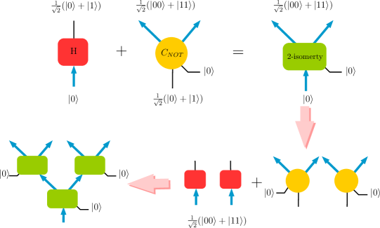
Figure 2: The computation process of the MERA circuit with the Bell gates.

References

- (1) J. D. Bekenstein, “Black holes and entropy,” Phys. Rev. D 7, 2333 (1973).
- (2) S. W. Hawking, “Black hole explosions,” Nature 248, 30 (1974).
- (3) G. ’t Hooft, “Dimensional reduction in quantum gravity,” Conf. Proc. C 930308, 284 (1993) [gr-qc/9310026].
- (4) L. Susskind, “The World as a hologram,” J. Math. Phys. 36, 6377 (1995)
- (5) J. M. Maldacena, “The Large N limit of superconformal field theories and supergravity,” Int. J. Theor. Phys. 38, 1113 (1999) [Adv. Theor. Math. Phys. 2, 231 (1998)]
- (6) E. Witten, “Anti-de Sitter space and holography,” Int. J. Theor. Phys. 2, 253 (1998)
- (7) S. Ryu and T. Takayanagi, “Holographic derivation of entanglement entropy from AdS/CFT,” Phys. Rev. Lett. 96, 181602 (2006)
- (8) M. Van Raamsdonk, “Building up spacetime with quantum entanglement,” Gen. Rel. Grav. 42, 2323 (2010) [Int. J. Mod. Phys. D 19, 2429 (2010)]
- (9) B. Swingle, “Entanglement Renormalization and Holography,” Phys. Rev. D 86, 065007 (2012)
- (10) G. Vidal, “Class of Quantum Many-Body States That Can Be Efficiently Simulated,” Phys. Rev. Lett. 101, 110501 (2008).
- (11) C. Beny, “Causal structure of the entanglement renormalization ansatz,” New J. Phys. 15, 023020 (2013)
- (12) B. Czech, L. Lamprou, S. McCandlish and J. Sully, “Integral Geometry and Holography,” JHEP 1510, 175 (2015)
- (13) B. Czech, L. Lamprou, S. McCandlish and J. Sully, “Tensor Networks from Kinematic Space,” JHEP 1607, 100 (2016)
- (14) C. T. Asplund, N. Callebaut and C. Zukowski, “Equivalence of Emergent de Sitter Spaces from Conformal Field Theory,” JHEP 1609, 154 (2016)
- (15) B. Czech, L. Lamprou, S. McCandlish, B. Mosk and J. Sully, “A Stereoscopic Look into the Bulk,” JHEP 1607, 129 (2016)
- (16) J. de Boer, M. P. Heller, R. C. Myers and Y. Neiman, “Holographic de Sitter Geometry from Entanglement in Conformal Field Theory,” Phys. Rev. Lett. 116, no. 6, 061602 (2016)
- (17) A. R. Brown, D. A. Roberts, L. Susskind, B. Swingle and Y. Zhao, “Holographic Complexity Equals Bulk Action?,” Phys. Rev. Lett. 116, no. 19, 191301 (2016)
- (18) A. R. Brown, D. A. Roberts, L. Susskind, B. Swingle and Y. Zhao, “Complexity, action, and black holes,” Phys. Rev. D 93, no. 8, 086006 (2016)
- (19) S. Chapman, H. Marrochio and R. C. Myers, “Complexity of Formation in Holography,” JHEP 1701, 062 (2017)
- (20) D. Carmi, R. C. Myers and P. Rath, “Comments on Holographic Complexity,” JHEP 1703, 118 (2017)
- (21) P. Caputa, N. Kundu, M. Miyaji, T. Takayanagi and K. Watanabe, “Anti-de Sitter Space from Optimization of Path Integrals in Conformal Field Theories,” Phys. Rev. Lett. 119, no. 7, 071602 (2017)
- (22) P. Caputa, N. Kundu, M. Miyaji, T. Takayanagi and K. Watanabe, “Liouville Action as Path-Integral Complexity: From Continuous Tensor Networks to AdS/CFT,” JHEP 1711, 097 (2017)
- (23) B. Czech, “Einstein Equations from Varying Complexity,” Phys. Rev. Lett. 120, no. 3, 031601 (2018)
- (24) A. Bhattacharyya, P. Caputa, S. R. Das, N. Kundu, M. Miyaji, T. Takayanagi, “Path-Integral Complexity for Perturbed CFTs,” [arXiv:1804.01999 [hep-th]].
- (25) N. Bao, C. J. Cao, S. M. Carroll and A. Chatwin-Davies, “De Sitter Space as a Tensor Network: Cosmic No-Hair, Complementarity, and Complexity,” Phys. Rev. D 96, no. 12, 123536 (2017)
- (26) B. Riemann, “Uber die hypothesen, wleche der geomterie zu grunde ligen,” in The collected works of B.Riemann, pp746-789, Dover NY (1953)
- (27) L. Bombelli, J. Lee, D. Meyer and R. D. Sorkin, “Space-Time as a Causal Set,” Phys. Rev. Lett. 59, 521 (1987).
- (28) R. Sinai Kunkolienkar and K. Banerjee, “Towards a dS/MERA correspondence,” Int. J. Mod. Phys. D 26, no. 13, 1750143 (2017)
- (29) L. P. Chimento, F. Pennini, A. Plastino, “Einstein’s gravitational action and Fisher’s information measure,” Phys. Lett. A 293 133 (2002)
- (30) B. R. Frieden, “Physics from Fisher Information,” Cambridge University Press, Cambridge, 1998.
- (31) C. Beck, F. Schgl, “Thermodynamics of Chaotic Systems,” Cambridge University Press, Cambridge, 1993.
- (32) M. Nozaki, T. Numasawa and T. Takayanagi, “Holographic Local Quenches and Entanglement Density,” JHEP 1305, 080 (2013)
- (33) L. Susskind, “Entanglement is not enough,” Fortsch. Phys. 64 (2016) 49-71
- (34) N. Bao, C. Cao, S. M. Carroll, L. McAllister, “Quantum Circuit Cosmology: The Expansion of the Universe Since the First Qubit,” [arXiv:1702.06959 [hep-th]].
- (35) J. D. Brown and M. Henneaux, “Central Charges in the Canonical Realization of Asymptotic Symmetries: An Example from Three-Dimensional Gravity,” Commun. Math. Phys. 104, 207 (1986).
- (36) S. Lloyd, “Ultimate physical limits to computation,” Nature 406 (Aug., 2000) ,
- (37) W. Cottrell and M. Montero, “Complexity is simple!,” JHEP 1802, 039 (2018)
- (38) M. Alishahiha, A. Faraji Astaneh, A. Naseh and M. H. Vahidinia, “On complexity for F(R) and critical gravity,” JHEP 1705, 009 (2017) [arXiv:1702.06796 [hep-th]].
- (39) S. Capozziello, “Curvature quintessence,” Int. J. Mod. Phys. D 11, 483 (2002)
- (40) A. Z. Grinshpan, “Weighted inequalities and negative binomials,” Advances in Applied Mathematics, 45 (4): 564šC606 (2010)
- (41) S. Chapman, M. P. Heller, H. Marrochio and F. Pastawski, “Toward a Definition of Complexity for Quantum Field Theory States,” Phys. Rev. Lett. 120, no. 12, 121602 (2018)
- (42) M. Nozaki, S. Ryu and T. Takayanagi, “Holographic Geometry of Entanglement Renormalization in Quantum Field Theories,” JHEP 1210, 193 (2012) [arXiv:1208.3469 [hep-th]].
- (43) J. M. Aldaz, S. Barza, M. Fujii, M. S. Moslehian, “Advances in Operator Cauchy¡ªSchwarz inequalities and their reverses,” Annals of Functional Analysis, 6 (3): 275-295 (2015).
- (44) E. G. Rieffel, W. H. Polak, “Quantum Computing: A Gentle Introduction” MIT Press.
- (45) C. Monroe, D. M. Meekhof, B. E. King, W. M. Itano and D. J. Wineland, “Demonstration of a Fundamental Quantum Logic Gate,” Phys. Rev. Lett. 75, 4714 (1995).