Composing Entropic Policies using Divergence Correction

Jonathan J Hunt    Andre Barreto    Timothy P Lillicrap    Nicolas Heess
Abstract

Composing previously mastered skills to solve novel tasks promises dramatic improvements in the data efficiency of reinforcement learning. Here, we analyze two recent works composing behaviors represented in the form of action-value functions and show that they perform poorly in some situations. As part of this analysis, we extend an important generalization of policy improvement to the maximum entropy framework and introduce an algorithm for the practical implementation of successor features in continuous action spaces. Then we propose a novel approach which addresses the failure cases of prior work and, in principle, recovers the optimal policy during transfer. This method works by explicitly learning the (discounted, future) divergence between base policies. We study this approach in the tabular case and on non-trivial continuous control problems with compositional structure and show that it outperforms or matches existing methods across all tasks considered.

Machine Learning, ICML

1 Introduction

Reinforcement learning (RL) algorithms coupled with powerful function approximators have recently achieved a series of successes (Mnih et al., 2015; Silver et al., 2016; Lillicrap et al., 2015; Kalashnikov et al., 2018). Unfortunately, all of these approaches still require a large number of interactions with the environment. One reason for this is that the algorithms are typically applied “from scratch,” rather than leveraging experience from prior tasks. This reduces their applicability in domains where generating experience is expensive, or learning from scratch is challenging.

In humans, the development of complex motor skills, such as bipedal locomotion or high-speed manipulation, also requires large amounts of experience and practice (Adolph et al., 2012; Haith & Krakauer, 2013) However, once such skills have been acquired humans rapidly put them to work in new contexts and to solve new tasks, suggesting transfer learning as an important mechanism for data efficiency.

Motivated by this observation, we are interested in RL methods for transfer that are suitable for high-dimensional motor control. We focus on model-free approaches which are evident in human motor control (Haith & Krakauer, 2013) and underlie the recent successes of Deep RL cited above.

Transfer may be especially valuable in domains where a small set of skills can be composed, in different combinations, to solve a variety of tasks. Different notions of compositionality have been considered in the RL and robotics literature. For instance, ‘options’ tend to be associated with discrete units of behavior that can be sequenced, thus emphasizing composition in time (Precup et al., 1998). In this paper we are concerned with a rather distinct notion of compositionality, namely how to combine and blend potentially concurrent behaviors. This form of composition is particularly relevant in high-dimensional continuous action spaces, where it is possible to achieve more than one task simultaneously (e.g. walking somewhere while juggling).

One approach to this challenge is via the composition of task rewards. Specifically, we are interested in the following question: If we have previously solved a set of tasks with similar transition dynamics but different reward functions, how can we leverage this knowledge to solve new tasks which can be expressed as a convex combination of those reward functions?

This question has recently been studied in two independent lines of work: by Barreto et al. (2017, 2018) in the context of successor feature (SF) representations used for Generalized Policy Improvement (GPI) with deterministic policies, and by Haarnoja et al. (2018a); van Niekerk et al. (2018) in the context of maximum entropy (max-ent) policies. These approaches operate in distinct frameworks but both achieve skill composition by combining the Q𝑄Q-functions associated with previously learned skills.

In this paper, we clarify the relationship between the two approaches and show that both perform well in some situations but that they fail in complementary ways. We introduce a novel method of behavior composition that can consistently achieve good performance.

Our contributions are as follows:

  1. 1.

    We introduce succcessor features (SF) in the context of the maximum entropy framework and extend the GPI theorem to the max-ent objective (max-ent GPI).

  2. 2.

    We provide an analysis of when GPI, and compositional “optimism” (CO) (Haarnoja et al., 2018a) perform poorly. We highlight these failure cases with tabular discrete action tasks and challenging continuous control tasks.

  3. 3.

    We propose a correction term – which we call Divergence Correction (DC)– based on the Rényi divergence between policies which allows us, in principle, to recover the optimal policy for transfer for any convex combination of rewards.

  4. 4.

    We demonstrate a practical algorithm, which relies of adaptive importance sampling, for zero-shot transfer with DC or max-ent GPI in continuous action spaces. We compare the approaches introduced here, max-ent GPI and DC, with compositional optimism (Haarnoja et al., 2018a) and Conditional Q𝑄Q functions (Schaul et al., 2015) in a variety of non-trivial continuous action transfer tasks.

2 Background

2.1 Multi-task RL

We consider Markov Decision Processes defined by the tuple \mathcal{M} containing: a state space 𝒮𝒮\mathcal{S}, action space 𝒜𝒜\mathcal{A}, start state distribution p(s1)𝑝subscript𝑠1p(s_{1}), transition function p(st+1|st,at)𝑝conditionalsubscript𝑠𝑡1subscript𝑠𝑡subscript𝑎𝑡p(s_{t+1}|s_{t},a_{t}), discount γ[0,1)𝛾01\gamma\in[0,1) and reward function r(st,at,st+1)𝑟subscript𝑠𝑡subscript𝑎𝑡subscript𝑠𝑡1r(s_{t},a_{t},s_{t+1}). We aim to find an optimal policy π(a|s):𝒮𝒫(𝒜):𝜋conditional𝑎𝑠𝒮𝒫𝒜\pi(a|s):\mathcal{S}\rightarrow\mathcal{P}(\mathcal{A}), which is one that maximises the discounted expected return from any state J(π)=𝔼π,[τ=tγτtrτ]𝐽𝜋subscript𝔼𝜋delimited-[]superscriptsubscript𝜏𝑡superscript𝛾𝜏𝑡subscript𝑟𝜏J(\pi)=\mathbb{E}_{\pi,\mathcal{M}}\left[\sum_{\tau=t}^{\infty}\gamma^{\tau-t}r_{\tau}\right] where the expected return is dependent on the policy π𝜋\pi and the MDP \mathcal{M}.

We formalize transfer as in Barreto et al. (2017); Haarnoja et al. (2018a), as the desire to perform well across all tasks in a set 𝒯superscript𝒯\mathcal{M}\in\mathcal{T}^{\prime} (without direct experience on these tasks) after having learned policies for tasks 𝒯𝒯\mathcal{M}\in\mathcal{T}. We assume that 𝒯𝒯\mathcal{T} and 𝒯superscript𝒯\mathcal{T}^{\prime} are related in two ways: all tasks share the same state transition function, and tasks in 𝒯superscript𝒯\mathcal{T}^{\prime} can be expressed as convex combinations of rewards associated with tasks in set 𝒯𝒯\mathcal{T}. We write the reward functions for tasks in 𝒯𝒯\mathcal{T} as the vector ϕ=(r1,r2,)bold-italic-ϕsubscript𝑟1subscript𝑟2{\bm{\phi}}=(r_{1},r_{2},\dots), so tasks in 𝒯superscript𝒯\mathcal{T}^{\prime} can be expressed as r𝐰=ϕ𝐰subscript𝑟𝐰bold-italic-ϕ𝐰r_{\mathbf{w}}={\bm{\phi}}\cdot\mathbf{w}. Our theoretical results assume that we have learned optimal policies for all tasks in 𝒯𝒯\mathcal{T}.

For clarity, we focus on the combination of only two policies, that is 𝐰𝐰\mathbf{w} has only 2 non-zero entries and so we can write rb=bri+(1b)rjsubscript𝑟𝑏𝑏subscript𝑟𝑖1𝑏subscript𝑟𝑗r_{b}=br_{i}+(1-b)r_{j} (b[0,1]𝑏01b\in[0,1]). As we discuss later, the approaches we consider can be extended to more than two tasks. We refer to a transfer method as optimal, if it results in an optimal policy for the transfer task in 𝒯superscript𝒯\mathcal{T}^{\prime}, using only experience on tasks 𝒯𝒯\mathcal{T}. As in most prior work in Deep RL, theoretical guarantees of optimality can only be approximately achieved in practise.

2.2 Successor Features

Successor Features (SF) (Dayan, 1993) and Generalised Policy Improvement (GPI) (Barreto et al., 2017, 2018) provide a principled solution to transfer in the setting defined above. SF make the additional assumption that the reward feature ϕbold-italic-ϕ{\bm{\phi}} is fully observable, that is, the agent always has access to the rewards of all tasks in 𝒯𝒯\mathcal{T} but not 𝒯superscript𝒯\mathcal{T}^{\prime} during training.

The key insight of SF is that linearity of the reward r𝐰subscript𝑟𝐰r_{\mathbf{w}} with respect to the features ϕbold-italic-ϕ{\bm{\phi}} implies the following decomposition of the action value of policy π𝜋\pi on task r𝐰subscript𝑟𝐰r_{\mathbf{w}}:

Q𝐰π(st,at)subscriptsuperscript𝑄𝜋𝐰subscript𝑠𝑡subscript𝑎𝑡\displaystyle\textstyle Q^{\pi}_{\mathbf{w}}(s_{t},a_{t}) =𝔼π[τ=tγτtϕτ𝐰|at]absentsubscript𝔼𝜋delimited-[]conditionalsuperscriptsubscript𝜏𝑡superscript𝛾𝜏𝑡subscriptbold-italic-ϕ𝜏𝐰subscript𝑎𝑡\displaystyle=\mathbb{E}_{\pi}\left[\sum_{\tau=t}^{\infty}\gamma^{\tau-t}{\bm{\phi}}_{\tau}\cdot\mathbf{w}|a_{t}\right]
=𝔼π[i=tγτtϕτ|at]𝐰𝝍π(st,at)𝐰absentsubscript𝔼𝜋delimited-[]conditionalsuperscriptsubscript𝑖𝑡superscript𝛾𝜏𝑡subscriptbold-italic-ϕ𝜏subscript𝑎𝑡𝐰superscript𝝍𝜋subscript𝑠𝑡subscript𝑎𝑡𝐰\displaystyle=\mathbb{E}_{\pi}\left[\sum_{i=t}^{\infty}\gamma^{\tau-t}{\bm{\phi}}_{\tau}|a_{t}\right]\cdot\mathbf{w}\equiv{\bm{\psi}}^{\pi}(s_{t},a_{t})\cdot\mathbf{w}

where 𝝍πsuperscript𝝍𝜋{\bm{\psi}}^{\pi} is the expected discounted sum of features ϕbold-italic-ϕ{\bm{\phi}} induced by policy π𝜋\pi. The SF decomposition allows us to compute the value of an existing policy π𝜋\pi on a new task r𝐰subscript𝑟𝐰r_{\mathbf{w}}.

GPI provides a principled way to use this value information to compose n𝑛n existing polices π1,π2,,πnsubscript𝜋1subscript𝜋2subscript𝜋𝑛\pi_{1},\pi_{2},...,\pi_{n} indexed by i𝑖i to solve task r𝐰subscript𝑟𝐰r_{\mathbf{w}}. Namely, we act according to the deterministic GPI policy π𝐰GPI(st)argmaxatQ𝐰GPI(st,at)subscriptsuperscript𝜋𝐺𝑃𝐼𝐰subscript𝑠𝑡subscriptargmaxsubscript𝑎𝑡subscriptsuperscript𝑄𝐺𝑃𝐼𝐰subscript𝑠𝑡subscript𝑎𝑡\pi^{GPI}_{\mathbf{w}}(s_{t})\equiv\operatorname*{arg\,max}_{a_{t}}Q^{GPI}_{\mathbf{w}}(s_{t},a_{t}) where

Q𝐰GPI(st,at)maxiQ𝐰πi(st,at)=maxi𝝍πi(s,a)𝐰subscriptsuperscript𝑄𝐺𝑃𝐼𝐰subscript𝑠𝑡subscript𝑎𝑡subscript𝑖subscriptsuperscript𝑄subscript𝜋𝑖𝐰subscript𝑠𝑡subscript𝑎𝑡subscript𝑖superscript𝝍subscript𝜋𝑖𝑠𝑎𝐰\displaystyle\textstyle Q^{GPI}_{\mathbf{w}}(s_{t},a_{t})\equiv\max_{i}Q^{\pi_{i}}_{\mathbf{w}}(s_{t},a_{t})=\max_{i}{\bm{\psi}}^{\pi_{i}}(s,a)\cdot\mathbf{w}

The GPI theorem guarantees the GPI policy has a return at least as good as any component policy, that is, V𝐰πGPI(s)maxiV𝐰πi(s)s𝒮subscriptsuperscript𝑉superscript𝜋𝐺𝑃𝐼𝐰𝑠subscript𝑖subscriptsuperscript𝑉subscript𝜋𝑖𝐰𝑠for-all𝑠𝒮V^{\pi^{GPI}}_{\mathbf{w}}(s)\geq\max_{i}V^{\pi_{i}}_{\mathbf{w}}(s)\>\forall s\in\mathcal{S}.

Note that SF and GPI are separate concepts, the GPI theorem does not require the use of SFs. SFs provide an efficient mechanism for computing the value of existing policies on a new task, and GPI provides a principled way to make use of this information to compose the existing policies.

2.3 Maximum Entropy RL

The maximum entropy (max-ent) RL objective augments the reward to favor entropic solutions

J(π)=𝔼π,[τ=tγτt(rτ+αH[π(|sτ))]]\displaystyle\textstyle J(\pi)=\mathbb{E}_{\pi,\mathcal{M}}\left[\sum_{\tau=t}^{\infty}\gamma^{\tau-t}(r_{\tau}+\alpha H[\pi(\cdot|s_{\tau}))]\right] (1)

where α𝛼\alpha is a parameter that determines the relative importance of the entropy term.

This objective has been considered in a number of works including (Kappen, 2005; Todorov, 2009; Haarnoja et al., 2017, 2018a; Ziebart et al., 2008; Fox et al., 2016).

We define the action-value Qπsuperscript𝑄𝜋Q^{\pi} associated with eq. 1 as

Qπ(st,at)rt+𝔼π[τ=t+1γτt(rτ+αH[π(|sτ)])]\displaystyle\textstyle Q^{\pi}(s_{t},a_{t})\equiv r_{t}+\mathbb{E}_{\pi}\left[\sum_{\tau={t+1}}^{\infty}\gamma^{\tau-t}(r_{\tau}+\alpha H[\pi(\cdot|s_{\tau})])\right] (2)

(notice Qπ(st,at)superscript𝑄𝜋subscript𝑠𝑡subscript𝑎𝑡Q^{\pi}(s_{t},a_{t}) does not include the entropy term for the state stsubscript𝑠𝑡s_{t}). Soft Q iteration where the policy π(at|st)exp(1αQ(st,at))proportional-to𝜋conditionalsubscript𝑎𝑡subscript𝑠𝑡1𝛼𝑄subscript𝑠𝑡subscript𝑎𝑡\pi(a_{t}|s_{t})\propto\exp(\frac{1}{\alpha}Q(s_{t},a_{t})) is implicitly defined by Q𝑄Q converges to the optimal policy with standard assumptions (Haarnoja et al., 2017).

Q(st,at)𝑄subscript𝑠𝑡subscript𝑎𝑡\displaystyle\textstyle Q(s_{t},a_{t}) r(st,at,st+1)+γ𝔼p(st+1|st,at)[V(st+1)]absent𝑟subscript𝑠𝑡subscript𝑎𝑡subscript𝑠𝑡1𝛾subscript𝔼𝑝conditionalsubscript𝑠𝑡1subscript𝑠𝑡subscript𝑎𝑡delimited-[]𝑉subscript𝑠𝑡1\displaystyle\leftarrow r(s_{t},a_{t},s_{t+1})+\gamma\mathbb{E}_{p(s_{t+1}|s_{t},a_{t})}\left[V(s_{t+1})\right]
V(st)𝑉subscript𝑠𝑡\displaystyle V(s_{t}) 𝔼π[Q(st,at)]+αH[π(|st)]\displaystyle\leftarrow\mathbb{E}_{{\pi}}\left[Q(s_{t},a_{t})\right]+\alpha H[\pi(\cdot|s_{t})]
=αlog𝒜exp(1αQ(st,at))𝑑aαlogZ(st)absent𝛼subscript𝒜1𝛼𝑄subscript𝑠𝑡subscript𝑎𝑡differential-d𝑎𝛼𝑍subscript𝑠𝑡\displaystyle=\alpha\log\int_{\mathcal{A}}\exp(\frac{1}{\alpha}Q(s_{t},a_{t}))da\equiv\alpha\log Z(s_{t})

2.4 Compositional Optimisim (CO)

Haarnoja et al. (2018a) introduced a simple approach to policy composition in the max-ent framework by approximating the optimal action-value for the transfer task rb=bri+(1b)rjsubscript𝑟𝑏𝑏subscript𝑟𝑖1𝑏subscript𝑟𝑗r_{b}=br_{i}+(1-b)r_{j} from the optimal action-values of the component tasks Qisuperscript𝑄𝑖Q^{i} and Qjsuperscript𝑄𝑗Q^{j}

QbCO(s,a)bQi(s,a)+(1b)Qj(s,a).superscriptsubscript𝑄𝑏𝐶𝑂𝑠𝑎𝑏superscript𝑄𝑖𝑠𝑎1𝑏superscript𝑄𝑗𝑠𝑎\displaystyle\textstyle Q_{b}^{CO}(s,a)\equiv bQ^{i}(s,a)+(1-b)Q^{j}(s,a). (3)

When using Boltzmann policies defined by Q𝑄Q, the resulting policy, πbCO(a|s)exp(1αQbCO(s,a))proportional-tosuperscriptsubscript𝜋𝑏𝐶𝑂conditional𝑎𝑠1𝛼superscriptsubscript𝑄𝑏𝐶𝑂𝑠𝑎\pi_{b}^{CO}(a|s)\propto\exp(\frac{1}{\alpha}Q_{b}^{CO}(s,a)), is the product distribution of the two component policies. We refer to πbCOsubscriptsuperscript𝜋𝐶𝑂𝑏\pi^{CO}_{b} as the compositionally “optimistic” (CO) policy, as it acts according to an over-estimate of the action value (QbCO(s,a)Qb(s,a)superscriptsubscript𝑄𝑏𝐶𝑂𝑠𝑎superscriptsubscript𝑄𝑏𝑠𝑎Q_{b}^{CO}(s,a)\geq Q_{b}^{*}(s,a)) by assuming the optimal returns of Qisuperscript𝑄𝑖Q^{i} and Qjsuperscript𝑄𝑗Q^{j} will be, simultaneously, achievable.

3 Composing Policies in Max-Ent Reinforcement Learning

In this section we present two novel approaches for transfer in the max-ent framework. In section 4 we then outline a practical algorithm using these results.

3.1 Max-Ent Successor Features and Generalized Policy Improvement

We introduce max-ent SF, which provide a mechanism for computing the value of a maximum entropy policy under any convex combination of rewards. We then show that the GPI theorem (Barreto et al., 2017) holds for maximum entropy policies.

We define the action-dependent SF to include the entropy of the policy, excluding the current state, analogous to the max-entropy definition of Qπsuperscript𝑄𝜋Q^{\pi} in (2):

𝝍π(st,at)superscript𝝍𝜋subscript𝑠𝑡subscript𝑎𝑡\displaystyle\textstyle{\bm{\psi}}^{\pi}(s_{t},a_{t}) ϕt+𝔼π[τ=i+1γτt(ϕτ+α𝟏H[π(|s)])]\displaystyle\equiv{\bm{\phi}}_{t}+\mathbb{E}_{\pi}\left[\sum_{\tau={i+1}}^{\infty}\gamma^{\tau-t}({\bm{\phi}}_{\tau}+\alpha\bm{1}\cdot H[\pi(\cdot|s)])\right]
=ϕt+γ𝔼p(st+1|st,at)[𝚼(st+1)]absentsubscriptitalic-ϕ𝑡𝛾subscript𝔼𝑝conditionalsubscript𝑠𝑡1subscript𝑠𝑡subscript𝑎𝑡delimited-[]𝚼subscript𝑠𝑡1\displaystyle=\phi_{t}+\gamma\mathbb{E}_{p(s_{t+1}|s_{t},a_{t})}\left[{\bm{\Upsilon}}(s_{t+1})\right]

where 𝟏1\bm{1} is a vector of ones of the same dimensionality as ϕitalic-ϕ\phi and we define the state-dependent successor features as the expected 𝝍πsuperscript𝝍𝜋{\bm{\psi}}^{\pi} in analogy with Vπ(s)superscript𝑉𝜋𝑠V^{\pi}(s):

𝚼π(s)𝔼aπ(|s)[𝝍π(s,a)]+α𝟏H[π(|s)].\displaystyle\textstyle{\bm{\Upsilon}}^{\pi}(s)\equiv\mathbb{E}_{a\sim\pi(\cdot|s)}\left[{\bm{\psi}}^{\pi}(s,a)\right]+\alpha\bm{1}\cdot H[\pi(\cdot|s)]. (4)

The max-entropy action-value of π𝜋\pi for any convex combination of rewards 𝐰𝐰\mathbf{w} is then given by Q𝐰π(s,a)=𝝍π(s,a)𝐰subscriptsuperscript𝑄𝜋𝐰𝑠𝑎superscript𝝍𝜋𝑠𝑎𝐰Q^{\pi}_{\mathbf{w}}(s,a)={\bm{\psi}}^{\pi}(s,a)\cdot\mathbf{w}. Max-ent SF allow us to estimate the action-value of previous policies on a new task. We show that, as in the deterministic case, there is a principled way to combine multiple policies using their action-values on task 𝐰𝐰\mathbf{w}.

Theorem 3.1 (Max-Ent Generalized Policy Improvement)

Let π1,π2,,πnsubscript𝜋1subscript𝜋2subscript𝜋𝑛\pi_{1},\pi_{2},...,\pi_{n} be n𝑛n policies with α𝛼\alpha-max-ent action-value functions Q1,Q2,,Qnsuperscript𝑄1superscript𝑄2superscript𝑄𝑛Q^{1},Q^{2},...,Q^{n} and value functions V1,V2,,Vnsuperscript𝑉1superscript𝑉2superscript𝑉𝑛V^{1},V^{2},...,V^{n}. Define

π(a|s)exp(1αmaxiQi(s,a)).proportional-to𝜋conditional𝑎𝑠1𝛼subscript𝑖superscript𝑄𝑖𝑠𝑎\displaystyle\textstyle\pi(a|s)\propto\exp\left(\frac{1}{\alpha}\max_{i}Q^{i}(s,a)\right).

Then,

Qπ(s,a)superscript𝑄𝜋𝑠𝑎\displaystyle\textstyle Q^{\pi}(s,a) maxiQi(s,a) for all s𝒮a𝒜,absentsubscript𝑖superscript𝑄𝑖𝑠𝑎 for all s𝒮a𝒜,\displaystyle\geq\max_{i}Q^{i}(s,a)\text{ for all $s\in\mathcal{S}$, $a\in\mathcal{A}$,} (5)
Vπ(s)superscript𝑉𝜋𝑠\displaystyle V^{\pi}(s) maxiVi(s) for all s𝒮,absentsubscript𝑖superscript𝑉𝑖𝑠 for all s𝒮,\displaystyle\geq\max_{i}V^{i}(s)\text{ for all $s\in\mathcal{S}$, } (6)

where Qπ(s,a)superscript𝑄𝜋𝑠𝑎Q^{\pi}(s,a) and Vπ(s)superscript𝑉𝜋𝑠V^{\pi}(s) are the α𝛼\alpha-max-ent action-value and value function respectively of π𝜋\pi.

Proof: See appendix A.1.

In our setup, we learn 𝝍πi(s,a)superscript𝝍subscript𝜋𝑖𝑠𝑎{\bm{\psi}}^{\pi_{i}}(s,a), the SFs of policies πisubscript𝜋𝑖\pi_{i} for each task in 𝒯𝒯\mathcal{T}, we define the max-ent GPI policy for task 𝐰𝒯𝐰superscript𝒯\mathbf{w}\in\mathcal{T^{\prime}} as π𝐰GPI(a|s)exp(1αmaxiQ𝐰πi(s,a))=exp(1αmaxi𝝍πi(s,a)𝐰).proportional-tosuperscriptsubscript𝜋𝐰𝐺𝑃𝐼conditional𝑎𝑠1𝛼subscript𝑖subscriptsuperscript𝑄subscript𝜋𝑖𝐰𝑠𝑎1𝛼subscript𝑖superscript𝝍subscript𝜋𝑖𝑠𝑎𝐰\pi_{\mathbf{w}}^{GPI}(a|s)\propto\exp(\frac{1}{\alpha}\max_{i}Q^{\pi_{i}}_{\mathbf{w}}(s,a))=\exp(\frac{1}{\alpha}\max_{i}{\bm{\psi}}^{\pi_{i}}(s,a)\cdot\mathbf{w}). In contrast to CO, GPI can be seen as acting “pessimistically” as it always acts according to a lower bound (equation 5) on the action-value.

3.2 Divergence Correction (DC)

Both max-ent GPI we presented above, and CO can, in different ways, fail to transfer well in some situations (fig.  1). Neither approach consistently acts optimally during transfer, even if all component terms are known exactly.

Here we show, at the cost of learning a function conditional on the task weightings b𝑏b, it is in principle possible to recover the optimal max-ent policy for the transfer tasks, without direct experience on those tasks, by correcting for the compositional optimism bias in QbCOsuperscriptsubscript𝑄𝑏𝐶𝑂Q_{b}^{CO}.

The correction term for CO uses a property noted, but not exploited in Haarnoja et al. (2018a). The bias in QCOsuperscript𝑄𝐶𝑂Q^{CO} is related to the the discounted sum of Rényi divergences of the two component policies. Intuitively, if the two policies induce trajectories with low divergence between the policies in each state, the CO assumption that both policies can achieve good returns simultaneously is approximately correct. When the divergences are large (i.e. the two policies do not agree on what action to take), the CO assumption is being overly optimistic.

Theorem 3.2 (DC Optimality)

Let πi,πjsubscript𝜋𝑖subscript𝜋𝑗\pi_{i},\pi_{j} be α𝛼\alpha max-ent optimal policies for tasks with rewards risubscript𝑟𝑖r_{i} and rjsubscript𝑟𝑗r_{j} with max-ent action-value functions Qi,Qjsuperscript𝑄𝑖superscript𝑄𝑗Q^{i},Q^{j}. Define Cb(st,at)subscriptsuperscript𝐶𝑏subscript𝑠𝑡subscript𝑎𝑡C^{\infty}_{b}(s_{t},a_{t}) as the fixed point of

Cb(k+1)(st,at)=αγ𝔼p(st+1|st,at)[log𝒜πi(at+1|st+1)bπj(at+1|st+1)(1b)exp(1αCb(k)(st+1,at+1))dat+1]subscriptsuperscript𝐶𝑘1𝑏subscript𝑠𝑡subscript𝑎𝑡𝛼𝛾subscript𝔼𝑝conditionalsubscript𝑠𝑡1subscript𝑠𝑡subscript𝑎𝑡delimited-[]subscript𝒜subscript𝜋𝑖superscript|subscript𝑎𝑡1subscript𝑠𝑡1𝑏subscript𝜋𝑗superscript|subscript𝑎𝑡1subscript𝑠𝑡11𝑏1𝛼subscriptsuperscript𝐶𝑘𝑏subscript𝑠𝑡1subscript𝑎𝑡1𝑑subscript𝑎𝑡1\begin{multlined}{C^{(k+1)}_{b}(s_{t},a_{t})=-\alpha\gamma\mathbb{E}_{p(s_{t+1}|s_{t},a_{t})}\Big{[}}\\ {\log\int_{\mathcal{A}}\pi_{i}(a_{t+1}|s_{t+1})^{b}\pi_{j}(a_{t+1}|s_{t+1})^{(1-b)}\exp\big{(}}\\ {-\frac{1}{\alpha}C^{(k)}_{b}(s_{t+1},a_{t+1})\big{)}da_{t+1}\Big{]}}\end{multlined}{C^{(k+1)}_{b}(s_{t},a_{t})=-\alpha\gamma\mathbb{E}_{p(s_{t+1}|s_{t},a_{t})}\Big{[}}\\ {\log\int_{\mathcal{A}}\pi_{i}(a_{t+1}|s_{t+1})^{b}\pi_{j}(a_{t+1}|s_{t+1})^{(1-b)}\exp\big{(}}\\ {-\frac{1}{\alpha}C^{(k)}_{b}(s_{t+1},a_{t+1})\big{)}da_{t+1}\Big{]}}

Given the conditions for Soft Q convergence, the max-ent optimal Qb(s,a)subscriptsuperscript𝑄𝑏𝑠𝑎Q^{*}_{b}(s,a) for rb=bri+(1b)rjsubscript𝑟𝑏𝑏subscript𝑟𝑖1𝑏subscript𝑟𝑗r_{b}=br_{i}+(1-b)r_{j} is

Qb(s,a)=bQi(s,a)+(1b)Qj(s,a)Cb(s,a)subscriptsuperscript𝑄𝑏𝑠𝑎𝑏superscript𝑄𝑖𝑠𝑎1𝑏superscript𝑄𝑗𝑠𝑎subscriptsuperscript𝐶𝑏𝑠𝑎\displaystyle Q^{*}_{b}(s,a)=bQ^{i}(s,a)+(1-b)Q^{j}(s,a)-C^{\infty}_{b}(s,a)
s𝒮,a𝒜,b[0,1]formulae-sequencefor-all𝑠𝒮formulae-sequence𝑎𝒜𝑏01\displaystyle\forall s\in\mathcal{S},a\in\mathcal{A},b\in[0,1]

Proof: See appendix A.2.

We call this Divergence Correction (DC) as the quantity Cbsubscriptsuperscript𝐶𝑏C^{\infty}_{b} is related to the Rényi divergence between policies (see appendix A.2 for details). Learning Cbsubscriptsuperscript𝐶𝑏C^{\infty}_{b} does not require any additional information (in principle) than that required to learn policies πisubscript𝜋𝑖\pi_{i} and πjsubscript𝜋𝑗\pi_{j}. Unlike with SF, it is not necessary to observe other task rewards while training the policies. On the other hand, SF/GPI can be used to combine any number of tasks with arbitrary weight vectors 𝐰𝐰\mathbf{w}, the difficulty of estimating Csuperscript𝐶C^{\infty} increases significantly if more than two tasks are combined (see supplementary theorem A1).

Supplementary Table 1 provides a comparison on the properties of the methods we consider here. We also compare with simply learning a conditional Q𝑄Q function Q(s,a|b)𝑄𝑠conditional𝑎𝑏Q(s,a|b) (CondQ) (e.g. Schaul et al., 2015; Andrychowicz et al., 2017). As with GPI, this requires observing the full set of task features ϕbold-italic-ϕ{\bm{\phi}}, in order to compute rbsubscript𝑟𝑏r_{b} for arbitrary b𝑏b.

We have introduced two new approaches to max-ent transfer composition and described their properties: max-ent SF/GPI and DC. Now we address the question of how to practically learn and sample with these approaches in continuous action spaces.

4 Adaptive Importance Sampling for Boltzman Policies Algorithm

Robotic systems with high-dimensional continuous action spaces are promising use cases for the ideas presented above, particularly as data efficiency is often a paramount concern. Such control problems may allow for multiple solutions, and often contain exploitable compositional structure.

Unfortunately, learning and sampling of general Boltzmann policies defined over continuous action spaces is challenging. One approach is to fit an expressible, tractable sampler, such as a stochastic neural network to approximate πisubscript𝜋𝑖\pi_{i} (e.g. Haarnoja et al., 2018a). This approach works well when learning a single policy. However, during transfer this may require learning a new sampler for each new transfer task. Here we want to zero-shot transfer by sampling from a newly synthesized action-value function online, which precludes fitting a sampler. To address this issue we introduce Adaptive Importance Sampling for Boltzmann Policies (AISBP), which provides a practical solution to this challenge.

We use parametric approximators (e.g. neural networks) and denote their parameters θ𝜃\theta, including the soft action-value for reward i𝑖i: QθQi(s,a)subscriptsuperscript𝑄𝑖subscript𝜃𝑄𝑠𝑎Q^{i}_{\theta_{Q}}(s,a); the associated soft value function VθVi(s)subscriptsuperscript𝑉𝑖subscript𝜃𝑉𝑠V^{i}_{\theta_{V}}(s) and a proposal distribution qθqi(a|s)subscriptsuperscript𝑞𝑖subscript𝜃𝑞conditional𝑎𝑠q^{i}_{\theta_{q}}(a|s), which is used for importance sampling the policy (we will sometimes drop the task index i𝑖i for notational simplicity, and write the losses for a single policy).

We use an off-policy algorithm, so that experience generated by training on policy πisubscript𝜋𝑖\pi_{i} can be used to improve policy πjsubscript𝜋𝑗\pi_{j}. This is important to ensure that QθQj(s,a)subscriptsuperscript𝑄𝑗subscript𝜃𝑄𝑠𝑎Q^{j}_{\theta_{Q}}(s,a) is a good approximation of the action-value function in states that are likely under πjsubscript𝜋𝑗\pi_{j} but unlikely under πisubscript𝜋𝑖\pi_{i} (suppl. F discusses issues of exploration and coverage of the state space under function approximation). Training experience across all tasks is stored in a replay buffer R𝑅R, and mini-batches of experience are sampled uniformly from the replay.

The proposal distribution is a mixture of M𝑀M truncated Normal distributions 𝒩Tsubscript𝒩𝑇\mathcal{N}_{T}, truncated to the square a[1,1)n𝑎superscript11𝑛a\in[-1,1)^{n} with diagonal covariances.

qθq(a|s)=1Mm=1M𝒩T(a;μθqm(s),σθqm(s),1,1)subscript𝑞subscript𝜃𝑞conditional𝑎𝑠1𝑀superscriptsubscript𝑚1𝑀subscript𝒩𝑇𝑎subscriptsuperscript𝜇𝑚subscript𝜃𝑞𝑠subscriptsuperscript𝜎𝑚subscript𝜃𝑞𝑠11\displaystyle\textstyle q_{\theta_{q}}(a|s)=\frac{1}{M}\sum_{m=1}^{M}\mathcal{N}_{T}(a;\mu^{m}_{\theta_{q}}(s),\sigma^{m}_{\theta_{q}}(s),-1,1) (7)

The proposal distribution is optimized by minimizing the forward KL divergence with the Boltzmann policy π(a|s)exp1αQθQ(s,a)proportional-to𝜋conditional𝑎𝑠1𝛼subscript𝑄subscript𝜃𝑄𝑠𝑎\pi(a|s)\propto\exp\frac{1}{\alpha}Q_{\theta_{Q}}(s,a). This KL is “zero avoiding” and over-estimates the support of π𝜋\pi (Murphy, 2012) which is desirable for a proposal distribution (Gu et al., 2015). The proposal loss is

(θq)subscript𝜃𝑞\displaystyle\textstyle\mathcal{L}(\theta_{q}) =𝔼R[𝔼aπ(|s)[logπ(a|st)logqθq(a|st)]]\displaystyle=\mathbb{E}_{R}\left[\mathbb{E}_{a\sim\pi(\cdot|s)}[\log\pi(a|s_{t})-\log q_{\theta_{q}}(a|s_{t})]\right] (8)

where the expectation is over the replay buffer state density.

The inner expectation in the proposal loss itself requires sampling from π𝜋\pi. We approximate this expectation by self-normalized importance sampling and use a target proposal distribution p(at|st)𝑝conditionalsubscript𝑎𝑡subscript𝑠𝑡p(a_{t}|s_{t}) which is a mixture distribution consisting of the proposals for all policies along with a uniform distribution. For batchsize B𝐵B and N𝑁N proposal action samples the estimator of the proposal loss is then

(θq)1Bk=1Bl=1Nwkllogqθq(akl|sk)wkl=exp1α(QθQ(sk,akl))p(akl|sk);wkl=wklm=1Nwkmformulae-sequencesubscript𝜃𝑞1𝐵superscriptsubscript𝑘1𝐵superscriptsubscript𝑙1𝑁subscript𝑤𝑘𝑙subscript𝑞subscript𝜃𝑞conditionalsubscript𝑎𝑘𝑙subscript𝑠𝑘subscriptsuperscript𝑤𝑘𝑙1𝛼subscript𝑄subscript𝜃𝑄subscript𝑠𝑘subscript𝑎𝑘𝑙𝑝conditionalsubscript𝑎𝑘𝑙subscript𝑠𝑘subscript𝑤𝑘𝑙subscriptsuperscript𝑤𝑘𝑙superscriptsubscript𝑚1𝑁subscriptsuperscript𝑤𝑘𝑚\begin{split}\textstyle\mathcal{L}(\theta_{q})&\approx-\frac{1}{B}\sum_{k=1}^{B}\sum_{l=1}^{N}w_{kl}\log q_{\theta_{q}}(a_{kl}|s_{k})\\ w^{\prime}_{kl}&=\frac{\exp\frac{1}{\alpha}(Q_{\theta_{Q}}(s_{k},a_{kl}))}{p(a_{kl}|s_{k})};\>\>w_{kl}=\frac{w^{\prime}_{kl}}{\sum_{m=1}^{N}w^{\prime}_{km}}\end{split}

By restricting the proposal distribution to mixtures of (truncated) Gaussians, we ensure the product of the proposal distributions is tractable. We make use of this product proposal during transfer (see supplementary C.3).

The policy is improved using Soft Q iteration (eq. 2). The value function loss is defined as the L2 error on the Soft Q estimate of value

(θV)=𝔼R[12(VθV(st)αlog𝒜exp(1αQθQ(st,a))da)2]subscript𝜃𝑉subscript𝔼𝑅delimited-[]12superscriptsubscript𝑉subscript𝜃𝑉subscript𝑠𝑡𝛼subscript𝒜1𝛼subscript𝑄subscript𝜃𝑄subscript𝑠𝑡𝑎𝑑𝑎2\begin{split}\textstyle\mathcal{L}(\theta_{V})=\>\mathbb{E}_{R}\Big{[}\frac{1}{2}\Big{(}&V_{\theta_{V}}(s_{t})-\\ &\alpha\log\int_{\mathcal{A}}\exp(\frac{1}{\alpha}Q_{\theta_{Q}}(s_{t},a))da\Big{)}^{2}\Big{]}\end{split} (9)

which is estimated using importance sampling to compute the integral.

(θV)12Bl=1B(VθV(sl)αlogZ)2Z=[1Nk=1Nexp(1αQθQ(sl,alk))qθq(alk|sl)]subscript𝜃𝑉12𝐵superscriptsubscript𝑙1𝐵superscriptsubscript𝑉subscript𝜃𝑉subscript𝑠𝑙𝛼𝑍2𝑍delimited-[]1𝑁superscriptsubscript𝑘1𝑁1𝛼subscript𝑄subscript𝜃𝑄subscript𝑠𝑙subscript𝑎𝑙𝑘subscript𝑞subscript𝜃𝑞conditionalsubscript𝑎𝑙𝑘subscript𝑠𝑙\begin{split}\textstyle\mathcal{L}(\theta_{V})\approx\frac{1}{2B}\sum_{l=1}^{B}\left(V_{\theta_{V}}(s_{l})-\alpha\log Z\right)^{2}\\ Z=\left[\frac{1}{N}\sum_{k=1}^{N}\frac{\exp(\frac{1}{\alpha}Q_{\theta_{Q}}(s_{l},a_{lk}))}{q_{\theta_{q}}(a_{lk}|s_{l})}\right]\end{split} (10)

This introduces bias due to the finite-sample approximation of the expectation inside the (concave) log\log. In practice we found this estimator sufficiently accurate, provided the proposal distribution was close to π𝜋\pi. We also use importance sampling to sample from π𝜋\pi while acting.

The action-value loss is the L2 norm with the Soft Q target:

(θQ)=𝔼R[12(\displaystyle\textstyle\mathcal{L}(\theta_{Q})=\>\mathbb{E}_{R}\Big{[}\frac{1}{2}( QθQ(st,at)limit-fromsubscript𝑄subscript𝜃𝑄subscript𝑠𝑡subscript𝑎𝑡\displaystyle Q_{\theta_{Q}}(s_{t},a_{t})-
(r(st,at,st+1)+γVθV(st+1)))2]\displaystyle(r(s_{t},a_{t},s_{t+1})+\gamma V_{\theta_{V}^{\prime}}(s_{t+1})))^{2}\Big{]} (11)

To improve stability we employ target networks for the value VθVsubscript𝑉subscript𝜃superscript𝑉V_{\theta_{V^{\prime}}} and proposal qθqsubscript𝑞superscriptsubscript𝜃𝑞q_{\theta_{q}^{\prime}} networks (Mnih et al., 2015; Lillicrap et al., 2015) We also parameterize Q𝑄Q as an advantage QθQ(s,a)=VθV(s)+AθA(s,a)subscript𝑄subscript𝜃𝑄𝑠𝑎subscript𝑉subscript𝜃𝑉𝑠subscript𝐴subscript𝜃𝐴𝑠𝑎Q_{\theta_{Q}}(s,a)=V_{\theta_{V}}(s)+A_{\theta_{A}}(s,a) (Baird, 1994; Wang et al., 2015; Harmon et al., 1995) which is more stable when the advantage is small compared with the value. The full algorithm is given in Algorithm 1 and more details are provided in appendix C.
Initialize proposal network parameters θqsubscript𝜃𝑞\theta_{q}
Initial value network parameters θVsubscript𝜃𝑉\theta_{V}
Initialize action-value network parameters θQsubscript𝜃𝑄\theta_{Q}
Initialize replay R𝑅R
while training do \triangleright in parallel on each actor
     Obtain parameters θ𝜃\theta from learner
     Sample task i𝒯similar-to𝑖𝒯i\sim\mathcal{T}
     Importance sample πi(a|s)exp1αQθQi(s,a)proportional-tosubscript𝜋𝑖conditional𝑎𝑠1𝛼subscriptsuperscript𝑄𝑖subscript𝜃𝑄𝑠𝑎\pi_{i}(a|s)\propto\exp\frac{1}{\alpha}Q^{i}_{\theta_{Q}}(s,a)
         Using proposal qθqisubscriptsuperscript𝑞𝑖subscript𝜃𝑞q^{i}_{\theta_{q}}
     Add experience to replay R𝑅R
end while
while training do \triangleright in parallel on the learner
     Sample SARS tuple from R𝑅R
     Improve (θq)subscript𝜃𝑞\mathcal{L}(\theta_{q}), (θV)subscript𝜃𝑉\mathcal{L}(\theta_{V}), (θQ)subscript𝜃𝑄\mathcal{L}(\theta_{Q})
     Improve additional losses for transfer
         (θ𝚼)subscript𝜃𝚼\mathcal{L}(\theta_{{\bm{\Upsilon}}}), (θ𝝍)subscript𝜃𝝍\mathcal{L}(\theta_{{\bm{\psi}}}), (θC)subscript𝜃𝐶\mathcal{L}(\theta_{C}), (θVb)subscript𝜃subscript𝑉𝑏\mathcal{L}(\theta_{V_{b}}) (θQb)subscript𝜃subscript𝑄𝑏\mathcal{L}(\theta_{Q_{b}}),
     if target update period then
         Update target network parameters
             θVθV,θqθqformulae-sequencesubscript𝜃superscript𝑉subscript𝜃𝑉subscript𝜃superscript𝑞subscript𝜃𝑞\theta_{V^{\prime}}\leftarrow\theta_{V},\theta_{q^{\prime}}\leftarrow\theta_{q}, θ𝚼θ𝚼subscript𝜃superscript𝚼subscript𝜃𝚼\theta_{{\bm{\Upsilon}}^{\prime}}\leftarrow\theta_{{\bm{\Upsilon}}}, θVbθVbsubscript𝜃superscriptsubscript𝑉𝑏subscript𝜃subscript𝑉𝑏\theta_{V_{b}^{\prime}}\leftarrow\theta_{V_{b}}
     end if
end while
Algorithm 1 AISBP training algorithm
Refer to caption
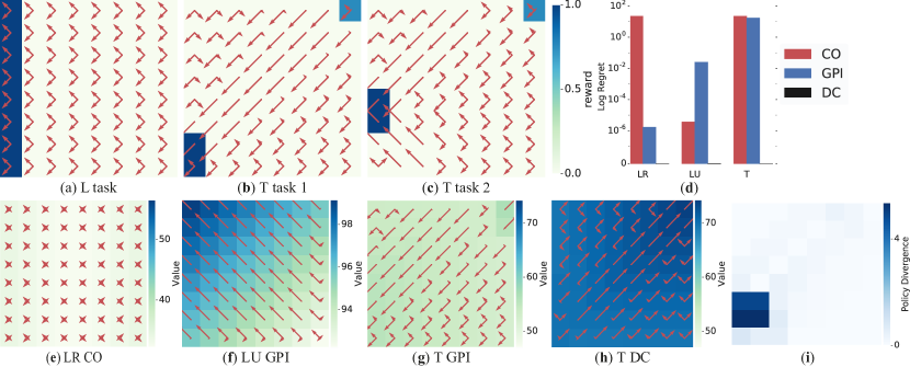
Figure 1: Policy composition in the tabular case. All tasks are in an infinite-horizon tabular 8x8 world. The action space is the 4 diagonal movements (actions at the boundary transition back to the same state) (a-c) shows the reward functions for the L(eft) task and the two T(ricky) tasks (color indicates reward, dark blue r=+1𝑟1r=+1, light blue r=0.75𝑟0.75r=0.75). The arrows indicate the action likelihoods for the max-ent optimal policy for each task. (d) The log regret on the compositional task rb=1/2ri+1/2rjsubscript𝑟𝑏12subscript𝑟𝑖12subscript𝑟𝑗r_{b}=1/2r_{i}+1/2r_{j} using the different methods for transfer. This is shown for three, qualitatively distinct compositional tasks: left-right (LR), left-up (LU) and the “tricky“ tasks (T). GPI performs well on LR, where the subtasks are incompatible, meaning the optimal policy on the transfer task is similar to one of the existing policies. In LR CO fails to commit to a particular direction (e shows the CO policy and value) and performs poorly. Conversely, on the LU task when the base policies are compatible, CO transfers well while the GPI policy (f) does not consistently take advantage of the compatibility of the two tasks to simultaneously achieve both base rewards (unlike the CO policy suppl. figure 5c). Neither GPI nor CO policies (g shows the GPI policy, but CO is similar) perform well when the optimal transfer policy is unlike either existing task policy. The two tricky task policies are compatible in many states but have a high-divergence in the bottom-left corner since the rewards are non-overlapping there (i shows the divergence in each state of the two tricky base policies), thus the optimal policy on the compositional transfer task is to move to the top right corner where there are overlapping rewards. By learning, and correcting for, this future divergence between policies, DC results in optimal policies for all task combinations including tricky (h). Additional details in suppl. figure 5.

4.1 Importance Sampled Max-Ent GPI

The same importance sampling approach can also be used to estimate max-ent SFs. Max-ent GPI requires us to learn the expected (maximum entropy) features 𝝍isubscript𝝍𝑖{\bm{\psi}}_{i} for each policy πisubscript𝜋𝑖\pi_{i}, in order to estimate its (entropic) value under a new convex combination task 𝐰𝐰\mathbf{w}. This requires that the experience tuples in the replay contain the full feature vector ϕbold-italic-ϕ{\bm{\phi}}, rather than just the reward for the policy which generated the experience risubscript𝑟𝑖r_{i}. Given this information 𝝍θ𝝍subscript𝝍subscript𝜃𝝍{\bm{\psi}}_{\theta_{\bm{\psi}}} and 𝚼θ𝚼subscript𝚼subscript𝜃𝚼{\bm{\Upsilon}}_{\theta_{\bm{\Upsilon}}} can be learned with analogous updates to V𝑉V and Q𝑄Q.

As with VθVsubscript𝑉subscript𝜃𝑉V_{\theta_{V}}, we use a target network for 𝚼θ𝚼subscript𝚼superscriptsubscript𝜃𝚼{\bm{\Upsilon}}_{\theta_{\bm{\Upsilon}}^{\prime}} and advantage parametrization. We found it more stable to using a larger target update period than for V𝑉V. Full details are of the losses and samplers are in appendix C.
Refer to caption
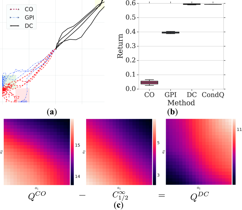
Figure 2: Tricky point mass. The continuous “tricky” task with a 2-D velocity controlled pointed mass. (a) Environment and example trajectories. The rewards are (r1=1,r2=0)formulae-sequencesubscript𝑟11subscript𝑟20(r_{1}=1,r_{2}=0), (0,1)01(0,1) and (0.75,0.75)0.750.75(0.75,0.75) for the green, red and yellow squares respectively. Lines show sampled trajectories (starting in the center) for the compositional task r1/2subscript𝑟12r_{1/2} with different transfer methods. Only DC and CondQ (not shown) navigate to the yellow reward area during transfer, which is the optimal reward. (b) Box plot of returns for each transfer method (5 seeds). DC and CondQ methods perform significantly better than GPI, and the CO policy performs poorly. (c) QCOsuperscript𝑄𝐶𝑂Q^{CO} at the center position for the transfer task. As both base policies prefer moving left and down, most of the energy (brighter color) is on these actions. However, the future divergence C1/2superscriptsubscript𝐶12C_{1/2}^{\infty} under these actions is high, which results in the QDCsuperscript𝑄𝐷𝐶Q^{DC} differing qualitatively from CO and favoring the upward trajectory. Additional details in supplementary figure 6.

4.2 Divergence Correction

Transfer using compositional optimism (equation 3, Haarnoja et al. (2018a)) only requires the max-ent action values of each task, so no additional training is required beyond the base policies. In section 3.2 we have shown that if we can learn the fixed point of Cb(s,a)subscriptsuperscript𝐶𝑏𝑠𝑎C^{\infty}_{b}(s,a) we can correct this compositional optimism bias and recover the optimal action-value Qb(s,a)subscriptsuperscript𝑄𝑏𝑠𝑎Q^{*}_{b}(s,a) for the transfer task rbsubscript𝑟𝑏r_{b}.

We exploit the recursive relationship in Cb(s,a)subscriptsuperscript𝐶𝑏𝑠𝑎C^{\infty}_{b}(s,a) to fit a neural net CθC(s,a,b)subscript𝐶subscript𝜃𝐶𝑠𝑎𝑏C_{\theta_{C}}(s,a,b) with a TD(0) estimator. This requires learning a conditional estimator for any value of b𝑏b, so as to support arbitrary task combinations. Fortunately, the same experience can be used to learn an estimator for all values of b𝑏b, by sampling b𝑏b during each TD update. We learn an estimator CθC(s,a,b)subscript𝐶subscript𝜃𝐶𝑠𝑎𝑏C_{\theta_{C}}(s,a,b) for each pair of policies πi,πjsubscript𝜋𝑖subscript𝜋𝑗\pi_{i},\pi_{j} with the loss

(θC)=𝔼sR,bU(0,1)[12(CθC(s,a,b)+αγ𝔼p(s|s,a)[log𝒜exp(blogπi(a|s)+(1b)πj(a|s)1αCθC(s,a,b))da])2]subscript𝜃𝐶subscript𝔼formulae-sequencesimilar-to𝑠𝑅similar-to𝑏𝑈01delimited-[]12superscriptsubscript𝐶subscript𝜃𝐶𝑠𝑎𝑏𝛼𝛾subscript𝔼𝑝conditionalsuperscript𝑠𝑠𝑎delimited-[]subscript𝒜𝑏subscript𝜋𝑖|superscript𝑎superscript𝑠1𝑏subscript𝜋𝑗|superscript𝑎superscript𝑠1𝛼subscript𝐶subscript𝜃superscript𝐶superscript𝑠superscript𝑎𝑏𝑑superscript𝑎2\begin{split}\textstyle\mathcal{L}(\theta_{C})=&\mathbb{E}_{s\sim R,b\sim U(0,1)}[\frac{1}{2}(C_{\theta_{C}}(s,a,b)+\\ &\alpha\gamma\mathbb{E}_{p(s^{\prime}|s,a)}[\log\int_{\mathcal{A}}\exp(b\log\pi_{i}(a^{\prime}|s^{\prime})+\\ &(1-b)\pi_{j}(a^{\prime}|s^{\prime})-\frac{1}{\alpha}C_{\theta_{C^{\prime}}}(s^{\prime},a^{\prime},b))da^{\prime}])^{2}]\end{split} (12)

As with other integrals of the action space, we approximate this loss using importance sampling to estimate the integral. As before, we use target networks and an advantage parametrization for CθC(s,a,b)subscript𝐶subscript𝜃𝐶𝑠𝑎𝑏C_{\theta_{C}}(s,a,b) Note that, unlike GPI and CondQ (next section), learning Cbsubscriptsuperscript𝐶𝑏C^{\infty}_{b} does not require observing ϕitalic-ϕ\phi while training.

We also considered a heuristic approach where we learned C𝐶C only for b=12𝑏12b=\frac{1}{2} (this is typically approximately the largest divergence). This avoids the complexity of a conditional estimator and then we we estimate Cbsuperscriptsubscript𝐶𝑏C_{b}^{\infty} during transfer as C^b(s,a)4b(1b)C1/2(s,a).similar-tosuperscriptsubscript^𝐶𝑏𝑠𝑎4𝑏1𝑏superscriptsubscript𝐶12𝑠𝑎\hat{C}_{b}^{\infty}(s,a)\sim 4b(1-b)C_{1/2}^{\infty}(s,a). This heuristic, we denote DC-Cheap, can be motivated by considering Gaussian policies (see appendix D) The max-ent GPI bound can be used to correct for over-estimates of the heuristic Cbsuperscriptsubscript𝐶𝑏C_{b}^{\infty}, QDCCheap+GPI(s,a)=max(QCO(s,a)C^b(s,a),QGPI(s,a))superscript𝑄𝐷𝐶𝐶𝑒𝑎𝑝𝐺𝑃𝐼𝑠𝑎superscript𝑄𝐶𝑂𝑠𝑎subscriptsuperscript^𝐶𝑏𝑠𝑎superscript𝑄𝐺𝑃𝐼𝑠𝑎Q^{DC-Cheap+GPI}(s,a)=\max(Q^{CO}(s,a)-\hat{C}^{\infty}_{b}(s,a),Q^{GPI}(s,a)).

4.3 Cond Q

As a baseline, we learn a conditional Q𝑄Q function using a similar approach to DC of sampling b𝑏b each update Q(s,a,b)𝑄𝑠𝑎𝑏Q(s,a,b) (Schaul et al., 2015). This, like GPI but unlike DC, requires observing ϕitalic-ϕ\phi during training so the reward on task b𝑏b can be estimated. Full details provided in appendix C.
Refer to caption
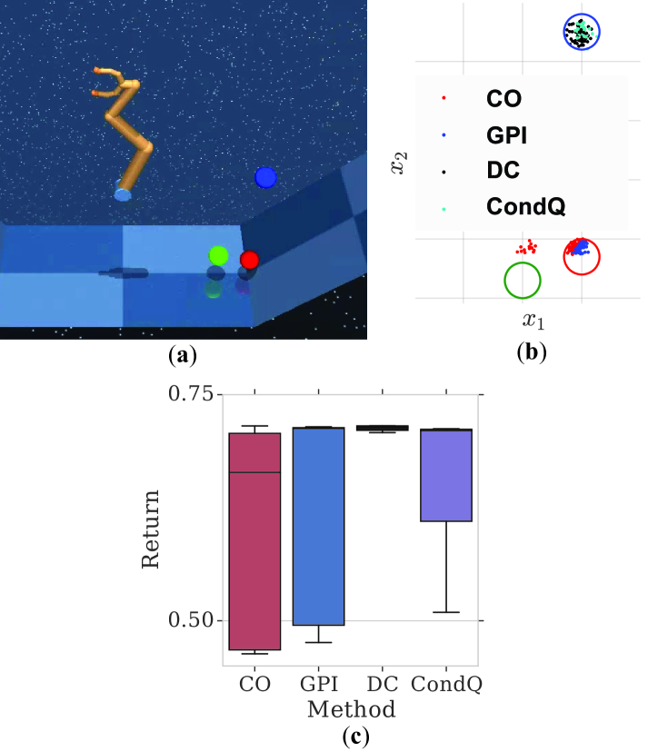
Figure 3: “Tricky” task with planar manipulator. (a) The “tricky” tasks with a 5D torque-controlled planar manipulator. The training tasks consists of (mutually exclusive) rewards of (1,0),(0,1)1001(1,0),(0,1) when the finger is at the green and red targets respectively and reward (0.75,0.75)0.750.75(0.75,0.75) at the blue target. (b) Finger position at the end of the trajectories starting from randomly sampled start states) for the transfer task with circles indicating the positions of the targets. DC and CondQ trajectories reach towards the blue target (the optimal solution) while CO and GPI trajectories primarily reach towards one of the suboptimal partial solutions. (c) Box plot of returns on the transfer tasks, DC outperforms other methods. Additional details in supplementary figure 7.

4.4 Sampling Compositional Policies

During transfer we need to sample from the Boltzmann policy defined by our estimate of the transfer action-value Qbsubscript𝑄𝑏Q_{b} (the estimate is computed using the methods we enumerated above). We wish to avoid needing to, offline, learn a new proposal or sampling distribution first (which is the approach employed by Haarnoja et al. (2018a)).

As outlined earlier (and detailed in appendix C.3), we chose the proposal distributions so that the product of proposals is tractable, meaning we can sample from qbij(a|s)(qθqi(a|s))b(qθj(a|s))(1b)proportional-tosubscriptsuperscript𝑞𝑖𝑗𝑏conditional𝑎𝑠superscriptsubscriptsuperscript𝑞𝑖subscript𝜃𝑞conditional𝑎𝑠𝑏superscriptsubscriptsuperscript𝑞𝑗𝜃conditional𝑎𝑠1𝑏q^{ij}_{b}(a|s)\propto(q^{i}_{\theta_{q}}(a|s))^{b}(q^{j}_{\theta}(a|s))^{(1-b)}. This is a good proposal distribution when the CO bias is low, since QbCOsubscriptsuperscript𝑄𝐶𝑂𝑏Q^{CO}_{b} defines a Boltzmann policy which is the product of the base policies111πbCO(a|s)exp1αQCO(s,a)=exp(1α(Q1(s,a)+Q2(s,a))=π1(a|s)π2(a|s)\pi^{CO}_{b}(a|s)\propto\exp\frac{1}{\alpha}Q^{CO}(s,a)=\exp(\frac{1}{\alpha}(Q^{1}(s,a)+Q^{2}(s,a))=\pi_{1}(a|s)\pi_{2}(a|s).. However, when Cb(s,a)subscriptsuperscript𝐶𝑏𝑠𝑎C^{\infty}_{b}(s,a) is large, meaning the CO bias is large, qijsuperscript𝑞𝑖𝑗q^{ij} may not be a good proposal, as we show in the experiments. In this case none of the existing proposal distributions may be a good fit. Therefore we sample from a mixture distribution of all policies, all policy products and the uniform distribution, with the hope that at least one component of this mixture will be sampling from high-value parts of the action space.

pb(a|s)14(qθqi(a|s)+qθqj(a|s)+qbij(a|s)+1𝒱A)subscript𝑝𝑏conditional𝑎𝑠14superscriptsubscript𝑞subscript𝜃𝑞𝑖conditional𝑎𝑠superscriptsubscript𝑞subscript𝜃𝑞𝑗conditional𝑎𝑠superscriptsubscript𝑞𝑏𝑖𝑗conditional𝑎𝑠1superscript𝒱𝐴\displaystyle\textstyle p_{b}(a|s)\equiv\frac{1}{4}(q_{\theta_{q}}^{i}(a|s)+q_{\theta_{q}}^{j}(a|s)+q_{b}^{ij}(a|s)+\frac{1}{\mathcal{V}^{A}}) (13)

where 𝒱Asuperscript𝒱𝐴\mathcal{V}^{A} is the volume of the action space. Empirically, we find this is sufficient to result in good performance during transfer. The transfer algorithm is given in supplementary algorithm 2.

5 Experiments

5.1 Discrete, tabular environment

We first provide some illustrative tabular cases of compositional transfer. These highlight situations in which GPI and CO transfer can perform poorly (Figure 1). As expected from theory, we find that GPI performs well when the optimal transfer policy is close to one of the existing policies; CO performs well when both subtask policies are compatible, meaning there is some part of the action space that has a high likelihood under both policies. The task we refer to as “tricky” is illustrative of challenging tasks we will focus on in the next section, namely scenarios in which the optimal policy for the transfer task does not resemble either existing policy: In the grid world non-overlapping rewards for each task are provided in one corner of the grid world, while lower value overlapping rewards are provided in the other corner (cf. Fig. 1). As a consequence both GPI and CO perform poorly while DC performs well in all cases.
Refer to caption
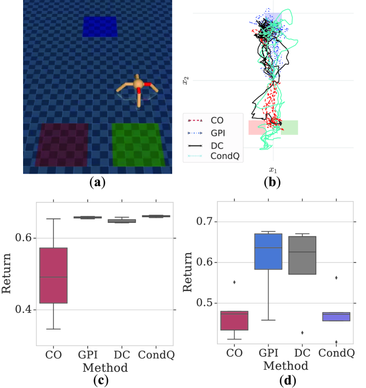
Figure 4: “Tricky” task with mobile bodies. “Tricky” task with two bodies: a 3 DOF jumping ball (supplementary figure 8a) and (a) 8 DOF ant (both torque controlled). The task has rewards (1,0),(0,1)1001(1,0),(0,1) in the green and red boxes respectively and (0.75,0.75)0.750.75(0.75,0.75) in the blue square. (b) Sampled trajectories of the ant on the transfer task (b=12𝑏12b=\frac{1}{2}) starting from a neutral position. GPI and DC almost always go to the blue square (optimal), CondQ and CO do not. Box plot of returns for the jumping ball (c) and ant (d) when started in the center position. CO does not recover a good transfer policy for the compositional task while the other approaches largely succeed, although CondQ does not learn a good policy on the ant. Additional details in supplementary figure 8.

5.2 Continuous action spaces

In the tabular environments we demonstrated some challenging “tricky” transfer tasks that previous methods perform poorly on. Here, we test our approach on continuous control tasks with the same challenging properties. We train max-ent policies to solve individual tasks and then compare transfer performance using the different approaches. All approaches use the same experience, proposal distributions and base policies.

Figure 2 examines the transfer policies in detail in a simple point-mass version of the “tricky” tasks and shows how the estimated Cbsubscriptsuperscript𝐶𝑏C^{\infty}_{b} corrects QCOsuperscript𝑄𝐶𝑂Q^{CO} and results in a qualitatively better transfer policy.

We now examine conceptually similar tasks in more difficult domains: a 5 DOF planar manipulator reaching task (figure 3), 3 DOF jumping ball and 8 DOF ant (figure 4). We see that DC recovers a qualitatively better policy in all cases. The performance of GPI depends noticeably on the choice of α𝛼\alpha. DC-Cheap, which is a simpler heuristic, performs almost as well as DC in the tasks we consider except for the point mass task. When bounded by GPI (DC-Cheap+GPI) it performs well for the point mass task as well, suggesting these heuristics may be sufficient in some cases222 Videos of the tasks and supplementary information at https://tinyurl.com/yaplfwaq. .

We focused on “tricky” tasks as they are a particularly challenging form of transfer. There are two other cases we considered in the tabular analysis. One: when the base tasks are compatible, CO performs well. We expect that DC would also perform well in this situation since, in this case, the correction term Cbsuperscriptsubscript𝐶𝑏C_{b}^{\infty} that DC must learn is inconsequential (CO is equivalent to assuming Cb=0superscriptsubscript𝐶𝑏0C_{b}^{\infty}=0). Two: At the other extreme, supplementary figure 9 demonstrates on a task with incompatible base tasks (i.e. Cbsuperscriptsubscript𝐶𝑏C_{b}^{\infty} is large and potentially challenging to learn), DC continues to perform as well as GPI, slightly better than CondQ and much better than CO. In principle, without function approximator error, DC always recovers the optimal policy during transfer. These experiments provide empirical evidence that our approximate algorithm performs well in a range of situations.

6 Discussion

We have presented two approaches to transfer learning via convex combinations of rewards in the maximum entropy framework: max-ent GPI and DC. We have shown that, under standard assumptions, the max-ent GPI policy performs at least as well as its component policies, and that DC recovers the optimal transfer policy. Todorov (2009) and (Pan et al., 2015; Saxe et al., 2017; van Niekerk et al., 2018) previously considered optimal composition of max-ent policies. However, these approaches require stronger assumptions about the class of MDPs. By contrast, DC does not restrict the class of MDPs and learns how compatible policies are, allowing approximate recovery of optimal transfer policies both when the component rewards are jointly achievable (AND), and when only one sub-goal can be achieved (OR).

We have compared our methods with conditional action-value functions (CondQ) (Schaul et al., 2015, e.g.) and optimistic policy combination (Haarnoja et al., 2018a). Further, we have presented AISBP, a practical algorithm for training DC and max-ent GPI models in continuous action spaces using adaptive importance sampling. We have compared these approaches, along with heuristic approximations of DC, and demonstrated that DC recovers an approximately optimal policy during transfer across a variety of high-dimensional control tasks. Empirically we have found CondQ may be harder to learn than DC, and it requires additional observation of ϕitalic-ϕ\phi during training.

Acknowledgements

We thank Alexander Pritzel, Alistair Muldal, Dhruva Tirumala, Siqi Liu and the rest of the DeepMind team for helpful discussions and assistance with this work.

References

  • Adolph et al. (2012) Adolph, K. E., Cole, W. G., Komati, M., Garciaguirre, J. S., Badaly, D., Lingeman, J. M., Chan, G. L., and Sotsky, R. B. How do you learn to walk? thousands of steps and dozens of falls per day. Psychological science, 23(11):1387–1394, 2012.
  • Andrychowicz et al. (2017) Andrychowicz, M., Wolski, F., Ray, A., Schneider, J., Fong, R., Welinder, P., McGrew, B., Tobin, J., Abbeel, O. P., and Zaremba, W. Hindsight experience replay. In Advances in Neural Information Processing Systems, pp. 5048–5058, 2017.
  • Baird (1994) Baird, L. C. Reinforcement learning in continuous time: Advantage updating. In Neural Networks, 1994. IEEE World Congress on Computational Intelligence., 1994 IEEE International Conference on, volume 4, pp. 2448–2453. IEEE, 1994.
  • Barreto et al. (2017) Barreto, A., Dabney, W., Munos, R., Hunt, J. J., Schaul, T., van Hasselt, H. P., and Silver, D. Successor features for transfer in reinforcement learning. In Advances in neural information processing systems, pp. 4055–4065, 2017.
  • Barreto et al. (2018) Barreto, A., Borsa, D., Quan, J., Schaul, T., Silver, D., Hessel, M., Mankowitz, D., Zidek, A., and Munos, R. Transfer in deep reinforcement learning using successor features and generalised policy improvement. In Proceedings of the International Conference on Machine Learning, pp.  501–510, 2018.
  • Clevert et al. (2015) Clevert, D.-A., Unterthiner, T., and Hochreiter, S. Fast and accurate deep network learning by exponential linear units (elus). arXiv preprint arXiv:1511.07289, 2015.
  • Dayan (1993) Dayan, P. Improving generalization for temporal difference learning: The successor representation. Neural Computation, 5(4):613–624, 1993.
  • Fox et al. (2016) Fox, R., Pakman, A., and Tishby, N. Taming the noise in reinforcement learning via soft updates. In Proceedings of the Thirty-Second Conference on Uncertainty in Artificial Intelligence, UAI’16, pp.  202–211, Arlington, Virginia, United States, 2016. AUAI Press. ISBN 978-0-9966431-1-5. URL http://dl.acm.org/citation.cfm?id=3020948.3020970.
  • Gil et al. (2013) Gil, M., Alajaji, F., and Linder, T. Rényi divergence measures for commonly used univariate continuous distributions. Information Sciences, 249:124–131, 2013.
  • Gu et al. (2015) Gu, S., Ghahramani, Z., and Turner, R. E. Neural adaptive sequential monte carlo. In Advances in Neural Information Processing Systems, pp. 2629–2637, 2015.
  • Haarnoja et al. (2017) Haarnoja, T., Tang, H., Abbeel, P., and Levine, S. Reinforcement learning with deep energy-based policies. In International Conference on Machine Learning, 2017.
  • Haarnoja et al. (2018a) Haarnoja, T., Pong, V., Zhou, A., Dalal, M., Abbeel, P., and Levine, S. Composable deep reinforcement learning for robotic manipulation. In International Conference on Robotics and Automation, 2018a.
  • Haarnoja et al. (2018b) Haarnoja, T., Zhou, A., Abbeel, P., and Levine, S. Soft actor-critic: Off-policy maximum entropy deep reinforcement learning with a stochastic actor. In International Conference on Machine Learning, 2018b.
  • Haith & Krakauer (2013) Haith, A. M. and Krakauer, J. W. Model-based and model-free mechanisms of human motor learning. In Progress in motor control, pp.  1–21. Springer, 2013.
  • Harmon et al. (1995) Harmon, M. E., Baird III, L. C., and Klopf, A. H. Advantage updating applied to a differential game. In Advances in neural information processing systems, pp. 353–360, 1995.
  • Kalashnikov et al. (2018) Kalashnikov, D., Irpan, A., Pastor, P., Ibarz, J., Herzog, A., Jang, E., Quillen, D., Holly, E., Kalakrishnan, M., Vanhoucke, V., et al. Qt-opt: Scalable deep reinforcement learning for vision-based robotic manipulation. arXiv preprint arXiv:1806.10293, 2018.
  • Kappen (2005) Kappen, H. J. Path integrals and symmetry breaking for optimal control theory. Journal of statistical mechanics: theory and experiment, 2005(11):P11011, 2005.
  • Lillicrap et al. (2015) Lillicrap, T. P., Hunt, J. J., Pritzel, A., Heess, N., Erez, T., Tassa, Y., Silver, D., and Wierstra, D. Continuous control with deep reinforcement learning. arXiv preprint arXiv:1509.02971, 2015.
  • Mnih et al. (2015) Mnih, V., Kavukcuoglu, K., Silver, D., Rusu, A. A., Veness, J., Bellemare, M. G., Graves, A., Riedmiller, M., Fidjeland, A. K., Ostrovski, G., et al. Human-level control through deep reinforcement learning. Nature, 518(7540):529, 2015.
  • Murphy (2012) Murphy, K. P. Machine Learning: A Probabilistic Perspective. The MIT Press, 2012. ISBN 0262018020, 9780262018029.
  • Pan et al. (2015) Pan, Y., Theodorou, E., and Kontitsis, M. Sample efficient path integral control under uncertainty. In Advances in Neural Information Processing Systems, pp. 2314–2322, 2015.
  • Precup et al. (1998) Precup, D., Sutton, R. S., and Singh, S. Theoretical results on reinforcement learning with temporally abstract options. In European conference on machine learning, pp.  382–393. Springer, 1998.
  • Saxe et al. (2017) Saxe, A. M., Earle, A. C., and Rosman, B. Hierarchy through composition with multitask LMDPs. In Precup, D. and Teh, Y. W. (eds.), Proceedings of the 34th International Conference on Machine Learning, volume 70 of Proceedings of Machine Learning Research, pp.  3017–3026, International Convention Centre, Sydney, Australia, 06–11 Aug 2017. PMLR. URL http://proceedings.mlr.press/v70/saxe17a.html.
  • Schaul et al. (2015) Schaul, T., Horgan, D., Gregor, K., and Silver, D. Universal value function approximators. In International Conference on Machine Learning, pp. 1312–1320, 2015.
  • Schrempf et al. (2005) Schrempf, O. C., Feiermann, O., and Hanebeck, U. D. Optimal mixture approximation of the product of mixtures. In International Conference on Information Fusion, volume 1, pp.  8–pp. IEEE, 2005.
  • Silver et al. (2016) Silver, D., Huang, A., Maddison, C. J., Guez, A., Sifre, L., Van Den Driessche, G., Schrittwieser, J., Antonoglou, I., Panneershelvam, V., Lanctot, M., et al. Mastering the game of go with deep neural networks and tree search. Nature, 529(7587):484, 2016.
  • Tassa et al. (2018) Tassa, Y., Doron, Y., Muldal, A., Erez, T., Li, Y., Casas, D. d. L., Budden, D., Abdolmaleki, A., Merel, J., Lefrancq, A., et al. Deepmind control suite. arXiv preprint arXiv:1801.00690, 2018.
  • Todorov (2009) Todorov, E. Compositionality of optimal control laws. In Advances in Neural Information Processing Systems, pp. 1856–1864, 2009.
  • Todorov et al. (2012) Todorov, E., Erez, T., and Tassa, Y. Mujoco: A physics engine for model-based control. In Intelligent Robots and Systems (IROS), pp.  5026–5033. IEEE, 2012.
  • van Niekerk et al. (2018) van Niekerk, B., James, S., Earle, A., and Rosman, B. Will it blend? composing value functions in reinforcement learning. arXiv preprint arXiv:1807.04439, 2018.
  • Wang et al. (2015) Wang, Z., Schaul, T., Hessel, M., Van Hasselt, H., Lanctot, M., and De Freitas, N. Dueling network architectures for deep reinforcement learning. arXiv preprint arXiv:1511.06581, 2015.
  • Ziebart et al. (2008) Ziebart, B. D., Maas, A. L., Bagnell, J. A., and Dey, A. K. Maximum entropy inverse reinforcement learning. In AAAI, volume 8, pp.  1433–1438. Chicago, IL, USA, 2008.

Appendix A Proofs

A.1 Max-Ent Generalized Policy Improvement

See 3.1

For brevity we denote QmaxmaxiQisuperscript𝑄subscript𝑖superscript𝑄𝑖Q^{\max}\equiv\max_{i}Q^{i}. Define the soft Bellman operator associated with policy π𝜋\pi as

𝒯πQ(s,a)superscript𝒯𝜋𝑄𝑠𝑎\displaystyle\mathcal{T}^{\pi}Q(s,a) r(s,a,s)+γ𝔼p(s|s,a)[αH[π(|s)]+𝔼aπ(|s)[Q(s,a)]].\displaystyle\equiv r(s,a,s^{\prime})+\gamma\mathbb{E}_{p(s^{\prime}|s,a)}\left[\alpha H[\pi(\cdot|s^{\prime})]+\mathbb{E}_{a^{\prime}\sim\pi(\cdot|s^{\prime})}\left[Q(s^{\prime},a^{\prime})\right]\right].

Haarnoja et al. (2018b) have pointed out that the soft Bellman operator 𝒯πsuperscript𝒯𝜋\mathcal{T}^{\pi} corresponds to a conventional, “hard”, Bellman operator defined over the same MDP but with reward rπ(s,a,s)=r(s,a,s)+γα𝔼p(s|s,a)[H[π(|s)]]r_{\pi}(s,a,s^{\prime})=r(s,a,s^{\prime})+\gamma\alpha\mathbb{E}_{p(s^{\prime}|s,a)}\left[H[\pi(\cdot|s^{\prime})]\right]. Thus, as long as r(s,a,s)𝑟𝑠𝑎superscript𝑠r(s,a,s^{\prime}) and H[π(|s)]H[\pi(\cdot|s^{\prime})] are bounded, 𝒯πsuperscript𝒯𝜋\mathcal{T}^{\pi} is a contraction with Qπsuperscript𝑄𝜋Q^{\pi} as its fixed point. Applying 𝒯πsuperscript𝒯𝜋\mathcal{T}^{\pi} to Qmax(s,a)superscript𝑄𝑠𝑎Q^{\max}(s,a) we have:

𝒯πQmax(s,a)superscript𝒯𝜋superscript𝑄𝑠𝑎\displaystyle\mathcal{T}^{\pi}Q^{\max}(s,a) =r(s,a,s)+γ𝔼sp(|s,a),aπ(|s)[αlogπ(a|s)+Qmax(s,a)]\displaystyle=r(s,a,s^{\prime})+\gamma\mathbb{E}_{s^{\prime}\sim p(\cdot|s,a),a^{\prime}\sim\pi(\cdot|s^{\prime})}\left[-\alpha\log\pi(a^{\prime}|s^{\prime})+Q^{\max}(s^{\prime},a^{\prime})\right]
=r(s,a,s)+γ𝔼sp(|s,a),aπ(|s)[αlogexp(α1Qmax(s,a))Zπ(s)+Qmax(s,a)]\displaystyle=r(s,a,s^{\prime})+\gamma\mathbb{E}_{s^{\prime}\sim p(\cdot|s,a),a^{\prime}\sim\pi(\cdot|s^{\prime})}\left[-\alpha\log\dfrac{\exp(\alpha^{-1}Q^{\max}(s^{\prime},a^{\prime}))}{Z^{\pi}(s^{\prime})}+Q^{\max}(s^{\prime},a^{\prime})\right]
=r(s,a,s)+γ𝔼sp(|s,a)[αlogZπ(s)].\displaystyle=r(s,a,s^{\prime})+\gamma\mathbb{E}_{s^{\prime}\sim p(\cdot|s,a)}\left[\alpha\log Z^{\pi}(s^{\prime})\right].

Similarly, if we apply 𝒯πisuperscript𝒯subscript𝜋𝑖\mathcal{T}^{\pi_{i}}, the soft Bellman operator induced by policy πisubscript𝜋𝑖\pi_{i}, to Qmax(s,a)superscript𝑄𝑠𝑎Q^{\max}(s,a), we obtain:

𝒯πiQmax(s,a)superscript𝒯subscript𝜋𝑖superscript𝑄𝑠𝑎\displaystyle\mathcal{T}^{\pi_{i}}Q^{\max}(s,a) =r(s,a,s)+γ𝔼sp(|s,a),aπi(|s)[αlogπi(a|s)+Qmax(s,a)].\displaystyle=r(s,a,s^{\prime})+\gamma\mathbb{E}_{s^{\prime}\sim p(\cdot|s,a),a^{\prime}\sim\pi_{i}(\cdot|s^{\prime})}\left[-\alpha\log\pi_{i}(a^{\prime}|s^{\prime})+Q^{\max}(s^{\prime},a^{\prime})\right].

We now note that the Kullback-Leibler divergence between πisubscript𝜋𝑖\pi_{i} and π𝜋\pi can be written as

DKL(πi(|s)π(|s))\displaystyle D_{\mathrm{KL}}({\pi_{i}(\cdot|s)}\|{\pi(\cdot|s)}) =𝔼aπi(|s)[logπi(a|s)logπ(a|s)]\displaystyle=\mathbb{E}_{a\sim\pi_{i}(\cdot|s)}\left[\log\pi_{i}(a|s)-\log\pi(a|s)\right]
=𝔼aπi(|s)[logπi(a|s)1αQmax(s,a)+logZπ(s)].\displaystyle=\mathbb{E}_{a\sim\pi_{i}(\cdot|s)}\left[\log\pi_{i}(a|s)-\frac{1}{\alpha}Q^{\max}(s,a)+\log Z^{\pi}(s)\right].

The quantity above, which is always nonnegative, will be useful in the subsequent derivations. Next we write

𝒯πQmax(s,a)𝒯πiQmax(s,a)superscript𝒯𝜋superscript𝑄𝑠𝑎superscript𝒯subscript𝜋𝑖superscript𝑄𝑠𝑎\displaystyle\mathcal{T}^{\pi}Q^{\max}(s,a)-\mathcal{T}^{\pi_{i}}Q^{\max}(s,a) =γ𝔼sp(|s,a)[αlogZπ(s)𝔼aπi(|s)[αlogπi(a|s)+Qmax(s,a)]]\displaystyle=\gamma\mathbb{E}_{s^{\prime}\sim p(\cdot|s,a)}\left[\alpha\log Z^{\pi}(s^{\prime})-\mathbb{E}_{a^{\prime}\sim\pi_{i}(\cdot|s^{\prime})}[-\alpha\log\pi_{i}(a^{\prime}|s^{\prime})+Q^{\max}(s^{\prime},a^{\prime})]\right]
=γ𝔼sp(|s,a)[𝔼aπi(|s)[αlogZπ(s)+αlogπi(a|s)Qmax(s,a)]]\displaystyle=\gamma\mathbb{E}_{s^{\prime}\sim p(\cdot|s,a)}\left[\mathbb{E}_{a^{\prime}\sim\pi_{i}(\cdot|s^{\prime})}[\alpha\log Z^{\pi}(s^{\prime})+\alpha\log\pi_{i}(a^{\prime}|s^{\prime})-Q^{\max}(s^{\prime},a^{\prime})]\right]
=γ𝔼sp(|s,a)[αDKL(πi(|s)π(|s))]\displaystyle=\gamma\mathbb{E}_{s^{\prime}\sim p(\cdot|s,a)}\left[\alpha D_{\mathrm{KL}}({\pi_{i}(\cdot|s^{\prime})}\|{\pi(\cdot|s^{\prime})})\right]
0.absent0\displaystyle\geq 0. (14)

From (A.1) we have that

𝒯πQmax(s,a)𝒯πiQmax(s,a)𝒯πiQi(s,a)=Qi(s,a) for all i.superscript𝒯𝜋superscript𝑄𝑠𝑎superscript𝒯subscript𝜋𝑖superscript𝑄𝑠𝑎superscript𝒯subscript𝜋𝑖superscript𝑄𝑖𝑠𝑎superscript𝑄𝑖𝑠𝑎 for all 𝑖\displaystyle\mathcal{T}^{\pi}Q^{\max}(s,a)\geq\mathcal{T}^{\pi_{i}}Q^{\max}(s,a)\geq\mathcal{T}^{\pi_{i}}Q^{i}(s,a)=Q^{i}(s,a)\;\text{ for all }i.

Using the contraction and monotonicity of the soft Bellman operator 𝒯πsuperscript𝒯𝜋\mathcal{T}^{\pi} we have

Qπ(s,a)superscript𝑄𝜋𝑠𝑎\displaystyle Q^{\pi}(s,a) =limk(𝒯π)kQmax(s,a)Qi(s,a) for all i.absentsubscript𝑘superscriptsuperscript𝒯𝜋𝑘superscript𝑄𝑠𝑎superscript𝑄𝑖𝑠𝑎 for all 𝑖\displaystyle=\lim_{k\rightarrow\infty}(\mathcal{T}^{\pi})^{k}Q^{\max}(s,a)\geq Q^{i}(s,a)\;\text{ for all }i.

We have just showed (5). In order to show (6), we note that

Vπ(s)superscript𝑉𝜋𝑠\displaystyle V^{\pi}(s) αH[π(|s)]+𝔼aπ[Qπ(s,a)]\displaystyle\equiv\alpha H[\pi(\cdot|s)]+\mathbb{E}_{a\sim\pi}\left[Q^{\pi}(s,a)\right]
αH[π(|s)]+𝔼aπ[Qmax(s,a)]\displaystyle\geq\alpha H[\pi(\cdot|s)]+\mathbb{E}_{a\sim\pi}\left[Q^{\max}(s,a)\right]
=αlogZπ(s).absent𝛼superscript𝑍𝜋𝑠\displaystyle=\alpha\log Z^{\pi}(s). (15)

Similarly, we have, for all i𝑖i,

Vi(s)superscript𝑉𝑖𝑠\displaystyle V^{i}(s) =𝔼aπi(|s)[Qi(s,a)αlogπi(a|s)]\displaystyle=\mathbb{E}_{a\sim\pi_{i}(\cdot|s)}\left[Q^{i}(s,a)-\alpha\log\pi_{i}(a|s)\right]
𝔼aπi(|s)[Qmax(s,a)αlogπi(a|s)]\displaystyle\leq\mathbb{E}_{a\sim\pi_{i}(\cdot|s)}\left[Q^{\max}(s,a)-\alpha\log\pi_{i}(a|s)\right]
=αlogZπ(s)αDKL(πi(|s)π(|s))\displaystyle=\alpha\log Z^{\pi}(s)-\alpha D_{\mathrm{KL}}({\pi_{i}(\cdot|s)}\|{\pi(\cdot|s)})
αlogZπ(s).absent𝛼superscript𝑍𝜋𝑠\displaystyle\leq\alpha\log Z^{\pi}(s). (16)

The bound (6) follows from (A.1) and (A.1).

A.2 DC Proof

See 3.2

We follow a similar approach to (Haarnoja et al., 2018a) but without making approximations and generalizing to all convex combinations.

First note that since πisubscript𝜋𝑖\pi_{i} and πjsubscript𝜋𝑗\pi_{j} are optimal then πi(a|s)=exp(1α(Qi(s,a)Vi(s)))subscript𝜋𝑖conditional𝑎𝑠1𝛼superscript𝑄𝑖𝑠𝑎superscript𝑉𝑖𝑠\pi_{i}(a|s)=\exp({\frac{1}{\alpha}(Q^{i}(s,a)-V^{i}(s))}).

For brevity we use s𝑠s and ssuperscript𝑠s^{\prime} notation rather than writing the time index.

Define

Qb(0)(s,a)subscriptsuperscript𝑄0𝑏𝑠𝑎\displaystyle Q^{(0)}_{b}(s,a) bQi(s,a)+(1b)Qj(s,a)absent𝑏superscript𝑄𝑖𝑠𝑎1𝑏superscript𝑄𝑗𝑠𝑎\displaystyle\equiv bQ^{i}(s,a)+(1-b)Q^{j}(s,a) (17)
C(0)(s,a)superscript𝐶0𝑠𝑎\displaystyle C^{(0)}(s,a) 0absent0\displaystyle\equiv 0 (18)

and consider soft Q-iteration on rbsubscript𝑟𝑏r_{b} starting from Qb(0)subscriptsuperscript𝑄0𝑏Q^{(0)}_{b}. We prove, inductively, that at each iteration Qb(k+1)=bQi(s,a)+(1b)Qj(s,a)C(k+1)(s,a)subscriptsuperscript𝑄𝑘1𝑏𝑏superscript𝑄𝑖𝑠𝑎1𝑏superscript𝑄𝑗𝑠𝑎superscript𝐶𝑘1𝑠𝑎Q^{(k+1)}_{b}=bQ^{i}(s,a)+(1-b)Q^{j}(s,a)-C^{(k+1)}(s,a).

This is true by definition for k=0𝑘0k=0.

Qb(k+1)(s,a)superscriptsubscript𝑄𝑏𝑘1𝑠𝑎\displaystyle Q_{b}^{(k+1)}(s,a) =rb(s,a)+γα𝔼p(s|s,a)[log𝒜exp1αQb(k)(s,a)𝑑a]absentsubscript𝑟𝑏𝑠𝑎𝛾𝛼subscript𝔼𝑝conditionalsuperscript𝑠𝑠𝑎delimited-[]subscript𝒜1𝛼superscriptsubscript𝑄𝑏𝑘superscript𝑠superscript𝑎differential-dsuperscript𝑎\displaystyle=r_{b}(s,a)+\gamma\alpha\mathbb{E}_{p(s^{\prime}|s,a)}\left[\log\int_{\mathcal{A}}\exp\frac{1}{\alpha}Q_{b}^{(k)}(s^{\prime},a^{\prime})da^{\prime}\right] (19)
=rb(s,a)+absentlimit-fromsubscript𝑟𝑏𝑠𝑎\displaystyle=r_{b}(s,a)+ (20)
γα𝔼p(s|s,a)[log𝒜exp(1α(bQi(s,a)+(1b)Qj(s,a)C(k)(s,a)))𝑑a]𝛾𝛼subscript𝔼𝑝conditionalsuperscript𝑠𝑠𝑎delimited-[]subscript𝒜1𝛼𝑏superscript𝑄𝑖superscript𝑠superscript𝑎1𝑏superscript𝑄𝑗superscript𝑠superscript𝑎superscript𝐶𝑘superscript𝑠superscript𝑎differential-dsuperscript𝑎\displaystyle\gamma\alpha\mathbb{E}_{p(s^{\prime}|s,a)}\left[\log\int_{\mathcal{A}}\exp(\frac{1}{\alpha}(bQ^{i}(s^{\prime},a^{\prime})+(1-b)Q^{j}(s^{\prime},a^{\prime})-C^{(k)}(s^{\prime},a^{\prime})))da^{\prime}\right]
=rb(s,a)+absentlimit-fromsubscript𝑟𝑏𝑠𝑎\displaystyle=r_{b}(s,a)+ (21)
𝔼p(s|s,a)[bVi(s)+(1b)Vj(s)+αlog𝒜exp(blogπi(a|s)+(1b)logπj(a|s)1αC(k)(s,a))𝑑a]subscript𝔼𝑝conditionalsuperscript𝑠𝑠𝑎delimited-[]𝑏superscript𝑉𝑖superscript𝑠1𝑏superscript𝑉𝑗superscript𝑠𝛼subscript𝒜𝑏subscript𝜋𝑖conditionalsuperscript𝑎superscript𝑠1𝑏subscript𝜋𝑗conditionalsuperscript𝑎superscript𝑠1𝛼superscript𝐶𝑘superscript𝑠superscript𝑎differential-dsuperscript𝑎\displaystyle\mathbb{E}_{p(s^{\prime}|s,a)}\left[bV^{i}(s^{\prime})+(1-b)V^{j}(s^{\prime})+\alpha\log\int_{\mathcal{A}}\exp(b\log\pi_{i}(a^{\prime}|s^{\prime})+(1-b)\log\pi_{j}(a^{\prime}|s^{\prime})-\frac{1}{\alpha}C^{(k)}(s^{\prime},a^{\prime}))da^{\prime}\right]
=bQi(s,a)+(1b)Qj(s,a)+absent𝑏superscript𝑄𝑖𝑠𝑎limit-from1𝑏superscript𝑄𝑗𝑠𝑎\displaystyle=bQ^{i}(s,a)+(1-b)Q^{j}(s,a)+ (22)
αγ𝔼p(s|s,a)[log𝒜exp(blogπ1(a|s)+(1b)logπ2(a|s)1αC(k)(s,a))𝑑a]𝛼𝛾subscript𝔼𝑝conditionalsuperscript𝑠𝑠𝑎delimited-[]subscript𝒜𝑏subscript𝜋1conditionalsuperscript𝑎superscript𝑠1𝑏subscript𝜋2conditionalsuperscript𝑎superscript𝑠1𝛼superscript𝐶𝑘superscript𝑠superscript𝑎differential-dsuperscript𝑎\displaystyle\alpha\gamma\mathbb{E}_{p(s^{\prime}|s,a)}\left[\log\int_{\mathcal{A}}\exp(b\log\pi_{1}(a^{\prime}|s^{\prime})+(1-b)\log\pi_{2}(a^{\prime}|s^{\prime})-\frac{1}{\alpha}C^{(k)}(s^{\prime},a^{\prime}))da^{\prime}\right]
=bQi(s,a)+(1b)Qi(s,a)Cb(k+1)(s,a).absent𝑏superscript𝑄𝑖𝑠𝑎1𝑏superscript𝑄𝑖𝑠𝑎subscriptsuperscript𝐶𝑘1𝑏𝑠𝑎\displaystyle=bQ^{i}(s,a)+(1-b)Q^{i}(s,a)-C^{(k+1)}_{b}(s,a). (23)

Since soft Q-iteration converges to the α𝛼\alpha max-ent optimal soft Q𝑄Q then at the limit kinf𝑘infimumk\rightarrow\inf theorem 3.2 holds.

One can get an intuition for Cb(s,a)subscriptsuperscript𝐶𝑏𝑠𝑎C^{\infty}_{b}(s,a) by noting that

Cb(1)(s,a)=γα𝔼p(s|s,a)[(1b)Db(π1(|s)π2(|s))]\displaystyle C^{(1)}_{b}(s,a)=\gamma\alpha\mathbb{E}_{p(s^{\prime}|s,a)}\left[(1-b)\operatorname{D}_{b}\left(\pi_{1}(\cdot|s)\middle\|\pi_{2}(\cdot|s)\right)\right] (24)

where DbsubscriptD𝑏\operatorname{D}_{b} is the Rényi divergence of order b𝑏b. Cb(s,a)subscriptsuperscript𝐶𝑏𝑠𝑎C^{\infty}_{b}(s,a) can be seen as the discount sum of divergences, weighted by the unnormalized product distribution π1(a|s)bπ2(a|s)1bsubscript𝜋1superscriptconditional𝑎𝑠𝑏subscript𝜋2superscriptconditional𝑎𝑠1𝑏\pi_{1}(a|s)^{b}\pi_{2}(a|s)^{1-b}.

A.3 N𝑁N policies

It is possible to extend Theorem 3.2 to the case with N𝑁N policies in a straightforward way.

Theorem A.1 (Multi-policy DC Optimality)

Let π1,π2,,πNsubscript𝜋1subscript𝜋2subscript𝜋𝑁\pi_{1},\pi_{2},...,\pi_{N} be α𝛼\alpha max-ent optimal policies for tasks with rewards r1,r2,,rNsubscript𝑟1subscript𝑟2subscript𝑟𝑁r_{1},r_{2},...,r_{N} with max-ent action-value functions Q1,Q2,,QNsuperscript𝑄1superscript𝑄2superscript𝑄𝑁Q^{1},Q^{2},...,Q^{N}.

Define C𝐰(st,at)subscriptsuperscript𝐶𝐰subscript𝑠𝑡subscript𝑎𝑡C^{\infty}_{\mathbf{w}}(s_{t},a_{t}) as the fixed point of

C𝐰(k+1)(st,at)=αγ𝔼p(st+1|st,at)[log𝒜(i=1Nπi(at+1|st+1)wi)exp(1αC𝐰(k)(st+1,at+1))𝑑at+1]subscriptsuperscript𝐶𝑘1𝐰subscript𝑠𝑡subscript𝑎𝑡𝛼𝛾subscript𝔼𝑝conditionalsubscript𝑠𝑡1subscript𝑠𝑡subscript𝑎𝑡delimited-[]subscript𝒜superscriptsubscriptproduct𝑖1𝑁subscript𝜋𝑖superscriptconditionalsubscript𝑎𝑡1subscript𝑠𝑡1subscript𝑤𝑖1𝛼subscriptsuperscript𝐶𝑘𝐰subscript𝑠𝑡1subscript𝑎𝑡1differential-dsubscript𝑎𝑡1\displaystyle\textstyle C^{(k+1)}_{\mathbf{w}}(s_{t},a_{t})=-\alpha\gamma\mathbb{E}_{p(s_{t+1}|s_{t},a_{t})}\left[\log\int_{\mathcal{A}}\left(\prod_{i=1}^{N}\pi_{i}(a_{t+1}|s_{t+1})^{w_{i}}\right)\exp(-\frac{1}{\alpha}C^{(k)}_{\mathbf{w}}(s_{t+1},a_{t+1}))da_{t+1}\right]

Given the conditions for Soft Q convergence, the max-ent optimal Q𝐰(s,a)subscriptsuperscript𝑄𝐰𝑠𝑎Q^{*}_{\mathbf{w}}(s,a) for the convex combination of rewards r𝐰=i=1Nriwisubscript𝑟𝐰superscriptsubscript𝑖1𝑁subscript𝑟𝑖subscript𝑤𝑖r_{\mathbf{w}}=\sum_{i=1}^{N}r_{i}w_{i} is

Q𝐰(s,a)=i=1NwiQi(s,a)C𝐰(s,a)subscriptsuperscript𝑄𝐰𝑠𝑎superscriptsubscript𝑖1𝑁subscript𝑤𝑖superscript𝑄𝑖𝑠𝑎subscriptsuperscript𝐶𝐰𝑠𝑎\displaystyle\textstyle Q^{*}_{\mathbf{w}}(s,a)=\sum_{i=1}^{N}w_{i}Q^{i}(s,a)-C^{\infty}_{\mathbf{w}}(s,a)
s𝒮,a𝒜,𝐰{𝐰|i=1Nwi=1andwi0}formulae-sequencefor-all𝑠𝒮formulae-sequence𝑎𝒜𝐰conditional-set𝐰superscriptsubscript𝑖1𝑁subscript𝑤𝑖1andsubscript𝑤𝑖0\displaystyle\forall s\in\mathcal{S},a\in\mathcal{A},\mathbf{w}\in\{\mathbf{w}|\sum_{i=1}^{N}w_{i}=1\>\>\>\mathrm{and}\>\>\>w_{i}\geq 0\}

Note that wisubscript𝑤𝑖w_{i} refers to component i𝑖i of the vector 𝐰isubscript𝐰𝑖\mathbf{w}_{i}.

The proof is very similar to the two reward case above.

Define

Q𝐰(0)i=1NwiQi(s,a)superscriptsubscript𝑄𝐰0superscriptsubscript𝑖1𝑁subscript𝑤𝑖superscript𝑄𝑖𝑠𝑎\displaystyle Q_{\mathbf{w}}^{(0)}\equiv\sum_{i=1}^{N}w_{i}Q^{i}(s,a) (25)
C𝐰(0)0superscriptsubscript𝐶𝐰00\displaystyle C_{\mathbf{w}}^{(0)}\equiv 0 (26)

and again consider soft Q-iteration on r𝐰subscript𝑟𝐰r_{\mathbf{w}}. We prove by induction that at each iteration

Q𝐰(k+1)(s,a)=i=1NwiQi(s,a)C𝐰(k+1)(s,a)subscriptsuperscript𝑄𝑘1𝐰𝑠𝑎superscriptsubscript𝑖1𝑁subscript𝑤𝑖superscript𝑄𝑖𝑠𝑎superscriptsubscript𝐶𝐰𝑘1𝑠𝑎\displaystyle Q^{(k+1)}_{\mathbf{w}}(s,a)=\sum_{i=1}^{N}w_{i}Q^{i}(s,a)-C_{\mathbf{w}}^{(k+1)}(s,a) (27)

Again, this is true by definition for k=0𝑘0k=0. Now we consider a step of Soft Q iteration

Q𝐰(k+1)superscriptsubscript𝑄𝐰𝑘1\displaystyle Q_{\mathbf{w}}^{(k+1)} =r𝐰(s,a)+γα𝔼p(s|s,a)[log𝒜exp1αQ𝐰(k)(s,a)𝑑a]absentsubscript𝑟𝐰𝑠𝑎𝛾𝛼subscript𝔼𝑝conditionalsuperscript𝑠𝑠𝑎delimited-[]subscript𝒜1𝛼subscriptsuperscript𝑄𝑘𝐰superscript𝑠superscript𝑎differential-dsuperscript𝑎\displaystyle=r_{\mathbf{w}}(s,a)+\gamma\alpha\mathbb{E}_{p(s^{\prime}|s,a)}\left[\log\int_{\mathcal{A}}\exp\frac{1}{\alpha}Q^{(k)}_{\mathbf{w}}(s^{\prime},a^{\prime})da^{\prime}\right] (28)
=r𝐰(s,a)+γα𝔼p(s|s,a)[log𝒜exp1α(i=1NwiQi(s,a)C𝐰(k)(s,a))𝑑a]absentsubscript𝑟𝐰𝑠𝑎𝛾𝛼subscript𝔼𝑝conditionalsuperscript𝑠𝑠𝑎delimited-[]subscript𝒜1𝛼superscriptsubscript𝑖1𝑁subscript𝑤𝑖superscript𝑄𝑖superscript𝑠superscript𝑎superscriptsubscript𝐶𝐰𝑘𝑠𝑎differential-dsuperscript𝑎\displaystyle=r_{\mathbf{w}}(s,a)+\gamma\alpha\mathbb{E}_{p(s^{\prime}|s,a)}\left[\log\int_{\mathcal{A}}\exp\frac{1}{\alpha}\left(\sum_{i=1}^{N}w_{i}Q^{i}(s^{\prime},a^{\prime})-C_{\mathbf{w}}^{(k)}(s,a)\right)da^{\prime}\right] (29)
=r𝐰(s,a)+γ𝔼p(s|s,a)[i=1NwiVi(s)+αlog𝒜exp(i=1Nwilogπi(a|s)1αC𝐰(k)(s,a))𝑑a]absentsubscript𝑟𝐰𝑠𝑎𝛾subscript𝔼𝑝conditionalsuperscript𝑠𝑠𝑎delimited-[]superscriptsubscript𝑖1𝑁subscript𝑤𝑖superscript𝑉𝑖superscript𝑠𝛼subscript𝒜superscriptsubscript𝑖1𝑁subscript𝑤𝑖subscript𝜋𝑖conditionalsuperscript𝑎superscript𝑠1𝛼subscriptsuperscript𝐶𝑘𝐰superscript𝑠superscript𝑎differential-dsuperscript𝑎\displaystyle=r_{\mathbf{w}}(s,a)+\gamma\mathbb{E}_{p(s^{\prime}|s,a)}\left[\sum_{i=1}^{N}w_{i}V^{i}(s^{\prime})+\alpha\log\int_{\mathcal{A}}\exp\left(\sum_{i=1}^{N}w_{i}\log\pi_{i}(a^{\prime}|s^{\prime})-\frac{1}{\alpha}C^{(k)}_{\mathbf{w}}(s^{\prime},a^{\prime})\right)da^{\prime}\right] (30)
=i=1NwiQi(s,a)+αγ𝔼p(s|s,a)[log𝒜exp(i=1Nwilogπi(a|s)1αC𝐰(k)(s,a))𝑑a]absentsuperscriptsubscript𝑖1𝑁subscript𝑤𝑖superscript𝑄𝑖𝑠𝑎𝛼𝛾subscript𝔼𝑝conditionalsuperscript𝑠𝑠𝑎delimited-[]subscript𝒜superscriptsubscript𝑖1𝑁subscript𝑤𝑖subscript𝜋𝑖conditionalsuperscript𝑎superscript𝑠1𝛼superscriptsubscript𝐶𝐰𝑘superscript𝑠superscript𝑎differential-dsuperscript𝑎\displaystyle=\sum_{i=1}^{N}w_{i}Q^{i}(s,a)+\alpha\gamma\mathbb{E}_{p(s^{\prime}|s,a)}\left[\log\int_{\mathcal{A}}\exp(\sum_{i=1}^{N}w_{i}\log\pi_{i}(a^{\prime}|s^{\prime})-\frac{1}{\alpha}C_{\mathbf{w}}^{(k)}(s^{\prime},a^{\prime}))da^{\prime}\right] (31)
=i=1NwiQi(s,a)C𝐰(k+1)(s,a)absentsuperscriptsubscript𝑖1𝑁subscript𝑤𝑖superscript𝑄𝑖𝑠𝑎superscriptsubscript𝐶𝐰𝑘1𝑠𝑎\displaystyle=\sum_{i=1}^{N}w_{i}Q^{i}(s,a)-C_{\mathbf{w}}^{(k+1)}(s,a) (32)

Since soft Q-iteration converges to the α𝛼\alpha max-ent optimal soft Q𝑄Q then Q𝐰(s,a)=i=1NwiQi(s,a)C𝐰(k+1)(s,a)subscriptsuperscript𝑄𝐰𝑠𝑎superscriptsubscript𝑖1𝑁subscript𝑤𝑖superscript𝑄𝑖𝑠𝑎subscriptsuperscript𝐶𝑘1𝐰𝑠𝑎Q^{*}_{\mathbf{w}}(s,a)=\sum_{i=1}^{N}w_{i}Q^{i}(s,a)-C^{(k+1)}_{\mathbf{w}}(s,a) for all s𝒮,a𝒜formulae-sequence𝑠𝒮𝑎𝒜s\in\mathcal{S},\>a\in\mathcal{A}.

Note that, in practice, estimating C𝐰subscriptsuperscript𝐶𝐰C^{\infty}_{\mathbf{w}} may be more challenging for larger N𝑁N. For compositions of many policies, GPI may be more practical.

Appendix B Theoretical properties of the composition methods

Method Optimal Bounded loss Requires ϕitalic-ϕ{\bm{\phi}} Requires f(s,a|b)𝑓𝑠conditional𝑎𝑏f(s,a|b)
CO
CondQ na
GPI
DC na
Table 1: Theoretical properties of different approaches to max-ent transfer. The methods compared are: CO, CondQ, max-ent GPI (over a fixed, finite set of policies), and DC. The columns indicate whether the transfer policy is optimal, the regret of the transfer policy is bounded, whether rewards for all tasks ϕbold-italic-ϕ{\bm{\phi}} need to be observed simultaneously during training and whether the method requires learning a function conditional on the transfer task b𝑏b, f(s,a|b)𝑓𝑠conditional𝑎𝑏f(s,a|b). DC is the only method that both recovers (in principle) the optimal policy and does not require observing ϕitalic-ϕ\phi during training.

Appendix C Algorithm details

C.1 Transfer algorithm

Load trained parameters θQsubscript𝜃𝑄\theta_{Q}, θqsubscript𝜃𝑞\theta_{q}, θ𝝍subscript𝜃𝝍\theta_{\bm{\psi}}, θCsubscript𝜃𝐶\theta_{C}, θQbsubscript𝜃subscript𝑄𝑏\theta_{Q_{b}}.
Accept transfer task parameter b𝑏b, transfer method𝑚𝑒𝑡𝑜𝑑absentmethod\in CO, GPI, DC, CondQ.
while testing do
     Importance sample transfer policy πb(a|s)exp1αQmethod(s,a)proportional-tosubscript𝜋𝑏conditional𝑎𝑠1𝛼superscript𝑄𝑚𝑒𝑡𝑜𝑑𝑠𝑎\pi_{b}(a|s)\propto\exp\frac{1}{\alpha}Q^{method}(s,a) with mixture proposal pb(a|s)θqsubscript𝑝𝑏subscriptconditional𝑎𝑠subscript𝜃𝑞p_{b}(a|s)_{\theta_{q}}.
end while
Algorithm 2 AISBP transfer algorithm

C.2 All losses and estimators

We use neural networks to parametrize all quantities. For each policy we learn an action-value QθQ(s,a)subscript𝑄subscript𝜃𝑄𝑠𝑎Q_{\theta_{Q}}(s,a), value VθV(s)subscript𝑉subscript𝜃𝑉𝑠V_{\theta_{V}}(s) and proposal distribution qθq(a|s)subscript𝑞subscript𝜃𝑞conditional𝑎𝑠q_{\theta_{q}}(a|s). We use target networks for the proposal distribution qθq(a|s)subscript𝑞superscriptsubscript𝜃𝑞conditional𝑎𝑠q_{\theta_{q}^{\prime}}(a|s) and value VθV(s)subscript𝑉superscriptsubscript𝜃𝑉𝑠V_{\theta_{V}^{\prime}}(s).

Here we enumerate all of the losses and their estimators. We use temporal difference (TD(0)) learning for all the RL losses, so all losses are valid off-policy. We use a replay buffer R𝑅R and learn by sampling minibatches of SARS tuples of size B𝐵B, we index over the batch dimension with l𝑙l and use slsubscriptsuperscript𝑠𝑙s^{\prime}_{l} to denote the state following slsubscript𝑠𝑙s_{l}, so the tuple consists of (sl,al,rl,sl)subscript𝑠𝑙subscript𝑎𝑙subscript𝑟𝑙superscriptsubscript𝑠𝑙(s_{l},a_{l},r_{l},s_{l}^{\prime}). For importance sampled estimators we sample N𝑁N actions for each state slsubscript𝑠𝑙s_{l} and use alksubscript𝑎𝑙𝑘a_{lk} to denote sample k𝑘k for state l𝑙l.

We learn a set of n𝑛n policies, one for each task in 𝒯𝒯\mathcal{T} indexed by i𝑖i. However, we write the losses for a single policy and drop i𝑖i for notational simplicity.

C.2.1 Proposal loss

The proposal loss minimizes the KL divergence between the Boltzmann distribution π(a|s)exp(12Q(s,a))proportional-to𝜋conditional𝑎𝑠12𝑄𝑠𝑎\pi(a|s)\propto\exp(\frac{1}{2}Q(s,a)) and the proposal distribution.

(θq)subscript𝜃𝑞\displaystyle\mathcal{L}(\theta_{q}) =𝔼R[𝔼aπ(|s)[logπ(a|st)logqθq(a|st)]]\displaystyle=\mathbb{E}_{R}\left[\mathbb{E}_{a\sim\pi(\cdot|s)}[\log\pi(a|s_{t})-\log q_{\theta_{q}}(a|s_{t})]\right] (33)

As described in the text, this loss is estimated using importance sampling with a mixture distribution p(a|s)𝑝conditional𝑎𝑠p(a|s) containing equally weighted components consisting of the target proposal distribution qθq(a|s)subscript𝑞superscriptsubscript𝜃𝑞conditional𝑎𝑠q_{\theta_{q}^{\prime}}(a|s) for all policies and the uniform distribution.

p(a|s)=1n+1(1V𝒜+i=1nqθqi(a|s))𝑝conditional𝑎𝑠1𝑛11superscript𝑉𝒜superscriptsubscript𝑖1𝑛subscriptsuperscript𝑞𝑖superscriptsubscript𝜃𝑞conditional𝑎𝑠\displaystyle p(a|s)=\frac{1}{n+1}\left(\frac{1}{V^{\mathcal{A}}}+\sum_{i=1}^{n}q^{i}_{\theta_{q}^{\prime}}(a|s)\right) (34)

where V𝒜superscript𝑉𝒜V^{\mathcal{A}} is the volume of the action space (which is always bounded in our case).

The proposal loss is estimated using self-normalized importance sampling

(θq)subscript𝜃𝑞\displaystyle\mathcal{L}(\theta_{q}) 1Bk=1Bl=1Nwkllogqθq(a|st),absent1𝐵superscriptsubscript𝑘1𝐵superscriptsubscript𝑙1𝑁subscript𝑤𝑘𝑙subscript𝑞subscript𝜃𝑞conditional𝑎subscript𝑠𝑡\displaystyle\approx-\frac{1}{B}\sum_{k=1}^{B}\sum_{l=1}^{N}w_{kl}\log q_{\theta_{q}}(a|s_{t}), (35)
wklsubscriptsuperscript𝑤𝑘𝑙\displaystyle w^{\prime}_{kl} =1α(QθQ(sk,akl))p(akl|sk);wkl=wklm=1Nwkm.formulae-sequenceabsent1𝛼subscript𝑄subscript𝜃𝑄subscript𝑠𝑘subscript𝑎𝑘𝑙𝑝conditionalsubscript𝑎𝑘𝑙subscript𝑠𝑘subscript𝑤𝑘𝑙subscript𝑤𝑘superscript𝑙superscriptsubscript𝑚1𝑁subscriptsuperscript𝑤𝑘𝑚\displaystyle=\frac{\frac{1}{\alpha}(Q_{\theta_{Q}}(s_{k},a_{kl}))}{p(a_{kl}|s_{k})};\>\>w_{kl}=\frac{w_{kl^{\prime}}}{\sum_{m=1}^{N}w^{\prime}_{km}}. (36)

C.2.2 Value loss

The soft value loss is

(θV)=subscript𝜃𝑉absent\displaystyle\textstyle\mathcal{L}(\theta_{V})= 𝔼R[12(VθV(st)αlog𝒜exp(1αQθQ(st,a))𝑑a)2]subscript𝔼𝑅delimited-[]12superscriptsubscript𝑉subscript𝜃𝑉subscript𝑠𝑡𝛼subscript𝒜1𝛼subscript𝑄subscript𝜃𝑄subscript𝑠𝑡𝑎differential-d𝑎2\displaystyle\mathbb{E}_{R}\left[\frac{1}{2}(V_{\theta_{V}}(s_{t})-\alpha\log\int_{\mathcal{A}}\exp(\frac{1}{\alpha}Q_{\theta_{Q}}(s_{t},a))da)^{2}\right] (37)

We estimate this using importance sampling with the proposal distribution qθq(a|s)subscript𝑞subscript𝜃𝑞conditional𝑎𝑠q_{\theta_{q}}(a|s) which is trying to fit the policy π𝜋\pi.

(θV)subscript𝜃𝑉\displaystyle\mathcal{L}(\theta_{V}) 12Bl=1B(VθV(sl)αlogZ)2absent12𝐵superscriptsubscript𝑙1𝐵superscriptsubscript𝑉subscript𝜃𝑉subscript𝑠𝑙𝛼𝑍2\displaystyle\approx\frac{1}{2B}\sum_{l=1}^{B}\left(V_{\theta_{V}}(s_{l})-\alpha\log Z\right)^{2} (38)
Z𝑍\displaystyle Z =[1Nk=1Nexp(1αQθQ(sl,alk))qθq(alk|sl)]absentdelimited-[]1𝑁superscriptsubscript𝑘1𝑁1𝛼subscript𝑄subscript𝜃𝑄subscript𝑠𝑙subscript𝑎𝑙𝑘subscript𝑞subscript𝜃𝑞conditionalsubscript𝑎𝑙𝑘subscript𝑠𝑙\displaystyle=\left[\frac{1}{N}\sum_{k=1}^{N}\frac{\exp(\frac{1}{\alpha}Q_{\theta_{Q}}(s_{l},a_{lk}))}{q_{\theta_{q}}(a_{lk}|s_{l})}\right] (39)

C.2.3 Action-value loss

The TD(0) loss for QθQsubscript𝑄subscript𝜃𝑄Q_{\theta_{Q}} is

(θQ)=subscript𝜃𝑄absent\displaystyle\mathcal{L}(\theta_{Q})= 𝔼R[12(QθQ(st,at)(r(st,at,st+1)+γVθV(st+1)))2]subscript𝔼𝑅delimited-[]12superscriptsubscript𝑄subscript𝜃𝑄subscript𝑠𝑡subscript𝑎𝑡𝑟subscript𝑠𝑡subscript𝑎𝑡subscript𝑠𝑡1𝛾subscript𝑉superscriptsubscript𝜃𝑉subscript𝑠𝑡12\displaystyle\mathbb{E}_{R}\left[\frac{1}{2}(Q_{\theta_{Q}}(s_{t},a_{t})-(r(s_{t},a_{t},s_{t+1})+\gamma V_{\theta_{V}^{\prime}}(s_{t+1})))^{2}\right] (40)

This does not require importance sampling to estimate and can be straightforwardly estimated as

(θQ)12Bl=1B(QθQ(sl,al)(rl+γVθV(s)))2subscript𝜃𝑄12𝐵superscriptsubscript𝑙1𝐵superscriptsubscript𝑄subscript𝜃𝑄subscript𝑠𝑙subscript𝑎𝑙subscript𝑟𝑙𝛾subscript𝑉superscriptsubscript𝜃𝑉superscript𝑠2\displaystyle\mathcal{L}(\theta_{Q})\approx\frac{1}{2B}\sum_{l=1}^{B}(Q_{\theta_{Q}}(s_{l},a_{l})-(r_{l}+\gamma V_{\theta_{V}^{\prime}}(s^{\prime})))^{2} (41)

The action-value is parametrized as an advantage function QθQ(s,a)=VθV(s)+AθA(s,a)subscript𝑄subscript𝜃𝑄𝑠𝑎subscript𝑉superscriptsubscript𝜃𝑉𝑠subscript𝐴subscript𝜃𝐴𝑠𝑎Q_{\theta_{Q}}(s,a)=V_{\theta_{V}^{\prime}}(s)+A_{\theta_{A}}(s,a).

C.2.4 State Dependent Successor Features loss

To facilitate max-ent GPI we learn successor features for each policy, both state-action dependent features 𝝍θ𝝍(s,a)subscript𝝍subscript𝜃𝝍𝑠𝑎{\bm{\psi}}_{\theta_{\bm{\psi}}}(s,a) and state-dependent 𝚼θ𝚼(s)subscript𝚼subscript𝜃𝚼𝑠{\bm{\Upsilon}}_{\theta_{\bm{\Upsilon}}}(s). As with value, we use a target network for the state-dependent features 𝚼θ𝚼(s)subscript𝚼superscriptsubscript𝜃𝚼𝑠{\bm{\Upsilon}}_{\theta_{{\bm{\Upsilon}}}^{\prime}}(s)

(θ𝚼)=subscript𝜃𝚼absent\displaystyle\textstyle\mathcal{L}(\theta_{\bm{\Upsilon}})= 𝔼R[12(𝚼θ𝚼(st)𝔼atπ(at|st)[𝝍θ𝝍(st,at)+α𝟏(QθQ(st,at)+αlogZ(st))])2]subscript𝔼𝑅delimited-[]12superscriptsubscript𝚼subscript𝜃𝚼subscript𝑠𝑡subscript𝔼similar-tosubscript𝑎𝑡𝜋conditionalsubscript𝑎𝑡subscript𝑠𝑡delimited-[]subscript𝝍subscript𝜃𝝍subscript𝑠𝑡subscript𝑎𝑡𝛼1subscript𝑄subscript𝜃𝑄subscript𝑠𝑡subscript𝑎𝑡𝛼𝑍subscript𝑠𝑡2\displaystyle\mathbb{E}_{R}\left[\frac{1}{2}({\bm{\Upsilon}}_{\theta_{\bm{\Upsilon}}}(s_{t})-\mathbb{E}_{a_{t}\sim\pi(a_{t}|s_{t})}[{\bm{\psi}}_{\theta_{\bm{\psi}}}(s_{t},a_{t})+\alpha{\bm{1}}(-Q_{\theta_{Q}}(s_{t},a_{t})+\alpha\log Z(s_{t}))])^{2}\right]

This loss is estimated using self-normalized importance sampling with proposal qθqsubscript𝑞subscript𝜃𝑞q_{\theta_{q}}

(θ𝚼)subscript𝜃𝚼\displaystyle\mathcal{L}(\theta_{{\bm{\Upsilon}}}) 12Bl=1Bk=1Nwlk[(𝝍θ𝝍i(sl,alk)QθQi(sl,alk)+αlogZ(sl))2],absent12𝐵superscriptsubscript𝑙1𝐵superscriptsubscript𝑘1𝑁subscript𝑤𝑙𝑘delimited-[]superscriptsuperscriptsubscript𝝍subscript𝜃𝝍𝑖subscript𝑠𝑙subscript𝑎𝑙𝑘subscriptsuperscript𝑄𝑖subscript𝜃𝑄subscript𝑠𝑙subscript𝑎𝑙𝑘𝛼𝑍subscript𝑠𝑙2\displaystyle\approx\frac{1}{2B}\sum_{l=1}^{B}\sum_{k=1}^{N}w_{lk}\left[({\bm{\psi}}_{\theta_{{\bm{\psi}}}}^{i}(s_{l},a_{lk})-Q^{i}_{\theta_{Q}}(s_{l},a_{lk})+\alpha\log Z(s_{l}))^{2}\right], (42)
wlksubscript𝑤𝑙𝑘\displaystyle w_{lk} exp(1αQi(sl,alk))qθqi(alk|sl).proportional-toabsent1𝛼superscript𝑄𝑖subscript𝑠𝑙subscript𝑎𝑙𝑘subscriptsuperscript𝑞𝑖subscript𝜃𝑞conditionalsubscript𝑎𝑙𝑘subscript𝑠𝑙\displaystyle\propto\frac{\exp(\frac{1}{\alpha}Q^{i}(s_{l},a_{l}k))}{q^{i}_{\theta_{q}}(a_{lk}|s_{l})}. (43)

We use the importance sampled estimate of Z𝑍Z from eq 39, rather than the value network which may be lagging the true partition function. We use self-normalized importance sampling to avoid the importance weights depending on αlogZ(sl)𝛼𝑍subscript𝑠𝑙\alpha\log Z(s_{l}) (this introduces a bias, but in practise appears to work well).

C.2.5 State-Action Dependent Successor Features loss

The state-action dependent successor feature loss is

(θ𝝍)=subscript𝜃𝝍absent\displaystyle\mathcal{L}(\theta_{\bm{\psi}})= 𝔼R[12(𝝍θQ(st,at)(ϕ(st,at,st+1)+γ𝚼θ𝚼(st+1)))2].subscript𝔼𝑅delimited-[]12superscriptsubscript𝝍subscript𝜃𝑄subscript𝑠𝑡subscript𝑎𝑡bold-italic-ϕsubscript𝑠𝑡subscript𝑎𝑡subscript𝑠𝑡1𝛾subscript𝚼superscriptsubscript𝜃𝚼subscript𝑠𝑡12\displaystyle\mathbb{E}_{R}\left[\frac{1}{2}({\bm{\psi}}_{\theta_{Q}}(s_{t},a_{t})-({\bm{\phi}}(s_{t},a_{t},s_{t+1})+\gamma{\bm{\Upsilon}}_{\theta_{\bm{\Upsilon}}^{\prime}}(s_{t+1})))^{2}\right]. (44)

for which we use the following estimator

(θ𝝍i)12Bl=1B(𝝍θ𝝍i(sl,al)(ϕl+γ𝚼θ𝚼(sl)))2.subscript𝜃superscript𝝍𝑖12𝐵superscriptsubscript𝑙1𝐵superscriptsubscriptsuperscript𝝍𝑖subscript𝜃𝝍subscript𝑠𝑙subscript𝑎𝑙subscriptbold-italic-ϕ𝑙𝛾subscript𝚼superscriptsubscript𝜃𝚼superscriptsubscript𝑠𝑙2\displaystyle\mathcal{L}(\theta_{{\bm{\psi}}^{i}})\approx\frac{1}{2B}\sum_{l=1}^{B}({\bm{\psi}}^{i}_{\theta_{\bm{\psi}}}(s_{l},a_{l})-({\bm{\phi}}_{l}+\gamma{\bm{\Upsilon}}_{\theta_{\bm{\Upsilon}}^{\prime}}(s_{l}^{\prime})))^{2}. (45)

𝝍θ𝝍subscript𝝍subscript𝜃𝝍{\bm{\psi}}_{\theta_{{\bm{\psi}}}} is parametrized as a “psi-vantage” 𝝍θ𝝍(s,a)=𝚼θ𝚼(s)+𝝍θAA(s,a)subscript𝝍subscript𝜃𝝍𝑠𝑎subscript𝚼superscriptsubscript𝜃𝚼𝑠superscriptsubscript𝝍subscript𝜃𝐴𝐴𝑠𝑎{\bm{\psi}}_{\theta_{{\bm{\psi}}}}(s,a)={\bm{\Upsilon}}_{\theta_{\bm{\Upsilon}}^{\prime}}(s)+{\bm{\psi}}_{\theta_{A}}^{A}(s,a).

C.2.6 DC correction

We learn the divergence correction for each pair of policies πi(a|s)subscript𝜋𝑖conditional𝑎𝑠\pi_{i}(a|s), πj(a|s)subscript𝜋𝑗conditional𝑎𝑠\pi_{j}(a|s). As described in the text, in order to learn CθC(s,a,b)subscript𝐶subscript𝜃𝐶𝑠𝑎𝑏C_{\theta_{C}}(s,a,b) for all b[0,1]𝑏01b\in[0,1], we sample b𝑏b. We also use a target network CθC(s,a,b)subscript𝐶superscriptsubscript𝜃𝐶𝑠𝑎𝑏C_{\theta_{C}^{\prime}}(s,a,b). The loss is then

(θC)=𝔼sR,bU(0,1)[12(CθC(s,a,b)+αγ𝔼p(s|s,a)[log𝒜exp(blogπi(a|s)+\displaystyle\textstyle\mathcal{L}(\theta_{C})=\mathbb{E}_{s\sim R,b\sim U(0,1)}[\frac{1}{2}(C_{\theta_{C}}(s,a,b)+\alpha\gamma\mathbb{E}_{p(s^{\prime}|s,a)}[\log\int_{\mathcal{A}}\exp(b\log\pi_{i}(a^{\prime}|s^{\prime})+ (46)
(1b)πj(a|s)1αCθC(s,a,b))da])2].\displaystyle(1-b)\pi_{j}(a^{\prime}|s^{\prime})-\frac{1}{\alpha}C_{\theta_{C^{\prime}}}(s^{\prime},a^{\prime},b))da^{\prime}])^{2}].

This loss is challenging to estimate, due to the dependence on two policies. We importance sample using a mixture of all proposal distributions uniform p(a|s)𝑝conditional𝑎𝑠p(a|s) (equation 34). We denote the samples of b𝒰(0,1)similar-to𝑏𝒰01b\sim\mathcal{U}(0,1) for each batch entry blsubscript𝑏𝑙b_{l}. Note the choice of uniform distribution for b𝑏b is not required, other distributions that ensure the estimator works well for b[0,1]𝑏01b\in[0,1] would also work. The importance sampled estimator is then

(θC)subscript𝜃𝐶\displaystyle\mathcal{L}(\theta_{C}) 1Nl=1B(CθC(sl,al,bl)αγlog[1Nk=1NCθCtarget(sl,alk,bl)p(alk|sl)])2,absent1𝑁superscriptsubscript𝑙1𝐵superscriptsubscript𝐶subscript𝜃𝐶subscript𝑠𝑙subscript𝑎𝑙subscript𝑏𝑙𝛼𝛾1𝑁superscriptsubscript𝑘1𝑁subscriptsuperscript𝐶𝑡𝑎𝑟𝑔𝑒𝑡superscriptsubscript𝜃𝐶superscriptsubscript𝑠𝑙superscriptsubscript𝑎𝑙𝑘subscript𝑏𝑙𝑝conditionalsubscript𝑎𝑙superscript𝑘subscript𝑠𝑙2\displaystyle\approx\frac{1}{N}\sum_{l=1}^{B}\left(C_{\theta_{C}}(s_{l},a_{l},b_{l})-\alpha\gamma\log\left[\frac{1}{N}\sum_{k=1}^{N}\frac{C^{target}_{\theta_{C}^{\prime}}(s_{l}^{\prime},a_{lk}^{\prime},b_{l})}{p(a_{lk^{\prime}}|s_{l})}\right]\right)^{2}, (47)
CθCtarget(sl,alk,bl)subscriptsuperscript𝐶𝑡𝑎𝑟𝑔𝑒𝑡superscriptsubscript𝜃𝐶superscriptsubscript𝑠𝑙superscriptsubscript𝑎𝑙𝑘subscript𝑏𝑙\displaystyle C^{target}_{\theta_{C}^{\prime}}(s_{l}^{\prime},a_{lk}^{\prime},b_{l}) exp(1α(blQθQi(sl,alk)+(1bl)QθQj(sl,alk)CθC(sl,alk,bl)).\displaystyle\equiv\exp(\frac{1}{\alpha}(b_{l}Q^{i}_{\theta_{Q}}(s_{l}^{\prime},a_{lk}^{\prime})+(1-b_{l})Q^{j}_{\theta_{Q}}(s_{l}^{\prime},a_{lk}^{\prime})-C_{\theta_{C}^{\prime}}(s_{l}^{\prime},a_{lk}^{\prime},b_{l})). (48)

We parametrized CθCsubscript𝐶subscript𝜃𝐶C_{\theta_{C}} as an advantage function CθC(s,a,b)=CθCAA(s,a,b)+CθCBB(s,b)subscript𝐶subscript𝜃𝐶𝑠𝑎𝑏superscriptsubscript𝐶subscript𝜃superscript𝐶𝐴𝐴𝑠𝑎𝑏superscriptsubscript𝐶subscript𝜃superscript𝐶𝐵𝐵𝑠𝑏C_{\theta_{C}}(s,a,b)=C_{\theta_{C^{A}}}^{A}(s,a,b)+C_{\theta_{C^{B}}}^{B}(s,b) with an additional loss to constrain this parametrization

(θB)=𝔼aq(|s),sR[12(CθCAA(s,a,b))2]\displaystyle\mathcal{L}(\theta_{B})=\mathbb{E}_{a\sim q(\cdot|s),s\sim R}\left[\frac{1}{2}(C_{\theta_{C^{A}}}^{A}(s,a,b))^{2}\right] (49)

which can be straightforwardly estimated by sampling from q𝑞q

(θB)12NBl=1Bk=1N(CθCAA(sl,alk,bl))2subscript𝜃𝐵12𝑁𝐵superscriptsubscript𝑙1𝐵superscriptsubscript𝑘1𝑁superscriptsuperscriptsubscript𝐶subscript𝜃superscript𝐶𝐴𝐴subscript𝑠𝑙subscript𝑎𝑙𝑘subscript𝑏𝑙2\displaystyle\mathcal{L}(\theta_{B})\approx\frac{1}{2NB}\sum_{l=1}^{B}\sum_{k=1}^{N}(C_{\theta_{C^{A}}}^{A}(s_{l},a_{lk},b_{l}))^{2} (50)

C.2.7 CondQ

We also consider, as a control, learning the action-value function conditional on b𝑏b directly (Schaul et al., 2015), in a similar way to the DC correction. We learn both a conditional value VθVb(s,b)subscript𝑉subscript𝜃subscript𝑉𝑏𝑠𝑏V_{\theta_{V_{b}}}(s,b) and QθQb(s,a,b)subscript𝑄subscript𝜃subscript𝑄𝑏𝑠𝑎𝑏Q_{\theta_{Q_{b}}}(s,a,b), again by sampling b𝑏b uniformly each update.

(θVb)subscript𝜃subscript𝑉𝑏\displaystyle\textstyle\mathcal{L}(\theta_{V_{b}}) =𝔼R,bU(0,1)[12(VθVb(s,b)αlogexp(1αQθQb(s,a,b)))2],absentsubscript𝔼similar-to𝑅𝑏𝑈01delimited-[]12superscriptsubscript𝑉subscript𝜃subscript𝑉𝑏𝑠𝑏𝛼1𝛼subscript𝑄subscript𝜃subscript𝑄𝑏𝑠𝑎𝑏2\displaystyle=\mathbb{E}_{R,b\sim U(0,1)}\left[\frac{1}{2}(V_{\theta_{V_{b}}}(s,b)-\alpha\log\int\exp(\frac{1}{\alpha}Q_{\theta_{Q_{b}}}(s,a,b)))^{2}\right], (51)
θQsubscript𝜃𝑄\displaystyle\mathcal{L}{\theta_{Q}} =𝔼R,bU(0,1)[12(QθQb(s,a,b)(rb+γVθVb(s,b)))2],absentsubscript𝔼similar-to𝑅𝑏𝑈01delimited-[]12superscriptsubscript𝑄subscript𝜃subscript𝑄𝑏𝑠𝑎𝑏subscript𝑟𝑏𝛾subscript𝑉subscript𝜃subscript𝑉𝑏superscript𝑠𝑏2\displaystyle=\mathbb{E}_{R,b\sim U(0,1)}\left[\frac{1}{2}(Q_{\theta_{Q_{b}}}(s,a,b)-(r_{b}+\gamma V_{\theta_{V_{b}}}(s^{\prime},b)))^{2}\right], (52)

where computing rbsubscript𝑟𝑏r_{b} for arbitrary b𝑏b requires ϕitalic-ϕ\phi to have been observed.

We estimate Cond-Q with the same importance samples as C𝐶C from p(a|s)𝑝conditional𝑎𝑠p(a|s) and again sample b𝒰(0,1)similar-to𝑏𝒰01b\sim\mathcal{U}(0,1) for each entry in the batch. We use target networks for VθV(s,b)subscript𝑉superscriptsubscript𝜃𝑉𝑠𝑏V_{\theta_{V}^{\prime}}(s,b) and parametrize QθQ(s,a,b)=VθV(s,b)+AθA(s,a,b)subscript𝑄subscript𝜃𝑄𝑠𝑎𝑏subscript𝑉superscriptsubscript𝜃𝑉𝑠𝑏subscript𝐴subscript𝜃𝐴𝑠𝑎𝑏Q_{\theta_{Q}}(s,a,b)=V_{\theta_{V}^{\prime}}(s,b)+A_{\theta_{A}}(s,a,b).

The conditional value estimator is

(θV)subscript𝜃𝑉\displaystyle\mathcal{L}(\theta_{V}) 12Bl=1B(VθVb(sl,bl)αlog1Nk=1Nexp(1αQθQb(sl,alk,bl)p(alk|sl))2\displaystyle\approx\frac{1}{2B}\sum_{l=1}^{B}\left(V_{\theta_{V_{b}}}(s_{l},b_{l})-\alpha\log\frac{1}{N}\sum_{k=1}^{N}\frac{\exp(\frac{1}{\alpha}Q_{\theta_{Q_{b}}}(s_{l},a_{lk},b_{l})}{p(a_{lk}|s_{l})}\right)^{2} (53)

and action-value estimator is

(θQ)subscript𝜃𝑄\displaystyle\mathcal{L}(\theta_{Q}) 12Bl=1B(QθQb(sl,al,bl)(rb+γVθVb(sl,bl)))2absent12𝐵superscriptsubscript𝑙1𝐵superscriptsubscript𝑄subscript𝜃subscript𝑄𝑏subscript𝑠𝑙subscript𝑎𝑙subscript𝑏𝑙subscript𝑟𝑏𝛾subscript𝑉superscriptsubscript𝜃subscript𝑉𝑏superscriptsubscript𝑠𝑙subscript𝑏𝑙2\displaystyle\approx\frac{1}{2B}\sum_{l=1}^{B}\left(Q_{\theta_{Q_{b}}}(s_{l},a_{l},b_{l})-(r_{b}+\gamma V_{\theta_{V_{b}}^{\prime}}(s_{l}^{\prime},b_{l}))\right)^{2} (54)

C.3 Sampling the product of proposals

The proposal distributions qi(a|s)superscript𝑞𝑖conditional𝑎𝑠q^{i}(a|s) are mixtures of M𝑀M (truncated) normals (equation 7). We ignore the truncation when computing the product of proposals qij(a|s)superscript𝑞𝑖𝑗conditional𝑎𝑠q^{ij}(a|s).

The product of two M𝑀M component mixtures of normals results in another mixture of normals with M2superscript𝑀2M^{2} components (e.g. Schrempf et al., 2005). Since for all experiments M𝑀M is a relatively small integer (maximum is 16) we sample from the product of proposals in a naive way.

Appendix D Justification for the DC-Cheap heuristic

We wish to estimate Cb(s,a)superscriptsubscript𝐶𝑏𝑠𝑎C_{b}^{\infty}(s,a) (defined in Theorem 3.2) while avoiding learning a conditional function of b𝑏b. We make two (substantial) assumptions to arrive at this approximation.

Firstly, we assume policies πi(a|s),πj(a|s)subscript𝜋𝑖conditional𝑎𝑠subscript𝜋𝑗conditional𝑎𝑠\pi_{i}(a|s),\pi_{j}(a|s) are Gaussian

πi(a|s)=exp((aμi(s))22σ(s)2)subscript𝜋𝑖conditional𝑎𝑠superscript𝑎subscript𝜇𝑖𝑠22𝜎superscript𝑠2\displaystyle\pi_{i}(a|s)=\exp\left(-\frac{(a-\mu_{i}(s))^{2}}{2\sigma(s)^{2}}\right) (55)

and the variance σ(s)𝜎𝑠\sigma(s) is the same for both policies given a state (it may vary across states).

Secondly, we assume Cb(k)(s,a)=Cb(k)(s)superscriptsubscript𝐶𝑏𝑘𝑠𝑎superscriptsubscript𝐶𝑏𝑘𝑠C_{b}^{(k)}(s,a)=C_{b}^{(k)}(s) is independent of action. This is approximately correct when nearby states have similar Rényi divergences between policies.

We make use of a result by Gil et al. (2013) that states that the Rényi divergence of order b𝑏b for two Gaussians of the same variance is

Db(𝒩(μ1,σ)𝒩(μ2,σ))=12b(μ1μ2)2σ2.subscriptD𝑏𝒩subscript𝜇1𝜎𝒩subscript𝜇2𝜎12𝑏superscriptsubscript𝜇1subscript𝜇22superscript𝜎2\displaystyle\operatorname{D}_{b}\left(\mathcal{N}(\mu_{1},\sigma)\middle\|\mathcal{N}(\mu_{2},\sigma)\right)=\frac{1}{2}\frac{b(\mu_{1}-\mu_{2})^{2}}{\sigma^{2}}. (56)

We first define

Gb(s)(1b)Db(πi(|s)πj(|s))=logπi(a|s)bπj(a|s)(1b)da.\displaystyle G_{b}(s)\equiv(1-b)\operatorname{D}_{b}\left(\pi_{i}(\cdot|s)\middle\|\pi_{j}(\cdot|s)\right)=-\log\int\pi_{i}(a|s)^{b}\pi_{j}(a|s)^{(1-b)}da. (57)

From equation 55

Gb(s)=4b(1b)G12(s).subscript𝐺𝑏𝑠4𝑏1𝑏subscript𝐺12𝑠\displaystyle G_{b}(s)=4b(1-b)G_{\frac{1}{2}}(s). (58)

Given these assumptions we show inductively that Cb(k)(s,a)=4b(1b)C1/2(k)(s,a)k,b[0,1]formulae-sequencesubscriptsuperscript𝐶𝑘𝑏𝑠𝑎4𝑏1𝑏subscriptsuperscript𝐶𝑘12𝑠𝑎for-all𝑘𝑏01C^{(k)}_{b}(s,a)=4b(1-b)C^{(k)}_{1/2}(s,a)\>\forall k,b\in[0,1].

Since Cb(0)(s,a)=0b[0,1],a𝒜,s𝒮formulae-sequencesubscriptsuperscript𝐶0𝑏𝑠𝑎0for-all𝑏01formulae-sequence𝑎𝒜𝑠𝒮C^{(0)}_{b}(s,a)=0\>\forall b\in[0,1],a\in\mathcal{A},s\in\mathcal{S} this is true for k=0𝑘0k=0. We show it holds inductively

Cb(k+1)(s,a)subscriptsuperscript𝐶𝑘1𝑏𝑠𝑎\displaystyle C^{(k+1)}_{b}(s,a) =αγ𝔼p(s|s,a)[log𝒜πi(a|s)bπj(a|s)(1b)exp(1αCb(k)(s,a))𝑑a]absent𝛼𝛾subscript𝔼𝑝conditionalsuperscript𝑠𝑠𝑎delimited-[]subscript𝒜subscript𝜋𝑖superscriptconditionalsuperscript𝑎superscript𝑠𝑏subscript𝜋𝑗superscriptconditionalsuperscript𝑎superscript𝑠1𝑏1𝛼superscriptsubscript𝐶𝑏𝑘superscript𝑠superscript𝑎differential-dsuperscript𝑎\displaystyle=-\alpha\gamma\mathbb{E}_{p(s^{\prime}|s,a)}\left[\log\int_{\mathcal{A}}\pi_{i}(a^{\prime}|s^{\prime})^{b}\pi_{j}(a^{\prime}|s^{\prime})^{(1-b)}\exp(-\frac{1}{\alpha}C_{b}^{(k)}(s^{\prime},a^{\prime}))da^{\prime}\right] (59)
=γ𝔼p(s|s,a)[αGb(s)+Cb(k)(s)]absent𝛾subscript𝔼𝑝conditionalsuperscript𝑠𝑠𝑎delimited-[]𝛼subscript𝐺𝑏superscript𝑠superscriptsubscript𝐶𝑏𝑘superscript𝑠\displaystyle=\gamma\mathbb{E}_{p(s^{\prime}|s,a)}\left[\alpha G_{b}(s^{\prime})+C_{b}^{(k)}(s^{\prime})\right] (60)
=4b(1b)C12(k+1)(s,a).absent4𝑏1𝑏superscriptsubscript𝐶12𝑘1𝑠𝑎\displaystyle=4b(1-b)C_{\frac{1}{2}}^{(k+1)}(s,a). (61)

Obviously these assumptions are not justified. However, note that we estimate the true divergence for C1/2subscriptsuperscript𝐶12C^{\infty}_{1/2}, i.e. without any assumptions of Gaussian policies and this heuristic is used to estimate Cbsubscriptsuperscript𝐶𝑏C^{\infty}_{b} from C1/2subscriptsuperscript𝐶12C^{\infty}_{1/2}. In practise, we find this heuristic works in many situations where the policies have similar variance, particulary when bounded by GPI.

Appendix E Additional Figures
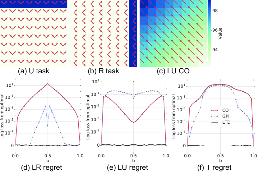
Refer to caption
Figure 5: Additional results for figure 1 (tabular)
(a) The U(p) and (b) R(ight) tasks.
(c) The CO policy for the LU task. Note how even far from the reward (e.g. bottom right corner) the CO policy is near optimal, contrast with the GPI policy for this task (figure 1f).
The log regret (smaller is better) as function of b𝑏b (rb=br1+(1b)r2subscript𝑟𝑏𝑏subscript𝑟11𝑏subscript𝑟2r_{b}=br_{1}+(1-b)r_{2}) for the transfer task for the (d) incompatible (Left-Right) task, (e) compatible (Left Up) task and (f) T(ricky) task.
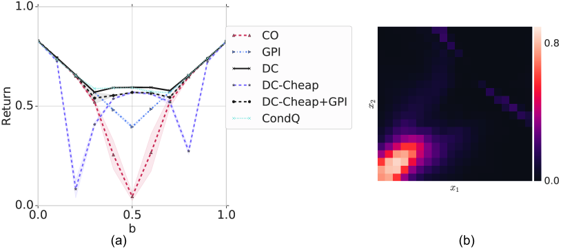
Refer to caption
Figure 6: Additional results for figure 2 (point mass tricky)
(a) The returns (larger is better) for the transfer task as a function of b𝑏b (rb=br1+(1b)r2subscript𝑟𝑏𝑏subscript𝑟11𝑏subscript𝑟2r_{b}=br_{1}+(1-b)r_{2}) including the DC heuristics. DC-Cheap+GPI performs almost as well as DC.
(b) The Rényi divergence of the two base policies as a function of position: the two policies are compatible except near the bottom left corner where the rewards are non-overlapping.
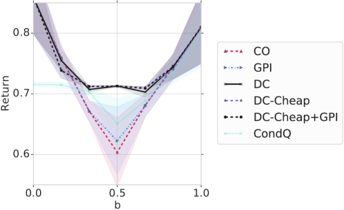
Refer to caption
Figure 7: Returns for figure 3 (planar manipulator)
The returns for the transfer task as a function of b𝑏b (rb=br1+(1b)r2subscript𝑟𝑏𝑏subscript𝑟11𝑏subscript𝑟2r_{b}=br_{1}+(1-b)r_{2}) including the DC heuristics. DC-Cheap+GPI performs almost as well as DC. Shaded bars show SEM (5 seeds).
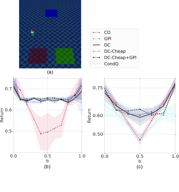
Refer to caption
Figure 8: Additional results for figure 4 (mobile bodies)
(a) Jumping ball task. The task has rewards (1,0),(0,1)1001(1,0),(0,1) in the green and red boxes respectively and (0.75,0.75)0.750.75(0.75,0.75) in the blue square.
The returns for the transfer task as a function of b𝑏b (rb=br1+(1b)r2subscript𝑟𝑏𝑏subscript𝑟11𝑏subscript𝑟2r_{b}=br_{1}+(1-b)r_{2}) including the DC heuristics for the jumping ball (b) and ant (c). Shaded bars show SEM (5 seeds for ant, 3 seeds for jumping ball). As expected, CO performs poorly on these tasks. CondQ struggles to consistently get good returns on the ant task. The DC heuristics perform well on these tasks.
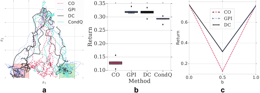
Refer to caption
Figure 9: Ant on non-composable subtasks
(a) Trajectories of the ant during transfer on non-composable subtasks. In this experiment the two base tasks consists of rewards at the red and green square respectively. As expected, in this task, where the two base tasks have no compositional solution, CO (red) performs poorly with trajectories that end up between the two solutions. GPI (blue) performs well, as does DC (black). CondQ does slightly worse.
(b) Box-plot of returns from 5 seeds (at b=0.5𝑏0.5b=0.5).
(c) Returns as a function of b𝑏b, SEM across 5 seeds is plotted, but is smaller than the line thickness.

Appendix F Experiment details

All control tasks were simulated using the MuJoCo physics simulator and constructed using the DM control suite (Tassa et al., 2018) which uses the MuJoCo physics simulator (Todorov et al., 2012).

The point mass was velocity controlled, all other tasks were torque controlled. The planar manipulator task was based off the planar manipulator in the DM control suite. The reward in all tasks was sparse as described in the main text.

During training for all tasks we start states from the randomly sampled positions and orientations. For the point mass, jumping ball and ant we evaluated transfer starting from the center (in the walker environments, the starting orientation was randomly sampled during transfer, the point mass does not have an orientation). For the planar manipulator transfer was tested from same random distribution as in training. Infinite time horizon policies were used for all tasks.

Transfer is made challenging by the need for good exploration. That was not the focus on this work. We aided exploration in several ways: during training we acted according to a higher-temperature policy αe=2αsubscript𝛼𝑒2𝛼\alpha_{e}=2\alpha. We also sampled actions uniformly in an ϵitalic-ϵ\epsilon-greedy fashion with ϵ=0.1italic-ϵ0.1\epsilon=0.1 and added Gaussian exploration noise during training. This was sufficient to explore the state space for most tasks. For the planar manipulator and the jumping ball, we found it necessary to induce behavior tasks by learning tasks for reaching the blue target. This behavior policy was, of course, only used for experience and not during transfer.

Below we list the hyper-parameters and networks use for all experiment. The discount γ𝛾\gamma and α𝛼\alpha were the only sensitive parameters that we needed to vary between tasks to adjust for the differing magnitudes of returns and sensitivity of the action space between bodies. If α𝛼\alpha is too small then the policies often only find one solution and all transfer approaches behave similarly, while for large α𝛼\alpha the resulting policies are too stochastic and do not perform well.

Proposal learning rate 103superscript10310^{-3}
All other learning rates 104superscript10410^{-4}
Value target update period 200200200
Proposal target update period 200200200
𝚼𝚼{\bm{\Upsilon}} target update period 500500500
Number of importance samples for all estimators during learning 200200200
Number of importance samples for acting during training 505050
Number of importance samples for acting during transfer 100010001000
Table 2: Parameters the same across all experiments

The state vector was preprocessed by a linear projection of 3×3\times its dimension and then a tanh\tanh non-linearity. All action-state networks (Q𝑄Q, 𝝍𝝍{\bm{\psi}}, C𝐶C) consisted of 3 hidden layers with elu𝑒𝑙𝑢elu non-linearities (Clevert et al., 2015), with both action and preprocessed state projected by linear layers to be of the same dimensionality and used for input the first layer. All value networks and proposal networks consisted of 2 layers with elu𝑒𝑙𝑢elu non-linearities. The number of neurons in each layer was varied between environments, but was kept the same in all networks and layers (we did not sweep over this parameter, but choose a reasonable number based on our prior on the complexity of the task).

Below we list the per task hyper-parameters

Task Number of units α𝛼\alpha γ𝛾\gamma
Point mass 22 1 0.99
Planar Manipulator 192 0.05 0.99
Jumping Ball 192 0.2 0.9
Ant 252 0.1 0.95
Table 3: Parameters varied between experiments