A blind method to recover the mask of a deep galaxy survey

Abstract

We present a blind method to determine the properties of a foreground contamination, given by a visibility mask, that affects a deep galaxy survey. Angular cross correlations of density fields in different redshift bins are expected to vanish (apart from a contribution due to lensing), but are sensitive to the presence of a foreground that modulates the flux limit across the sky. After formalizing the expected effect of a foreground mask on the measured galaxy density, under a linear, luminosity-dependent bias model for galaxies, we construct two estimators, based on the average or square average galaxy density in a given sky pixel along the line of sight, that single out the mask contribution if a sufficient number of independent redshift bins is available. These estimators are combined to give a reconstruction of the mask. We use Milky-Way reddening as a prototype for the mask. Using a set of 20 large mock catalogs covering $1/4$-th of the sky and number-matched to $H\alpha$ emitters to mimic an Euclid-like sample, we demonstrate that our method can reconstruct the mask and its angular clustering at scales $\ell\,\hbox to0.0pt{\raise 2.15277pt\hbox{$<$}\hss}{\lower 4.30554pt\hbox{$\sim$}}\,100$, beyond which the cosmological signal becomes dominant. The uncertainty of this reconstruction is quantified to be $1/3$-rd of the sample variance of the signal. Such a reconstruction requires knowledge of the average and square average of the mask, but we show that it is possible to recover this information either from external models or internally from the data. It also relies on knowledge of how the impact of the foreground changes with redshift (due to the extinction curve in our case), but this can be tightly constrained by cross correlations of different redshift bins. The strong points of this blind reconstruction technique lies in the ability to find “unknown unknowns” that affect a survey, and in the facility to quantify, using sets of mock catalogs, how its uncertainty propagates to clustering measurements.

1 Introduction

The next generation of galaxy surveys, like Euclid [1], DESI [2], WFIRST [3], LSST [4], eBoss [5] and the SKA [6] surveys, will map large fractions of the sky, going deep, well beyond redshift one, and collecting data for billions of galaxies. They will provide measurements of galaxy clustering to unprecedented sub-percent precision, providing tight constraints to parameters like the equation of state of dark energy and its possible redshift evolution, that may discriminate a pure cosmological constant from a dynamical component. With statistical errors beaten down, the error budget will be dominated by systematics. A class of these systematics is connected with foregrounds on the sky, internal to the Milky Way or related to the nearest galaxies, that modulate the effective depth of the survey. We can broadly divide such foregrounds into those that increase the background noise, like zodiacal light, and those that decrease the signal, like Milky Way extinction. These foregrounds, if not properly corrected for, create large-scale structure on degree scales, that is then projected to the observed redshift to create fake structures at the $\sim$Gpc comoving scales that lie before (in wave number) or at the peak of the galaxy power spectrum.

A very similar effect can be induced by more instrumental issues, like errors in the zero-point calibration of photometry, straylight within the detector, image persistence in the CCD, modulations of survey exposure time or decay of the instrument performance along its lifetime, fiber collision or overlapping spectra in slitless spectroscopy. The impact of these features couples with the survey strategy to determine the effective flux limit of the survey across the sky.

Every team involved in the preparation of the future surveys mentioned above is working hard to model and subtract out these effects. Most of the approaches proposed so far are based either on prior knowledge of the contaminant, or on removal of the most contaminated modes, with some information loss. For instance, removal of contamination due to fiber collision can be done, with some loss of information, by removing purely angular modes in the anisotropic power spectrum [7, 8]. Experience with previous surveys teaches us that real data are often affected by “unknown unknowns”, i.e. sources of contamination that were not accounted for in the preliminary analysis. An example is given by the SDSS-III BOSS survey [9], where stars of the same magnitude as the observed galaxies were decreasing the effective area of the survey, creating spurious power when this decrease was not corrected for. The contamination was found to be strong at scales just beyond the first Baryonic Acoustic Oscillation (BAO), and its cause was found by correlating the galaxy density with a list of potential causes. Correction of systematics in [10, 11] was based on template subtraction, assuming that each potential foreground is contributing linearily to the observed density contrast; the corresponding linear coefficients were found by cross-correlating the signal with the template. This method of template subtraction, coupled with mode deprojection, was further developed by [12, 13]. Besides correlating the observed density with known sources, an often used approach is that of computing cross correlations of very different surveys that are subject to different systematics; in this case it is in principle possible to minimise the contamination. This technique has been used to constrain primordial non-Gaussianities [14, 15, 16]. A caveat to this approach is that the Galaxy is a source of contamination at all wavelengths, so it is not obvious to understand at what level foregrounds at different wavelengths are really uncorrelated. 21 cm intensity mapping analysis exploits the idea that foregrounds are modulated on very different scales, and this makes it possible to perform a blind separation of signal and foreground [17], at the cost of removing large-scale cosmological modes that lie in the same domain as the contaminants. Besides, the analysis of the Cosmic Microwave Background (CMB) can exploit, with component separation techniques, the fact that different components have different Specral Energy Distributions (SEDs) [18], reaching a much higher precision level in foreground subtraction. One could think to extend this principle to galaxy surveys using redshift in place of wavelength: foregrounds could be fitted based on of how their impact on the observed density changes with redshift, see [19, 20] for an example in this direction.

Several foregrounds can be readily subtracted once images are acquired and well calibrated; for instance, the precise origin of the background noise in an image (say zodiacal light, extragalactic background, or straylight) should be known in advance to simulate a survey and assess its completeness, but when images have been taken the noise level is directly measured. The case of Milky Way extinction is different, as the extragalactic light is absorbed by dust grains and reprocessed in the mid and far infrared (FIR), and there is no internal way to know the fraction of absorbed light. Extinction is typically subtracted using models based on observed FIR emission maps of the Galaxy. In Schlegel, Finkbeiner & Davis [21] (hereafter SFD) the authors used COBE and IRAS data to create a map of FIR emission, then transformed this into a reddening map by calibrating it with reddening values measured for a set of galaxies. More recently, the Planck Collaboration issued two extinction or reddening maps, based on the same principles. The first map was issued with the 2013 results [22] (hereafter P13): they used 353, 545 and 857 GHz maps, together with IRAS 100 $\mu$m map, and fitted the SED of each pixel with a modified black body. They then used the radiance as a quantity supposedly well correlated with extinction, and calibrated the coefficient of this linear correlation with reddening measured for a set of 53,399 SDSS quasars. Care was taken in minimizing the impact of Cosmic Infrared Background (CIB) fluctuations on reddening estimates. In 2015 a different map was issued, based on Planck intermediate results [23] (hereafter P15): they added to the previous maps the IRAS 60 $\mu$m and the WISE 12 $\mu$m bands, and fitted pixel-by-pixel SEDS with a physical dust model by Draine & Li [24], where extinction $A_{V}$ is a parameter of the model. However, a check with 272,366 SDSS quasars showed that extinction was overestimated by a factor of 2.4, so the extinction maps were corrected by that heuristic factor. We will show in this paper that the level of agreement of these three reddening or extinction maps is insufficient to guarantee the required accuracy in foreground subtraction.

These foregrounds are expected to be dominant at very large scales. In fact, at scales beyond the peak of the power spectrum the clustering signal is expected to be weak, while foregrounds, being driven by local astrophysical entities that surround the Earth, are clustered on very large angular scales; the same is true for instrumental and survey issues (with remarkable exceptions of fiber collision or spectra overlap that will be discussed in the conclusions). While their impact at the very important BAO scales is typically under control, measuring clustering at the largest scales will be limited by foreground subtraction. There are several science cases that require accurate measurements at the largest scale. In the standard scenario, these scales have been frozen once they exited the Hubble horizon during the inflationary epoch, and they are the neatest fossil to understand the physical interactions at the inflationary energy scale. These interactions may have generated some primordial non-gaussianity, whose amplitude is usually parametrized by $f_{\rm nl}$. Planck has constrained this parameter to be $f_{\rm nl}=0.8\pm 5.0$ [25]. While the search of generic primordial non-gaussianity requires an analysis beyond the 2-point statistics, local non-gaussianity generates a well-defined scale-dependent galaxy bias [26] which is enhanced on large scales. This can be exploited to achieve tighter constraints than Planck’s, especially using multiple tracers [27] in future redshift surveys. Moreover, at the largest scales the simple Newtonian approximation may start to fail; in the last decade several efforts have been devoted to describing galaxy clustering in a gauge-invariant relativistic framework [28, 29, 30] to meet the experimental accuracy of coming surveys. These effects are expected to be relevant at the horizon scale and their amplitude and detectability are comparable with $f_{\rm nl}\sim\mathscr{O}(1)$ [31].

Proper subtraction of foregrounds is only part of the problem, the uncertainty on foreground removal should be quantified in terms of its contribution to the covariance matrix of clustering measurements, and propagated to parameter estimation. In a recent paper, Colavincenzo et al. [32] (hereafter C17), the authors quantified, with an idealized foreground model, the impact of the uncertainty of foreground subtraction on the covariance matrix of the power spectrum of dark matter halos, showing that, although cosmological clustering and foreground are assumed to be uncorrelated, the full covariance matrix is not simply the sum of the cosmological one and that induced by the foreground, because of a rather long list of mixed terms that can be quite significant.

To determine the full covariance matrix it is necessary to know not only the error on foreground subtraction but also its correlations on the sky. Foregrounds mainly impact clustering measurements through a modulation of survey depth. We will loosely call “visibility mask”, or simply “mask”, a function of the sky position $\bm{\theta}$ that is responsible for the modulation of survey depth, though its specific impact may in general depend on the target redshift. Throughout the paper we will use galactic extinction (more specifically, $E(B-V)$ reddening) as a prototype mask. The starting idea is that (see e.g. C17) to first order a foreground mask ${\cal M}$ acts on the survey in such a way that the observed density contrast $\delta_{\rm o}$ is related to the true galaxy density contrast $\delta_{\rm g}$ as $1+\delta_{\rm o}=(1-{\cal M})(1+\delta_{\rm g})$ (see equation (2.19) of C17). The two-point correlation function of the density is then:

$$\langle\delta_{\rm o1}\delta_{\rm o2}\rangle=\langle\delta_{\rm g1}\delta_{\rm g2}\rangle+\langle{\cal M}_{1}{\cal M}_{2}\rangle+\langle\delta_{\rm g1}\delta_{\rm g2}\rangle\langle{\cal M}_{1}{\cal M}_{2}\rangle\,.$$ (1.1)

Then, if we measure a cosmic correlation that is expected to be vanishing, $\langle\delta_{\rm g1}\delta_{\rm g2}\rangle=0$, like the angular cross-correlation of two different and distant redshift bins, any significant signal could be interpreted as the angular correlation of the foreground, and used to reconstruct it. This will provide accurate results as long as the survey is deep enough to have a large number of independent pairs of redshift bins.

In this paper we build on this idea, presenting a blind method to recover the mask to which a cosmological catalog is subject. The method will be applied to a set of mock galaxy catalogs on the past light cone covering $1/4$ of the sky, generated with the PINOCCHIO approximate method [33, 34], and calibrated to generate an Euclid-like survey of $H\alpha$ emitters [35] in a wide redshift range. The reconstruction of the mask will be based on estimators of the average density contrast along the line of sight; the inversion of the relation between mask and estimator requires knowledge of the first two moments of the mask, and we will show how this information can be achieved with sufficient accuracy from an internal analysis of the catalog. We will check that the cross correlation induced by light-cone effects, like magnification bias due to lensing, does not affect the scale where our prototypical mask is dominant and can be recovered. We will further show to what level this reconstruction can be used to test different maps of galactic extinction, in the case this is the only present foreground.

The paper is organized as follows. Section 2 gives a formalization of the problem, defining the observed density contrast and its dependence on the flux limit of the survey, and expanding the equations in the case of galactic extinction as foreground. Section 3 describes the simulated catalogs of dark matter halos in the past light-cone and the abundance-matching connection of halos with galaxies. Section 4 describes the procedure adopted to obtain a “best reconstruction” for the mask, starting from estimators of galaxy clustering that are sensitive only to the mask term, and under the hypothesis that the first two moments of the mask are known. Section 5 discusses how the angular clustering of the cosmological, unmasked mocks can be recovered using the mask best reconstruction, and the crucial role of cross correlations for the calibration of the mask. Section 6 discusses how the first two moments of the mask can be estimated from the available data, and tests the performance of a best reconstruction applied with no external information and calibrated on cross-correlations. Section 7 shows to what extent an application of this procedure can be used to test reddening maps and recover the extinction curve. Section 8 presents a final discussion and the conclusions.

2 The impact of a visibility mask on clustering measurements

2.1 The galaxy density contrast

A density measurement is based on counting galaxies that are observed in specified volumes. The condition for a galaxy to be observed is typically expressed as a flux limit threshold. In realistic cases, the probability of a galaxy being observed will be a smooth function of flux; this will be quantified by a completeness function, obtained through detailed simulations of the observational setup. Knowledge of the completeness function allows one to recast the observational condition into a strict flux limit threshold, that at a certain redshift $z$ can be recast into a luminosity threshold $L_{0}(z)$ by assuming a fiducial cosmology.

We call $\Phi(L|z)$ the galaxy luminosity function at redshift $z$, and $\phi_{\rm local}(L|\mathbf{x})$ the local luminosity function in a volume centred on the comoving position $\mathbf{x}$, lying at the redshift $z$: $|\mathbf{x}|=d_{c}(z)$, where $d_{c}(z)$ is the comoving distance from the observer. The relation between $\Phi$ and $\phi_{\rm local}$ is given by an average over the shell of the survey volume within a redshift bin $\Delta z$ around $z$. We denote such an average by $\langle\cdots\rangle$, so that:

$$\Phi(L|z)=\langle\phi_{\rm local}(L|{\mathbf{x}})\rangle\,.$$ (2.1)

We stress that $\langle\cdots\rangle$ does not denote an ensemble average in this paper. The integrals in luminosity, from $L_{0}$ to $\infty$, of $\phi_{\rm local}$ and $\Phi$ give, respectively, the local galaxy density $n_{g}(\mathbf{x}|L_{0})$ and the average galaxy density $\langle n_{\rm g}\rangle(z|L_{0})$:

$$n_{g}(\mathbf{x}|L_{0})=\int_{L_{0}(z)}^{\infty}\phi_{\rm local}(L|{\mathbf{x}})dL\,,\ \ \ \ \ \ \ \ \ \langle n_{\rm g}\rangle(z|L_{0})=\int_{L_{0}(z)}^{\infty}\Phi(L|z)dL\,.$$ (2.2)

Under the assumption that the shape of the luminosity function is independent of environment, $\phi_{\rm local}(L|\mathbf{x})$ differs from $\Phi(L|z)$ only in the normalization:

$$\phi_{\rm local}(L|\mathbf{x})=[1+\delta_{\phi}(\mathbf{x})]\Phi(L|z)\,.$$ (2.3)

We define the galaxy density contrast in the usual way:

$$\delta_{\rm g}=\frac{n_{g}-\langle n_{\rm g}\rangle}{\langle n_{\rm g}\rangle}\,.$$ (2.4)

We are using here two different symbols for $\delta_{\phi}$ and $\delta_{\rm g}$ because the two quantities have a different relation with the underlying matter density contrast, due to the fact that galaxy bias in general depends on galaxy luminosity. We will restrict ourself here to a simple linear, luminosity-dependent bias model to relate the galaxy density contrast $\delta_{\rm g}$ to the matter density contrast $\delta$ in the same volume used to count galaxies:

$$\delta_{\rm g}(\mathbf{x}|L_{0})=b_{1}(L_{0},z)\delta(\mathbf{x})\,,\ \ \ \ \ \ \ \ \ \delta_{\phi}(\mathbf{x}|L)=\beta_{1}(L,z)\delta(\mathbf{x})$$ (2.5)

where $b_{1}(L_{0},z)$ is the galaxy linear bias and

$$b_{1}(L_{0},z)=\frac{1}{\langle n_{\rm g}(z|L_{0})\rangle}\int_{L_{0}(z)}^{\infty}\beta_{1}(L,z)\Phi(L|z)dL\,.$$ (2.6)

Getting back to equation 2.3, we note that a luminosity-dependent bias implies that $\delta_{\phi}$ gets a dependence on luminosity (equation 2.5), and so the shape of the local luminosity function is not strictly universal. We will neglect this second-order effect in this paper.

2.2 Observed density contrast in presence of a foreground

A foreground contamination will have the effect of modulating the flux limit on the sky. We denote here the sky position with the two-dimensional vector $\bm{\theta}$; this is related to the comoving position $\mathbf{x}$ as its angular part in a spherical coordinate system, the radius $r=|\mathbf{x}|$ being given by $d_{c}(z)$. We call $L_{\rm lim}(\bm{\theta},z)$ the flux limit in a given angular position $\bm{\theta}$ of the sky, pointing to the position $\mathbf{x}$. In the following, we will not explicitly write the $z$-dependence of the various quantities. The observed number density will thus be:

$$n_{\rm o}(\mathbf{x})=\int_{L_{\rm lim}(\bm{\theta})}^{\infty}\phi_{\rm local}(L|\mathbf{x})dL\,.$$ (2.7)

We can write the luminosity threshold as:

$$L_{\rm lim}(\bm{\theta})=L_{0}+\delta L(\bm{\theta})\,.$$ (2.8)

In general, the perturbation $\delta L(\bm{\theta})$ will not average to zero over the survey. This is easy to see in the case of galactic extinction: $L_{0}$ will be the luminosity limit without extinction, and $\delta L$ will always be positive, as extinction acts in increasing the limiting flux and luminosity.

For small perturbations of the luminosity threshold $\delta L$, one can Taylor-expand the observed density. It is convenient to define the quantity

$$\epsilon\equiv\delta L/L_{0}$$ (2.9)

and two redshift-dependent scaling functions related to the luminosity function and its $L$-derivative:

$$S_{A}(z)\equiv\frac{\langle n_{\rm g}\rangle(z)}{\Phi(L_{0}|z)L_{0}(z)}\,,$$ (2.10)

$$S_{B}(z)\equiv\frac{d\Phi}{dL}(L_{0}|z)\frac{L_{0}(z)}{2\Phi(L_{0}|z)}+\frac{1}{2}\,.$$ (2.11)

Both scaling functions depend only on the shape of the luminosity function beyond or at $L_{0}$. The convenience of adding $1/2$ to $S_{B}$ will be clear later. It is worth noticing that $2S_{B}-1=d\ln\Phi/d\ln L$ evaluated at $L=L_{0}$, and if $\Phi$ is modeled as a Schechter function with slope $\alpha$ (including its negative sign) and characteristic luminosity $L_{\star}$, then $S_{B}=(\alpha-L_{0}/L_{\star}+1)/2$.

The observed density can be thus written as:

$$\frac{n_{\rm o}}{\Phi L_{0}}=\frac{n_{\rm g}}{\Phi L_{0}}-(1+\beta_{1}\delta)\,\epsilon-\left(S_{B}-\frac{1}{2}\,\right)\left[1+\left(\beta_{1}+\beta_{1}^{\prime}\frac{\Phi}{\Phi^{\prime}}\right)\delta\right]\,\epsilon^{2}+O(\epsilon^{3})\,.$$ (2.12)

It is convenient to note that $n_{\rm g}/\Phi L_{0}=S_{A}(1+b_{1}\delta)$. In this equation the prime denotes a derivative with respect to $L$, and again all $L$-dependent functions are evaluated at $L_{0}$.

To compute $\langle n_{\rm o}\rangle$ we can assume no correlation between $\delta L(\bm{\theta})$ (and thus $\epsilon(\bm{\theta})$) and $\delta(\mathbf{x})$. This is true, in an ensemble-average sense, whenever the foreground is independent of the cosmological signal. This covers most foregrounds, with some remarkable exceptions, the obvious cases being density-dependent biases like fiber collision or spectra overlapping in slitless spectroscopy. Moreover, a reddening map obtained from FIR observations will be contaminated by the Cosmic Infrared Background, that gets a contribution by the same surveyed galaxies (see discussion in [22]), so if extinction is corrected for using such a map the residual foreground will be correlated with the cosmological signal; we will further discuss this point in Section 8. We should notice, however, that even in the case of no correlation between $\epsilon$ and $\delta$, a given volume average does not guarantee that terms like $\langle\epsilon\delta\rangle$ go to zero exactly. We do not attempt here an estimation of the magnitude of these residual terms. Their impact will be implicitely taken into account when we will quantify the accuracy of our method using simulations. Neglecting cross terms of mask and cosmological signal, the average observed density is:

$$\frac{\langle n_{\rm o}\rangle}{\Phi L_{0}}=S_{A}-\langle\epsilon\rangle-\left(S_{B}-\frac{1}{2}\,\right)\langle\epsilon^{2}\rangle+O(\epsilon^{3})\,,$$ (2.13)

so that the average density is affected by the foreground already at first order in $\epsilon$ if the perturbation does not average to zero. The second-order effect is due to the curvature of the luminosity function at the luminosity threshold, that gives an imbalance between galaxies that get in or out of the selection.

The resulting galaxy density contrast can be written as the sum of a cosmological ($T_{\rm c}\delta$) and a non-cosmological ($T_{\rm nc}$) term:

$$\delta_{\rm o} = \frac{n_{\rm o}-\langle n_{\rm o}\rangle}{\langle n_{\rm o}\rangle}=T_{\rm nc}+T_{\rm c}\,\delta\,,$$ (2.14)

$$T_{\rm nc} = -\frac{1}{S_{A}}(\epsilon-\langle\epsilon\rangle)-\frac{1}{S_{A}^{2}}\langle\epsilon\rangle(\epsilon-\langle\epsilon\rangle)-\frac{S_{B}-\frac{1}{2}}{S_{A}}(\epsilon^{2}-\langle\epsilon^{2}\rangle)+O(\epsilon^{3})\,,$$

$$T_{\rm c} = b_{1}-\frac{\beta_{1}\epsilon-b_{1}\langle\epsilon\rangle}{S_{A}}-\frac{\left(S_{B}-\frac{1}{2}\right)\left(\beta_{1}+\beta_{1}^{\prime}\frac{\Phi}{\Phi^{\prime}}\right)}{S_{A}}\,\epsilon^{2}$$

$$-\frac{\beta_{1}}{S_{A}^{2}}\,\langle\epsilon\rangle\,\epsilon+\frac{1+S_{A}\left(S_{B}-\frac{1}{2}\right)}{S_{A}^{2}}b_{1}\langle\epsilon^{2}\rangle+O(\epsilon^{3})\,.$$

If no foreground is present then $\epsilon=0$ and the non-cosmological term $T_{\rm nc}$ vanishes as expected. We will consider later a (toy-model) case where bias is independent of luminosity; in this case $b_{1}=\beta_{1}$ and $\beta_{1}^{\prime}=0$, and equation 2.2 can be simplified to take the form compatible with equation 2.19 of C17 and with the form assumed to obtain equation 1.1:

$$1+\delta_{\rm o}=(1-A)(1+\delta_{\rm g})\,,$$ (2.15)

where

$$A=\frac{1}{S_{A}}(\epsilon-\langle\epsilon\rangle)+\frac{1}{S_{A}^{2}}\langle\epsilon\rangle(\epsilon-\langle\epsilon\rangle)+\frac{S_{B}-\frac{1}{2}}{S_{A}}(\epsilon^{2}-\langle\epsilon^{2}\rangle)+O(\epsilon^{3})\,.$$ (2.16)

In this case $T_{\rm nc}=-A$ and $T_{\rm c}=1-A$.

2.3 Milky Way extinction

As a prototype of foreground contamination that modulates survey depth $\delta L(\bm{\theta})$, we choose Milky Way extinction. Extinction at a wavelength $\lambda$, quantified as a magnitude, is denoted as $A_{\lambda}=R(\lambda)E(B-V)$, where $E(B-V)$ is the reddening and $R(\lambda)$ an extinction curve. Reddening only depends on the sky position, so we define the “visibility mask” ${\cal M}(\bm{\theta}):=E(B-V)$ as the reddening. We will assume (see next section) that our Euclid-like catalogs consist of galaxies that are detected in $H\alpha$ emission, so the impact of extinction on galaxy selection acquires a redshift dependence. The luminosity limit of the survey is:

$$L_{\rm lim}(\bm{\theta},z)=L_{0}10^{0.4R(z){\mathscr{M}}(\bm{\theta})}\,,$$ (2.17)

where $R(\lambda)$ is computed at the wavelength of the $H\alpha$ line at redshift $z$, $6563\times(1+z)$ Å. It is useful to define the scaling function:

$$S_{C}(z)=0.4\ln 10\,R(z)\,.$$ (2.18)

Extragalactic surveys usually observe sky areas with $E(B-V)\,\hbox to0.0pt{\raise 2.15277pt\hbox{$<$}\hss}{\lower 4.30554pt\hbox{$\sim$}}\,0.1$, so, for a typical extinction curve, the largest values of $S_{C}{\cal M}$ will range from $\sim 0.2$ in the $R$ band ($z\sim 0$) to $\sim 0.03$ in the $K$ band ($z\sim 2.4$). The relative variation of flux limit $\epsilon$ is then worked out to second order as:

$$\epsilon(\bm{\theta},z)={\rm e}^{S_{C}(z)\,{\cal M}(\bm{\theta})}-1=S_{C}(z){\cal M}(\bm{\theta})+\frac{1}{2}S_{C}^{2}(z){\cal M}^{2}(\bm{\theta})+O({\cal M}^{3})\,,$$ (2.19)

The observed density contrast is thus expressed as:

$$\delta_{\rm o} = T_{\rm nc}+T_{\rm c}\,\delta\,,$$ (2.20)

$$T_{\rm nc} = -\frac{S_{C}}{S_{A}}({\cal M}-\langle{\cal M}\rangle)-\frac{S_{C}^{2}}{S_{A}^{2}}\langle{\cal M}\rangle({\cal M}-\langle{\cal M}\rangle)-\frac{S_{B}S_{C}^{2}}{S_{A}}({\cal M}^{2}-\langle{\cal M}^{2}\rangle)+O({\cal M}^{3})\,,$$

$$T_{\rm c} = b_{1}-\frac{S_{C}}{S_{A}}(\beta_{1}{\cal M}-b_{1}\langle{\cal M}\rangle)-\frac{S_{B}S_{C}^{2}}{S_{A}}(\beta_{1}{\cal M}^{2}-b_{1}\langle{\cal M}^{2}\rangle)-\frac{S_{C}^{2}}{S_{A}^{2}}\beta_{1}{\cal M}\langle{\cal M}\rangle$$

$$-\frac{\left(S_{B}-\frac{1}{2}\right)S_{C}^{2}}{S_{A}}\beta_{1}^{\prime}\frac{\Phi}{\Phi^{\prime}}{\cal M}^{2}+\frac{S_{C}^{2}}{S_{A}^{2}}b_{1}\langle{\cal M}^{2}\rangle+O({\cal M}^{3})\,.$$

For a bias that is independent of luminosity:

$$1+\delta_{\rm o}=(1-A)(1+\delta_{\rm g})\,,\,$$ (2.21)

with

$$A=\frac{S_{C}}{S_{A}}({\cal M}-\langle{\cal M}\rangle)+\frac{S_{C}^{2}}{S_{A}^{2}}\langle{\cal M}\rangle({\cal M}-\langle{\cal M}\rangle)+\frac{S_{B}S_{C}^{2}}{S_{A}}({\cal M}^{2}-\langle{\cal M}^{2}\rangle)+O({\cal M}^{3})\,.$$ (2.22)

This clarifies the reason why we added $1/2$ to the definition of $S_{B}$ in equation 2.11: it was done to get here a more compact form for $T_{\rm nc}$. It is worth noticing here that the three functions $S_{A}$, $S_{B}$ and $S_{C}$ for a survey can be computed from the galaxy luminosity function and from the extinction curve, and so it is possible to assume them as known functions. We will discuss the role of the extinction curve in Section 7.

It is important to stress the domain of validity of equation 2.20: we have assumed no correlation between $\epsilon(\bm{\theta})$ and $\delta({\mathbf{x}})$ and we have neglected residual correlations due to the fact that volume averages are not ensemble averages; we have assumed no environmental dependence of the shape of the luminosity function, a linear bias scheme and a second-order expansion of the integral and of the exponential that relates $\epsilon$ and ${\cal M}$. Next step, carried out in Section 4.1, is to construct estimators that can average out the cosmological term $T_{\rm c}\delta$ and single out the mask-dependent term $T_{\rm nc}$ in that equation.

Real surveys will be affected by several foregrounds at the same time, so what one would measure is their combined effect. However, the way different foregrounds impact as a function of redshift, i.e. their $S_{C}(z)$ functions, may be different. For instance, a photometric selection based on a single apparent magnitude, or a wavelength-independent modulation of the photometric zero-point, would give a constant $S_{C}$ function. The present method should then be generalized to a sum of contributions, grouped according to the shape of their $S_{C}(z)$ functions. For sake of simplicity we will not consider this extension in this paper.

3 Simulated catalogs

To build and test our method, we generated a set of 20 large simulated catalogs of dark matter halos on the observer past light cone. The catalogs were generated with the PINOCCHIO approximate method [33, 34]; see [36] for a review on this technique.

PINOCCHIO is a parallel code that implements the following semi-analytic scheme: starting from a linear density contrast field sampled on a regular cubic grid (as in the construction of initial conditions for an N-body simulation), it predicts, for each grid element (or particle), the time at which it is expected to collapse (to suffer orbit crossing). This is done by smoothing the linear density contrast on a set of scales, computing the collapse time using ellipsoidal collapse as in [37], and then taking for each particle the earliest obtained collapse time. Collapsed particles are then grouped into halos with an algorithm that mimics their hierarchical assembly. Halo positions are computing using 3rd-order Lagrangian Perturbation Theory [38, 39, 40].

With the latest version of the code, we run 20 independent realizations of a box of 3.2 Gpc$/h$, sampled with $4096^{3}$ particles. We used a WMAP cosmology with $\Omega_{0}=0.285$, $\Omega_{\Lambda}=0.715$, $\Omega_{b}=0.044$, $h=0.695$, $\sigma_{8}=0.828$, $n_{s}=0.9632$. Each particle has a mass of $3.77\times 10^{10}\ {\rm M}_{\odot}/h$ and, as we identified halos of at least 20 particles, the smallest resolved halo has mass $7.54\times 10^{11}\ {\rm M}_{\odot}/h$. Halos were output on the past light cone, from $z=2.5$ to $z=0$, on a comoving volume given by the projection of a sky circular area with semi-aperture of $60^{\circ}$, thus covering $1/4$ of the sky. The box was replicated using periodic boundary conditions to fill the cone volume.

We produced a sample of mock galaxy catalogs that broadly mimic the spectroscopic survey of the forthcoming Euclid satellite. This will observe star-forming galaxies through slit-less spectroscopy over disconnected regions covering $\sim 1/3$ of the sky (separated by the Milky Way and the ecliptic). Such galaxies will mainly be detected through their $H\alpha$ emission line (blended with $[NII]$), in a redshift range that has been revised (with respect to the initial red book [1] assumption) to be from 0.9 to 1.75. We will make use of a larger redshift range, in order to have a larger number of independent redshift bins. Indeed, the amount of information available to reconstruct the mask will not be limited to this spectroscopic sample, it will be possible to apply the same technique to the photometric sample, to more distant emission line galaxies (e.g. Lyman-$\alpha$ emitters) and to quasars, thus justyfing the first tests of the method on a larger redshift range. This point will be further discussed in the conclusions.

Assuming a one-to-one relation between halo mass and galaxy luminosity in the $H\alpha$ line (as in a naive Halo Occupation Distribution model - HOD - with one single galaxy in each halo), halos were number-matched to galaxies using the luminosity function of model 1 of Pozzetti et al. (2016) [35]. This was done by dividing the redshift range from 0 to 2.5 in bins of width $\delta z=0.05$; for each bin the cumulative mass function of halos was computed by averaging over the 20 light cones. Since halo masses take discrete values multiples of the particle mass, we redefine halo masses by assuming that a halo of $N_{p}$ particles of mass $M_{p}$ has a mass distributed in the interval from $N_{p}M_{p}$ to $(N_{p}+1)M_{p}$, with a mass function equal to a power-law interpolation of the numerical halo mass function at the same mass and redshift bin. The relation between halo mass $M$ and $H\alpha$ luminosity $L$ was then found by tracking at which $M$ and $L$ values the cumulative mass and luminosity functions give the same number density. The matching luminosities were interpolated with polynomials in mass and redshift, to construct a function that assigns a luminosity to each halo. This interpolation induces very little differences in the luminosity function at a redshift around $z=1.3$, where the $\Phi_{\star}$ parameter of the Schechter fit in model 1 of Pozzetti has a break. These differences are far smaller than the $\sim 0.2$ uncertainty in the number density of $H\alpha$ galaxies.

With this naive HOD model we obtained 20 mock galaxy catalogs covering $1/4$ of the sky, with known angular position, observed redshift (including redshift-space distortions) and $H\alpha$ luminosity matching model 1 of Pozzetti. We assumed that the redshift is known without observational uncertainty. Mock galaxy samples were selected using a flux limit of $2\times 10^{-16}\ {\rm erg\ s}^{-1}\ {\rm cm}^{-2}$. As a matter of fact, the halo mass limit of 20 particles sets a redshift-dependent luminosity completeness, that may be higher than the luminosity corresponding to the flux limit; in this case the sample is incomplete and this happens at $z<0.75$, so we will consider in this paper the redshift range from $z=0.8$ to $z=2.4$. One obvious problem of these mock catalogs is that, assuming a one-to-one relation between halos and galaxies, the 1-halo term that dominates clustering on small scales is completely missing. Because we are mostly focused on very large scales, this issue is not a worry in this context.

Due to the luminosity dependence of (linear) bias, the $T_{\rm c}$ term in equation 2.20 for the observed density contrast is complicated by the presence of three bias terms $b_{1}$, $\beta_{1}$ and $\beta_{1}^{\prime}$. These do not enter in the reconstruction of the visibility mask, that is based on $T_{\rm nc}$ in the same equation, so their relevance is limited. However they introduce a further level of complication in the analysis, that is convenient to avoid at this stage. We decided to remove the luminosity dependence of bias with the following procedure: for each redshift bin used in the abundance matching procedure, we shuffle the values of halo masses, and $H\alpha$ luminosities, among all the halos. The halo mass function is unchanged, and so is the abundance matching procedure. This way, a selection in luminosity will imply a random sampling of the halos, so the selected sample will have the same linear bias $b_{1}$ independent of luminosity. As a consequence, equation 2.21 will apply in place of equation 2.20. We however warn the reader that bias generally depends on luminosity, so these mock catalogs can be considered only as a convenient toy model of galaxy clustering.

For the mask, we considered the three extinction maps described above, SFD, P13 and P15. All maps are provided to the community as HEALPIX maps of either $E(B-V)$ reddening (SFD and P13) or $A_{V}$ extinction. SFD is provided in a pixelization with NSIDE=512 while Planck maps are characterised by the higher resolution of NSIDE=2048. As large scales are of interest here, we resampled Planck maps to NSIDE=512 and used $R_{V}=3.1$ to relate reddening and extinction: $A_{V}=3.1E(B-V)$. We will use P13 as our reference visibility mask: ${\cal M}_{\rm true}={\cal M}_{\rm P13}=E(B-V)_{\rm P13}$. For the extinction curve $R(\lambda)$ we adopted the determination of [41]. To avoid the plane of the Milky Way the axis of the light cone was oriented toward the north galactic pole. Mocks were masked by imposing a different limiting flux in each healpix sky cell. Galaxy catalogs are divided into $N_{z}=17$ redshift bins, centered around $z_{i}=0.8+i\Delta z$, with $i$ ranging from 0 to $N_{z}-1$ and $\Delta z=0.1$, twice the value used for abundance matching. The total redshift range is thus limited to $0.75<z<2.45$. Maps of galaxy density contrast $\delta_{\rm o}$ were computed, for each redshift bin, by counting galaxies in each (equal area) sky pixel covered by our survey, using the same NSIDE=512 healpix map used for the mask, then dividing the counts by the mean number of galaxies per pixel and subtracting $1$. This was done for both the unmasked and the masked versions of the catalogs.

Figure 1: Scaling functions $S_{A}(z)$, $S_{B}(z)$ and $S_{C}(z)$ for our sample selection, and linear galaxy bias $b_{1}(z)$, computed for halos with mass $M\geq 20M_{p}$.

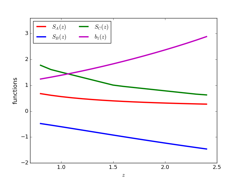
Figure 1 shows the three scaling functions, $S_{A}(z)$, $S_{B}(z)$ and $S_{C}(z)$, computed for our catalog selection, based on the assumed luminosity function and extinction curve. The figure shows also the value of the linear bias $b_{1}(z)$, measured at a set of redshifts (where outputs for the whole periodic simulation box were available) by comparing the halo power spectrum, measured with the code of [42], with the linear power spectrum; values at other redshifts are obtained by interpolation. This bias is computed for all the halos with $M\geq 20M_{p}$, so it applies to the catalogs obtained with shuffled halo masses and is independent of luminosity.

4 Reconstruction of the visibility mask

4.1 Estimators of the mask-dependent term in the observed density contrast

The non-cosmological term $T_{\rm nc}$ of equation 2.20 depends only on the visibility mask, and can be singled out by averaging, pixel by pixel, the observed density measurement $\delta_{\rm o}$ over several redshift bins, under the assumption that the cosmic density contrast $\delta$ averages to zero, at least in an ensemble-average sense, along the same line of sight. This averaging will be imperfect because it will be carried out over a limited volume (and with redshift-dependent weights given by $T_{\rm c}$), and not over a large number of realizations; in this paper we will carefully quantify this residual by applying the method to our set of mock catalogs.

In $T_{\rm nc}$ the mask appears through the terms $\langle{\cal M}\rangle$, $({\cal M}-\langle{\cal M}\rangle)$ and $({\cal M}^{2}-\langle{\cal M}^{2}\rangle)$. The inversion of this relation is affected by multiple solutions at low mask values, the most interesting regions for an extragalactic survey. However, prior knowledge of the first two moments of the mask, $\langle{\cal M}\rangle$ and $\langle{\cal M}^{2}\rangle$, allows to recast the problem in a more convenient way. In the following we will assume that $\langle{\cal M}\rangle$ and $\langle{\cal M}^{2}\rangle$ are known, we will demonstrate in Section 6 that these moments can be worked out to a sufficient accuracy, either by using external data or by internally estimating them from the galaxy survey.

With prior knowledge of the first two moments of the mask, it is possible, using equation 2.13, to recover the true average galaxy density $\langle n_{\rm g}\rangle$ from the observed $\langle n_{\rm o}\rangle$ and from the $S_{B}$ and $S_{C}$ scaling functions:

$$\frac{\langle n_{\rm g}\rangle}{\Phi L_{0}}=\frac{\langle n_{\rm o}\rangle}{\Phi L_{0}}+S_{C}(z)\langle{\cal M}\rangle+S_{B}(z)S_{C}(z)^{2}\langle{\cal M}^{2}\rangle\,.$$ (4.1)

It is useful to define a rescaled density contrast $\delta_{\rm r}$ as:

$$\delta_{\rm r}:=\frac{n_{\rm o}}{\langle n_{\rm g}\rangle}-1=T_{\rm nc}+T_{\rm c}\,\delta=-\left[\frac{S_{C}}{S_{A}}{\cal M}+\frac{S_{B}S_{C}^{2}}{S_{A}}{\cal M}^{2}\right]\\ +\left[b_{1}-\frac{S_{C}}{S_{A}}\beta_{1}{\cal M}-\frac{S_{B}S_{C}^{2}}{S_{A}}\beta_{1}{\cal M}^{2}+\frac{\left(S_{B}-\frac{1}{2}\,\right)S_{C}^{2}}{S_{A}}\beta_{1}^{\prime}\frac{\Phi}{\Phi^{\prime}}{\cal M}^{2}\right]\times\delta+O({\cal M}^{3})\,.$$ (4.2)

When bias is independent of luminosity:

$$1+\delta_{\rm r}=(1-A)(1+\delta_{\rm g})\,,\ \ \ \ \ \ \ \ \ \ A=\frac{S_{C}}{S_{A}}{\cal M}+\frac{S_{B}S_{C}^{2}}{S_{A}}{\cal M}^{2}\,.$$ (4.3)

In what follows we denote the values of the $S_{A}$, $S_{B}$ and $S_{C}$ functions, evaluated at the central redshift $z_{i}$ of the $i-$th bin, as $S_{Ai}=S_{A}(z_{i})$, $S_{Bi}=S_{B}(z_{i})$ and $S_{Ci}=S_{C}(z_{i})$. We define two estimators that average out, in an ensemble average sense, the cosmological signal and single out the redshift average of $T_{\rm nc}$ term, that depends only on the mask ${\cal M}$. The average density estimator $E_{\rm av}(\bm{\theta})$ in each sky pixel is defined as:

$$E_{\rm av}(\bm{\theta})\equiv\frac{1}{N_{z}}\sum_{i}\delta_{\rm r}([z_{i},\bm{\theta}])\simeq-\frac{1}{N_{z}}\sum_{i}\frac{S_{Ci}}{S_{Ai}}{\cal M}-\frac{1}{N_{z}}\sum_{i}\frac{S_{Bi}S_{Ci}^{2}}{S_{Ai}}{\cal M}^{2}+O({\cal M}^{3})\,.$$ (4.4)

The sum is over all $N_{z}$ redshift bins; here we have made it explicit that the position $\mathbf{x}$ is decomposed into angular and redshift coordinates: $\mathbf{x}=[z_{i},\bm{\theta}]$. The square average density estimator $E_{\rm sq}(\bm{\theta})$ is defined as:

$$E_{\rm sq}(\bm{\theta})\equiv\frac{1}{N_{p}}\sum_{i}\sum_{j>i}\delta_{\rm r}([z_{i},\bm{\theta}])\delta_{\rm r}([z_{j},\bm{\theta}])\\ \simeq\frac{1}{N_{p}}\sum_{i}\sum_{j>i}\frac{S_{Ci}S_{Cj}}{S_{Ai}S_{Aj}}{\cal M}^{2}+\frac{1}{N_{p}}\sum_{i}\sum_{j>i}\frac{S_{Ci}S_{Cj}(S_{Bi}S_{Ci}+S_{Bj}S_{Cj})}{S_{Ai}S_{Aj}}{\cal M}^{3}+O({\cal M}^{4})\,.$$ (4.5)

Here $N_{p}=N_{z}(N_{z}-1)/2$ is the number of independent pairs of redshift bins, considering each pair only once; for $N_{z}=17$ we have $N_{p}=136$. The sum in equation 4.5 could be limited by removing nearby redshift bin pairs, that may be affected by residual cosmological correlation. We will show in Section 5.3 that this correlation is marginal, in the following we keep all redshift bin pairs to maximize the signal.

The quadratic and cubic algebraic equations 4.4 and 4.5 can be inverted to provide, for each pixel, estimates of the mask term that we will call ${\cal M}_{\rm av}$ and ${\cal M}_{\rm sq}$. It is important to notice that the two mask reconstructions are tightly correlated, we will later quantify and use this property. The computation of the coefficients in equations 4.4 and 4.5 is independent of any clustering measurement, and depends only on the knowledge of the luminosity function and extinction law. The resulting quantities provide noisy reconstructions of the mask, the noise being due to incomplete averaging-out of the cosmological signal (including its shot noise). As a first step, we illustrate the degree of recovery of the mask by applying it to a resampling of the galaxy density field. The maps of density contrast $\delta_{\rm o}(z_{i})$, computed as described in Section 3, are resampled to a healpix NSIDE=64 grid, and rescaled to obtain $\delta_{\rm r}(z_{i})$ (equation 4.2) using for $\langle{\cal M}\rangle$ and $\langle{\cal M}^{2}\rangle$ the values computed using the true P13 mask at the same resampling. Densities $\delta_{\rm r}(z_{i})$ are then used to compute the two estimators $E_{\rm av}$ and $E_{\rm sq}$. Finally, equations 4.4 and 4.5 are numerically inverted to obtain, pixel by pixel, the mask reconstructions ${\cal M}_{\rm av}$ and ${\cal M}_{\rm sq}$.

Figure 2: P13 reddening ${\cal M}_{\rm P13}=E(B-V)_{\rm P13}$ used to mask the mock catalogs (upper panel), and reconstructions ${\cal M}_{\rm av}$ (middle panel) and ${\cal M}_{\rm sq}$ (lower panel) based on $E_{\rm av}$ and $E_{\rm sq}$ estimators. All maps are orthogonal projections of the survey, a cone of $60^{\circ}$ of semi-aperture located at the north galactic pole, and are shown at a healpix resolution of NSIDE=64.

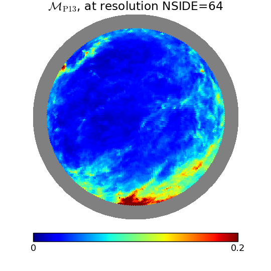
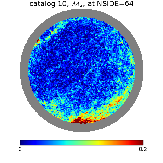
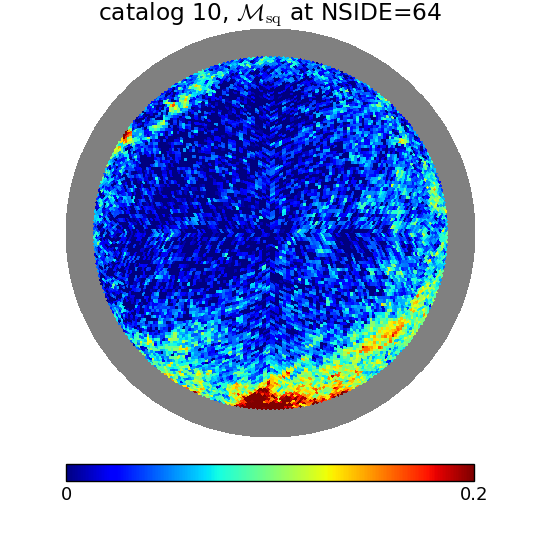
Figure 2 shows, for one mock catalog, orthogonal projections of maps of the true (P13) visibility mask and of the reconstructions ${\cal M}_{\rm av}$ and ${\cal M}_{\rm sq}$. The main large-scale features are neatly recovered, though noise is evident. A more quantitative analysis reveals that both reconstructions give a nearly unbiased estimate of the true mask for ${\cal M}\leq 0.1$, with a scatter that at this resolution amounts to $\sim$0.03 mag.

It is worth stressing that this level of agreement is obtained thanks to the second-order expansion of the integral in equation 2.12, the first-order expansion gives a much more biased estimate of the mask. A third-order expansion would likely improve the results at ${\cal M}>0.1$, but real large-scale surveys tend to avoid such relatively high extinction regions.

4.2 Combining ${\cal M}_{\rm av}$ and ${\cal M}_{\rm sq}$ into a best reconstruction of the mask

When applied to the density field computed on the native NSIDE=512 healpix grid, the two reconstructions show a much higher level of scatter at the pixel-by-pixel level. It is very instructive to analyse their angular power spectra. To this aim, we used the 20 mock light cones constructed with the procedure described in Section 3. Using the procedure described above in Section 3, we computed the angular density maps in redshift bins of width $\Delta z=0.1$ on a healpix grid of NSIDE=512, computed from these the $E_{\rm av}$ and $E_{\rm sq}$ estimators and used them to obtain ${\cal M}_{\rm av}$ and ${\cal M}_{\rm sq}$ by inverting equations 4.4 and 4.5. We used the implementation of the ANAFAST code provided by the Healpy package to compute the $C_{\ell}$ angular power spectra of the three reddening mask presented above and, for each mock, of the two reconstructed masks ${\cal M}_{\rm av}$ and ${\cal M}_{\rm sq}$. To account for the simple survey geometry, that encompasses $1/4$th of the sky, we multiplied all results by a factor of $4$. Figure 3 shows the results in terms of $\ell(\ell+1)C_{\ell}$. The green, blue and red lines give respectively the angular power spectra of the P13 “true” mask ${\cal M}_{\rm true}=E(B-V)_{\rm P13}$ and its two ${\cal M}_{\rm av}$ and ${\cal M}_{\rm sq}$ reconstructions; these are denoted by a band as thick as the standard deviation of measurements over the 20 realizations. The bands with lighter colors give the power spectra of reconstruction residuals, ${\cal M}_{\rm av}-{\cal M}_{\rm true}$ and ${\cal M}_{\rm sq}-{\cal M}_{\rm true}$. As a reference, we report in this plot (as a black continuous line) the measurement of angular clustering, averaged over our 20 light cones, of galaxies in the cosmological, unmasked samples at a fiducial redshift of $z=1.5$ (this signal includes shot noise). Because of a fortunate combination of matter clustering and halo bias, the level of this signal is pretty stable with redshift, so this line is representative of the expected level of clustering in the whole redshift range considered. The black dashed line gives for reference $1/100$th of the cosmological signal.

Figure 3: Angular power spectra of the true mask ${\cal M}_{\rm true}$ (green curve) and its reconstructions ${\cal M}_{\rm av}$ and ${\cal M}_{\rm sq}$ (blue and red curves). Reconstructions are averaged over the 20 light cones, the line width marks the standard deviation of the obtained clustering measurements. The cyan and pink lines give the power spectrum of the reconstruction residuals ${\cal M}_{\rm av}-{\cal M}_{\rm true}$ and ${\cal M}_{\rm sq}-{\cal M}_{\rm true}$. The black continuous line gives, as a reference, the measured clustering signal of galaxies at $z=1.5$, averaged over the 20 cosmological, unmasked mocks, and including shot noise. The dashed black line is $1/100$th of the previous curve. The lower panel gives the ratio between the two reconstructions and the true mask, and between the P15 and SFD masks and the true (P13) mask.

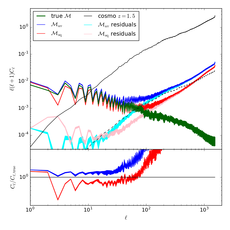
Both reconstructions reproduce the power spectrum of the mask at $\ell\,\hbox to0.0pt{\raise 2.15277pt\hbox{$<$}\hss}{\lower 4.30554pt\hbox{$\sim$}}\,30$, with a constant bias on large scales that amounts to $\sim 15$% for ${\cal M}_{\rm av}$ and $\sim 25$% for ${\cal M}_{\rm sq}$. At higher $\ell$’s the power spectra of reconstructions nose up to roughly follow the shape of the cosmological signal. The power spectra of reconstruction residuals are very informative to analyse. On very large scales they run parallel to the mask spectrum, while their raise at higher $\ell$-values is broadly parallel to the cosmological signal. This can easily be interpreted as the effect of incomplete averaging out of the cosmological signal. The $E_{\rm sq}$-based reconstruction gives lower residuals because the averaging is performed not over all redshift bins ($N_{z}=17$) but over all bin pairs ($N_{p}=136$) thus reducing the residual cosmological signal by a factor of 3, to a level that is more than a factor of $100$ below the cosmological signal. The $E_{\rm av}$-based reconstruction gives percent-level residuals for $\ell<100$.

Figure 4: Pixel-by-pixel scatterplots of reconstructed and true masks. In all panels grey dots denote pixel values, lines the average in bins of the quantity on the x-axis, the lighter-colored area the sample variance on the mean, errorbars the 16th and 84th percentiles in the same bins, averaged over the 20 mocks. The lower sub-panels give the residuals over the bisector line, denoted as a black line; here points are not reported. Upper panels: correlation of smoothed ${\cal M}_{\rm av}$ and ${\cal M}_{\rm sq}$ versus the true mask. Lower panels: correlation of the two smoothed reconstructions (left) and correlation of the best reconstruction with the true mask (right).

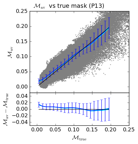
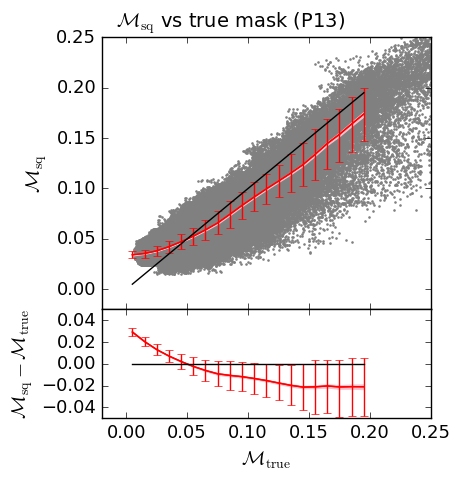
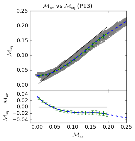
This result allows us to quantify the angular scales beyond which the reconstruction power spectra are dominated by the cosmological signal contamination. Notably, these scales will be valid as long as the foreground that contaminates a given survey has a power spectrum similar to the one used to create the mocks, that is biased toward larger scales. Because this excess small-scale power is correlated with the cosmological signal, it is important to filter it out. We do this by multiplying the $a_{\ell}^{m}$ coefficients of the spherical harmonics expansion of the reconstructed mask by a Gaussian smoothing function of $\ell$:

$$(a_{\ell}^{m})_{\rm smoothed,i}=(a_{\ell}^{m})_{i}\exp\left(-\left(\frac{\ell}{\ell_{i}}\right)^{2}\right)\,.$$ (4.6)

where $i={\rm av}$ or sq. Here the smoothing angular scales for the ${\cal M}_{\rm av}$ and ${\cal M}_{\rm sq}$ reconstructions, $\ell_{\rm av}$ and $\ell_{\rm sq}$, are kept separated to allow for a stronger filtering of the ${\cal M}_{\rm av}$ reconstruction, that is more contaminated by the cosmological residual. Good values for these smoothing scales are found to be $\ell_{\rm av}=90$ and $\ell_{\rm sq}=120$. In the following, we will only use the smoothed versions of the $E_{\rm av}$- and $E_{\rm sq}$-based reconstructions.

Figure 5: Orthogonal projections of the best reconstruction ${\cal M}_{\rm best}$ for the reconstructed mask (left panel), obtained with one of the mock catalogs, and of the true P13 reddening map used to mask the mock galaxy catalogs (right panel).

Figure 6: Angular power spectra of the true mask ${\cal M}_{\rm true}$ (green curve) and of the best reconstruction ${\cal M}_{\rm best}$ (orange curve). Reconstructions are averaged over the 20 light cones, the line width marks the standard deviation of the obtained clustering measurements. The light orange line gives the power spectrum of the reconstruction residuals ${\cal M}_{\rm best}-{\cal M}_{\rm true}$. The black continuous line gives, as a reference, the measured clustering signal of galaxies at $z=1.5$, averaged over the 20 cosmological, unmasked mocks. The dashed black line is $1/100$th of the previous curve. The lower panel gives the ratio between the reconstructions and the true mask.

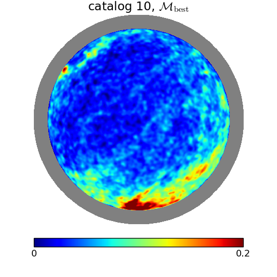
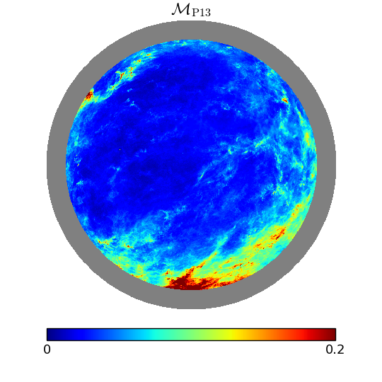
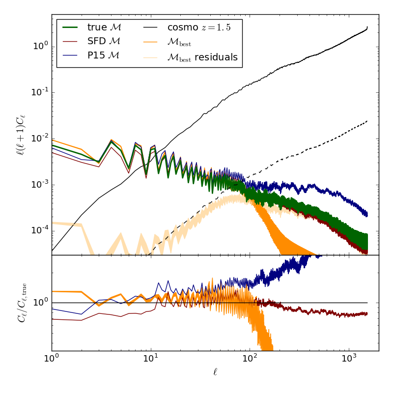
Figure 4 shows, in the two upper panels, the correlation between the two smoothed versions of the reconstructions with the true visibility mask ${\cal M}_{\rm true}$. Here the grey points represent the values obtained in all pixels in the survey for one single mock catalog; the lines give the mean of the reconstructed mask in bins of ${\cal M}_{\rm true}$, averaged over the 20 mocks, while the bands with lighter color around the mean give the sample variance (standard deviation) of the mean. Errorbars give the scatter of pixels in the same bins (quantified by the 16th and 84th percentiles), averaged over the 20 mocks. Residuals over the bisector line (denoted by a black line) are reported in the lower sub-panels. ${\cal M}_{\rm av}$ gives a remarkably unbiased reconstruction of the mask, with a bias below 0.01 mag with the exception of the very first point, and a scatter raising from 0.01 mag at low extinctions to 0.03 mag at ${\cal M}_{\rm true}=0.15$. ${\cal M}_{\rm sq}$ gives a more biased reconstruction, with an overestimate of 0.03 mag at the lowest reddening, turning negative beyond ${\cal M}_{\rm true}>0.05$; the scatter is lower than the ${\cal M}_{\rm av}$ case. The flattening of ${\cal M}_{\rm sq}$ at low extinctions is mostly due to the quadratic nature of the relation between the estimator $E_{\rm sq}$ and ${\cal M}_{\rm sq}$, that forces mask values to be positive.

It is convenient to combine the two reconstructions to obtain a nearly unbiased estimate of the mask with low residuals. One way could be to fix the bias of ${\cal M}_{\rm sq}$ by using the relation found with mocks; the accuracy of this reconstruction would depend much on how mocks have been constructed. A more conservative procedure can be built on the basis that we can directly measure the relation between the two reconstructions, and that this has a low scatter. This relation is shown in the lower left panel of figure 4. Using this relation, one can force one reconstruction to have the same bias as the other one, and because ${\cal M}_{\rm av}$ is nearly unbiased, we use this relation to transform ${\cal M}_{\rm sq}$. We fit the relation ${\cal M}_{\rm sq}=f({\cal M}_{\rm av})$ with a polynomial (extrapolated as a linear relation for ${\cal M}>0.2$), reported on the figure as a dashed line. This fit is performed only once, we checked that $f({\cal M}_{\rm av})$ is the same for all cases considered in this paper. We then correct ${\cal M}_{\rm sq}$ to have the same bias as ${\cal M}_{\rm av}$, that is known to be very low, by constructing the following “best reconstruction”:

$${\cal M}_{\rm best}={\cal M}_{\rm sq}-[f({\cal M}_{\rm av})-{\cal M}_{\rm av}]$$ (4.7)

Figure 4 gives, in the lower right corner, the correlation of ${\cal M}_{\rm best}$ with the true mask. It shows how this best reconstruction is biased in the same way as $M_{\rm av}$, i.e. by less than 0.01 mag, with the only exception of the first bin. The quality of the reconstruction can be appreciated in Figure 5, that shows the best reconstructed reddening map obtained with one specific catalog beside the original P13 map at the NSIDE=512 resolution used to mask the catalogs.

Figure 6 shows the angular power spectrum of the best reconstruction and its residual (the orange and lighter colored bands), compared with that of the true mask (in green). We compare these also to the angular power spectra of P15 and SFD masks (in dark blue and maroon respectively), as the differences between the masks can be taken as an order-of-magnitude indication of its uncertainty. The angular clustering is recovered by the best model in an almost unbiased way for $\ell<50$, while some gradual loss of power is present up to $\ell\sim 100$, where the reconstruction drops. This loss is mostly due to the lower value of the $\ell_{\rm av}$ smoothing scale; however, due to the higher contamination of ${\cal M}_{\rm av}$, a less strong smoothing would increase both power and residuals. This choice keeps the power spectrum of residuals well below 1%, thus avoiding significant correlation of signal and noise. If a better match of the power spectrum is needed, it would be better to use these simulations to increase high-$\ell$ power, boosting both signal and contamination, than increase $\ell_{\rm av}$, that would boost only the contamination.

5 Angular power spectra and cross correlations of density fields

5.1 The contribution of lensing

Figure 7: Left panels: angular correlation of the galaxy density field in redshift bins centered at $z=1$, $1.5$ and $2$, of width $\Delta z=0.1$. The green lines give the cosmological signal averaged over the 20 unmasked mock catalogs, the blue lines give the same measurement for catalogs masked with the P13 reddening map. Lighter-colored areas denote sample variance. The magenta dashed lines give the theoretical expectation including clustering, redshift-space distortions and lensing. Right panels: cross correlation of density fields at the same redshifts as above, with the same color coding.

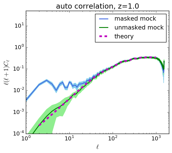
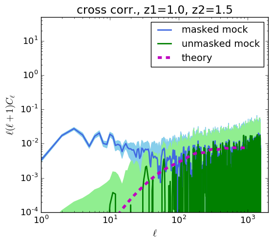
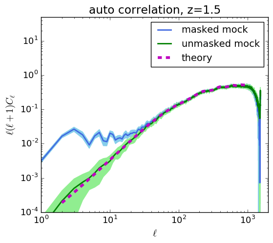
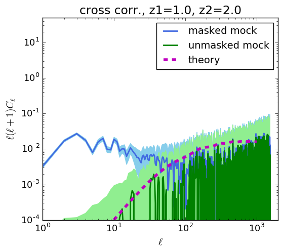
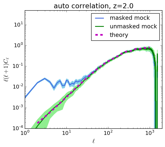
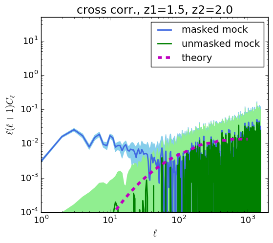
The reconstruction described in the previous sections relies on the assumption that the cross-correlation of cosmological signal in different redshift bins is vanishing. However, correlations in real data will be induced by gravitational lensing, mostly through magnification bias. This effect is not present in the mock catalogs that we are using for this analysis. To understand the expected influence of lensing, we show in figure 7 measured angular auto- (left panels) and cross- (right panels) correlation functions of galaxies at redshifts $z=1.0$, $1.5$ and $2.0$. In all panels the green and blue lines give the clustering of unmasked and masked catalogs, averaged over the 20 realizations, while the areas in lighter colors give the corresponding sample variance (quantified by the standard deviation over the 20 mocks). In the left panels the contribution of a Poissonian shot noise is subtracted from the signal, estimated as $4\pi f_{\rm sky}/N$, where $f_{\rm sky}=0.25$ is the fraction of the sky covered by the survey and $N$ is the number of galaxies in the redshift bin. The left-side column shows that the auto correlations of unmasked catalogs agree very well, as expected, with linear theory predictions, while masked catalogs show excess power at the same scale where the mask correlation is significant. On the right-side colum, the unmasked catalogs show cross-correlations consistent with noise around a vanishing value, while cross-correlations remain significant at $\ell<100$.

These measurements are compared with linear theory predictions, reported in the plots as magenta dashed lines. Linear theory predictions have been computed with classgal [43, 44, 45]. The redshift-dependent angular power spectra between $i$-th and $j$-th redshift bins are obtained as

$$c_{\ell}^{(ij)}=4\pi\int\frac{dk}{k}\Delta^{(i)}_{\ell}\left(k\right)\Delta^{(j)}_{\ell}\left(k\right)\mathscr{P}_{R}\left(k\right)$$ (5.1)

where $\mathscr{P}_{R}$ is the dimensionless primordial curvature power spectrum and $\Delta_{\ell}^{(i)}\left(k\right)$ is the full angular transfer function in the $i$-th redshift bin. In this work we consider the main contributions, namely density, redshift space distortion (RSD) and lensing convergence defined as follows:

$$\Delta_{\ell}^{\delta(i)}\left(k\right) = \int dr\ W_{i}\left(r\right)b_{1}T_{\delta}\left(k,r\right)j_{\ell}\left(kr\right)\,,$$ (5.2)

$$\Delta_{\ell}^{{\rm rsd}(i)}\left(k\right) = \int dr\ W_{i}\left(r\right)\frac{k}{aH}T_{v}\left(k,r\right)j^{\prime\prime}_{\ell}\left(kr\right)\,,$$ (5.3)

$$\Delta_{\ell}^{\kappa(i)}\left(k\right) = \ell\left(\ell+1\right)\int dr\ W_{i}\left(r\right)\int_{0}^{r}dr^{\prime}\frac{2-5s}{2}T_{\Phi+\Psi}\left(k,r^{\prime}\right)j_{\ell}\left(kr^{\prime}\right)\,,$$ (5.4)

where the Fourier transfer functions $T\left(k,r\right)$ are normalized to the primordial curvature perturbation and they refer, respectively, to density, velocity and Bardeen potentials, $j_{\ell}$ are the spherical Bessel functions and $j^{\prime\prime}_{\ell}$ their second derivative with respect to the argument. The redshift binning is denoted by the function $W_{i}$, normalized to unity. The shape of $W_{i}$ is assumed to take into account redshift errors; here we are assuming no error on spectroscopic redshift, so we used a shape very near to a square window function, checking that results are insensitive to further sharpening.

Linear predictions depend on the galaxy bias $b_{1}(z)$ and the magnification bias $s(z)$. Here the bias is assumed to be independent of luminosity, so these predictions are comparable with our mocks where the luminosity dependence of bias has been removed by shuffling halo masses (see Section 3). Linear bias $b_{1}$ was obtained as explained in Section 3 and is reported in figure 1, magnification bias $s(z)$ is defined as the logarithmic slope of the luminosity function at the threshold luminosity, so $s(z)=2S_{B}(z)-1$.

The upper panels show that the clustering of cosmological unmasked catalogs follows very closely linear theory, despite missing the lensing term. This is no surprise, because the contribution of lensing (whose level is appreciable in the right panels) is negligible for auto correlations with respect to clustering and RSD for redshift bins of the width $\Delta z=0.1$ (see e.g. [46]). This is not the case for cross correlations, where the expectation for clustering and RSD is very low, and the signal is dominated by lensing, that is missing in the mock catalogs. For the masked mocks, expected lensing and measured cross correlation cross at $\ell\sim 50-100$, after which lensing follows the envelope of the wide fluctuations. This illustrates once again that the importance of a foreground like Milky Way extinction is limited to the largest angular scales.

5.2 Reconstructing the true angular clustering

The customary way to correct for a given foreground is to create a random catalog that is subject to the same selection bias as the measured one. This would be straigthforward to implement, and would make it possible to measure clustering in redshift space and assess how well the cosmological clustering signal is recovered. We leave this project to future work, and test here only the recovery of angular clustering. Equation 2.20, that relates the observed density contrast with the matter one, can be inverted if the mask ${\cal M}$ is known or a reconstruction for it is available. The process is more complicated for the general case of luminosity-dependent bias, but if luminosity dependence is absent, as in our mock catalogs based on shuffled halo masses, then $b_{1}=\beta_{1}$ and $\beta_{1}^{\prime}=0$, so the inversion is easily performed:

$$1+\delta_{\rm g}=\left[1+\frac{S_{C}}{S_{A}}\left(1+\frac{S_{C}}{S_{A}}{\cal M}\right)({\cal M}-\langle{\cal M}\rangle)+\frac{S_{B}S_{C}^{2}}{S_{A}}({\cal M}^{2}-\langle{\cal M}^{2}\rangle)+O({\cal M}^{3})\right](1+\delta_{\rm o})$$ (5.5)

Figure 8: Reconstructed angular correlation of masked catalogs at redshifts $z=1.0$ (upper left), $1.5$ (upper right), $2.0$ (lower left) and $2.4$ (lower right). In the main panels the green and blue lines give the angular clustering of unmasked and masked catalogs, ligher colored areas giving the sample variance. Orange, black, dark blue and maroon lines give the average of the reconstructed angular correlation using respectively the best reconstruction, the true P13 mask, the P15 and SFD masks. The lower panels give the residual with respect to the average true correlation of the unmasked mocks, the lighter coloured areas give the sample variance of the ratio of reconstructed and true clustering using the true mask (gray) and the best reconstruction (orange).

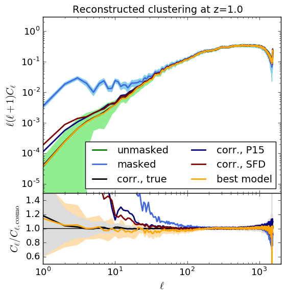
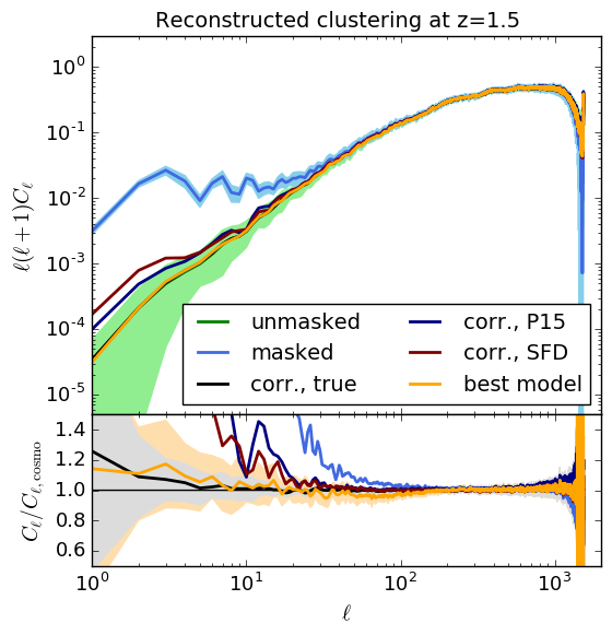
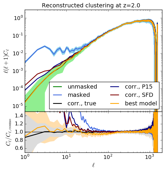
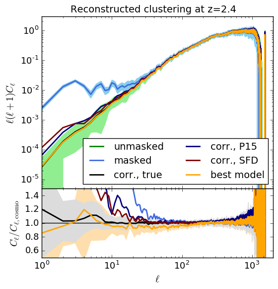
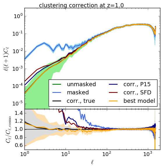
Figure 8 shows the angular power spectra of galaxy density contrasts computed using equation 5.5, at redshifts $z=1.0$, $1.5$, $2.0$ and $2.4$. The bright blue and green lines show respectively the angular power spectrum of the (masked) observed density contrast $\delta_{\rm o}$ and of the true galaxy density contrast $\delta_{\rm g}$, the lighter-colored areas around them give their sample variance (as in figure 7). The recovery of the true galaxy power spectrum is performed using the true P13 mask (black lines), the P15 (dark blue lines) and SFD (maroon lines) masks, and the best reconstruction (orange lines). For each panel, the lower sub-panel shows the ratio of the reconstructed power spectrum over the one of the unmasked catalog, i.e. the quantity to recover. Lighter-colored gray and orange areas give the sample variances of the ratios obtained with the true mask and with the best reconstruction.

Figure 9: Ratio of sample variance over signal for the true angular power spectrum of galaxies (green line), for the ratio between reconstructed and true power spectrum using the true mask (gray line) and the best reconstruction (orange line).

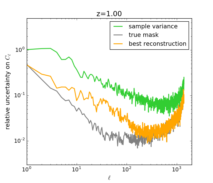
An important thing to notice is that the recovery of the true galaxy density field is affected by some uncertainty even when the true mask is used; this is due to the statistical nature of the correction applied to the observed density contrast. To have a better quantification of this, figure 9 reports, for the first redshift $z=1.0$ (other redshifts give very similar results), the ratio of variance over signal for the cosmological angular power spectrum and for the ratios of the two reconstructions (with the true mask and with the best reconstruction). The uncertainty in the reconstruction obtained with the true mask is always nearly a factor of ten below sample variance, raising to higher values only at high $\ell$’s, when the shot-noise-subtracted signal drops. The best reconstruction carries a higher uncertainty by a factor of 3, that is anyway lower by another factor of 3 than the sample variance; however, it must be kept in mind that this bias is systematic, and cannot be decreased by averaging over several $\ell$’s.

As for averages, correcting with the true mask always gives an unbiased reconstruction of the power spectrum, while correcting with other masks gives results that significantly deviate from the true clustering at low $\ell$’s; compared with the clustering of the masked catalogs, correcting densities with the “wrong” mask gives an improvement of only a factor of $\sim 3-4$ in terms of the $\ell$ at which clustering deviates significantly from the true solution. Clearly deviations from true clustering are much less dramatic than the option of not correcting at all, yet deviations at low $\ell$’s go beyond the sample variance of the measurement.

The best reconstruction gives on average a remarkably unbiased estimate down to very low $\ell$’s. Sample variance is important at the largest angular scales, but always at the level of $\sim 20$ % and below sample variance by a factor of 3. At $\ell=30-50$ we find a systematic underestimation of $\sim 5$ %; it is plausible that this bias could be removed by working on the combination of $E_{\rm av}$ and $E_{\rm sq}$ estimators, we leave this refinement to future work.

5.3 Cross correlations as a blind test for the mask

Figure 10: Angular cross-correlation of masked catalog for $z_{1}=1.0$ and $z_{2}=2.0$. The green and blue line gives the average measurement of the masked catalog, lighter blue areas gives its sample variance (16th and 84th percentiles). Orange, black, dark blue and maroon lines give the average of the predicted cross-correlation using respectively the best reconstruction, the true P13 mask, the P15 and SFD masks. The lower panels give the residual with respect to the average true cross correlation.

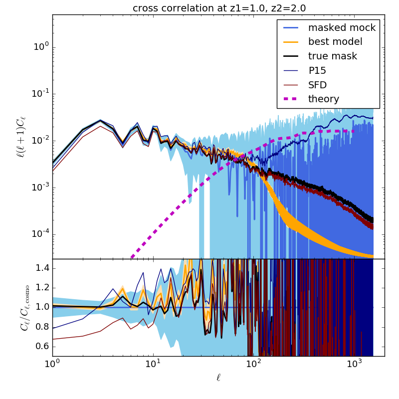
The cross-correlations of $\delta_{{\rm o}1}\equiv\delta_{\rm o}(\bm{\theta}_{1},z_{1})$ and $\delta_{{\rm o}2}\equiv\delta_{\rm o}(\bm{\theta}_{2},z_{2})$ for $z_{1}\neq z_{2}$ will depend only on the mask term, so it is possible to predict them, given the mask reconstruction. Calling ${\cal M}_{1}={\cal M}(\bm{\theta}_{1})$ and ${\cal M}_{2}={\cal M}(\bm{\theta}_{2})$:

$$\langle\delta_{o1}\delta_{o2}\rangle = F_{1}F_{2}\,\langle({\cal M}_{1}-\langle{\cal M}\rangle)({\cal M}_{2}-\langle{\cal M}\rangle)\rangle+(F_{1}G_{2}+F_{2}G_{1})\langle({\cal M}_{1}-\langle{\cal M}\rangle)({\cal M}^{2}_{2}-\langle{\cal M}^{2}\rangle)\rangle$$ (5.6)

$$+G_{1}G_{2}\,\langle({\cal M}_{1}^{2}-\langle{\cal M}^{2}\rangle)({\cal M}^{2}_{2}-\langle{\cal M}^{2}\rangle)\rangle$$

$$F_{i} = \frac{S_{Ci}}{S_{Ai}}\left(1+\frac{S_{Ci}}{S_{Ai}}\langle{\cal M}\rangle\right)\,,\ \ \ \ \ \ \ \ \ \ \ G_{i}=\frac{S_{Bi}S_{Ci}^{2}}{S_{Ai}}$$

Figure 10 shows, as an example, the cross correlation of observed density at redshifts $z_{1}=1.0$ and $z_{2}=2.0$. The blue line gives the average measurement, the lighter blue area its sample variance. Black, dark blue, maroon and orange lines give the predicted cross correlation based respectively on the true mask, P15, SFD and the best reconstruction, the last with its sample variance. While the black line unsurprisingly gives the right level of correlation, the best reconstruction (orange line) gives again a remarkably unbiased prediction of this correlation, while the same is not true for P15 and SFD masks, that show sizeable discrepancies in various $\ell$ ranges.

At the largest scales, while auto-correlations are dominated by the foreground, for cross correlations this is the only contributing term. In this paper we have constructed estimators of the non cosmological term of observed density contrast, used them to reconstruct the mask, and used the reconstructed mask to check that observed cross correlations are correctly predicted. This logical progression could have been reversed: we could have started from the measured cross correlations of observed density contrast and use it to infer the angular power spectrum of the mask. These two quantities are related to the mask through equation 5.6, that however includes correlations of the terms ${\cal M}-\langle{\cal M}\rangle$ and ${\cal M}^{2}-\langle{\cal M}^{2}\rangle$. Even assuming knowledge of the first two moments of the mask, it is not straightforward to invert this relation to obtain $\langle{\cal M}_{1}{\cal M}_{2}\rangle$. The presence of square terms of the mask in that equation is due to the second-order expansion of the integral in equation 2.12, and we know that a first-order expansion, that would make the direct measurement of the angular power spectrum of the mask possible, is not sufficiently accurate.

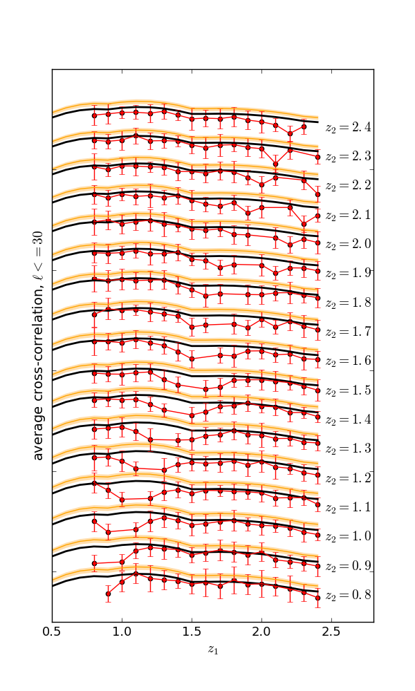
To better quantify the level of agreement with which cross correlations are recovered, we measure the average of $\ell(\ell+1)C_{\ell}$ in the multipole range $\ell\leq 30$, where the signal is strongest and sample variance is still limited (figure 10). Figure 11 shows such average cross correlation for all redshift pairs $z_{1}$ and $z_{2}$. Here the dots show the average over 20 mocks and the errorbars give their sample variance. Measurements are shown as a function of $z_{1}$, points at fixed $z_{2}$ are displaced vertically to ease the comparison, so vertical values are arbitrary. Points corresponding to auto-correlations, with $z_{1}=z_{2}$, are not shown because they are obviously affected by the cosmological signal. The black and orange lines give the predictions obtained with the true mask and the best reconstruction, for the latter we report its sample variance as a lighter colored area. The prediction based on the true mask (black line) follows well the data points; we computed a reduced $\chi^{2}$ to test if the differences are significant, and found some systematics due to nearby redshift bins, that show some degree of anti-correlation of putative cosmological origin, and to the last bin, hinting to some possible weakness in the mock construction near the edge of the light cone. Excluding these bins (so limiting then the analysis to 91 bin pairs), we found acceptable values of the reduced $\chi^{2}$, though the prediction is biased high on average by 3%.

Being the cosmic correlation not exactly vanishing for nearby redshift bins, these could be removed from the estimate of $E_{\rm sq}$ to achieve a cleaner reconstruction; however, this advantadge would be counterbalanced by an increase of the residuals due to imperfect averaging out; given that cosmic correlation has in figure 11 just an effect at the $2\sigma$ level, compared to sample variance, we prefer here to keep a larger number of bin pairs. We plan to deepen the effect of these correlations in future work.

Predictions of cross correlations based on the best reconstruction show some mild discrepancy, that is quantified as a reduced $\chi^{2}$ of $\sim 2$ for 91 measurements defined above. Predictions are biased high by 10%, that is at the level of $1\sigma$ but is systematic on all measurements. As shown in the previous sections, the practical effect of this bias is very small, but because cross correlations can be measured, this bias can in principle be removed by further calibrating the reconstruction scheme to best reproduce the average cross correlations. One possibility could be to use this constrain to measure at least one of the two moments of the mask; however the mask enters equation 5.6 through ${\cal M}-\langle{\cal M}\rangle$ and ${\cal M}^{2}-\langle{\cal M}^{2}\rangle$, so cross correlations are insensitive to the values of $\langle{\cal M}\rangle$ and $\langle{\cal M}^{2}\rangle$. We checked that it is possible to obtain unbiased cross correlations by increasing $\langle{\cal M}\rangle$ by 0.04, leading to an almost doubled, unacceptable value. Conversely, a multiplicative fudge factor applied to the reconstructed mask of $0.97$ can make the predictions of the cross correlations as (nearly) unbiased as those produced with the true mask, with negligible impact on the pixel-by-pixel correlation of figure 4.

We conclude this section stressing that, whatever the mask model or reconstruction scheme is, cross correlations provide a blind test for foreground removal. Suppose all known foreground corrections have been applied to a deep galaxy sample, then one would expect cross correlations to be consistent with a vanishing signal (quantified through mocks), so a significantly non-vanishing value would show that foreground removal is not complete. The angular power spectrum of the cross correlations would immediately give clues on the nature of this foreground, one could then calibrate the weights of the various components to minimise the residual cross correlations, then apply the reconstruction scheme presented here to model the missing residual, and quantify its uncertainty using mock catalogs.

Figure 11: Average value of the cross correlation power spectrum $C_{\ell}$, for $\ell\leq 30$, of pairs of masked density fields at redshifts $z_{1}$ and $z_{2}$, as a function of $z_{1}$ and for all $z_{2}$. Points and curves are displaced vertically to distinguish the curves. Red points and errorbars give its average measurement (over the 20 mock catalogs) and sample variance (standard deviation). Black and orange lines give the predicted value using the true P13 mask and the best reconstruction, results obtained with the “wrong” P15 and SFD masks are not shown for sake of clarity, but deviate significantly from the measurements.

6 Estimating $\langle{\cal M}\rangle$ and $\langle{\cal M}^{2}\rangle$

Figure 12: Angular clustering of best reconstruction for the mask (left panels) and reconstructed angular clustering of galaxies (right panels) for reconstructions that use $\langle{\cal M}\rangle$ and $\langle{\cal M}^{2}\rangle$ from P15 (upper panels) and SFD (lower panels). Symbols and colors are as in figures 6 and 8.

The results presented up to now rely on prior knowledge of the first two moments of the mask, $\langle{\cal M}\rangle$ and $\langle{\cal M}^{2}\rangle$. We demonstrate in this section that it is possible to recover this information either from external sources or internally, without compromising the effectiveness of the method.

Map	true	estimated	diff.	true	estimated	diff.
	$\langle{\cal M}\rangle$	$\langle{\cal M}\rangle$		$\langle{\cal M}^{2}\rangle$	$\langle{\cal M}^{2}\rangle$
P13	0.0474	0.0453	4.5%	0.00356	0.00350	1.7%
P15	0.0451	0.0457	1.1%	0.00382	0.00370	3.1%
SFD	0.0396	0.0417	5.5%	0.00277	0.00289	4.2%

Table 1: Values of the first two moments of the masks, and estimated values using the procedure described in this section.

As a first step, we test the degradation of the results obtained using the first two moments computed from a different reddening map, P15 or SFD. When computed on the same sky area, the three maps give values of $\langle{\cal M}\rangle$ that differ at most by 20%, and values of $\langle{\cal M}^{2}\rangle$ that differ at most by 38%. These figures are reported in table 1; we can take their difference as an order-of-magnitude indication of their measurement error. Figure 12 shows the angular power spectrum of the reconstructed mask (left figures, similar to figure 6) and the reconstructed galaxy angular clustering (right figures, similar to figure 8) at $z=1$, obtained using the values of the two moments from P15 or SFD, in place of the true ones. Results show clearly that using the “wrong” values of the first two moments leads to nearly indistinguishable results; the most remarkable difference is seen at the largest scales, where the lower power of the SFD mask happens to compensate the slight overestimate of the mask power spectrum noticeable in figure 11, thus beating down the residuals.

As mentioned above, the reason why results are insensitive to exact values of the moments is visible in equation 5.6: the mask enters this equation for the cross correlation through ${\cal M}-\langle{\cal M}\rangle$ and ${\cal M}^{2}-\langle{\cal M}^{2}\rangle$, plus a $\langle{\cal M}\rangle$ term in the $F_{i}$ coefficients, so a constant bias in the 1st moment of the mask has only 2nd-order effects on the cross correlation, and consequently in the ability to subtract the contamination from the cosmological signal, while a bias in the 2nd order moment will have 3rd-order effects that are neglected here.

Figure 13: Left panel: average residuals of the ${\cal M}_{\rm av}$ reconstruction (as the lower sub-panels of figure 4 for mocks masked with the three reddening maps (P13, dark blue; P15, green; SFD, maroon), as a function of the true mask ${\cal M}_{\rm true}$ (different for the three cases). Continuous lines: $\langle{\cal M}\rangle$ and $\langle{\cal M}^{2}\rangle$ are computed from the true mask; the lighter-colored areas give the sample variance of the mean. Dotted lines: the same as the continuous line, shifted down by the corresponding value of $\langle{\cal M}\rangle$. Dashed lines: reconstruction computed with $\langle{\cal M}\rangle=0$ and $\langle{\cal M}^{2}\rangle=0$. Right panel: cumulative fraction of pixels as a function of reddening. Colors are as for the left panel, continuous lines give the true masks, dashed lines give results for ${\cal M}_{\rm av}$ reconstructions with $\langle{\cal M}\rangle=0$ and $\langle{\cal M}^{2}\rangle=0$. The black horizontal line marks the fiducial $10^{-2}$ level chosen in the text, the vertical line gives the $0.008$ value of ${\cal M}_{1\%}$ (below which we have 1% of sky pixels), the other segments mark the expected position of ${\cal M}_{1\%}$ for the $E_{\rm av}$-based reconstructions.

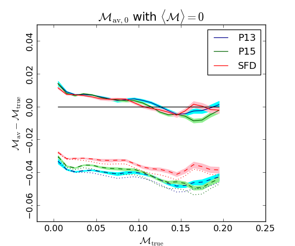
We further show that it is possible to recover $\langle{\cal M}\rangle$ and $\langle{\cal M}^{2}\rangle$, to sufficient accuracy, from an internal analysis of the survey data and some calibration on the mock catalogs. To this aim we consider the $E_{\rm av}$-based ${\cal M}_{\rm av,0}$ reconstruction, applied to the survey assuming zero values for the two moments. This is equivalent to applying the $E_{\rm av}$ estimator, equation 4.4, directly to the observed density $\delta_{\rm o}$ (equation 2.20) in place of the rescaled $\delta_{\rm r}$ (equation 4.2). At leading order in ${\cal M}$, adequate for the least reddened sky pixels, it is easy to demonstrate that $M_{\rm av,0}={\cal M}-\langle{\cal M}\rangle$, so a mask reconstruction obtained assuming $\langle{\cal M}\rangle=0$ is shifted, with respect to the true mask, exactly by $\langle{\cal M}\rangle$. This is shown on the left panel of figure 13, where we report the average (and sample variance) of ${\cal M}_{\rm av}-{\cal M}_{\rm true}$ obtained using the mocks masked with the three P13, P15 and SFD masks, assuming exact knowledge of the moments (the continous lines surrounded by lighter colored areas) and zero moments (the dashed lines surrounded by lighter colored areas). The quantities reported in this figure are analogous to the residuals of ${\cal M}_{\rm av}$ shown in the upper left panel of figure 4 (without the errorbars used to denote the scatter). It is worth highlighting that to produce this figure we used mock catalogs masked with the three reddening maps, and for each set of mocks we compare results with the corresponding true map. The dotted lines here are the continuous lines shifted by the corresponding value of $\langle{\cal M}\rangle$; they are shown to demonstrate that the shift is very similar to the first moment of the mask.

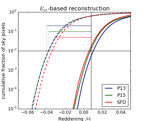
Unfortunately, the quantity reported in figure 13 is not observable. We therefore identify a procedure to get a good estimate of $\langle{\cal M}\rangle$. In the right panel of figure 13 we report the cumulative distribution of reddening values obtained with ${\cal M}_{\rm av}$ applied to mocks masked with the three reddening maps, both using the true $\langle{\cal M}\rangle$ (continuous lines) and using $\langle{\cal M}\rangle=0$ (dashed lines). These cumulative distributions are very robust to sample variance, so we just show the average curve. To quantify the shift we choose a bona fide fraction of $10^{-2}$, and quantify from mocks that this fraction is obtained at ${\cal M}\simeq 0.008$ for the three masks used. We define an estimate $\langle{\cal M}\rangle_{\rm est}$ of the first moment as the distance between 0.008 and the ${\cal M}_{1\%}$ value below which we find 1% of sky pixels:

$$\langle{\cal M}\rangle_{\rm est}=-{\cal M}_{1\%}+0.008\,.$$ (6.1)

The obtained values are reported in table 1, and are accurate to within 5.5% at worst. This demonstrates that such an internal procedure, calibrated on mock catalogs, gives a potentially more accurate estimate than using an external model for the map.

The estimate of $\langle{\cal M}^{2}\rangle$ is even less problematic, because the reconstruction is not very sensitive to its exact value. Once $\langle{\cal M}\rangle$ has been fixed, a very good estimate is obtained by finding the best reconstruction ${\cal M}_{\rm best0}$ assuming a vanishing value of $\langle{\cal M}^{2}\rangle$, then using the value of $\langle{\cal M}_{\rm best0}^{2}\rangle$. We find such values to be biased high, for all three maps, by a constant $0.0007$, that is broadly consistent with the idea that the final square average is the sum of the true one and the squared scatter around the mean, quantified here as $\sqrt{0.0007}=0.026$ mag. Using this mock-calibrated fix, we obtain:

$$\langle{\cal M}^{2}\rangle_{\rm est}=\langle{\cal M}_{best0}^{2}\rangle-0.0007\,.$$ (6.2)

The average values of this estimate for the three maps are reported in the table; they are found to be within $\sim 4.2$% of the true value, a very adequate level of accuracy.

Figure 14: Performance of the best reconstruction obtained by estimating the first two moments of the mask from internal data. Upper left panel: angular power spectrum of the mask, as in figure 6. Upper right panel: pixel-by-pixel scatterplot of reconstructed and true masks, as in the lower right panel of figure 4. Lower left panel: reconstructed galaxy angular power spectrum at $z=1$, as in figure 8. Lower right panel: Angular cross correlation between $z=1$ and $z=2$, as in figure 10.

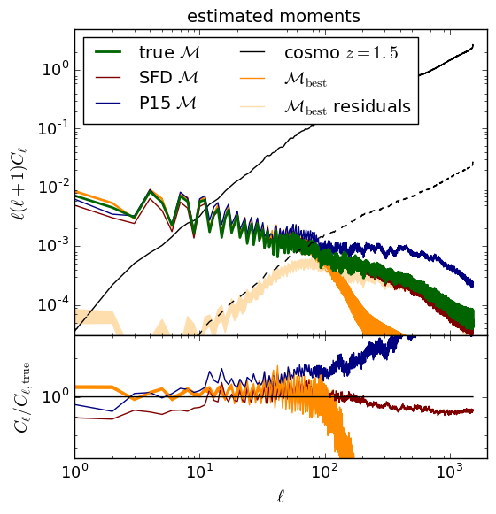
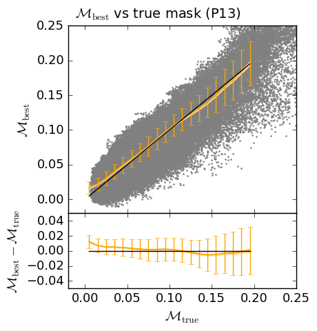
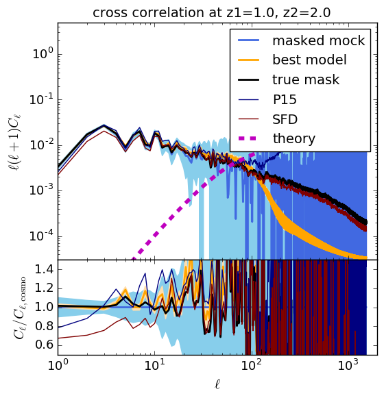
We are now in the position to present the best reconstruction of the mask assuming no prior knowledge of its moment. We implement this procedure: (i) the $E_{\rm av}$ estimator and ${\cal M}_{\rm av}$ are computed assuming $\langle{\cal M}\rangle=\langle{\cal M}^{2}\rangle=0$; (ii) equation 6.1 is used to obtain an estimate of $\langle{\cal M}\rangle$; (iii) the best reconstruction is constructed assuming $\langle{\cal M}^{2}\rangle=0$; (iv) equation 6.2 is used to obtain an estimate of $\langle{\cal M}^{2}\rangle$; (v) the best reconstruction is recomputed. One could further multiply the result by $0.97$ to optimize the reproduction of the observed cross correlations (Section 5.3). Figure 14 shows the main results of the reconstruction: angular power spectrum of the mask (as in figure 6), pixel-by-pixel scatterplot of reconstructed and true masks (as in figure 4), reconstructed correlation of the cosmic signal at $z=1$ (as in figure 8) and predicted cross correlation between $z=1$ and $z=2$ (as in figure 10). None of the results is found to suffer a degradation of accuracy.

7 Testing reddening maps

Figure 15: Upper panels: pixel-by-pixel scatterplots of the best reconstruction, obtained with mocks masked with the P13 reddening map, as a function of P15 or SFD reddening. Symbols and colors are as in figure 4. Lower panels: relation between P13, P15 and SFD maps; here averages are of course computed for a single realization, so no sample variance is reported.

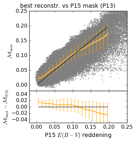
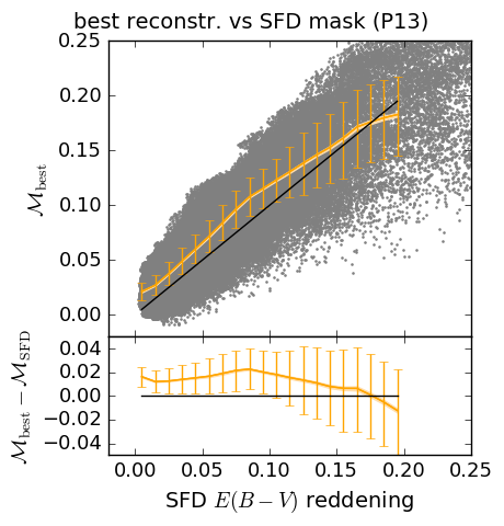
The results presented above demonstrate that the technique described in this paper can recover the reddening map with a precision that is comparable, and sometimes competitive, to the difference between available reddening maps. The argument in principle can be reversed: if extinction is the only foreground, reddening maps, obtained as reconstructed foreground masks from deep and wide galaxy surveys, can be used to constrain and test models for galaxy extinction, and thus help in shedding light on the complex physics of dust in the solar neighborhood. We have already shown evidence in this sense: figure 6 shows that the reconstructed power spectrum of the mask is more compatible with the P13 power spectrum than with the other two, P15 showing some power excess at $\ell\sim 100$ and SFD some lack of power at the largest angular scales. Figure 10 shows that cross correlations are predicted to better accuracy by the best reconstruction than by the P15 and SFD masks. If reported in figure 11, predictions of P15 and SFD systematically lie above (P15) and below (SFD) the measured values. It is important to stress that this cross correlation test alone, that is completely independent of the reconstruction procedure, would be enough to test reddening maps and assess the one that best fits the data.

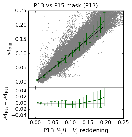
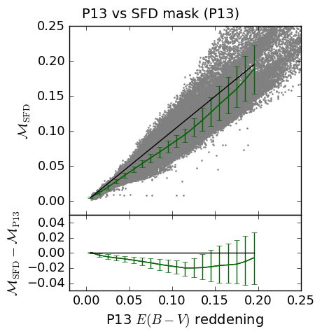
The same conclusion holds true at the pixel-by-pixel level. Figure 15 shows the scatterplots of the best reconstructions, as in figure 4, compared with the P15 and SFD masks. For reference, the lower panels show the scatterplot of P13 versus P15 and SFD. It is clear that, despite of the higher level of scatter, the agreement of the best reconstruction with the true P13 mask is better than the agreement with the other two masks. This evidence alone would be enough to disfavour SFD, while P13 and P15 are nearly unbiased due to the very similar calibration on quasars, and so are more difficult to distinguish with this test.

The weak point of this program is that it relies on the assumption, true for our mock catalogs, that galactic extinction is the only foreground that affects the survey. This will clearly not be the case in general, and other foregrounds, for example contamination from field stars, may be confused with extinction. However, different foregrounds may be characterised by different $S_{C}$ scaling functions, that quantify the redshift modulation of the impact of the foreground. Two foregrounds that have proportional $S_{C}$ functions, e.g. a redshift-independent constant, would not be separable; in the case of $H\alpha$ emitters considered here, the effect of galactic extinction is modulated in a peculiar way by the extinction curve $R(\lambda)$, so its separation from other components is possible.

Figure 16: Average value of the cross correlation power spectrum $C_{\ell}$, for $\ell\leq 30$, of pairs of masked density fields at redshifts $z_{1}$ and $z_{2}$, as a function of $z_{1}$ and for all $z_{2}$. Symbols are as in figure 11, but best reconstruction predictions (orange lines) have been produced here by assuming a flat $S_{C}(z)$ function.

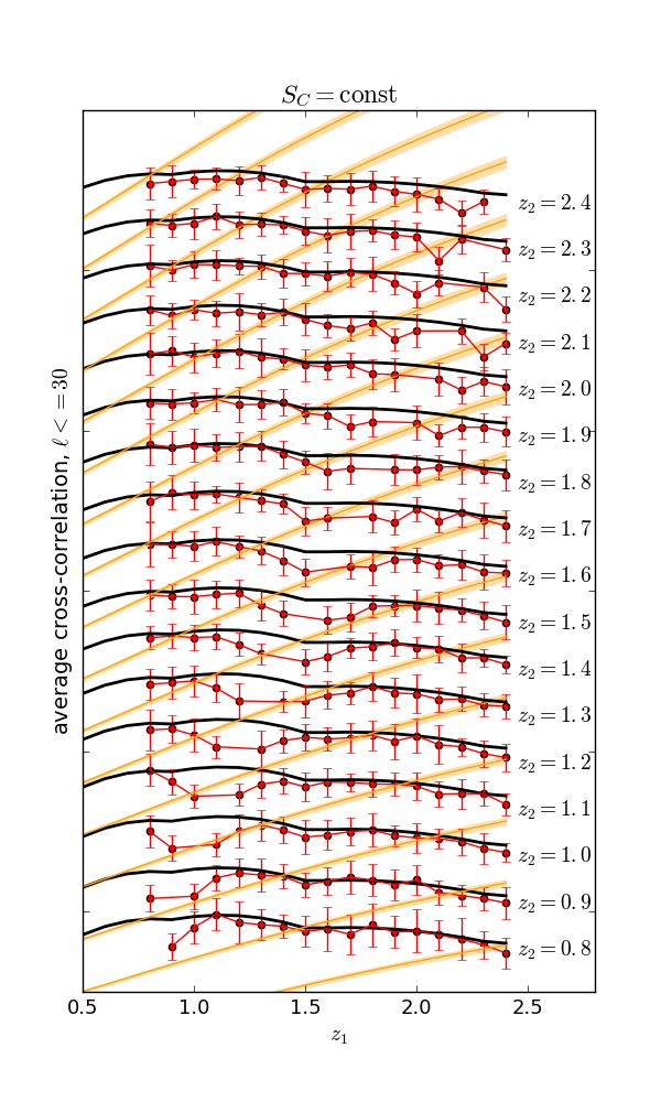
The way to break the degeneracy between different foregrounds is to fully exploit the ability to predict cross correlations at large scales, e.g. as quantified in figure 11. As an example, we show in figure 16 the prediction of cross correlations performed assuming a flat $S_{C}(z)$ function. While the angular maps result very similar, the predicted redshift dependence of cross correlations is in stark disagreement with observations. It would be easy to assume a functional form for $S_{C}(z)$ (e.g. a polynomial) and obtain the coefficients from fitting cross correlations; we plan to test this procedure in the future.

8 Conclusions

In this paper we have proposed a blind method to determine the properties of a foreground contamination that affects a deep galaxy survey. As a prototypical foreground, we have considered Milky Way extinction, and used three different extinction maps (Schlegel et al’s SFD and the two P13 and P15 Planck maps) available in the literature. We have developed the method and tested its validity using a set of 20 mock halo catalogs generated with the PINOCCHIO code. We have simulated an Euclid-like survey of $H\alpha$ emitters covering $1/4$th of the sky in the redshift range $0.75<z<2.45$, by abundance-matching the halo mass function with the luminosity function of model 1 of Pozzetti; this way the impact of the foreground is modulated in redshift by the extinction curve.

The method we propose is based on the fact that (i) foregrounds act in modulating the flux limit of the galaxy survey, (ii) cross correlations of galaxy density fields in different redshift bins have a small cosmological contribution, dominated by lensing at $\ell>100$ and vanishing at larger angular scales. By expanding to second order of flux modulation the observed number density of galaxies, we have shown that the measured signal of cross correlations can be associated to a foreground mask. We have identified two estimators, the average density contrast $E_{\rm av}$ of a sky pixel along the line of sight and the average $E_{\rm sq}$ of products of density contrasts at different redshift bins in the same sky pixel, that average out (in an ensemble-average sense) the cosmological signal, and single out a contribution that depends only on the foreground mask. Assuming that the first two moments of the foreground mask are known, it is possible to relate these estimators to polynomials of the mask, that can be easily inverted to reconstruct the visibility mask.

This reconstruction technique would be applied to a real survey as follows. (i) The luminosity function at the survey flux limit should be known with great detail from a deep field, so as to determine $S_{A}(z)$ and $S_{B}(z)$. (ii) Luminosity dependence of bias can be measured, up to a constant, by computing how the two-point correlation function (or power spectrum) changes when the sample is selected with an increasing flux limit. (iii) The $S_{C}(z)$ function must be first assumed, under some plausible hypothesis. (iv) The density contrast field is computed for each redshift bin. (v) The $E_{\rm av}$ and $E_{\rm sq}$ estimators are computed, the corresponding masks are obtained by inverting equations 4.4 and 4.5 and the best reconstruction ${\cal M}_{\rm best}$ is obtained through equation 4.7. (vi) The cross-correlation test is applied to the obtained mask to validate the assumed $S_{C}(z)$ function, if a good match is not found point (v) is iterated using some parameterization of this function, until a good fit of cross correlations is found. (vii) The mask thus obtained is used to produce a random catalog for clustering statistics. (viii) The mask can also be used to straightforwardly obtain the galaxy density contrast on the sky and the galaxy angular power spectrum using equation 5.5.

In the plausible case that different foregrounds, characterized by different $S_{C}(z)$ functions, are present at the same time, the method should be extended to take this higher complexity into account. Such extension is straightforward, and it would possibly benefit from the application of Bayesian inference methods based on forward modeling, as that proposed, e.g., by [20].

The reconstructed foreground mask reproduces very well, on relatively large angular scales ($\ell<100$), the properties of the reddening map used to mask the mock catalogs (P13), at a level that would make it possible to distinguish it form P15 or SFD: extinction is recovered at the pixel-by-pixel level with a bias that is below $0.01$ mag, and a scatter ranging from $0.01$ to $0.03$ mag, slightly growing with reddening. The reconstructed mask is smoothed in spherical harmonic space at $\ell\sim 100$, to remove the small-scale signal that is dominated by the imperfect averaging out of the cosmological signal, due both to the limited number of redshift bins and to the use of volume averages in place of ensemble averages. The so-obtained reconstruction of the mask can be used to remove the spurious power from the angular correlation function. We showed that this removal gives unbiased results up to $\ell$ of a few, where the cosmological signal is two orders of magnitude below the contamination, with a statistical uncertainty of $\sim 20\%$, a (systematic) factor of 3 below the sample variance of the observable. This technique can then have an impact on constraints on primordial non-gaussianities, whose measurement is limited by sample variance, thoug constraints can be improved by adopting multi-tracer techniques [27] to beat cosmic variance. These techniques allow to extract information also from the largest scales probed by the surveys. Indeed, as shown in Ref. [31], it is crucial to being able to recover information from scales larger than $\ell_{\rm min}\lesssim 10$ to provide constraints of the order $\sigma\left(f_{\rm nl}\right)\sim\mathscr{O}\left(1\right)$, which will be able to discriminate between different inflationary models. We leave to further work an assessment on how well our approach will help in this field.

One could take from this analysis the main message and use cross correlations of different redshift bins as a powerful blind diagnostic of the presence of residual foregrounds, after having removed all known sources. This would show both residual contaminations and possible effects of “unknown unknowns”, while the redshift dependence of cross correlations would help in modeling and constraining the residual foregrounds. Or one could take a more aggressive path, and apply this method to raw data, modeling the resulting mask as the sum of plausible elements with their $S_{C}(z)$ functions. Once the components are identified, some sophisticated statistical approach, analogous to component separation for the CMB, would allow a complete characterization of foregrounds.

It is worth to list here and discuss the assumptions that have been done to obtain this result.

The effect of foregrounds has been assumed to be the modulation of survey depth on the sky. This is fine for galaxy clustering, but other observables will need different formalizations; for instance, fiber collision would impact not simply at the flux limit but in a (known) range of fluxes, and would mostly add spurious signal to small scales; conversely, 21 cm intensity mapping would sample the whole luminosity function, so the noise would be purely additive.

The luminosity function has been expanded to second order in the modulation of flux limit. We have found a first-order expansion to be inaccurate already at reddening values of $\sim 0.05$, while a second-order expansion is fine at least to $E(B-V)\sim 0.1$, where most sky pixels lie in typical extragalactic surveys. An eventual expansion to higher order would further complicate the algebra and would require knowledge of ${\cal M}^{3}$ and of the second derivative of the luminosity function and bias, but would be feasible.

The shape of the luminosity function has been assumed to be universal. We know that this is not true (see e.g. [47], or [48] for the environment dependency of the stellar mass function), and the way this universality is violated depends crucially on density and in general on galaxy selection. However, this is a general problem, any correction of galaxy number counts to absorb, say, a known modulation of flux limit will rely on knowledge of the slope of the luminosity function. The only way to tackle this issue is to make many simulations and tests with plausible variations of $\Phi(L)$.

Galaxy bias has been treated at a linear level. More importantly, the luminosity dependence of (linear) bias has been taken into account in the analytic development, but the tests performed in this paper have been done by removing this dependence by shuffling halo masses before abundance-matching them with $H\alpha$ galaxies. While linear bias is considered adequate at the very large scales where a foreground like the Milky Way has an impact, the removal of luminosity dependence of bias has been done in this paper only for sake of simplicity. This assumption does not influence the mask reconstruction, because bias enters only the cosmological term $T_{\rm c}\delta$ of $\delta_{\rm o}$ in equation 2.2 that is averaged out by the estimators. It would only complicate the comparison with linear theory predictions and the recovery of true clustering.

The luminosity function and the extinction curve have been assumed to be know with arbitrarily good accuracy. In other words, the $S_{A}(z)$, $S_{B}(z)$ and $S_{C}(z)$ functions have been assumed to be known without error. The uncertainty on the luminosity function for a survey with millions of galaxies is expected to be so small that its error is going to be negligible and violations of the universality of $\Phi(L)$ are likely to be much more serious. Conversely, as commented in Section 5.3, one could use cross correlations to measure $S_{C}(z)$ (and the extinction curve in case the foreground is galactic extinction). Results obtained assuming a flat $S_{C}(z)$ function have been shown to provide completely wrong cross correlations but a very similar angular mask ${\cal M}$, so the uncertainty in $S_{C}(z)$ is likely to have little impact on the reconstructed foreground mask.

Foregrounds have been assumed to be uncorrelated with the cosmological signal, i.e. $\delta({\mathbf{x}})$ and $\delta L(\bm{\theta})$ are statistically independent. This is true in an ensemble average sense but not for volume averages, and this contributes to the residuals. Also, this is not necessary true in some cases. For instance, if magnitudes are corrected using an extinction map based on FIR dust emission, fluctuations of the Cosmic Infrared Background (CIB) could be present in this correction in case dust emission is not perfectly separated from the CIB. This worry has been taken seriously, e.g. by the Planck collaboration in the presentation paper of the P13 map. However, the power spectrum of CIB fluctuations should parallel the cosmic signal, that is steeply rising (see figure 3), while the angular power of the reddening masks we have used show a declining spectrum, hinting to a low contamination of this type. A more complicated case arises when the contamination correlates with source density, like for fiber collision or overlapping spectra in slitless spectroscopy. In this case the averaging out of cosmic signal is not obvious, and tests would be needed to estimate the impact of this correlation and model its behaviour.

Because light cone effects are not present in the mocks that we have produced, the role of lensing has only been estimated to affect a different range of scales with respect to extinction. Luminosity-dependent bias would further boost this effect at high redshift, creating a potential overlap that should be modeled. The redshift dependence of the impact of lensing can be computed theoretically, so it would be easy to model its impact on the cross correlations and subtract it out. However, the accuracy of this subtraction must be assessed.

The main points of strength of the method we are proposing are the following:

(i) It requires a very limited set of assumptions on the foreground. The first two moments of the mask, that are needed to build the best reconstruction, can be estimated from the data with some calibration on the mock catalogs, and the subtraction of the cosmic signal depends very mildly on their exact value. Knowledge of the $S_{C}(z)$ function, that modulates in redshift the impact of the angular mask, is crucial, but it can be recovered from the redshift evolution of the cross correlations.

(ii) Because the mask is reconstructed from the same survey that needs to be corrected, it is accurate exactly where it needs to be. For instance, for the Milky Way extinction case considered here the foreground has most power on large angular scales, so the reconstructed mask is dominated by imperfect foreground removal at $\ell>100$. But, thanks to the the available number of independent redshift bins, the level of contamination is below 1% of the cosmological signal; the mask cannot be recovered only because it has such a low angular power that it is not going to affect the survey. A foreground with a flatter or mildly raising angular power spectrum would be measurable at much higher $\ell$’s.

(iii) It is straightforward to compute the uncertainty with which the foreground mask is recovered, by applying this method to a large set of simulated catalogs. The covariance matrix of clustering statistics is usually computed using mock catalogs, so one would just need to apply the method to the same set of mocks used for the cosmological covariance, masking them with some model mask that augments the best reconstruction obtained from data with high-$\ell$ power. Such a covariance matrix would then account for the residual correlation of the reconstructed mask with the cosmological signal, due to its imperfect averaging out by the $E_{\rm av}$ and $E_{\rm sq}$ estimators. This is a crucial point of merit: one could get from figure 15 that the uncertainty in the recovery of the mask, at the pixel-by-pixel level, is larger than the difference between the available maps, but it is possible to fully characterise this uncertainty and its contributions to the covariance matrices of any statistics for which the cosmic covariance is computed with mock catalogs. The same is not true for reddening maps recovered from FIR observations: an unknown gradient in dust composition or properties across the sky would give highly correlated errors that would be almost impossible to characterize.

(iv) This method can be applied to photometric redshift catalogs. Clearly, nearby redshift bins would be contaminated by the redshift uncertainty, to a level that would be easy to detect from cross correlation (see figure 11), so the number of usable redshift bin pairs would be lower; but it would be easy to get deep catalogs with much lower shot noise. One could also strengthen the result using Lyman-break galaxies or quasars at much higher redshift. In principle, it is straightforward to add information from complementary surveys, even though the control of uncertainties would be complicated by the need to have mocks that model several types of objects at the same time.

(v) Finally, cross correlations could be a powerful diagnostic for catastrophic redshift errors. Figure 11 would show peaks at specific redshift intervals that correspond to misinterpreted lines, if this contamination is significant.

References

- [1] R. Laureijs, J. Amiaux, S. Arduini, J. . Auguères, J. Brinchmann, R. Cole, M. Cropper, C. Dabin, L. Duvet, A. Ealet, and et al., Euclid Definition Study Report, ArXiv e-prints (oct, 2011) [arXiv:1110.3193].
- [2] J. Frieman and Dark Energy Survey Collaboration, The Dark Energy Survey: Overview, in American Astronomical Society Meeting Abstracts 221, vol. 221 of American Astronomical Society Meeting Abstracts, p. 335.01, jan, 2013.
- [3] J. Green, P. Schechter, C. Baltay, R. Bean, D. Bennett, R. Brown, C. Conselice, M. Donahue, X. Fan, B. S. Gaudi, C. Hirata, J. Kalirai, T. Lauer, B. Nichol, N. Padmanabhan, S. Perlmutter, B. Rauscher, J. Rhodes, T. Roellig, D. Stern, T. Sumi, A. Tanner, Y. Wang, D. Weinberg, E. Wright, N. Gehrels, R. Sambruna, W. Traub, J. Anderson, K. Cook, P. Garnavich, L. Hillenbrand, Z. Ivezic, E. Kerins, J. Lunine, P. McDonald, M. Penny, M. Phillips, G. Rieke, A. Riess, R. van der Marel, R. K. Barry, E. Cheng, D. Content, R. Cutri, R. Goullioud, K. Grady, G. Helou, C. Jackson, J. Kruk, M. Melton, C. Peddie, N. Rioux, and M. Seiffert, Wide-Field InfraRed Survey Telescope (WFIRST) Final Report, ArXiv e-prints (aug, 2012) [arXiv:1208.4012].
- [4] LSST Science Collaboration, P. A. Abell, J. Allison, S. F. Anderson, J. R. Andrew, J. R. P. Angel, L. Armus, D. Arnett, S. J. Asztalos, T. S. Axelrod, and et al., LSST Science Book, Version 2.0, ArXiv e-prints (dec, 2009) [arXiv:0912.0201].
- [5] K. S. Dawson, J.-P. Kneib, W. J. Percival, et al., The SDSS-IV Extended Baryon Oscillation Spectroscopic Survey: Overview and Early Data, The Astronomical Journal 151 (feb, 2016) 44, [arXiv:1508.04473].
- [6] SKA Cosmology SWG Collaboration, R. Maartens, F. B. Abdalla, M. Jarvis, and M. G. Santos, Overview of Cosmology with the SKA, PoS AASKA14 (2015) 016, [arXiv:1501.04076].
- [7] A. Burden, N. Padmanabhan, R. N. Cahn, M. J. White, and L. Samushia, Mitigating the impact of the DESI fiber assignment on galaxy clustering, Journal of Cosmology and Astroparticle Physics 3 (Mar., 2017) 001, [arXiv:1611.04635].
- [8] L. Pinol, R. N. Cahn, N. Hand, U. Seljak, and M. White, Imprint of DESI fiber assignment on the anisotropic power spectrum of emission line galaxies, Journal of Cosmology and Astroparticle Physics 4 (Apr., 2017) 008, [arXiv:1611.05007].
- [9] A. J. Ross, S. Ho, A. J. Cuesta, R. Tojeiro, W. J. Percival, D. Wake, K. L. Masters, R. C. Nichol, A. D. Myers, F. de Simoni, H. J. Seo, C. Hernández-Monteagudo, R. Crittenden, M. Blanton, J. Brinkmann, L. A. N. da Costa, H. Guo, E. Kazin, M. A. G. Maia, C. Maraston, N. Padmanabhan, F. Prada, B. Ramos, A. Sanchez, E. F. Schlafly, D. J. Schlegel, D. P. Schneider, R. Skibba, D. Thomas, B. A. Weaver, M. White, and I. Zehavi, Ameliorating systematic uncertainties in the angular clustering of galaxies: a study using the SDSS-III, Montly Notices of the Royal Astronomical Society 417 (Oct., 2011) 1350–1373, [arXiv:1105.2320].
- [10] S. Ho, A. Cuesta, H.-J. Seo, R. de Putter, A. J. Ross, M. White, N. Padmanabhan, S. Saito, D. J. Schlegel, E. Schlafly, U. Seljak, C. Hernández-Monteagudo, A. G. Sánchez, W. J. Percival, M. Blanton, R. Skibba, D. Schneider, B. Reid, O. Mena, M. Viel, D. J. Eisenstein, F. Prada, B. A. Weaver, N. Bahcall, D. Bizyaev, H. Brewinton, J. Brinkman, L. Nicolaci da Costa, J. R. Gott, E. Malanushenko, V. Malanushenko, B. Nichol, D. Oravetz, K. Pan, N. Palanque-Delabrouille, N. P. Ross, A. Simmons, F. de Simoni, S. Snedden, and C. Yeche, Clustering of Sloan Digital Sky Survey III Photometric Luminous Galaxies: The Measurement, Systematics, and Cosmological Implications, Astrophysical Journal 761 (Dec., 2012) 14, [arXiv:1201.2137].
- [11] A. J. Ross, W. J. Percival, A. G. Sánchez, L. Samushia, S. Ho, E. Kazin, M. Manera, B. Reid, M. White, R. Tojeiro, C. K. McBride, X. Xu, D. A. Wake, M. A. Strauss, F. Montesano, M. E. C. Swanson, S. Bailey, A. S. Bolton, A. M. Dorta, D. J. Eisenstein, H. Guo, J.-C. Hamilton, R. C. Nichol, N. Padmanabhan, F. Prada, D. J. Schlegel, M. V. Magaña, I. Zehavi, M. Blanton, D. Bizyaev, H. Brewington, A. J. Cuesta, E. Malanushenko, V. Malanushenko, D. Oravetz, J. Parejko, K. Pan, D. P. Schneider, A. Shelden, A. Simmons, S. Snedden, and G.-b. Zhao, The clustering of galaxies in the SDSS-III Baryon Oscillation Spectroscopic Survey: analysis of potential systematics, Montly Notices of the Royal Astronomical Society 424 (jul, 2012) 564–590, [arXiv:1203.6499].
- [12] B. Kalus, W. J. Percival, D. J. Bacon, and L. Samushia, Unbiased contaminant removal for 3D galaxy power spectrum measurements, Montly Notices of the Royal Astronomical Society 463 (Nov., 2016) 467–476, [arXiv:1607.02417].
- [13] B. Kalus, W. J. Percival, D. J. Bacon, E.-M. Mueller, L. Samushia, L. Verde, A. J. Ross, and J. L. Bernal, A map-based method for eliminating systematic modes from galaxy clustering power spectra with application to BOSS, Montly Notices of the Royal Astronomical Society 482 (Jan., 2019) 453–470, [arXiv:1806.02789].
- [14] S. Camera, M. G. Santos, P. G. Ferreira, and L. Ferramacho, Cosmology on Ultralarge Scales with Intensity Mapping of the Neutral Hydrogen 21 cm Emission: Limits on Primordial Non-Gaussianity, Physical Review Letters 111 (Oct., 2013) 171302, [arXiv:1305.6928].
- [15] T. Giannantonio, A. J. Ross, W. J. Percival, R. Crittenden, D. Bacher, M. Kilbinger, R. Nichol, and J. Weller, Improved primordial non-Gaussianity constraints from measurements of galaxy clustering and the integrated Sachs-Wolfe effect, Physical Review D 89 (Jan., 2014) 023511, [arXiv:1303.1349].
- [16] T. Giannantonio and W. J. Percival, Using correlations between cosmic microwave background lensing and large-scale structure to measure primordial non-Gaussianity, Montly Notices of the Royal Astronomical Society 441 (June, 2014) L16–L20, [arXiv:1312.5154].
- [17] D. Alonso, P. Bull, P. G. Ferreira, and M. G. Santos, Blind foreground subtraction for intensity mapping experiments, Montly Notices of the Royal Astronomical Society 447 (Feb., 2015) 400–416, [arXiv:1409.8667].
- [18] Planck Collaboration, Y. Akrami, M. Ashdown, J. Aumont, C. Baccigalupi, M. Ballardini, A. J. Banday, R. B. Barreiro, N. Bartolo, S. Basak, K. Benabed, M. Bersanelli, P. Bielewicz, J. R. Bond, J. Borrill, F. R. Bouchet, F. Boulanger, M. Bucher, C. Burigana, E. Calabrese, J.-F. Cardoso, J. Carron, B. Casaponsa, A. Challinor, L. P. L. Colombo, C. Combet, B. P. Crill, F. Cuttaia, P. de Bernardis, A. de Rosa, G. de Zotti, J. Delabrouille, J.-M. Delouis, E. Di Valentino, C. Dickinson, J. M. Diego, S. Donzelli, O. Doré, A. Ducout, X. Dupac, G. Efstathiou, F. Elsner, T. A. Enßlin, H. K. Eriksen, E. Falgarone, R. Fernandez-Cobos, F. Finelli, F. Forastieri, M. Frailis, A. A. Fraisse, E. Franceschi, A. Frolov, S. Galeotta, S. Galli, K. Ganga, R. T. Génova-Santos, M. Gerbino, T. Ghosh, J. González-Nuevo, K. M. Górski, S. Gratton, A. Gruppuso, J. E. Gudmundsson, W. Handley, F. K. Hansen, G. Helou, D. Herranz, Z. Huang, A. H. Jaffe, A. Karakci, E. Keihänen, R. Keskitalo, K. Kiiveri, J. Kim, T. S. Kisner, N. Krachmalnicoff, M. Kunz, H. Kurki-Suonio, G. Lagache, J.-M. Lamarre, A. Lasenby, M. Lattanzi, C. R. Lawrence, M. Le Jeune, F. Levrier, M. Liguori, P. B. Lilje, V. Lindholm, M. López-Caniego, P. M. Lubin, Y.-Z. Ma, J. F. Macías-Pérez, G. Maggio, D. Maino, N. Mandolesi, A. Mangilli, A. Marcos-Caballero, P. G. Martin, E. Martínez-González, S. Matarrese, N. Mauri, J. D. McEwen, P. R. Meinhold, A. Melchiorri, A. Mennella, M. Migliaccio, M.-A. Miville-Deschênes, D. Molinari, A. Moneti, L. Montier, G. Morgante, P. Natoli, F. Oppizzi, L. Pagano, D. Paoletti, B. Partridge, M. Peel, V. Pettorino, F. Piacentini, G. Polenta, J.-L. Puget, J. P. Rachen, M. Reinecke, M. Remazeilles, A. Renzi, G. Rocha, G. Roudier, J. A. Rubiño-Martín, B. Ruiz-Granados, L. Salvati, M. Sandri, M. Savelainen, D. Scott, D. S. Seljebotn, C. Sirignano, L. D. Spencer, A.-S. Suur-Uski, J. A. Tauber, D. Tavagnacco, M. Tenti, H. Thommesen, L. Toffolatti, M. Tomasi, T. Trombetti, J. Valiviita, B. Van Tent, P. Vielva, F. Villa, N. Vittorio, B. D. Wandelt, I. K. Wehus, A. Zacchei, and A. Zonca, Planck 2018 results. IV. Diffuse component separation, ArXiv e-prints (July, 2018) [arXiv:1807.06208].
- [19] J. Jasche and G. Lavaux, Bayesian power spectrum inference with foreground and target contamination treatment, Astronomy and Astrophysics 606 (Oct., 2017) A37, [arXiv:1706.08971].
- [20] N. Porqueres, D. Kodi Ramanah, J. Jasche, and G. Lavaux, Explicit Bayesian treatment of unknown foreground contaminations in galaxy surveys, arXiv e-prints (Dec., 2018) [arXiv:1812.05113].
- [21] D. J. Schlegel, D. P. Finkbeiner, and M. Davis, Maps of Dust Infrared Emission for Use in Estimation of Reddening and Cosmic Microwave Background Radiation Foregrounds, Astrophysical Journal 500 (June, 1998) 525–553, [astro-ph/9710327].
- [22] Planck Collaboration, A. Abergel, P. A. R. Ade, N. Aghanim, M. I. R. Alves, G. Aniano, C. Armitage-Caplan, M. Arnaud, M. Ashdown, F. Atrio-Barandela, and et al., Planck 2013 results. XI. All-sky model of thermal dust emission, Astronomy and Astrophysics 571 (Nov., 2014) A11, [arXiv:1312.1300].
- [23] Planck Collaboration, P. A. R. Ade, N. Aghanim, M. I. R. Alves, G. Aniano, M. Arnaud, M. Ashdown, J. Aumont, C. Baccigalupi, A. J. Banday, and et al., Planck intermediate results. XXIX. All-sky dust modelling with Planck, IRAS, and WISE observations, Astronomy and Astrophysics 586 (Feb., 2016) A132, [arXiv:1409.2495].
- [24] B. T. Draine and A. Li, Infrared Emission from Interstellar Dust. IV. The Silicate-Graphite-PAH Model in the Post-Spitzer Era, Astrophysical Journal 657 (Mar., 2007) 810–837, [astro-ph/0608003].
- [25] Planck Collaboration, P. A. R. Ade, N. Aghanim, M. Arnaud, F. Arroja, M. Ashdown, J. Aumont, C. Baccigalupi, M. Ballardini, A. J. Banday, and et al., Planck 2015 results. XVII. Constraints on primordial non-Gaussianity, Astronomy and Astrophysics 594 (Sept., 2016) A17, [arXiv:1502.01592].
- [26] N. Dalal, O. Dore, D. Huterer, and A. Shirokov, The imprints of primordial non-gaussianities on large-scale structure: scale dependent bias and abundance of virialized objects, Phys. Rev. D77 (2008) 123514, [arXiv:0710.4560].
- [27] U. Seljak, Extracting primordial non-gaussianity without cosmic variance, Phys. Rev. Lett. 102 (2009) 021302, [arXiv:0807.1770].
- [28] J. Yoo, A. L. Fitzpatrick, and M. Zaldarriaga, A New Perspective on Galaxy Clustering as a Cosmological Probe: General Relativistic Effects, Phys. Rev. D80 (2009) 083514, [arXiv:0907.0707].
- [29] C. Bonvin and R. Durrer, What galaxy surveys really measure, Phys. Rev. D84 (2011) 063505, [arXiv:1105.5280].
- [30] A. Challinor and A. Lewis, The linear power spectrum of observed source number counts, Phys. Rev. D84 (2011) 043516, [arXiv:1105.5292].
- [31] D. Alonso and P. G. Ferreira, Constraining ultralarge-scale cosmology with multiple tracers in optical and radio surveys, Phys. Rev. D92 (2015), no. 6 063525, [arXiv:1507.03550].
- [32] M. Colavincenzo, P. Monaco, E. Sefusatti, and S. Borgani, Uncertainty in the visibility mask of a survey and its effects on the clustering of biased tracers, Journal of Cosmology and Astroparticle Physics 3 (Mar., 2017) 052, [arXiv:1701.04415].
- [33] P. Monaco, E. Sefusatti, S. Borgani, M. Crocce, P. Fosalba, R. K. Sheth, and T. Theuns, An accurate tool for the fast generation of dark matter halo catalogues, Montly Notices of the Royal Astronomical Society 433 (aug, 2013) 2389–2402, [arXiv:1305.1505].
- [34] E. Munari, P. Monaco, E. Sefusatti, E. Castorina, F. G. Mohammad, S. Anselmi, and S. Borgani, Improving fast generation of halo catalogues with higher order Lagrangian perturbation theory, Montly Notices of the Royal Astronomical Society 465 (Mar., 2017) 4658–4677, [arXiv:1605.04788].
- [35] L. Pozzetti, C. M. Hirata, J. E. Geach, A. Cimatti, C. Baugh, O. Cucciati, A. Merson, P. Norberg, and D. Shi, Modelling the number density of H emitters for future spectroscopic near-IR space missions, Astronomy and Astrophysics 590 (May, 2016) A3, [arXiv:1603.01453].
- [36] P. Monaco, Approximate Methods for the Generation of Dark Matter Halo Catalogs in the Age of Precision Cosmology, Galaxies 4 (Oct., 2016) 53, [arXiv:1605.07752].
- [37] P. Monaco, A Lagrangian Dynamical Theory for the Mass Function of Cosmic Structures - I. Dynamics, Montly Notices of the Royal Astronomical Society 287 (June, 1997) 753–770, [astro-ph/9606027].
- [38] T. Buchert, Lagrangian theory of gravitational instability of Friedman-Lemaitre cosmologies and the ’Zel’dovich approximation’, Montly Notices of the Royal Astronomical Society 254 (feb, 1992) 729–737.
- [39] F. R. Bouchet, R. Juszkiewicz, S. Colombi, and R. Pellat, Weakly nonlinear gravitational instability for arbitrary Omega, Astrophysical Journal Letters 394 (jul, 1992) L5–L8.
- [40] P. Catelan, Lagrangian dynamics in non-flat universes and non-linear gravitational evolution, Montly Notices of the Royal Astronomical Society 276 (sep, 1995) 115–124, [astro-ph/9406016].
- [41] J. A. Cardelli, G. C. Clayton, and J. S. Mathis, The relationship between infrared, optical, and ultraviolet extinction, Astrophysical Journal 345 (Oct., 1989) 245–256.
- [42] E. Sefusatti, M. Crocce, R. Scoccimarro, and H. M. P. Couchman, Accurate estimators of correlation functions in Fourier space, Montly Notices of the Royal Astronomical Society 460 (Aug., 2016) 3624–3636, [arXiv:1512.07295].
- [43] D. Blas, J. Lesgourgues, and T. Tram, The Cosmic Linear Anisotropy Solving System (CLASS) II: Approximation schemes, JCAP 1107 (2011) 034, [arXiv:1104.2933].
- [44] E. Di Dio, F. Montanari, J. Lesgourgues, and R. Durrer, The CLASSgal code for Relativistic Cosmological Large Scale Structure, JCAP 1311 (2013) 044, [arXiv:1307.1459].
- [45] E. Di Dio, F. Montanari, A. Raccanelli, R. Durrer, M. Kamionkowski, and J. Lesgourgues, Curvature constraints from Large Scale Structure, JCAP 1606 (2016), no. 06 013, [arXiv:1603.09073].
- [46] E. Di Dio, F. Montanari, R. Durrer, and J. Lesgourgues, Cosmological Parameter Estimation with Large Scale Structure Observations, JCAP 1401 (2014) 042, [arXiv:1308.6186].
- [47] E. Zucca, S. Bardelli, M. Bolzonella, G. Zamorani, O. Ilbert, L. Pozzetti, M. Mignoli, K. Kovač, S. Lilly, L. Tresse, L. Tasca, P. Cassata, C. Halliday, D. Vergani, K. Caputi, C. M. Carollo, T. Contini, J.-P. Kneib, O. Le Fèvre, V. Mainieri, A. Renzini, M. Scodeggio, A. Bongiorno, G. Coppa, O. Cucciati, S. de La Torre, L. de Ravel, P. Franzetti, B. Garilli, A. Iovino, P. Kampczyk, C. Knobel, F. Lamareille, J.-F. Le Borgne, V. Le Brun, C. Maier, R. Pellò, Y. Peng, E. Perez-Montero, E. Ricciardelli, J. D. Silverman, M. Tanaka, U. Abbas, D. Bottini, A. Cappi, A. Cimatti, L. Guzzo, A. M. Koekemoer, A. Leauthaud, D. Maccagni, C. Marinoni, H. J. McCracken, P. Memeo, B. Meneux, M. Moresco, P. Oesch, C. Porciani, R. Scaramella, S. Arnouts, H. Aussel, P. Capak, J. Kartaltepe, M. Salvato, D. Sanders, N. Scoville, Y. Taniguchi, and D. Thompson, The zCOSMOS survey: the role of the environment in the evolution of the luminosity function of different galaxy types, Astronomy and Astrophysics 508 (Dec., 2009) 1217–1234, [arXiv:0909.4674].
- [48] N. Malavasi, L. Pozzetti, O. Cucciati, S. Bardelli, O. Ilbert, and A. Cimatti, Reconstructing the galaxy density field with photometric redshifts - II. Environment-dependent galaxy evolution since z 3, Montly Notices of the Royal Astronomical Society 470 (Sept., 2017) 1274–1290, [arXiv:1705.10327].