Cosmological constraints on sterile neutrino oscillations from Planck

Abstract

Both particle physics experiments and cosmological surveys can constrain the properties of sterile neutrinos, but do so with different parameterizations that naturally use different prior information. We present joint constraints on the 3$+$1 sterile neutrino model oscillation parameters, $\Delta m_{41}^{2}$ and $\sin^{2}2\theta$, with log priors on those parameters using mostly cosmological data from the Planck satellite. Two cases are considered, one where the sterile neutrino mixes with electron neutrinos solely, and another where the sterile neutrino mixes exclusively with muon neutrinos, allowing us to constrain the mixing angles $\sin^{2}2\theta_{14}$ and $\sin^{2}2\theta_{24}$, along with the squared mass-splitting $\Delta m_{41}^{2}$. We find that cosmological data are inconsistent with strong hints of a sterile neutrino coming from some oscillation channels of the LSND and MiniBooNE experiments, under the assumption that the sterile neutrinos mix with a single neutrino flavour. We also forecast the sensitivity with which future CMB experiments should be able to probe $\Delta m_{41}^{2}$ and $\sin^{2}2\theta$ in log space.

1 Introduction

The neutrino sector is still not well understood. In particular the masses and mixing angles of the three Standard Model (SM) neutrinos are still being determined, along with the possibility that there might be additional light leptons. Cosmology has an important role to play here, since the constraints obtained are quite complementary to those coming from particle experiments (see the Review of Particle Physics articles on neutrinos in cosmology and neutrino oscillations in ref. [1]). Models involving more than three types of neutrino have mostly been disfavoured by data from both particle physics and cosmology experiments. However, some neutrino experiments have hinted at the existence of additional neutrino species, and it is often hypothesized that these new species, should they exist, are “sterile” neutrinos. Such neutrinos differ from the three standard “active” neutrinos in that they are not charged under the weak interaction and thus lack most of the fundamental interactions experienced by the active neutrinos in the SM. Instead, sterile neutrinos only interact in the cosmological context via gravitation and through mixing with the other neutrinos [2].

The study of sterile neutrinos presents an interesting avenue into new physics beyond the SM. There are many different experiments whose results have hinted at evidence for non-trivial content in the neutrino sector. In perhaps the most prominent example, results from LSND are in tension with other experiments, since the standard 3-neutrino model does not adequately match the data [3]. The results are well fit with an eV sterile neutrino in a 3+1 neutrino model, although other experiments measuring the same channel exclude this model (see for example ref. [4]). Surprisingly, this anomalous result appears to have been recently corroborated by MiniBooNE, which, combined with the data from LSND, yields an electron excess at the level of $>6\sigma$ significance [5]. At the present moment the union of all oscillation experimental results seems to be simultaneously at odds with the standard 3-neutrino model and a 3+1 sterile neutrino model, even although some data prefer one over the other. This provides motivation for independently considering the 3+1 sterile neutrino model from a cosmological perspective.

This paper is structured as follows: In section 2 we review the effect that neutrinos have on cosmology and specifically the CMB. Section 3 introduces the specific sterile neutrino picture that we constrain here. We present our constraints on existing cosmological data in section 4. We forecast how well constraints for a future survey with similar capabilities to the CMB “Stage 4” experiment will perform in section 5. Finally we conclude in section 6.

2 Neutrinos in cosmology and particle physics

Neutrino physics is constrained by the cosmic microwave background (CMB) in terms of two parameters, $N_{\rm eff}$ and $\Sigma m_{\nu}$. The quantity $N_{\rm eff}$ is the effective number of neutrino species, and Planck data are consistent with $N_{\rm eff}=3.046$, as predicted by the SM. The SM prediction differs slightly from $N_{\rm eff}=3$ due to heating of the neutrinos by electron-positron annihilation during the epoch of neutrino decoupling (see refs. [6, 7, 8] for discussion of how the standard value of 3.046 is obtained). Large deviations from this value, on the order of unity, are ruled out by Planck at over 99% confidence, but the constraints do allow for small deviations from 3.046 [9]. The second cosmologically relevant quantity, $\Sigma m_{\nu}$, is the sum of the active neutrino masses. Particle physics experiments have only been able to measure the mass-squared differences between neutrino mass states, so we have the freedom to consider different mass hierarchies. Usually, for cosmology, one assumes the normal hierarchy, which consists of two very light neutrinos, $m_{1}$ and $m_{2}$, with the former being the lightest, and a heavier neutrino, $m_{3}$; however, inverted or degenerate hierarchies are also possible. We will assume the normal hierarchy here (having an inverted hierarchy would strengthen Planck constraints on sterile neutrinos), in which there are two nearly massless neutrinos and one massive neutrino with $\Sigma m_{\nu}=0.06$ eV [9]. An approximation that is reasonable for cosmological purposes is to take $m_{1}$ and $m_{2}$ to be massless, leaving $\Sigma m_{\nu}$ to be dominated by $m_{3}$. When one adopts a model that allows for sterile neutrinos, $N_{\rm eff}$ is reinterpreted so that deviations from 3.046 (i.e. $\Delta N_{\rm eff}=N_{\rm eff}-3.046$) indicate an additional degree of freedom associated with the sterile neutrinos [10].

SM neutrinos contribute a cosmological density parameter given by [11]

$$\Omega_{\nu}=\frac{\rho_{\nu}}{\rho_{\rm crit}}\approx\frac{\sum c_{i}g_{i}^{3/4}m_{i}}{94.1\,h^{2}\,{\rm eV}}\approx\frac{\sum m_{\nu}}{93.03\,h^{2}\,{\rm eV}},$$ (2.1)

where $h\equiv H_{0}/(100\,\rm{km}\,\rm{s}^{-1}\,\rm{Mpc}^{-1})$ is the reduced Hubble constant. In cosmology, only the three SM neutrinos are included in the mass sum $\sum m_{\nu}$. The masses $m_{i}$ represent the active mass eigenstates, $c_{i}$ is the degeneracy per state, and $g_{i}=3.046/3$ is a degeneracy factor that arises because we have $N_{\rm eff}=3.046$ distributed among three neutrinos. The three-quarters power comes from the translation between a number density and an energy density within the calculations, and will be elaborated on in section 3.2. We stress that this relation is only valid in the instantaneous decoupling limit, meaning that the neutrinos are perfectly Fermi-Dirac distributed. In reality, this decoupling is not instantaneous, and heating from electron-positron annihilation, in addition to other quantum-mechanical effects in the early Universe, causes the neutrinos to no longer be exactly Fermi-Dirac, yielding a slightly different factor in the denominator [1, 7]: $\Omega_{\nu}=\Sigma m_{\nu}/93.14\,h^{2}\,{\rm eV}$. To be consistent with the Planck analysis, we have opted to use the parameterization in eq. 2.1. It is worth pointing out that this means that our approach is not entirely self-consistent, since it is this departure from being perfectly Fermi-Dirac that leads to $N_{\rm eff}=3.046$ instead of $N_{\rm eff}=3$ in the first place. However, this difference in the second decimal digit is small enough that it will not significantly influence our results.

Sterile neutrinos introduce an additional energy density to the cosmological background, which we can parameterize with $\Omega_{\nu,\rm sterile}$ as in the Planck parameters paper [9]:

$$m_{\nu,\rm sterile}^{\rm eff}\equiv 94.1\,\Omega_{\nu,\rm sterile}h^{2}\,\rm{eV}.$$ (2.2)

In this case, the total physical neutrino density becomes $\Omega_{\nu}h^{2}=0.00064+\Omega_{\nu,{\rm sterile}}h^{2}$, where 0.00064 is the contribution to the physical neutrino density by the three active neutrinos, assuming the standard mass sum $\Sigma m_{\nu}=0.06$ eV. Thus, any change from $\Omega_{\nu}h^{2}=0.00064$ is assumed to be due to sterile neutrinos. This picture is for the simplest case where the sterile neutrinos do not couple with any other neutrino, hence the factor of 94.1 eV.

In particle physics, neutrino properties are mostly constrained through oscillation experiments. The exact masses of neutrinos are unknown, and neutrino experiments instead probe the mass-squared differences $\Delta m_{ij}^{2}$ between two mass eigenstates. For the study of sterile neutrinos we parameterize our model in terms of $\Delta m_{41}^{2}$, the mass-squared difference between $m_{4}$ and the lightest mass state. In the normal hierarchy with $m_{1}=0$, this reduces to a convenient equality: $\Delta m_{41}^{2}=m_{4}^{2}-m_{1}^{2}=m_{4}^{2}$. Sterile neutrinos, if they exist, are usually considered to be significantly more massive than the three standard species, with a mass closer to the eV scale [12], which has implications for cosmology [2].

For neutrinos, mass states do not correspond uniquely to the flavour states. Instead, the two bases are related through a mixing matrix $U_{\alpha\beta}$. Interpreted in the 3+1 scenario, the mixing matrix is rectangular with $\alpha=e,\mu,\tau$, and $\beta=1,2,3,4$. The elements of the mixing matrix are products of sines and cosines of the mixing angles $\theta_{ij}$ ($i,j=1,2,3,4$). The flavour states are thus linear combinations of the mass states and vice versa:

$$|\nu_{\alpha}\rangle=\sum_{\beta}U_{\alpha\beta}^{*}|\nu_{\beta}\rangle.$$ (2.3)

Finding stringent constraints on these mixing angles remains an active field of research in experimental particle physics [13]. Neutrino oscillation experiments measure the flux of neutrinos prepared in a preferred flavour at two detectors separated by some large distance, $L$. The $\nu_{e}$ and $\nu_{\mu}$ disappearance searches are concerned with measuring how many neutrinos change flavour as a result of neutrino oscillation, whereas $\nu_{\mu}\rightarrow\nu_{e}$ appearance searches measure how many electron neutrinos appear from an initial beam of muon neutrinos. Sterile neutrinos could mix with one or more neutrino flavours; however, in this paper we will only be considering the simpler cases where they mix with a single active species. The survival probabilities in $\nu_{e}$ and $\nu_{\mu}$ disappearance searches are, respectively, given in natural units by [12]

$$P^{3+1}_{ee} =1-4|U_{e4}|^{2}(1-|U_{e4}|^{2})\sin^{2}\bigg{(}\frac{\Delta m_{41}^{2}L}{4E}\bigg{)}=1-\sin^{2}2\theta_{ee}\sin^{2}\bigg{(}\frac{\Delta m_{41}^{2}L}{4E}\bigg{)},$$ (2.4)

$$P^{3+1}_{\mu\mu} =1-4|U_{\mu 4}|^{2}(1-|U_{\mu 4}|^{2})\sin^{2}\bigg{(}\frac{\Delta m_{41}^{2}L}{4E}\bigg{)}=1-\sin^{2}2\theta_{\mu\mu}\sin^{2}\bigg{(}\frac{\Delta m_{41}^{2}L}{4E}\bigg{)},$$ (2.5)

where $L$ is the beam length, $E$ is the energy of the neutrinos, and

$$\sin^{2}2\theta_{ee} =4|U_{e4}|^{2}(1-|U_{e4}|^{2}),$$ (2.6)

$$\sin^{2}2\theta_{\mu\mu} =4|U_{\mu 4}|^{2}(1-|U_{\mu 4}|^{2}).$$ (2.7)

Using the specific parameterization of the mixing matrix in ref. [12], we have

$$|U_{e4}| =\sin\theta_{14},$$ (2.8)

$$|U_{\mu 4}| =\cos\theta_{14}\sin\theta_{24}.$$ (2.9)

One therefore finds that, in the case where the sterile neutrino only mixes with a muon neutrino (so $\cos\theta_{14}=1$), the effective sterile neutrino mixing angle reduces to $\sin^{2}2\theta_{24}=\sin^{2}2\theta_{\mu\mu}$, and if it only mixes with an electron neutrino the mixing is instead determined by $\sin^{2}2\theta_{14}=\sin^{2}2\theta_{ee}$. Thus, in both situations there is a direct correspondence between sterile neutrino oscillation and either $\nu_{e}$ or $\nu_{\mu}$ disappearance, depending on which flavour the sterile neutrino mixes with. We assume $\sin^{2}2\theta_{34}=0$ at all times, in accordance with experimental measurements. More complicated models could in principle have a sterile neutrino that mixes with multiple species, or have more than one sterile species. See ref. [12] for a review covering multiple mixing cases and the 2-sterile neutrino (3+2) scenario. In particular, for $\nu_{e}$ appearance in $\nu_{\mu}$ beams the probability amplitude is given by [12]

$$\sin^{2}2\theta_{\mu e}=4|U_{\mu 4}U_{e4}|^{2}=\sin^{2}\theta_{24}\sin^{2}2\theta_{14}.$$ (2.10)

This requires a model in which the sterile neutrino mixes with more than one neutrino flavour, since this mixing angle is zero if either $\theta_{14}$ or $\theta_{24}$ are zero. Hence, the results we present here will only be directly comparable with particle physics constraints from disappearance channels, as they will have used the same assumptions as we have.

3 Model

The main complication in comparing cosmological constraints with oscillation measurements arises from the fact that cosmology and neutrino experiments are sensitive to different physical effects and so focus on different parameterizations and priors. In particular, flat priors in one parameter space will not be flat in a different space. We will describe this in general in section 3.1. In refs. [14, 15], a method is developed to express the $(N_{\rm eff},m_{\nu,\rm sterile}^{\rm eff})$ parameter space in terms of the $(\sin^{2}2\theta,\Delta m_{41}^{2})$ parameter space and vice versa, which was used in ref. [16], allowing constraints to be directly compared on sterile neutrinos from both the CMB and neutrino-oscillation experiments by converting between parameter spaces. We will explain this conversion in detail in section 3.2. Throughout this paper, we will refer to these two spaces respectively as the “cosmology” and “particle” parameter spaces. Our particular goal is to elaborate on the results of ref. [16] by using a model that has uninformative priors in the particle parameter space. We constrain the particle parameters by way of a Markov chain Monte Carlo analysis of Planck data using CosmoMC [17, 18], as well as forecasting how well future experiments could improve upon these constraints. Our cosmological model includes the base-$\Lambda$CDM parameters, as well as $N_{\rm eff}$, and $m_{\nu,\rm sterile}^{\rm eff}$, but with a non-flat prior on the cosmology parameters, such that the particle space parameters are initialized with flat priors, which we now describe in more detail.

3.1 Priors

Recall that the purpose of a Markov chain Monte Carlo is to produce a random sample from a distribution $p(\alpha|X)$ known as the posterior, where $\alpha$ is a model parameter and $X$ represents the data. It follows from Bayes’ theorem that

$$p(\alpha|X)=\dfrac{p(X|\alpha)p(\alpha)}{p(X)}\propto\mathcal{L}(X|\alpha)p(\alpha),$$ (3.1)

where $\mathcal{L}(X|\alpha)=p(X|\alpha)$ is the likelihood function and $p(\alpha)$ is the prior, representing an initial belief about the parameter distributions. The posterior is thus proportional to the product of the likelihood and the prior, a relation that forms the basis of Bayesian inference. As the name suggests, the prior represents the state of our knowledge of a parameter before considering specific data. Picking a prior is subjective, but it is often chosen to be uninformative, that is it gives no information on the value of the parameter and thus represents our ignorance [19]. In our case we will also be influenced by trying to be consistent with oscillation experiments. In our MCMC calculations, we want to include the particle parameters as model parameters, with flat priors in logarithmic space, varying them by proxy as we vary $N_{\rm eff}$ and $m_{\nu,\rm sterile}^{\rm eff}$ within CAMB [20]. However, a uniform distribution in one set of parameters is generally not uniform when transforming to a different set, and thus simply varying $N_{\rm eff}$ and $m_{\nu,\rm sterile}^{\rm eff}$ with flat priors and then converting them to the particle space would not yield flat priors in the particle space.

The prior in one parameter space that gives a uniform prior in another space is given by the Jacobian relating the two parameter spaces. This directly follows from the fact that given two probability distributions, e.g. $p_{\rm cosm}(N_{\rm eff},m_{\nu,\rm sterile}^{\rm eff})$ and $p_{\rm part}(\log(\sin^{2}2\theta),\log(\Delta m_{41}^{2}))$, related to each other by a change of variables transformation, the following relation holds:

$$p_{\rm cosm}(N_{\rm eff},m_{\nu,\rm sterile}^{\rm eff})\,d(N_{\rm eff})\,d(m_{\nu,\rm sterile}^{\rm eff})=p_{\rm part}(\log(\sin^{2}2\theta,\Delta m_{41}^{2}))\,d(\log(\sin^{2}2\theta))\,d(\log(\Delta m_{41}^{2})).$$ (3.2)

Therefore if one desires a logarithmic prior, $p_{\rm part}(\log(\sin^{2}2\theta),\log(\Delta m_{41}^{2}))={\rm constant}$, on the particle parameters, the prior for the cosmology parameters must satisfy

$$p_{\rm cosm}(N_{\rm eff},m_{\nu,\rm sterile}^{\rm eff})\propto\biggl{|}\biggl{|}\frac{\partial(\log(\sin^{2}2\theta))\,\partial(\log(\Delta m_{41}^{2}))}{\partial(N_{\rm eff})\,\partial(m_{\nu,\rm sterile}^{\rm eff})}\biggl{|}\biggl{|},$$ (3.3)

which is the Jacobian determinant for this change of variables.

Figure 1: Plots of the LASAGNA output in linear and log spaces of $\Delta N_{\rm eff}$ and $m_{\nu,\rm sterile}^{\rm eff}$, in which the sterile neutrino mixes with an electron neutrino. The blue regions in the pair of logarithmic plots (lower panels) only intersect with each other at extremely small values of $\Delta N_{\rm eff}$ and $m_{\nu,\rm sterile}^{\rm eff}$. In linear space, the region of overlap is not even visible and thus sampling it properly is challenging. In log space, this region is greatly expanded and can be well sampled. The hatched regions are excluded by the choice of priors (eq. 3.4). This same set of plots for the case where the sterile neutrino mixes with a muon neutrino looks very similar.

3.2 Parameter-space conversions

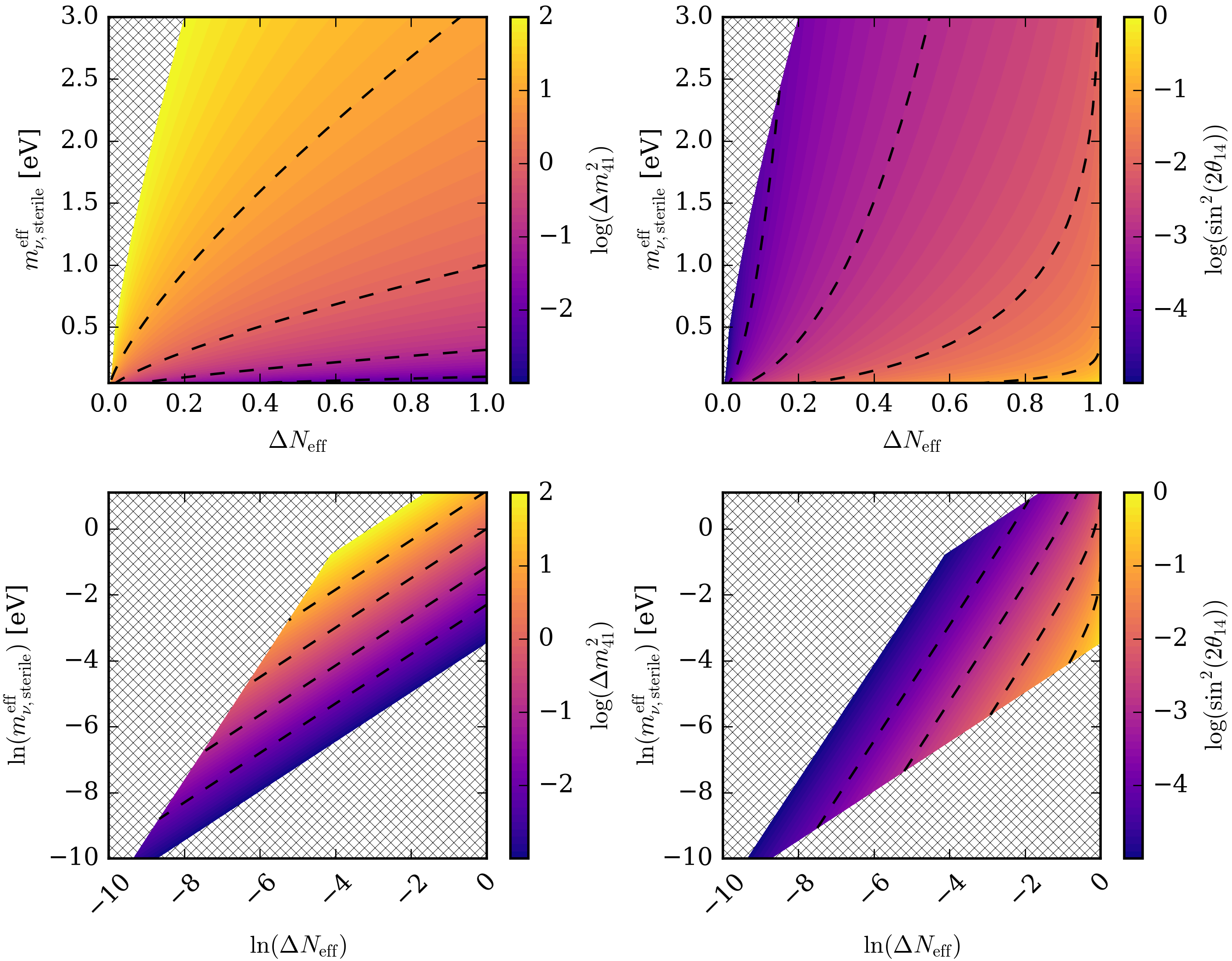
Since the particle parameters are not included in the base CosmoMC program, we instead vary $N_{\rm eff}$ and $m_{\nu,\rm sterile}^{\rm eff}$ and compute the particle parameters from the chains. To accomplish this, we follow the procedure described in ref. [16] to compute the cosmology parameters on a grid of values for $\Delta m_{41}^{2}$ and $\sin^{2}2\theta$ in the ranges

$$10^{-3}\leq\Delta m_{41}^{2}\leq 10^{2}\,\,\rm{eV}^{2},\quad 10^{-5}\leq\sin^{2}2\theta\leq 1.$$ (3.4)

The upper prior limit of 100 eV² for the mass splitting is consistent with setting an upper prior limit of $m_{4}<10$ eV on the physical sterile neutrino mass, as done in the Planck Collaboration analysis [9], which is chosen because at masses greater than 10 eV the sterile neutrinos begin to behave like cold dark matter and there is no need to handle them separately. For each point on the grid, we use the code LASAGNA [14] to compute $N_{\rm eff}$ and $m_{\nu,\rm sterile}^{\rm eff}$, yielding a mapping between the two parameter spaces. LASAGNA solves the quantum kinetic equations for sterile neutrino thermalization in the temperature range $1\leq T\leq 40$ MeV, generating discrete values of $x=p/T$ and $P_{\rm sterile}^{+}$, where $p$ is the neutrino momentum, $T$ is the temperature, and $P_{\rm sterile}^{+}$ is defined as

$$P_{\rm sterile}^{+}=(P_{0}+\bar{P_{0}})+(P_{z}+\bar{P_{z}}),$$ (3.5)

where $P_{i}$ are the elements of the quantum state vector ${\bf P}=(P_{0},P_{x},P_{y},P_{z})$ for a particular momentum mode. This output is used to evaluate the integral expression

$$\Delta N_{\rm eff}=N_{\rm eff}-3.046=\frac{\int dx\,x^{3}(1+e^{x})^{-1}P_{\rm sterile}^{+}}{4\int dx\,x^{3}(1+e^{x})^{-1}}$$ (3.6)

by summation. Refs. [14, 15] provide a detailed explanation of the formalism behind the LASAGNA code. To obtain an expression for $m_{\nu,\rm sterile}^{\rm eff}$, we assume thermally-distributed sterile neutrinos about some temperature $T_{\rm sterile}$ [16, 9]:

$$\Delta N_{\rm eff}=(T_{\rm sterile}/{T_{\nu}})^{4}.$$ (3.7)

When $T_{\nu}=T_{\rm sterile}$, the sterile neutrinos thermalize at the same temperature as the active neutrinos, resulting in full thermalization of the sterile neutrinos with $\Delta N_{\rm eff}=1$. The $T^{4}$ proportionality comes from the fact that $N_{\rm eff}$ is parameterizing an energy density. Matter densities, on the other hand, are proportional to $T^{3}$. Using $\Delta m_{41}^{2}=m_{4}^{2}$, we can compute $m_{\nu,\rm sterile}^{\rm eff}$ directly:

$$m_{\nu,\rm sterile}^{\rm eff} =(T_{\rm sterile}/{T_{\nu}})^{3}m_{4}^{\rm thermal}$$ (3.8)

$$=(\Delta N_{\rm eff})^{3/4}m_{4}^{\rm thermal}$$ (3.9)

$$=(\Delta N_{\rm eff})^{3/4}\sqrt{\Delta m_{41}^{2}}.$$ (3.10)

Figure 2: Left panel: Planck 68% and 95% CL constraints in the cosmology parameter space using Planck CMB TT+lowTEB data. Priors are flat in the ranges $3.046\leq N_{\rm eff}\leq 4.046$ and $0\leq m_{\nu,\rm sterile}^{\rm eff}\leq 3$ eV. Right panel: The procedure explained in section 3.2 is used to calculate the particle parameters from the original cosmology chains. The region of low mass and mixing angle appears to be ruled out, but these constraints are not robust, since this is a result of poor sampling. A solution to this is discussed in section 3.3. Note that here $\log x$ denotes the base 10 logarithm, not the natural logarithm, which we will always write as $\ln x$.

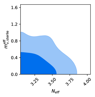
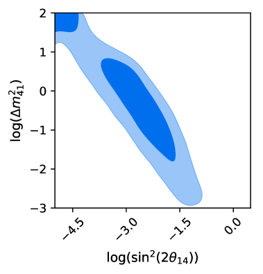
The LASAGNA calculations are quite sensitive to the initial lepton asymmetry $L$, which we take to be zero. The effects of varying this asymmetry have been studied previously [16], though for simplicity we do not consider it here. Such models may offer additional avenues for studying sterile neutrinos in cosmology. For example, it has been suggested that a large asymmetry could suppress the thermalization of sterile neutrinos in the early Universe, thereby allowing sterile neutrinos to have a large mixing angle without requiring $\Delta N_{\rm eff}\approx 1$, i.e. complete thermalization [15, 21, 22].

LASAGNA supports a single sterile neutrino species that mixes with one active neutrino species. The flavour of the active species can be either an electron neutrino or a muon neutrino, corresponding to the mixing angles $\theta_{14}$ and $\theta_{24}$, respectively [12]. We thus have two different cases, each parameterized by a different mixing angle. Both cases are considered in our MCMC runs, allowing us to obtain constraints on either $\sin^{2}2\theta_{14}$ or $\sin^{2}2\theta_{24}$.

3.3 Sampling

In order to avoid a false detection of sterile neutrinos, it is of critical importance to ensure that the region of parameter space corresponding to small mixing angles and mass splittings is well sampled. Indeed, if we simply compute the particle parameters from $N_{\rm eff}$ and $m_{\nu,\rm sterile}^{\rm eff}$, as was done in figure 2, the region of low mass and mixing angle appears to be ruled out at 95% confidence. However, this is not a genuine detection of high mass, but rather a consequence of the chains being unable to sample from this region. In figure 1, we can see that the region of particle space where both the mixing angle and mass splitting are small is where the darker regions overlap between the two panels. In the cosmology parameter space, there is practically no overlap at all and thus the Markov chain will be unable to sample this region. To remedy this we switch to a parameterization in terms of $\ln(\Delta N_{\rm eff})$ and $\ln(m_{\nu,\rm sterile}^{\rm eff})=\ln(\Omega_{\nu,\rm sterile}h^{2})+\ln(94.1)$. This effectively scales down the proposal width of the Markov chain when attempting to sample low $\sin^{2}2\theta$ and $\Delta m_{41}^{2}$, giving us much greater resolution at these small scales.

Figure 3: Left panel: Logarithmic values of the (non-normalized) Jacobian for the change of variables from the cosmology to particle parameter space, which gives flat priors in the linear particle space, for the case where the sterile neutrino mixes with an electron neutrino. Large negative values thus correspond to larger probabilities. The probability rises sharply at large $\ln(\Delta N_{\rm eff})$ and $\ln(m_{\nu,\rm sterile}^{\rm eff})$, indicated by the dark blue region in the upper right corner of the plot, and so this region is favoured by the prior. The hatched regions are excluded by the chosen prior ranges for the particle parameter space discussed in section 3.2. The priors for the two different mixing cases (i.e: muon or electron) are practically identical. Right panel: Logarithmic values of the Jacobian that gives flat priors in the log of the particle space (i.e. log priors). This prior favours lower masses and lepton numbers more than in the left panel, since log priors weigh each order of magnitude evenly.

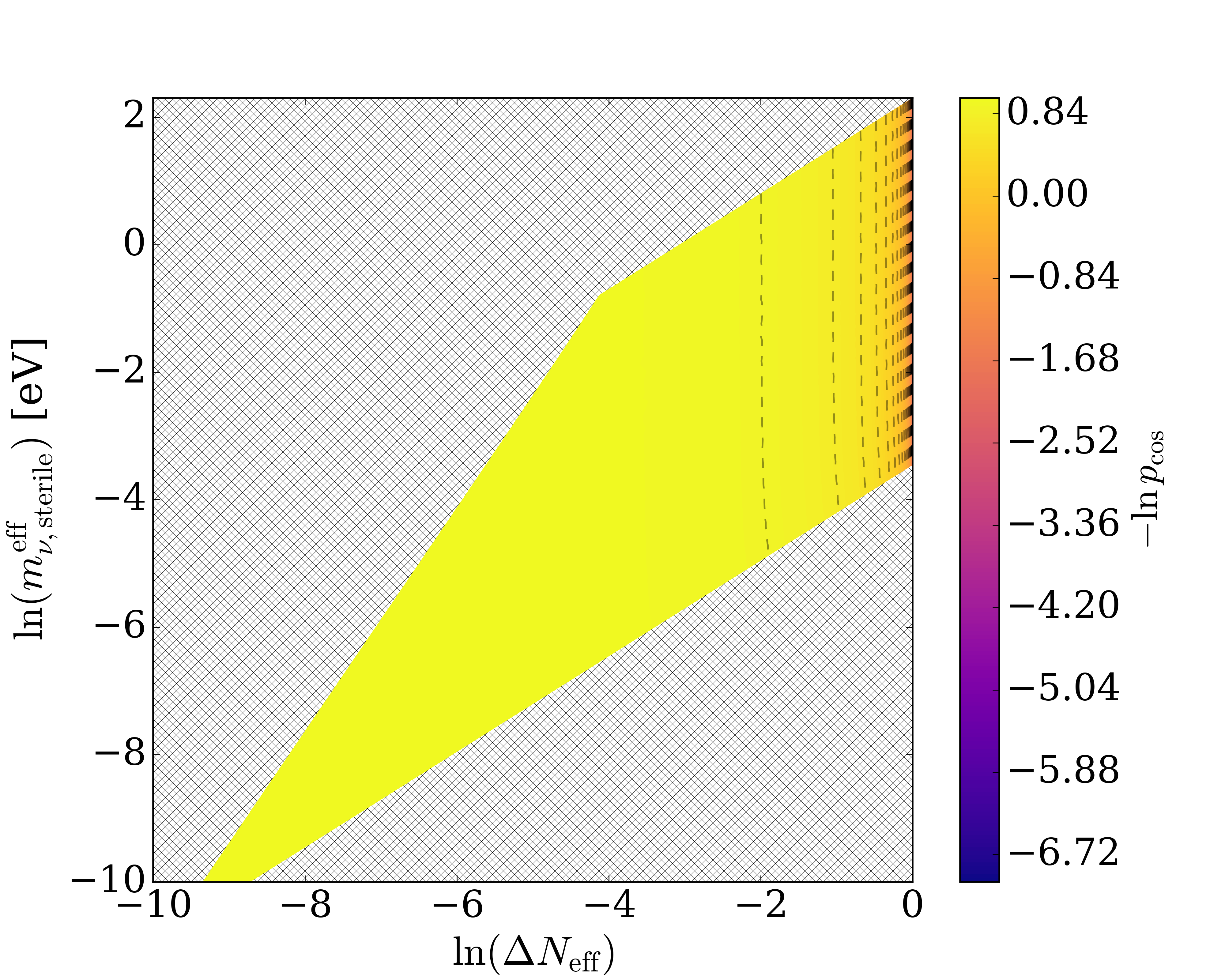
One can see in figure 1 that the overlapping region in the logarithmically-scaled plots is clearly visible and thus it should be well sampled when running the MCMC. The prior in this new parameter space that yields logarithmic priors in the particle space is

$$p_{\rm cos}\Big{(}\ln(\Delta N_{\rm eff}),\ln(m_{\nu,\rm sterile}^{\rm eff})\Big{)}\propto\biggl{|}\biggl{|}\frac{\partial(\log(\sin^{2}2\theta))\,\partial(\log(\Delta m_{41}^{2}))}{\partial(\ln(\Delta N_{\rm eff})\,\partial(\ln(m_{\nu,\rm sterile}^{\rm eff}))}\biggl{|}\biggl{|}.$$ (3.11)

We compute this Jacobian for each point in the cosmology parameter space by finding the partial derivatives numerically in each direction and then inverting the determinant of the resulting $2\times 2$ matrix:

$$\mathbb{J}=\begin{pmatrix}\dfrac{\partial(\ln(\Delta N_{\rm eff}))}{\partial(\log(\sin^{2}2\theta))}&&&\dfrac{\partial(\ln(\Delta N_{\rm eff}))}{\partial(\log(\Delta m_{41}^{2}))}\\ \dfrac{\partial(\ln(m_{\nu,\rm sterile}^{\rm eff}))}{\partial(\log(\sin^{2}2\theta))}&&&\dfrac{\partial(\ln(m_{\nu,\rm sterile}^{\rm eff}))}{\partial(\log(\Delta m_{41}^{2}))}\\ \end{pmatrix}.$$ (3.12)

The prior is implemented in CosmoMC by adding $-\ln p_{\rm cosm}$ to the negative log-likelihood function ($-\ln\mathcal{L}$) at each chain step, thereby changing the posteriors. We also introduce new prior ranges on the cosmology parameters,

$$-10\leq\ln(\Delta N_{\rm eff})\leq 0,\quad-10\leq\ln(m_{\nu,\rm sterile}^{\rm eff})\leq\ln{3}.$$ (3.13)

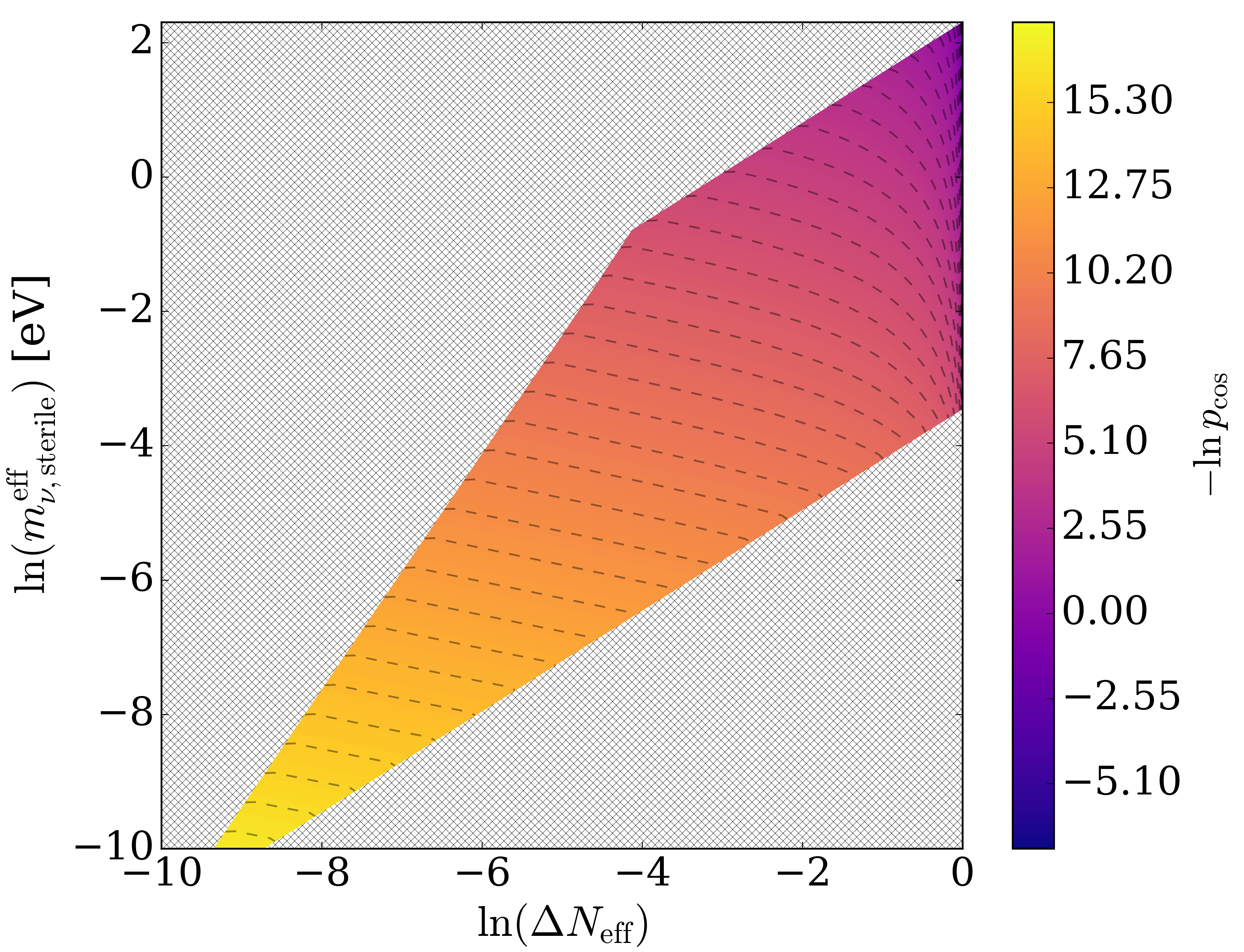
Since we have switched to logarithmic space, the baseline $\Lambda$CDM model with $\Delta N_{\rm eff}=0$ and $m_{\nu,\rm sterile}^{\rm eff}=0$ is formally excluded; however, the lower limit of $e^{-10}$ for both of these parameters is still very nearly standard $\Lambda$CDM. Since the default MCMC sampling method in CosmoMC is not well suited for dealing with priors with unusual distributions, we run CosmoChord alongside CosmoMC; this is a nested sampling tool designed to handle any arbitrarily complicated distribution [23, 24].

The Jacobians that give uniform and log priors in the particle space are shown in figure 3. The uniform prior on the particle parameters has the largest probabilities at high $N_{\rm eff}$. This is because, as noted in ref. [9], large mixing angles ($\sin^{2}2\theta\geq 0.1$) require near complete thermalization of sterile neutrinos, provided that there is no lepton asymmetry. A uniform prior on the mixing angle will hence favour $\Delta N_{\rm eff}\approx 1$. The sharp rise is less pronounced for log priors, owing to the fact that less weight is being placed on values of $\Delta N_{\rm eff}$ that are nearly unity.

3.4 Choosing a prior

Because these priors are quite different, they will have a significant effect on the final posteriors, and so it is very important to discuss the choice of prior. Log priors exclude values of zero for a parameter, since the log of that parameter goes out to negative infinity at zero. This is in contrast to uniform priors, where zero can be included within the prior ranges. If one uses log priors, then a non-zero lower prior limit must be chosen. This can be a source of confusion, since a value of zero is a priori excluded, which might lead one to mistakenly interpret a result using that prior as a genuine detection when it is really just a function of the choice of prior. Therefore, it is important to recognize that small non-zero posteriors at the lower limits of log priors is not indicative of a detection.

Since we want to present cosmological constraints on sterile neutrinos in a fashion that is easily comparable with constraints from particle physics experiments, we choose to implement logarithmic priors on the particle parameters in our analysis here. The mass-splitting is a scale parameter, and so the most appropriate uninformative prior in this case is one that weighs each order of magnitude uniformly, i.e. a logarithmic prior. Since $\theta$ is an angle parameter, one choice of an uninformative prior is uniform in $[0,2\pi]$. However, given that the quantity $\sin^{2}2\theta$ explicitly appears in the probability formula for neutrino oscillations, as shown in our earlier discussion in section 2, it is also reasonable to parameterize the mixing through this parameter. Furthermore, the use of log priors will tend to avoid biasing towards a detection, since log priors place more weight on smaller scales compared to uniform priors.

4 Results

To summarize our approach, we perform a Markov-chain Monte Carlo analysis using CosmoMC to sample the posteriors for a 2-parameter extension to the base-$\Lambda$CDM model,

$$\{\Omega_{\rm b}h^{2},\,\Omega_{\rm c}h^{2},\,100\theta_{\rm MC},\,\tau,\,\ln(10^{10}A_{\rm s}),\,n_{\rm s},\,\ln(\Delta N_{\rm eff}),\,\ln(m_{\nu,\rm sterile}^{\rm eff})\},$$ (4.1)

and we impose a Jacobian transformation for the prior on the cosmology parameters with the prior ranges in eq. 3.13, such that we have logarithmic priors in the particle parameter space in the ranges

$$10^{-3}\leq\Delta m_{41}^{2}\leq 10^{2}\,\,\rm{eV}^{2},\quad 10^{-5}\leq\sin^{2}2\theta\leq 1.$$ (4.2)

The standard $\Lambda$CDM parameters also have flat priors, as usual. The corresponding chains for the particle parameters are calculated from the cosmology parameters using eq. 3.10 and by interpolating over the grid for $\sin^{2}2\theta$. We also adopt the normal hierarchy, and assume that the SM neutrinos can be accurately approximated by a single massive species and two massless species, with $\Sigma m_{\nu}$ fixed at 0.06 eV. Two distinct mixing cases are considered: one where the sterile species mixes with an electron neutrino; and another where it mixes with a muon neutrino. We compare the results with MCMC runs that have flat priors in the cosmology space, as well as with the constraints from neutrino experiments. To be explicit, the data sets used in our MCMC analysis are:

TT+lowTEB power spectra – Planck 2015 high-$\ell$ ($30\leq\ell\leq 2508$) CMB temperature power spectrum combined with low-$\ell$ ($2\leq\ell\leq 29$) temperature and LFI polarization data, which uses the Plik likelihood code [25];
Lensing – Planck full-sky lensed CMB SMICA reconstruction [26];
BAO – baryon acoustic-oscillation data sets DR11CMASS, DR11LOWZ, 6DF, and MGS from the SDSS-III Baryon Oscillation Spectroscopic Survey (BOSS) [27].

4.1 Joint constraints on $\Delta m_{41}^{2}$ and $\sin^{2}2\theta_{14}$

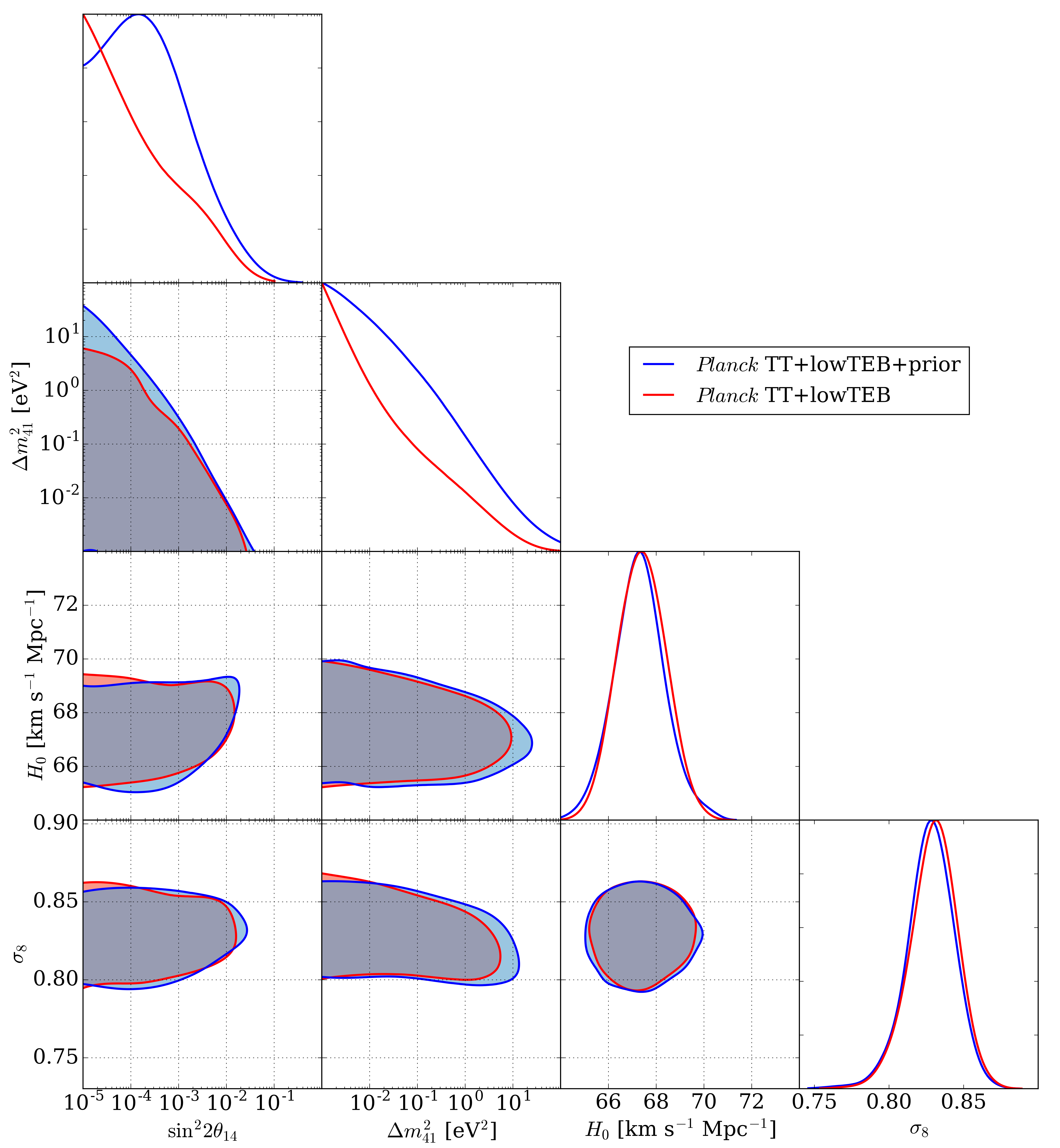
In this section we discuss the constraints from our MCMC analysis for the case where the sterile neutrino mixes with an electron neutrino. The top-left panel in figure LABEL:fig:planck_particle_14 shows the constraints in the particle space, with and without logarithmic priors in this space. With flat priors in the cosmology space, Planck data rule out large mass splittings and mixing angles at over 90% confidence. Furthermore, the posterior projections run up against the lower mass-splitting and mixing-angle limits, and are hence consistent with no sterile neutrinos. Furthermore, the region of low mixing angle and mass splitting is completely filled, demonstrating that this region of parameter space is being properly sampled by the MCMC.

Assuming flat priors in the particle parameter space changes the constraints noticeably. The TT+lowTEB constraints on the mass gives a modest change from the case of flat priors in the cosmology space; however, there is an increased preference for larger mixing angles. When CMB lensing and BAO data added, there is a slight preference for both larger mass-splittings and larger mixing angles. In particular, when all three data sets are used, the lower left region of the particle space is not completely filled by the 90% confidence contours. Low mixing angles are instead only favoured if the mass-splitting is above about 0.01 eV², and higher mixing angles are preferred if the mass is small. One might therefore interpret this as a possible hint of an intermediate-mass sterile neutrino with low mixing interactions with the SM neutrinos, or perhaps of a very light sterile neutrino with larger levels of mixing. The latter could be suggestive of a massless sterile neutrino, which has been considered in past cosmological studies, such as in ref. [28], in which the authors also claim to have found a hint of a massless sterile neutrino.

The 68% confidence limits for all relevant parameters are shown in table 1. Below we quote the 95% confidence limits on the particle parameters:

$$\left.\begin{aligned} \Delta m_{41}^{2}<5.9\,\,{\rm eV}^{2},\\ \sin^{2}2\theta_{14}<0.011,\end{aligned}\right\} {\rm 95\%\,\,TT+lowTEB+prior},$$ (4.3)

$$\left.\begin{aligned} \Delta m_{41}^{2}<2.6\,\,{\rm eV}^{2},\\ \sin^{2}2\theta_{14}<0.0089,\end{aligned}\right\} {\rm 95\%\,\,TT+lowTEB+lensing+prior},$$ (4.4)

$$\left.\begin{aligned} \Delta m_{41}^{2}\,\,{\rm unconstrained},\\ \sin^{2}2\theta_{14}<0.0068,\end{aligned}\right\} {\rm 95\%\,\,TT+lowTEB+lensing+BAO+prior.}$$ (4.5)

With logarithmic priors in the particle space, Planck TT+lowTEB power spectrum data yield upper bounds of $\Delta m_{41}^{2}<5.9$ eV² and $\sin^{2}2\theta_{14}<0.011$ at the 95% confidence level. CMB lensing brings the mixing angle constraint down to $\sin^{2}2\theta_{14}<0.0089$. The addition of CMB lensing and BAO further tightens the mixing angle constraint, but BAO weakens the constraint on the mass-splitting. In fact, BAO increases the likelihood at larger mass-splittings, compared to when BAO are not included, as seen by the posteriors in the right panel of figure LABEL:fig:planck_particle_14. However, we emphasize that the 1D posteriors presented in our analysis are still highly non-zero at the lower prior limits. As noted in our discussion of priors in section 3.4, the use of log priors technically means that zero mass-splitting and zero mixing are excluded by the prior ranges. In this case, non-zero posteriors at the lower limit of log priors are typically interpreted as plateaus that extend towards negative infinity. Our results here are therefore not indicative of any detection, and we conclude that the Planck data remain consistent with the scenario of no sterile neutrinos.

In figure LABEL:fig:planck_cosmo_14 we have shown the constraints on the cosmology space. With flat priors in the log-cosmology space, the posteriors run up against the lower prior edges, consistent with the grey contours in figure LABEL:fig:planck_cosmo_14. Switching to flat priors in the particle parameter space leads to slightly higher likelihoods for larger effective neutrino number and effective masses, and this is reflected in the particle constraints as increased likelihoods for higher mass-splittings. For TT+lowTEB+lensing+BAO, the 90% contours no longer run up against the lower prior limit, and so the apparent preference for higher mass-splittings is also visible in the cosmology parameters. This also provides a clearer picture of why BAO data weaken the constraint on the mass splitting. BAO lowers the likelihoods at low $\Delta N_{\rm eff}$ and $m_{\nu,\rm sterile}^{\rm eff}$, while increasing the likelihood at high $m_{\nu,\rm sterile}^{\rm eff}$, but leaving the mixing-angle posterior roughly the same as TT+lowTEB+lensing near the peak. This results in a better mixing-angle constraint, but a weaker mass-splitting constraint. The addition of lensing and BAO data to the Planck TT+lowTEB likelihood gives the highest value on the effective mass, and this is also where we see the highest upper bound on the mass splitting. These constraints nonetheless fall well within the $(N_{\rm eff},m_{\nu,\rm sterile}^{\rm eff})$ confidence limits of the Planck Collaboration analysis [9]. Fully thermalized sterile neutrinos with $\Delta N_{\rm eff}=1$ remain excluded at 90% confidence for all likelihood combinations. This suggests that any sterile neutrinos would have to be incompletely thermalized in the early Universe through some sort of cosmological suppression mechanism.

Parameter	TT+lowTEB+prior 68% limits	TT+lowTEB +lensing+prior                 68% limits	TT+lowTEB +lensing +BAO+prior                 68% limits
$\Omega_{\rm b}h^{2}$	$0.02221\pm 0.00024$	$0.02230\pm 0.00022$	$0.02229\pm 0.00020$
$\Omega_{\rm c}h^{2}$	$0.1203\pm 0.0023$	$0.1188\pm 0.0023$	$0.1183\pm 0.0017$
$100\theta_{\rm MC}$	$1.04081\pm 0.00047$	$1.04099\pm 0.00047$	$1.04097\pm 0.00041$
$\tau$	$0.084\pm 0.021$	$0.069\pm 0.016$	$0.068\pm 0.014$
$\ln(10^{10}A_{\rm s})$	$3.095\pm 0.035$	$3.069\pm 0.029$	$3.068\pm 0.026$
$n_{\rm s}$	$0.9654\pm 0.0068$	$0.9694\pm 0.0060$	$0.9687\pm 0.0051$
$\Delta N_{\rm eff}$	$0.010_{-0.0076}^{+0.069}$	$0.01_{-0.0091}^{+0.14}$	$0.01_{-0.0088}^{+0.10}$
$m_{\nu,\rm sterile}^{\rm eff}$ [eV]	$0.007_{-0.0057}^{+0.067}$	$0.008_{-0.0061}^{+0.084}$	$0.01_{-0.010}^{+0.13}$
$\Delta m_{41}^{2}$ [eV2]	$<0.14$	$<0.26$	$<0.41$
$\sin^{2}2\theta_{14}$	$0.00026_{-0.00025}^{+0.00098}$	$<0.0011$	$<0.00056$
$H_{0}$ [km s-1 Mpc-1]	$67.3\pm 1.1$	$68.00\pm 0.95$	$67.94\pm 0.61$
$\sigma_{8}$	$0.828\pm 0.016$	$0.812\pm 0.012$	$0.810\pm 0.015$

Table 1: 68% CL parameter constraints on the 2-parameter extension to the base-$\Lambda$CDM model for the electron-neutrino-mixing case, along with relevant derived parameters. The cosmology parameter constraints have been converted to linear values for ease of interpretation. Parameters with nearly Gaussian distributions are written with their mean and standard deviation, whereas non-Gaussian parameters have their mean and 68% limits quoted. For unconstrained parameters, only the 68% bounds are shown.

Figure 4: Covariances between the particle parameters, $H_{0}$, and $\sigma_{8}$ for the electron-neutrino mixing case. The solid blue lines are the results with flat priors in the particle space, and the dashed red lines are for flat priors in the log-cosmology space. The Planck TT+lowTEB data set is used here. Limits are at 90% confidence.

Because we have to explore the region of parameter space corresponding to very small $\Delta N_{\rm eff}$ and $m_{\nu,\rm sterile}^{\rm eff}$ down to the order of $10^{-5}$ to properly sample the particle parameters, LASAGNA enters scales at which it begins to encounter issues with accuracy. In the low mass-splitting region near $\Delta m_{41}^{2}\sim 10^{-3}\,{\rm eV}^{2}$, the error in $N_{\rm eff}$ is as large as 0.01 (see ref. [31] for a discussion of the accuracy of LASAGNA). Hence, the reader should note that the output of LASAGNA at the lower corner of the parameter space in figure LABEL:fig:planck_cosmo_14 is somewhat unreliable.

The Planck constraints are largely consistent with the neutrino disappearance searches shown in figure LABEL:fig:planck_particle_14. There is mild tension with Daya Bay+Bugey-3 at low mass-splitting, but given that these constraints are derived from completely different sets of data, some tension is to be expected. The cosmological constraints are much stronger than Daya Bay+Bugey-3 and LSND+KARMEN, excluding a much larger region of the parameter space. The recent detection of an excess of electron neutrino events by the MiniBooNE experiment has received a great deal of attention, and so we have also included these constraints in our plots. The MiniBooNE limits are in very strong tension with cosmology, as well as with various other particle physics experiments. The constraints from cosmology in particular completely rule out the regions allowed by MiniBooNE and LSND. However, we reiterate what we stated in section 2, that $\nu_{\mu}\rightarrow\nu_{e}$ appearance channels require a two-flavour oscillation model, and we have only constrained single flavour oscillation models, so these sets of constraints are not necessarily directly comparable.

Since a great deal of attention has been give to possible tensions between CMB measurements and several low-redshift parameter constraints [32], it is worth examining how sterile neutrinos might affect these tensions. In figure 4 we have plotted the covariances between the particle parameters and the linear power spectrum amplitude $\sigma_{8}$, and the Hubble parameter $H_{0}$. Increasing the mixing angle or the mass-splitting has no significant affect on the value of $\sigma_{8}$. Larger mixing angles lead to marginal increases in the value of $H_{0}$, and so high sterile-neutrino mixing may provide a path towards resolving the $H_{0}$ tensions. There is little correlation between the mass-splitting and $H_{0}$, but increasing the mass does appear to lower $\sigma_{8}$ slightly. The switch to log priors does not affect the distributions of $\sigma_{8}$ and $H_{0}$ significantly either.

In our earlier discussion of priors, we noted that a log prior must have a non-zero lower limit. It therefore seems plausible that constraints derived with such priors may be sensitive to the choice of this lower limit, and in the case of sterile neutrinos, choosing too high of a lower limit could mask potential signatures of a detection. We ran additional MCMC chains using a lower limit on the mass splitting of $10^{-5}$ eV² to check the robustness of our constraints, finding no significant differences that would affect our overall conclusions.

4.2 Joint constraints on $\Delta m_{41}^{2}$ and $\sin^{2}2\theta_{24}$

Having the sterile neutrino mix with a muon neutrino, as opposed to an electron neutrino, makes very little difference to the calculation of $\Delta N_{\rm eff}$ and $m_{\nu,\rm sterile}^{\rm eff}$. The constraint on $\sin^{2}2\theta_{24}$ will be very similar to the constraint on $\sin^{2}2\theta_{14}$, and thus most of what has been said about the latter will be applicable to the former. Since the Jacobians for the two cases are quite similar, the ratio of the Jacobians is approximately constant, and so we can obtain the corresponding posteriors for the muon neutrino mixing case by multiplying the likelihoods from the previous set of chains by this ratio.

Figure 5: Left panel: Joint constraints on the particle parameters for the muon-neutrino mixing case, for the two sets of priors. The shaded regions represent the 90% confidence limits unless otherwise stated. The colour scheme is the same as in figure LABEL:fig:planck_particle_14. Note that in the legend, “prior” denotes logarithmic priors in the particle space. Right panels: One-dimensional posteriors for the particle parameters from our analysis of Planck data. The line style and colour coding follows the same scheme as in the left panel.

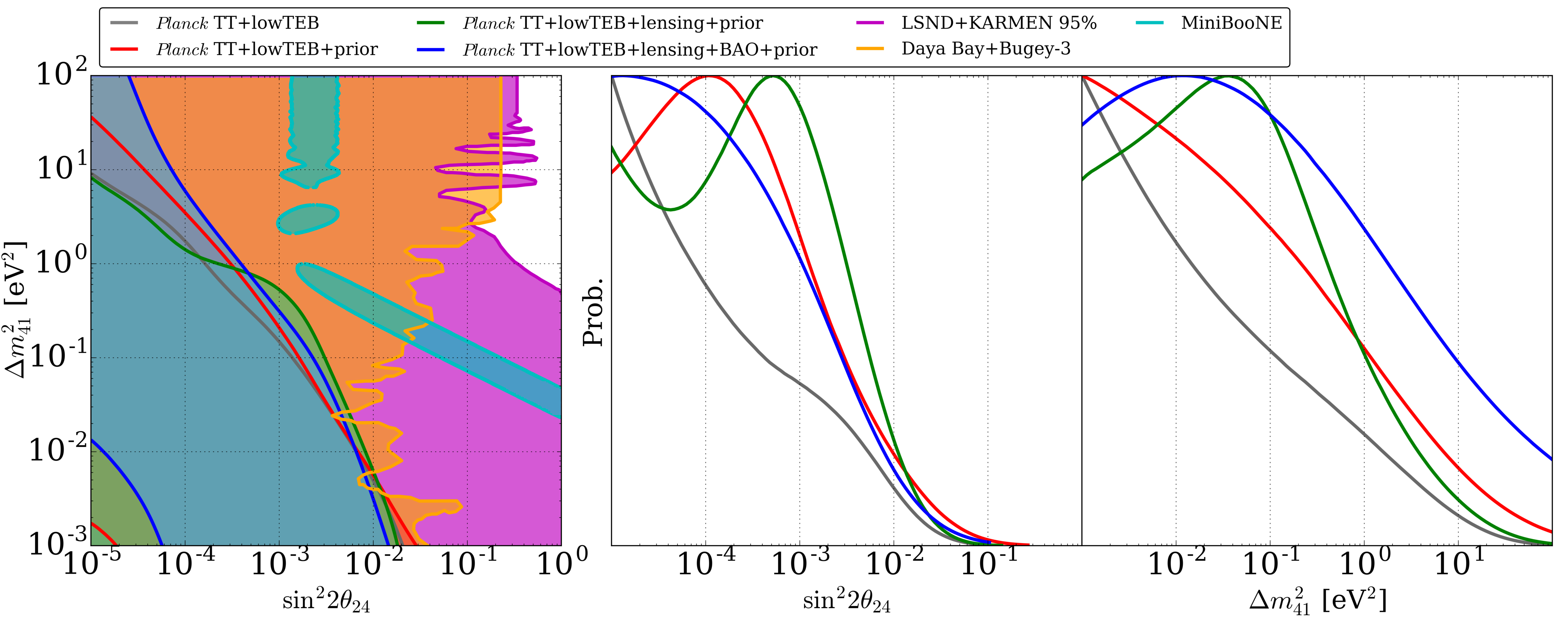
The 95% limits for the particle parameters for the muon neutrino mixing case are:

$$\left.\begin{aligned} \Delta m_{41}^{2}<5.1\,\,{\rm eV}^{2},\\ \sin^{2}2\theta_{24}<0.0088,\end{aligned}\right\} {\rm 95\%\,\,TT+lowTEB+prior};$$ (4.6)

$$\left.\begin{aligned} \Delta m_{41}^{2}<2.4\,\,{\rm eV}^{2},\\ \sin^{2}2\theta_{24}<0.0067,\end{aligned}\right\} {\rm 95\%\,\,TT+lowTEB+lensing+prior};$$ (4.7)

$$\left.\begin{aligned} \Delta m_{41}^{2}\,\,{\rm unconstrained},\\ \sin^{2}2\theta_{24}<0.0052,\end{aligned}\right\} {\rm 95\%\,\,TT+lowTEB+lensing+BAO+prior};$$ (4.8)

and the contours are plotted in figure 5.

5 Forecasting

Several future CMB experiments, like CMB-S4 [33, 34], aim to improve the sensitivity to cosmological neutrinos, and therefore find more stringent constraints on sterile neutrinos than Planck. Fisher-matrix methods are commonly used by cosmologists to predict the precision with which these future experiments could measure cosmological parameters, and in this section we proceed to apply these techniques to forecast sterile neutrino constraints in the particle parameter space.

5.1 The CMB Fisher matrix

To forecast constraints from the CMB, one must first calculate the Fisher matrix for a given fiducial (baseline) model. For an $n$-parameter model, the Fisher matrix is a square $n\times n$ matrix that fully encodes all the information from the CMB. Calculating Fisher matrices normally involves finding the first moment of the Hessian of the log-likelihood function for the fiducial model. However, by assuming Gaussian perturbations in the CMB temperature and polarization anisotropies, the Fisher matrix for the CMB can be rewritten as [35]

$$F_{ij}=\sum_{\ell}\sum_{XY}\dfrac{\partial C_{\ell}^{X}}{\partial p_{i}}(\mathbb{C})_{XY}^{-1}\dfrac{\partial C_{\ell}^{Y}}{\partial p_{j}}$$ (5.1)

where $X=T,E,C$, respectively, denote the temperature, $E$-mode polarization, and temperature-polarization cross-correlation terms, $p_{i}$ are the model parameters, and $\mathbb{C}$ is the CMB covariance matrix

$$\mathbb{C}=\begin{pmatrix}(\mathbb{C})_{TT}&&(\mathbb{C})_{TE}&&(\mathbb{C})_{TC}\\ (\mathbb{C})_{TE}&&(\mathbb{C})_{EE}&&(\mathbb{C})_{EC}\\ (\mathbb{C})_{TC}&&(\mathbb{C})_{EC}&&(\mathbb{C})_{CC}\end{pmatrix}.$$ (5.2)

Here we have ignored the primordial $B$-modes, since they are yet to be well measured and are likely far too weak for our model to be sensitive to them [36]. The Cramer-Rao inequality then places upper bounds on the errors for the model parameters, $\sigma_{i}\leq\sqrt{F_{ii}^{-1}}$. The inverse of the Fisher matrix is used, since all the model parameters are allowed to float. If one does not use the inverse here, then the errors correspond to the case where all the other parameters are fixed. The derivatives of the $C_{\ell}$s in eq. 5.1 are taken about the chosen fiducial model.

Accounting for instrumental noise, the elements of the covariance matrix are [35]

$$(\mathbb{C})_{TT} =\frac{2}{(2\ell+1)f_{\rm sky}}(C_{\ell}^{TT}+w_{T}^{-1}B_{\ell}^{-2})^{2},$$ (5.3)

$$(\mathbb{C})_{TE} =\frac{2}{(2\ell+1)f_{\rm sky}}(C_{\ell}^{TE})^{2},$$ (5.4)

$$(\mathbb{C})_{TC} =\frac{2}{(2\ell+1)f_{\rm sky}}C_{\ell}^{TE}(C_{\ell}^{TT}+w_{T}^{-1}B_{\ell}^{-2}),$$ (5.5)

$$(\mathbb{C})_{EE} =\frac{2}{(2\ell+1)f_{\rm sky}}(C_{\ell}^{EE}+w_{P}^{-1}B_{\ell}^{-2})^{2},$$ (5.6)

$$(\mathbb{C})_{EC} =\frac{2}{(2\ell+1)f_{\rm sky}}C_{\ell}^{TE}(C_{\ell}^{EE}+w_{P}^{-1}B_{\ell}^{-2}),$$ (5.7)

$$(\mathbb{C})_{CC} =\frac{1}{(2\ell+1)f_{\rm sky}}[(C_{\ell}^{TE})^{2}+(C_{\ell}^{TT}+w_{T}^{-1}B_{\ell}^{-2})(C_{\ell}^{EE}+w_{P}^{-1}B_{\ell}^{-2})],$$ (5.8)

The constants $w_{T}$ and $w_{P}$ are the inverse squares of the detector noise level over a steradian patch of the sky for $T$ and $E$, $f_{\rm sky}$ is the fraction of the sky being observed, and

$$B_{\ell}^{2}=\exp\bigg{(}\frac{-\ell(\ell+1)\theta_{\rm beam}^{2}}{8\ln 2}\bigg{)}$$ (5.9)

is the beam window function, where $\theta_{\rm beam}$ is the full-width, half-maximum beam angle [35]. The noise terms vanish in the limit of zero detector noise, $w_{T},w_{P}\rightarrow\infty$, yielding the covariance matrix for the noise-free case. The elements of the Fisher matrix encode the confidence ellipses for every pair of parameters, marginalized over all other parameters. Given two parameters $x$ and $y$, with $1\sigma$ Fisher uncertainties $\sigma_{x}$ and $\sigma_{y}$, and with correlation cross-terms $\sigma_{xy}=\sigma_{yx}$, the ellipse axis parameters are calculated as [37]

$$a^{2}=\frac{\sigma_{x}^{2}+\sigma_{y}^{2}}{2}+\sqrt{\frac{(\sigma_{x}^{2}-\sigma_{y}^{2})^{2}}{4}+\sigma_{xy}^{2}},$$ (5.10)

$$b^{2}=\frac{\sigma_{x}^{2}+\sigma_{y}^{2}}{2}-\sqrt{\frac{(\sigma_{x}^{2}-\sigma_{y}^{2})^{2}}{4}+\sigma_{xy}^{2}},$$ (5.11)

where $a$ corresponds to the semimajor axis, and $b$ to the semiminor axis. The angle that controls the (counterclockwise) tilt of the ellipse is given by [37]

$$\tan 2\theta=\frac{2\sigma_{xy}}{\sigma_{x}^{2}-\sigma_{y}^{2}}.$$ (5.12)

Figure 6: Fisher confidence ellipses in the particle space for an experiment resembling CMB-S4, with $f_{\rm sky}=0.4$, a 1-arcmin beam, and noise levels in $T$ and $E$ of $1\,\mu$K-arcmin and $\sqrt{2}\,\mu$K-arcmin, respectively [33]. The covariance matrix for the full $TT+TE+EE$ spectrum is used. The fiducial model is the best-fit TT+lowTEB point, $(\Delta m_{41}^{2},\sin^{2}2\theta_{14})=(0.0038\,\,{\rm eV}^{2},0.00013)$. The contours are drawn at 68%, 90%, and 95% confidence. For comparison, we have included the LSND+KARMEN 95%, Daya Bay+Bugey-3 90%, and MiniBooNE 90% constraints previously shown in figures LABEL:fig:planck_particle_14 and 5. Note that the regions to the right of the orange and magenta curves are excluded.

5.2 Particle parameter forecasts

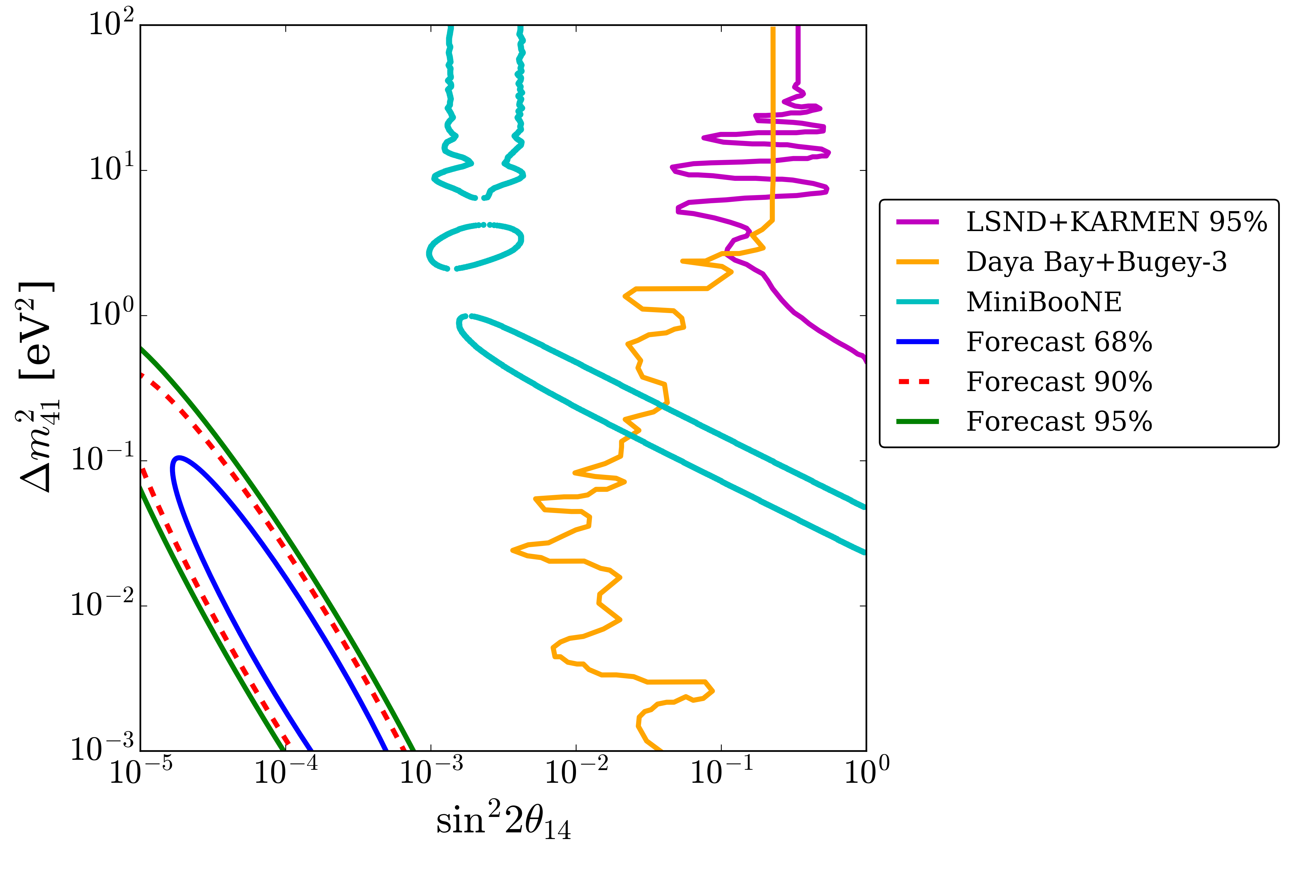
We use CAMB [20] to compute the power spectra in order to find the derivatives of the $C_{\ell}$s with respect to each parameter for the 2-parameter extension to the $\Lambda$CDM presented in section 4. The derivatives with respect to the log of the particle parameters are computed from the derivatives with respect to $\ln(\Delta N_{\rm eff})$ and $\ln(m_{\nu,\rm sterile}^{\rm eff})$ and then applying the chain rule. We then calculate the Fisher matrix for an experiment with noise levels and beam settings similar to those of CMB-S4, using the full $TT+TE+EE$ covariance matrix, which we then invert to find the uncertainties. The fiducial model is the best-fit (maximum likelihood) point from the TT+lowTEB MCMC run, $(\Delta m_{41}^{2},\sin^{2}2\theta_{14})=(0.0038\,\,{\rm eV}^{2},0.00013)$. The confidence ellipses are plotted in figure 6. The $1\sigma$ errors on the particle parameters, in log space, are

$$\sigma(\log(\Delta m_{41}^{2}))=0.95\,\,{\rm eV}^{2},\quad\sigma(\log(\sin^{2}2\theta_{14}))=0.58,$$ (5.13)

and represent close to the best possible measurement on these parameters obtainable using the CMB. Figure 6 shows that this best possible CMB constraint is significantly better than what current Planck data can do, and remains competitive with particle physics experiments. Therefore, future CMB experiments will still be of great importance with regards to further constraining sterile neutrinos, and will potentially show whether any of the hints of sterile neutrinos encountered thus far turn out to be signs of new physics or not.

6 Conclusions

We have used Planck data to obtain cosmological constraints on the sterile-neutrino oscillation parameters: the squared mass splitting $\Delta m_{41}^{2}$; and the mixing angles $\sin^{2}2\theta_{14}$ and $\sin^{2}2\theta_{24}$, corresponding to two different models where a single sterile neutrino species mixes with an electron neutrino or a muon neutrino. The posteriors were inferred using an MCMC analysis of Planck CMB power spectra, lensing, and BAO data, where our model consists of the six $\Lambda$CDM parameters plus $\ln(\Delta N_{\rm eff})$ and $\ln(m_{\nu,\rm sterile}^{\rm eff})$, which were used to vary $\Delta m_{41}^{2}$ and $\sin^{2}2\theta$ by proxy. We compared results that have flat priors in the cosmology space with results that had logarithmic priors in the particle parameter space, which was accomplished by imposing the Jacobian of the change of variables transformation between the two parameter spaces as the prior on the cosmology space. The Planck data show slightly increased preference for non-zero mass-splitting when priors are flat in the particle space in the range $10^{-3}\leq\Delta m_{41}^{2}\leq 10^{2}$ eV², $10^{-5}\leq\sin^{2}2\theta\leq 1$. For the model where the sterile neutrino mixes with an electron neutrino, we find constraints of $\Delta m_{41}^{2}<0.41$ eV² and $\sin^{2}2\theta_{14}<0.00056$ at 68% confidence for the TT+lowTEB+lensing+BAO likelihoods. At 95% confidence, the mixing angle constraint increases to $\sin^{2}2\theta_{14}<0.0068$, and the probabilities for higher values of $\Delta m_{41}^{2}$ also increase, but the data are unable to constrain the mass splitting at this confidence level. For the second case where the sterile neutrino mixes with a muon neutrino, we find that $\Delta m_{41}^{2}$ is again unconstrained and $\sin^{2}2\theta_{24}<0.0052$ at 95% confidence, using all three data sets. In summary, we conclude that the Planck data indicate no evidence for sterile neutrinos. We have also compared these results with sterile neutrino constraints from particle physics experiments, and have shown that cosmology strongly rules out the region of particle space allowed by LSND and MiniBooNE. However, our analysis has assumed that sterile neutrinos mix with a single neutrino flavour, and so the assumptions made here are not exactly the same as those used by LSND and MiniBooNE.

The search for sterile neutrinos is certainly not over. The anomalies observed in LSND and MiniBooNE remain unexplained, and future particle physics experiments will no doubt attempt to hone in on the culprit, be it sterile neutrinos or something else. Future cosmology experiments also promise to find more stringent constraints on cosmological neutrinos, and will likely elaborate more on the status of sterile neutrinos within cosmology.

References

- [1] Particle Data Group collaboration, M. Tanabashi et al., Review of Particle Physics, Phys. Rev. D98 (2018) 030001.
- [2] K. N. Abazajian et al., Light Sterile Neutrinos: A White Paper, 1204.5379.
- [3] LSND collaboration, A. Aguilar-Arevalo et al., Evidence for neutrino oscillations from the observation of anti-neutrino(electron) appearance in a anti-neutrino(muon) beam, Phys. Rev. D64 (2001) 112007 [hep-ex/0104049].
- [4] OPERA collaboration, N. Agafonova et al., Final results of the search for oscillations with the OPERA detector in the CNGS beam, JHEP 06 (2018) 151 [1803.11400].
- [5] MiniBooNE collaboration, A. A. Aguilar-Arevalo et al., Significant Excess of ElectronLike Events in the MiniBooNE Short-Baseline Neutrino Experiment, 1805.12028.
- [6] G. Mangano, G. Miele, S. Pastor and M. Peloso, A Precision calculation of the effective number of cosmological neutrinos, Phys. Lett. B534 (2002) 8 [astro-ph/0111408].
- [7] G. Mangano, G. Miele, S. Pastor, T. Pinto, O. Pisanti and P. D. Serpico, Relic neutrino decoupling including flavour oscillations, Nuclear Physics B 729 (2005) 221 [hep-ph/0506164].
- [8] P. F. de Salas and S. Pastor, Relic neutrino decoupling with flavour oscillations revisited, JCAP 1607 (2016) 051 [1606.06986].
- [9] Planck collaboration, Planck 2015 results. XIII. Cosmological parameters, Astron. Astrophys. 594 (2016) A13 [1502.01589].
- [10] J. Lesgourgues and S. Pastor, Massive neutrinos and cosmology, Phys. Rept. 429 (2006) 307 [astro-ph/0603494].
- [11] A. Lewis, “CAMB Notes.” https://cosmologist.info/notes/CAMB.pdf, 2014.
- [12] J. Kopp, P. A. N. Machado, M. Maltoni and T. Schwetz, Sterile Neutrino Oscillations: The Global Picture, JHEP 05 (2013) 050 [1303.3011].
- [13] V. Barger, D. Marfatia and K. Whisnant, The Physics of Neutrinos. Princeton University Press, 2012.
- [14] S. Hannestad, R. S. Hansen and T. Tram, Can active-sterile neutrino oscillations lead to chaotic behavior of the cosmological lepton asymmetry?, JCAP 1304 (2013) 032 [1302.7279].
- [15] S. Hannestad, I. Tamborra and T. Tram, Thermalisation of light sterile neutrinos in the early universe, JCAP 1207 (2012) 025 [1204.5861].
- [16] S. Bridle, J. Elvin-Poole, J. Evans, S. Fernandez, P. Guzowski and S. Soldner-Rembold, A Combined View of Sterile-Neutrino Constraints from CMB and Neutrino Oscillation Measurements, Phys. Lett. B764 (2017) 322 [1607.00032].
- [17] A. Lewis, Efficient sampling of fast and slow cosmological parameters, Phys. Rev. D87 (2013) 103529 [1304.4473].
- [18] A. Lewis and S. Bridle, Cosmological parameters from CMB and other data: A Monte Carlo approach, Phys. Rev. D66 (2002) 103511 [astro-ph/0205436].
- [19] P. C. Gregory, Bayesian Logical Data Analysis for the Physical Sciences. Cambridge University Press, 2005.
- [20] A. Lewis, A. Challinor and A. Lasenby, Efficient computation of CMB anisotropies in closed FRW models, Astrophys. J. 538 (2000) 473 [astro-ph/9911177].
- [21] N. Saviano, A. Mirizzi, O. Pisanti, P. D. Serpico, G. Mangano and G. Miele, Multi-momentum and multi-flavour active-sterile neutrino oscillations in the early universe: role of neutrino asymmetries and effects on nucleosynthesis, Phys. Rev. D87 (2013) 073006 [1302.1200].
- [22] S. Gariazzo, C. Giunti and M. Laveder, Cosmological Invisible Decay of Light Sterile Neutrinos, 1404.6160.
- [23] W. J. Handley, M. P. Hobson and A. N. Lasenby, PolyChord: nested sampling for cosmology, Mon. Not. Roy. Astron. Soc. 450 (2015) L61 [1502.01856].
- [24] W. J. Handley, M. P. Hobson and A. N. Lasenby, POLYCHORD: next-generation nested sampling, Mon. Not. Roy. Astron. Soc. 453 (2015) 4384 [1506.00171].
- [25] Planck collaboration, Planck 2015 results. XI. CMB power spectra, likelihoods, and robustness of parameters, Astron. Astrophys. 594 (2016) A11 [1507.02704].
- [26] Planck collaboration, P. A. R. Ade et al., Planck 2015 results. XV. Gravitational lensing, Astron. Astrophys. 594 (2016) A15 [1502.01591].
- [27] BOSS collaboration, L. Anderson et al., The clustering of galaxies in the SDSS-III Baryon Oscillation Spectroscopic Survey: baryon acoustic oscillations in the Data Releases 10 and 11 Galaxy samples, Mon. Not. Roy. Astron. Soc. 441 (2014) 24 [1312.4877].
- [28] L. Feng, J.-F. Zhang and X. Zhang, A search for sterile neutrinos with the latest cosmological observations, Eur. Phys. J. C77 (2017) 418 [1703.04884].
- [29] J. M. Conrad and M. H. Shaevitz, Limits on Electron Neutrino Disappearance from the KARMEN and LSND - Carbon Cross Section Data, Phys. Rev. D85 (2012) 013017 [1106.5552].
- [30] MINOS, Daya Bay collaboration, P. Adamson et al., Limits on Active to Sterile Neutrino Oscillations from Disappearance Searches in the MINOS, Daya Bay, and Bugey-3 Experiments, Phys. Rev. Lett. 117 (2016) 151801 [1607.01177].
- [31] S. Hannestad, R. S. Hansen, T. Tram and Y. Y. Y. Wong, Active-sterile neutrino oscillations in the early Universe with full collision terms, JCAP 1508 (2015) 019 [1506.05266].
- [32] A. G. Riess et al., A 2.4% Determination of the Local Value of the Hubble Constant, Astrophys. J. 826 (2016) 56 [1604.01424].
- [33] CMB-S4 collaboration, K. N. Abazajian et al., CMB-S4 Science Book, First Edition, 1610.02743.
- [34] M. H. Abitbol, Z. Ahmed, D. Barron, R. Basu Thakur, A. N. Bender, B. A. Benson et al., CMB-S4 Technology Book, First Edition, ArXiv e-prints (2017) [1706.02464].
- [35] D. J. Eisenstein, W. Hu and M. Tegmark, Cosmic complementarity: Joint parameter estimation from CMB experiments and redshift surveys, Astrophys. J. 518 (1999) 2 [astro-ph/9807130].
- [36] D. Scott, D. Contreras, A. Narimani and Y.-Z. Ma, The information content of cosmic microwave background anisotropies, JCAP 1606 (2016) 046 [1603.03550].
- [37] D. Coe, Fisher Matrices and Confidence Ellipses: A Quick-Start Guide and Software, (2009) [0906.4123].