Low-Complexity Data-Parallel Earth Mover’s Distance Approximations

Abstract

The Earth Mover’s Distance (EMD) is a state-of-the art metric for comparing discrete probability distributions, but its high distinguishability comes at a high cost in computational complexity. Even though linear-complexity approximation algorithms have been proposed to improve its scalability, these algorithms are either limited to vector spaces with only a few dimensions or they become ineffective when the degree of overlap between the probability distributions is high. We propose novel approximation algorithms that overcome both of these limitations, yet still achieve linear time complexity. All our algorithms are data parallel, and thus, we take advantage of massively parallel computing engines, such as Graphics Processing Units (GPUs). On the popular text-based 20 Newsgroups dataset, the new algorithms are four orders of magnitude faster than a multi-threaded CPU implementation of Word Mover’s Distance and match its nearest-neighbors-search accuracy. On MNIST images, the new algorithms are four orders of magnitude faster than a GPU implementation of the Sinkhorn’s algorithm while offering a slightly higher nearest-neighbors-search accuracy.

1 Introduction

Earth Mover’s Distance (EMD) was initially proposed in the image retrieval field to quantify the similarity between images (rubnertg98). In the optimization theory, a more general formulation of EMD, called Wasserstein distance, has been used extensively to measure the distance between probability distributions (villani2003). In statistics, an equivalent measure is known as Mallows distance (emd_mallows). This paper uses the EMD measure for similary search in image and text databases.

In the text retrieval domain, an adaptation of EMD, called Word Mover’s Distance (WMD), has emerged as a state-of-the-art semantic similarity metric (kusnerskw15). WMD captures semantic similarity by using the concept of word embeddings in the computation of EMD. Word embeddings map words into a high-dimensional vector space such that the words that are semantically similar are close to each other. These vectors can be pre-trained in an unsupervised way, e.g., by running the Word2vec algorithm (mikolovcorr2013) on publicly available data sets. The net effect is that, given two sentences that cover the same topic, but have no words in common, traditional methods, such as cosine similarity, fail to detect the similarity. However, WMD detects and quantifies the similarity by taking the proximity between different words into account.

What makes EMD-based approaches attractive is their high search and classification accuracy. However, such an accuracy does not come for free. In general, the time complexity of computing these measures grows cubically in the size of the input probability distributions. Such a high complexity renders their use impractical for large datasets. Thus, there is a need for low-complexity approximation methods.

EMD can be computed in quadratic time complexity when an $L_{1}$ ground distance is used (Ling2007; Gudmundsson07). In addition, approximations of EMD can be computed in linear time by embedding EMD into Euclidean space (Indyk2003). However, such embeddings result in high distortions in high-dimensional spaces (Naor2006). An algorithm for computing EMD in the wavelet domain has also been proposed (ShirdhonkarJ08), which achieves linear time complexity in the size of the input distributions. However, the complexity grows exponentially in the dimensionality of the underlying vector space. Thus, both linear-complexity approaches are impractical when the number of dimensions is more than three or four. For instance, they are not applicable to WMD because the word vectors typically have several hundred dimensions.

A linear-complexity algorithm for computing approximate EMD distances over high-dimensional vector spaces has also been proposed (AtasuBigData17). The algorithm, called Linear-Complexity Relaxed Word Mover’s Distance (LC-RWMD), achieves four orders of magnitude improvement in speed with respect to WMD. In addition, on compact and curated text documents, it computes high-quality search results that are comparable to those found by WMD. Despite its scalability, the limitations of LC-RWMD are not well understood. Our analysis shows that 1) it is not applicable to dense histograms, and 2) its accuracy decreases when comparing probability distributions with many overlapping coordinates. Our main contributions are as follows:

• We propose new distance measures that are more robust and provably more accurate than LC-RWMD.

• We show that the new measures effectively quantify the similarity between dense as well as overlapping probability distributions, e.g., greyscale images.

• We show that the new measures can be computed in linear time complexity in the size of the input probability distributions: the same as for LC-RWMD.

• We propose data-parallel algorithms that achieve four orders of magnitude speed-up with respect to state of the art without giving up any search accuracy.

2 Background

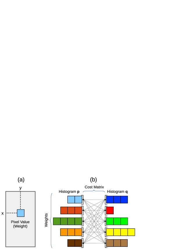
EMD can be considered as the discrete version of the Wasserstein distance, and can be used to quantify the affinity between discrete probability distributions. Each probability distribution is modelled as a histogram, wherein each bin is associated with a weight and a coordinate in a multi-dimensional vector space. For instance, when measuring the distance between greyscale images, the histogram weights are given by the pixel values and the coordinates are defined by the respective pixel positions (see Fig. 1 (a)).

The distance between two histograms is calculated as the cost of transforming one into the other. Transforming a first histogram into a second one involves moving weights from the bins of the first histogram into the bins of the second, thereby constructing the second histogram from the first. The goal is to minimize the total distance travelled, wherein the pairwise distances between different histogram bins are computed based on their respective coordinates. This optimization problem is well studied in transportation theory and is the discrete formulation of the Wasserstein distance.

Figure 1: (a) Converting a 28x28 image into a histogram with $h$=28x28=784 bins. The weights are the pixel values and the embedding vectors are the pixel coordinates. (b) Computing the EMD between two flattened histograms for an $h$x$h$ cost matrix $\mathbf{C}$.

Assume that histograms $\mathbf{p}$ and $\mathbf{q}$ are being compared, where $\mathbf{p}$ has $h_{p}$ entries and $\mathbf{q}$ has $h_{q}$ entries. Assume also that an $h_{p}\times h_{q}$ nonnegative cost matrix $\mathbf{C}$ is available. Note that ${p}_{i}$ indicates the weight stored in the $i$th bin of histogram $\mathbf{p}$, ${q}_{j}$ the weight stored in the $j$th bin of histogram $\mathbf{q}$, and ${C}_{i,j}$ the distance between the coordinates of the $i$th bin of $\mathbf{p}$ and the $j$th bin of $\mathbf{q}$ (see Fig. 1 (b)). Suppose that the histograms are $L_{1}$-normalized: $\sum_{i}{p}_{i}=\sum_{j}{q}_{j}=1$.

We would like to discover a non-negative flow matrix $\mathbf{F}$, where ${F}_{i,j}$ indicates how much of the bin $i$ of $\mathbf{p}$ has to flow to the bin $j$ of $\mathbf{q}$, such that the cost of moving $\mathbf{p}$ into $\mathbf{q}$ is minimized. Formally, the objective of EMD is as follows:

$$\text{EMD}(\mathbf{p},\mathbf{q})=\min_{{F}_{i,j}\geq 0}\sum_{i,j}{F}_{i,j}\cdot{C}_{i,j}.$$ (1)

A valid solution to EMD has to satisfy the so-called out-flow (2) and in-flow (3) constraints. The out-flow constraints ensure that, for each $i$ of $\mathbf{p}$, the sum of all the flows exiting $i$ is equal to ${p}_{i}$. The in-flow constraints ensure that, for each $j$ of $\mathbf{q}$, the sum of all the flows entering $j$ is equal to ${q}_{j}$. These constraints guarantee that all the mass stored in $\mathbf{p}$ is transferred and $\mathbf{q}$ is reconstructed as a result.

$$\sum_{j}{F}_{i,j}={p}_{i}$$ (2)

$$\sum_{i}{F}_{i,j}={q}_{j}$$ (3)

Computation of EMD requires solution of a minimum-cost-flow problem on a bi-partite graph, wherein the bins of histogram $\mathbf{p}$ are the source nodes, the bins of histogram $\mathbf{q}$ are the sink nodes, and the edges between the source and sink nodes indicate the pairwise transportation costs. Solving this problem optimally takes supercubical time complexity in the size of the input histograms (Ahuja1993).

2.1 Relaxed Word Mover’s Distance

To reduce the complexity, an approximation algorithm called Relaxed Word Mover’s Distance (RWMD) was proposed (kusnerskw15). RWMD computation involves derivation of two asymmetric distances. First, the in-flow constraints are relaxed and the relaxed problem is solved using only out-flow constraints. The solution to the first relaxed problem is a lower bound of EMD. After that, the out-flow constraints are relaxed and a second relaxed optimization problem is solved using only in-flow constraints, which computes a second lower bound of EMD. RWMD is the maximum of these two lower bounds. Therefore, it is at least as tight as each one. In addition, it is symmetric.

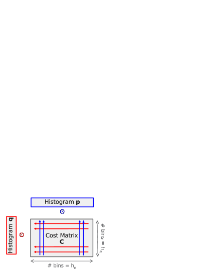
Finding an optimal solution to RWMD involves mapping the coordinates of one histogram to the closest coordinates of the other. Just like EMD, RWMD requires a cost matrix $\mathbf{C}$ that stores the pairwise distances between coordinates of $\mathbf{p}$ and $\mathbf{q}$. Finding the closest coordinates corresponds to row-wise and column-wise minimum operations in the cost matrix (see Fig. 2). To compute the first lower bound, it is sufficient to find the column-wise minimums in the cost matrix, and then perform a dot product with the weights stored in $\mathbf{p}$. Similarly, to compute the second lower bound, it is sufficient to find the row-wise minimums and then perform a dot product with the weights stored in $\mathbf{q}$. The complexity of RWMD is given by the cost of constructing the cost matrix $\mathbf{C}$: it requires quadratic time and space in the size of the input histograms. Computing the row-wise and column-wise minimums of $\mathbf{C}$ also has quadratic time complexity.

Figure 2: Quadratic-complexity RWMD computation

2.2 Linear-Complexity RWMD (LC-RWMD)

When computing RWMD between only two histograms, it is not possible to avoid a quadratic time complexity. However, in a typical information retrieval system, a query histogram is compared with a large database of histograms to identify the top-$\ell$ most similar histograms in the database. It is shown in (AtasuBigData17) that the RWMD computation involves redundant and repetitive operations in such cases, and that eliminating this redundancy reduces the average time complexity from quadratic to linear.

Assume that a query histogram is being compared with two database histograms. Assume also that the two database histograms have common coordinates. A simple replication of the RWMD computation would involve creation of two cost matrices with identical rows for the common coordinates. Afterwards, it would be necessary to perform reduction operations on these identical rows to compute the row-wise minimums. It is shown in (AtasuBigData17) that both of these redundant operations can be eliminated by 1) constructing a vocabulary that stores the union of the coordinates that occur in the database histograms, and 2) computing the minimum distances between the coordinates of the vocabulary and the coordinates of the query only once.

Table 1 lists the algorithmic parameters that influence the complexity. Table 2 shows the complexity of RWMD and LC-RWMD algorithms when comparing one query histogram with $n$ database histograms. When the number of database histograms ($n$) is in the order of the size of the vocabulary ($v$), the LC-RWMD algorithm reduces the complexity by a factor of the average histogram size ($h$). Therefore, whereas the time complexity of a brute-force RWMD implementation scales quadratically in the histogram size, the time complexity of LC-RWMD scales only linearly.

Table 1: Algorithmic Parameters

$n$	Number of database histograms
$v$	Size of the vocabulary
$m$	Dimensionality of the vectors
$h$	Average histogram size

Table 2: Complexity of Computing $n$ RWMD Distances

	Time Complexity	Space Complexity
LC-RWMD	$O(vhm+nh)$	$O(nh+vm+vh)$
RWMD	$O(nh^{2}m)$	$O(nhm)$

3 Related Work

A regularized version of the optimal transport problem can be solved more efficiently than network-flow-based approaches (Cuturi13). The solution algorithm is based on Sinkhorn’s matrix scaling technique (Sinkhorn), and thus, it is called Sinkhorn’s algorithm. Convolutional implementations can be used to reduce the time complexity of Sinkhorn’s algorithm (Solomon2015), e.g., when operating on images. Given an error term $\epsilon$, the time complexity of Sinkhorn’s algorithm is $O((h^{2}\log{h})/\epsilon^{3})$ when computing the distance between histograms of size $O(h)$ (Altschuler2017). In addition, a cost matrix has to be constructed, which incurs an additional complexity of $O(h^{2}m)$ when using $m$-dimensional coordinates.

Several other lower bounds of EMD have been proposed (assent2008efficient; xu2010efficient; ruttenberg2011indexing; wichterich2008efficient; xu2016emd; huang2016heads; huang2014melody). These lower bounds are typically used to speed-up the EMD computation based on pruning techniques. Alternatively, EMD can be computed approximately using a compressed representation (Uysal2016approximation; Pele2009).

A greedy network-flow-based approximation algorithm has also been proposed (Gottschlich2014), which does not relax the in-flow or out-flow constraints. Therefore, it is not a data-parallel algorithm and its complexity is quadratic in the histogram size. In addition, it produces an upper bound rather than a lower bound of EMD.

4 New Relaxation Algorithms

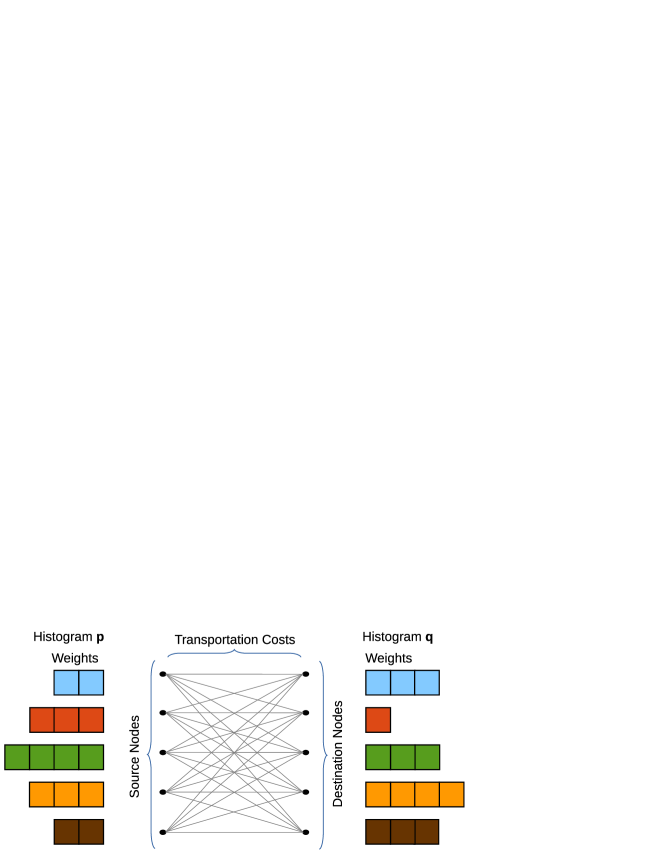
In this section, we describe improved relaxation algorithms that address the weaknesses of the RWMD measure and its linear-complexity implementation (LC-RWMD). Assume that we are measuring the distance between two histograms $\mathbf{p}$ and $\mathbf{q}$. Assume also that the coordinates of the two histograms fully overlap but the respective weights are different (see Fig. 3). In other words, for each coordinate $i$ of $\mathbf{p}$, there is an identical coordinate $j$ of $q$, for which $\mathbf{C}_{i,j}=0$. Therefore, RWMD estimates the total cost of moving $\mathbf{p}$ into $\mathbf{q}$ and vice versa as zero even though $p$ and $q$ are not the same. This condition arises, for instance, when we are dealing with dense histograms. In other cases, the data of interest might actually be sparse, but some background noise might also be present, which results in denser histograms.

Figure 3: Different histograms with identical coordinates

In general, the more overlaps there are between the coordinates of $\mathbf{p}$ and $\mathbf{q}$, the higher the approximation error of RWMD is. The main reason for the error is that when coordinate $i$ of $\mathbf{p}$ overlaps with coordinate $j$ of $\mathbf{q}$, RWMD does not take into account the fact that the respective weights $p_{i}$ and $q_{j}$ can be different. In an optimal solution, we would not be moving a mass larger than the minimum of $p_{i}$ and $q_{j}$ between these two coordinates. This is a fundamental insight that we use in the improved solutions we propose.

Given $\mathbf{p}$, $\mathbf{q}$ and $\mathbf{C}$, our goal is to define new distance measures that relax fewer EMD constraints than RWMD, and therefore, produce tighter lower bounds on EMD. Two asymmetric distances can be computed by deriving 1) the cost of moving $\mathbf{p}$ into $\mathbf{q}$ and 2) the cost of moving $\mathbf{q}$ into $\mathbf{p}$. If both are lower bounds on $\text{EMD}(\mathbf{p},\mathbf{q})$, a symmetric lower bound can be derived, e.g., by using the maximum of the two. Thus, we consider only the computation of the cost of moving $\mathbf{p}$ into $\mathbf{q}$ without loss of essential generality.

When computing the cost of moving $\mathbf{p}$ to $\mathbf{q}$ using RWMD, the in-flow constraints of (3) are removed. In other words, all the mass is transferred from $\mathbf{p}$ to the coordinates of $\mathbf{q}$, but the resulting distribution is not the same as $\mathbf{q}$. Therefore, the cost of transforming $\mathbf{p}$ to $\mathbf{q}$ is underestimated by RWMD. To achieve better approximations of $\text{EMD}(\mathbf{p},\mathbf{q})$, instead of removing the in-flow constraints completely, we propose the use of a relaxed version of these constraints:

$$F_{i,j}\leq{q}_{j}\quad\text{for all $i,j$}.$$ (4)

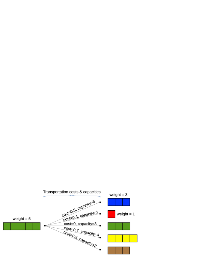
The new constraint ensures that the amount of weight that can be moved from a coordinate $i$ of $\mathbf{p}$ to a coordinate $j$ of $\mathbf{q}$ cannot exceed the weight ${q}_{j}$ at coordinate $j$. However, even if (4) is satisfied, the total weight moved to coordinate $j$ of $\mathbf{q}$ from all the coordinates of $\mathbf{p}$ can exceed ${q}_{j}$, potentially violating (3). Namely, (3) implies (4), but not vice versa.

When (4) is used in combination with (2), we have:

$$F_{i,j}\leq\min{(p_{i},q_{j})}\quad\text{for all $i,j$}.$$ (5)

Note that we are essentially imposing capacity constraints on the edges of the flow network (see Fig.4) based on (5).

Figure 4: Imposing capacity constraints on the edges

We would like to stress that in the framework of this work, which considers the discrete and not the continuous case of Wasserstein distances, the only requirement on the cost matrix is that it is nonnegative. Since any nonnegative cost $c$ between two locations can be written as the $p$-th power of the $p$-th root of $c$ for $p\geq 1$, one can assume that we are dealing with a $p$-th Wasserstein distance (Villani).

In the following subsections, we describe three new approximation methods. The Overlapping Mass Reduction (OMR) method imposes the relaxed constraint (4) only between overlapping coordinates, and is the lowest-complexity and the least accurate approximation method. The Iterative Constrained Transfers (ICT) method imposes constraint (4) between all coordinates of $\mathbf{p}$ and $\mathbf{q}$, and is the most complex and most accurate approximation method. The Approximate Iterative Constrained Transfers (ACT) method imposes constraint (4) incrementally between coordinates of $\mathbf{p}$ and $\mathbf{q}$, and is an approximation of the ICT method. Therefore, both its complexity and its accuracy are higher than those of OMR, but lower than those of ICT.

4.1 Overlapping Mass Reduction

The OMR method imposes (4) only between overlapping coordinates. The main intuition behind OMR method is that if the coordinate $i$ of $\mathbf{p}$ and the coordinate $j$ of $\mathbf{q}$ overlap (i.e., ${C}_{i,j}=0$), a transfer of $\min({p}_{i},{q}_{j})$ can take place free of cost between $\mathbf{p}$ of $\mathbf{q}$. After that, the remaining weight in $p_{i}$ is transferred simply to the second closest coordinate in $\mathbf{q}$ as this is the next least costly move. Therefore, the method computes only the top-2 smallest values in each row of $\mathbf{C}$. A detailed description is given in Algorithm 1.

OMR$\mathbf{p},\mathbf{q},\mathbf{C}$$t=0$initialize transportation cost $t$$i=1\ldots,h_{p}$iterate the indices of $\mathbf{p}$$\mathbf{s}=\text{argmin}_{2}({C}_{i,[1\ldots h_{q}]})$find top-$2$smallest ${C}_{i,\mathbf{s}[1]}==0$if the smallest value is 0 $r=\min({p}_{i},{q}_{\mathbf{s}[1]})$size of max. transfer ${p}_{i}={p}_{i}-r$move $r$units of ${p}_{i}$to ${q}_{\mathbf{s}[1]}$$t=t+{p}_{i}\cdot{C}_{i,\mathbf{s}[2]}$move the rest to ${q}_{\mathbf{s}[2]}$$t=t+{p}_{i}\cdot{C}_{i,\mathbf{s}[1]}$move all of ${p}_{i}$to ${q}_{\mathbf{s}[1]}$$t$return transportation cost $t$

Algorithm 1 Optimal Computation of OMR

4.2 Iterative Constrained Transfers

The ICT method imposes the constraint (4) between all coordinates of $\mathbf{p}$ and $\mathbf{q}$. The main intuition behind the ICT method is that because the inflow constraint (3) is relaxed, the optimal flow exiting each source node can be determined independently. For each source node, finding the optimal flow involves sorting the destination nodes in the ascending order of transportation costs, and then performing iterative mass transfers between the source node and the sorted destination nodes under the capacity constraints (4). Algorithm LABEL:alg:ict describes the ICT method in full detail.

ICT$\mathbf{p},\mathbf{q},\mathbf{C}$$t=0$initialize transportation cost $t$$i=1\ldots,h_{p}$iterate the indices of $\mathbf{p}$$\mathbf{s}=\text{argsort}({C}_{i,[1\ldots h_{q}]})$sort indices by value $l=1$initialize $l$${p}_{i}>0$while there is mass in ${p}_{i}$$r=\min({p}_{i},{q}_{\mathbf{s}[l]})$size of max. transfer ${p}_{i}={p}_{i}-r$move $r$units of ${p}_{i}$to ${q}_{\mathbf{s}[l]}$$t=t+r\cdot{C}_{i,\mathbf{s}[l]}$update cost $l=l+1$increment $l$$t$return transportation cost